Quantum Breathing of an Impurity in a One-dimensional Bath of Interacting Bosons

Abstract

By means of time-dependent density-matrix renormalization-group (TDMRG) we are able to follow the real-time dynamics of a single impurity embedded in a one-dimensional bath of interacting bosons. We focus on the impurity breathing mode, which is found to be well-described by a single oscillation frequency and a damping rate. If the impurity is very weakly coupled to the bath, a Luttinger-liquid description is valid and the impurity suffers an Abraham-Lorentz radiation-reaction friction. For a large portion of the explored parameter space, the TDMRG results fall well beyond the Luttinger-liquid paradigm.

I Introduction

The dynamics of impurities jiggling in classical and quantum liquids has tantalized many generations of physicists since the early studies on Brownian motion. In particular, the interaction of a quantum system with an external environment strongly affects its dynamics weiss ; gardiner ; caldeiraleggett . Because of this coupling, the motion of a quantum particle is characterized by a renormalized mass, decoherence, and damping. Polarons feynmann , originally studied in the context of slow-moving electrons in ionic crystals, and impurities in ³He ketterson are two prototypical examples in which the bath is bosonic and fermionic, respectively. These problems have been at the center of great interest for many decades in condensed matter physics.

Recent advances in the field of cold atomic gases reviewscoldatoms have made it possible to observe and study these phenomena from a different perspective and hence to disclose new aspects not addressed so far. It is indeed possible to accurately tune the coupling between a quantum particle and the bath and to modify the many-body nature of the bath itself. Furthermore, the dynamics of the dressed particle can be studied in real time, thus giving direct access to both mass renormalization and damping. This problem becomes of particular relevance if the bath is one-dimensional (1D). In this case interactions strongly affect the excitation spectrum of the bath giamarchi and therefore the effective dynamics of the coupled system.

The dynamics of impurities in cold atomic gases has attracted a great deal of experimental expimpurities and theoretical thimpurities attention in recent years. In particular, Catani et al. Minardi:2012 have recently studied experimentally the dynamics of K atoms (the “impurities”) coupled to a bath of Rb atoms (the “environment”) confined in 1D “atomic wires”. Motivated by Ref. Minardi:2012, we perform a time-dependent density-matrix renormalization group (TDMRG) tdmrg study of the dynamics of the breathing mode in a 1D bath of interacting bosons.

At a first sight one might think that the problem under consideration reduces to the study of a particle coupled to a Luttinger liquid LLbath . As we will discuss in the remainder of this work, it turns out that the nonequilibrium impurity dynamics eludes this type of description. This is the reason why we choose to tackle the problem with an essentially exact numerical method. Several features of the experimental data in Ref. Minardi:2012, are also seen in our simulations. As we will discuss in the conclusions, however, a detailed quantitative account of the data in Ref. Minardi:2012, may require additional ingredients and is outside the scope of the present work. Here, we highlight a number of distinct signatures of the impact of interactions on the breathing motion of an impurity, which are amenable to future experimental testing.

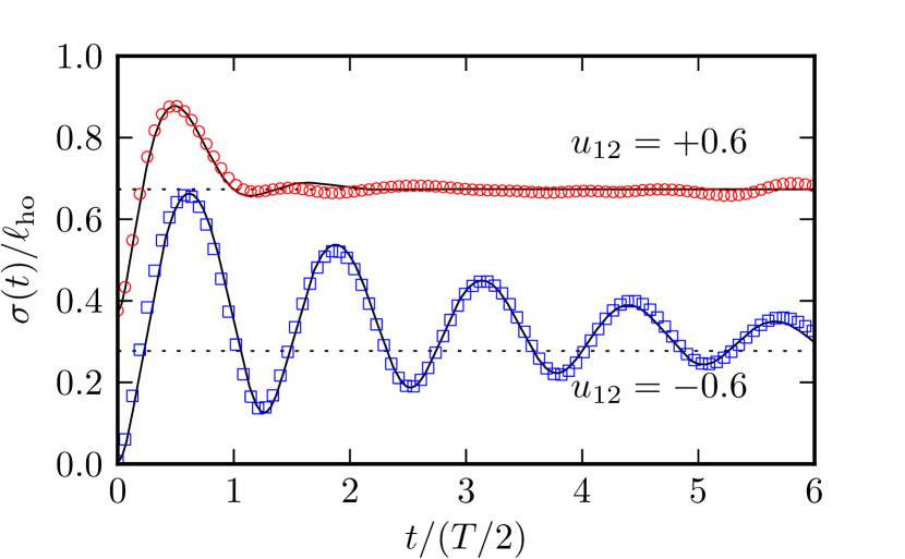
Figure 1: (Color online) The width of the impurity breathing mode $\sigma(t)$, in units of $\ell_{\rm ho}=(J_{2}/V_{2})^{1/4}\delta$ ($\delta$ is the lattice spacing), is plotted as a function of time $t$ (in units of $T/2=\pi/\omega_{2}$). Data labeled by empty symbols represent TDMRG results corresponding to two opposite values of the impurity-bath coupling constant $u_{12}$. The strength of interactions in the bath has been fixed to $u_{1}=1$. The data for $u_{12}=-0.6$ (squares) are shifted downward by $0.37~{}\ell_{\rm ho}$. The black solid lines are fits to the TDMRG data based on Eq. (3).

II Model Hamiltonian and impurity breathing mode

We consider a 1D bath of interacting bosons coupled to a single impurity confined in a harmonic potential. The bath is modeled by a Bose-Hubbard Hamiltonian with hopping $J_{1}$ and on-site repulsion $U_{1}>0$:

$${\hat{\cal H}}_{\rm B}=-J_{1}\sum_{i}({\hat{b}}^{\dagger}_{i}{\hat{b}}_{i+1}+{\rm H.c.})+U_{1}\sum_{i}{\hat{n}}^{2}_{i}+\sum_{i}W_{i}{\hat{n}}_{i}~{}.$$ (1)

Here ${\hat{b}}^{\dagger}_{i}$ (${\hat{b}}_{i}$) is a standard bosonic creation (annihilation) operator on the $i$-th site. To avoid spurious effects due to quantum confinement along the 1D system, we consider a nearly-homogeneous bath: the external confining potential $W_{i}$ is zero in a large region in the middle of the chain ($1\leq i\leq L$) and raises smoothly at the edges (see Sec. A). The local density $\langle\hat{n}_{i}\rangle=\langle\hat{b}_{i}^{\dagger}\hat{b}_{i}\rangle$ is thus essentially constant in a region of length $\sim 2L/3$. In (almost all) the results shown below we fix the number of particles in the bath to $N_{\rm bath}=22$ and distribute them over $L=250$ sites, thus keeping the average density to a small value, $\langle\hat{n}_{i}\rangle\lesssim 0.1$. For this choice of parameters the lattice is irrelevant and the model (1) is ideally suited to describe a continuum. Indeed, in the low-density limit, Eq. (1) reduces to the Lieb-Liniger model cazalilla_rmp_2011 (a mapping between the coupling constants of the two models is summarized in Sec. A). The Hamiltonian describing the impurity dynamics is

$${\hat{\cal H}}_{\rm I}(t)=-J_{2}\sum_{i}\big{(}{\hat{a}}^{\dagger}_{i}{\hat{a}}_{i+1}+{\rm H.c.}\big{)}+V_{2}(t)\sum_{i}{\bar{i}}^{2}{\hat{N}}_{i}~{},$$ (2)

with ${\hat{N}}_{i}={\hat{a}}^{\dagger}_{i}{\hat{a}}_{i}$ the impurity density operator and ${\bar{i}}=i-i_{0}$. Eq. (2) includes a kinetic term and a harmonic potential centered at $i_{0}=(L+1)/2$, whose strength $V_{2}(t)$ depends on time, mimicking the quench performed in the experimental study of Catani et al. Minardi:2012 . Because the on-site impurity density $\langle\hat{N}_{i}\rangle\lesssim 0.15$ is low, also in this case the model (2) well describes the corresponding continuum Hamiltonian (Sec. A). In this work we have fixed $J_{2}/J_{1}=2$ to take into account the mass imbalance between the impurity and bath atoms. For future purposes we introduce $\omega(t)=2\sqrt{V_{2}(t)J_{2}}/\hbar$, with $\omega_{1}=\omega(t<0)$ and $\omega_{2}=\omega(t\geq 0)$, i.e. the harmonic-potential frequencies before and after the quench, respectively. The full time-dependent Hamiltonian ${\hat{\cal H}}(t)={\hat{\cal H}}_{\rm B}+{\hat{\cal H}}_{\rm I}(t)+{\hat{\cal H}}_{\rm coupl}$ contains a further density-density coupling between bath and impurity ${\hat{\cal H}}_{\rm coupl}=U_{12}\sum_{i}{\hat{n}}_{i}{\hat{N}}_{i}$.

The quench in $\omega(t)$ excites the impurity breathing mode (BM), i.e. a mode in which the width $\sigma(t)\equiv\big{[}\sum_{i}{\bar{i}}^{2}\langle{\hat{N}}_{i}(t)\rangle\big{]}^{1/2}$, associated with the impurity density $\langle{\hat{N}}_{i}(t)\rangle$, oscillates in time footnotetime . This quantity is evaluated with the TDMRG.

III Numerical results

In Fig. 1 we illustrate the time evolution of the impurity width $\sigma(t)$ dictated by ${\hat{\cal H}}(t)$ initialcondition . Different sets of data refer to two values of the impurity-bath interaction $u_{12}=U_{12}/J_{2}$. Time $t$ is measured in units of $T/2$, where $T=2\pi/\omega_{2}$ is the period set by the harmonic-confinement frequency $\omega(t)$ after the quench. The TDMRG results (empty symbols) have been obtained by setting $u_{1}=U_{1}/J_{2}=1$ and $V_{2}(t)/J_{2}=10^{-3}$ for $t<0$ and $10^{-4}$ for $t\geq 0$ timescales .

The black solid lines are fits to the TDMRG data based on the following expression:

$$\frac{\sigma^{2}(t)}{\sigma^{2}(+\infty)}=1+\frac{e^{-2\Gamma t}}{\cos^{2}(\phi)}\sum_{i=x,p}\Delta_{i}\cos^{2}\left(t\sqrt{\Omega^{2}-\Gamma^{2}}-\theta_{i}\right)~{},$$ (3)

where $\phi=\arccos(\sqrt{1-\Gamma^{2}/\Omega^{2}})$, $\theta_{x}=\phi$, $\theta_{p}=\pi/2$, $\Delta_{x}=[\sigma(0)/\sigma(+\infty)]^{2}-1$, and $\Delta_{p}=[\sigma(+\infty)/\sigma(0)]^{2}-1$. Eq. (3) is the prediction for the BM width obtained by solving a quantum Langevin equation for the impurity position operator ${\hat{X}}(t)$ in the presence of Ohmic damping and a random Gaussian force with colored spectrum (see Sec C):

$$\partial^{2}_{t}{\hat{X}}(t)+2\Gamma\partial_{t}{\hat{X}}(t)+\Omega^{2}{\hat{X}}(t)={\hat{\xi}}(t)~{}.$$ (4)

The three parameters $\sigma(+\infty)$, $\Omega$, and $\Gamma$ (respectively the asymptotic width at long times, the frequency of the breathing oscillations, and the friction coefficient) have been used to fit the data. The initial width $\sigma(0)$ is extracted from numerical data for the ground-state width at $t<0$. Note that, in the limit in which the impurity-bath interaction is switched off ($u_{12}=0$), $\sigma(t)$ must oscillate at the frequency $2\omega_{2}$, since only even states (under exchange $x\leftrightarrow-x$) of the harmonic-oscillator potential are involved in the time evolution of a symmetric mode (like the BM). This implies $\Omega\to\omega_{2}$ in the limit $u_{12}\to 0$, where Eq. (3) reproduces the exact non-interacting dynamics.

In Fig. 2 we plot the values of the frequency $\Omega$ as a function of $u_{12}$ and for different values of $u_{1}$. Several features of the data in this figure are worth highlighting: i) the behavior of $\Omega$ is dramatically different when the sign of interactions is switched from attractive to repulsive, except at weak coupling, for a tiny region of small $u_{12}$ values; ii) the behavior becomes more symmetric with respect to the sign of $u_{12}$ as the bath is driven deeper into the Tonks-Girardeau (TG) regime, i.e., for $u_{1}\to\infty$ (in passing, we notice that our results in this limit are relevant in the context of the so-called “Fermi polaron” problem fermipolaron ); iii) the renormalization of the frequency $\Omega$ is reduced on increasing the strength of repulsive interactions in the bath $u_{1}$. It becomes almost independent of $u_{12}$ for $u_{1}\gtrsim 0.5$.

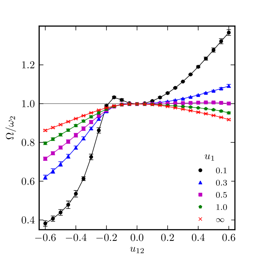
Figure 2: (Color online) The oscillation frequency of the breathing mode (in units of $\omega_{2}$) as a function of the impurity-bath Lieb-Liniger parameter $u_{12}$, for different values of the bath dimensionless coupling constant $u_{1}$. All the data in this figure have been obtained by setting $V_{2}(t)/J_{2}=10^{-3}$ for $t<0$ and $10^{-4}$ for $t\geq 0$. Error bars refer to the fitting procedure. Solid lines are guides to the eye.

Fig. 3 illustrates the dependence of the damping rate $\Gamma$ on $u_{12}$, for different values of $u_{1}$. Three features of the data are remarkable: i) $\Gamma$ displays a strong asymmetrical behavior with respect to $u_{12}=0$ away from the weak-coupling limit; ii) $\Gamma$ decreases with increasing $u_{1}$, saturating to a finite result in the TG limit; and, finally, iii) $\Gamma$ depends quadratically on $u_{12}$ for $|u_{12}|\ll 1$. The non-monotonic behavior of $\Gamma$ on the attractive side can be explained as following. For $u_{12}\approx 0$ the damping rate must be small. Increasing $|u_{12}|$ the damping rate increases because the coupling of the impurity to the bath increases. However, upon further increasing $|u_{12}|$ another effect kicks in. We have indeed discovered (data not shown here) that $\Gamma$ decreases monotonically with decreasing frequency. As shown in Fig. 2, on the attractive side $\Omega$ decreases rapidly as $|u_{12}|$ increases, thereby reducing the damping rate. The non-monotonic behavior of $\Gamma$ does not occur for $u_{12}>0$ because on the repulsive side $\Omega$ changes slightly with respect to $u_{12}$.

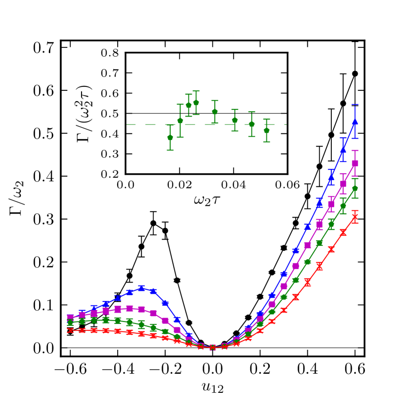
Figure 3: (Color online) Same as in Fig. 2, but for the friction coefficient $\Gamma$ (in units of $\omega_{2}$). Note that $\Gamma$ vanishes quadratically for weak impurity-bath couplings ($|u_{12}|\ll 1$) and saturates to a finite value in the limit $u_{1}\to\infty$. The inset illustrates the dependence of $\Gamma$ [in units of $\omega^{2}_{2}\tau$] on $\omega_{2}$ (in units of $1/\tau$). For each value of $\omega_{2}$, the tDMRG data (green symbols) have been obtained by performing a quench corresponding to a value of $\omega_{1}=\sqrt{10}~{}\omega_{2}$. The other parameters are: $N_{\rm bath}=40$, $L=600$ ($\langle{\hat{n}}_{i}\rangle\approx 0.07$), $u_{12}=0.1$, and $u_{1}=1$. The solid line represents the prediction $\Gamma_{\rm AL}(\omega_{2}\ll 1/\tau)/(\omega^{2}_{2}\tau)=1/2$, based on the Abraham-Lorentz model with the value of $\tau$ corresponding to $u_{1}=1$. The dashed line at $\Gamma/\omega_{2}^{2}\tau=0.44$ is the result of a best fit to the data.

The asymptotic width $\sigma(+\infty)$, shown in Fig. 4, fairly agrees with the equilibrium value at the frequency $\omega_{2}$ that one can calculate numerically. This finding seems to suggest that the impurity has nearly “thermalized” with the bath over the time scale of our simulations.

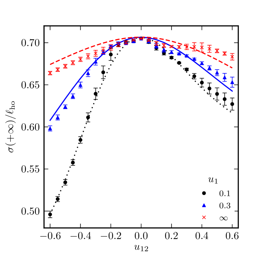
Figure 4: (Color online) Same as in Fig. 2, but for the asymptotic value $\sigma(+\infty)$ at long times of the width $\sigma(t)$ (in units of $\ell_{\rm ho}$). Here the lines are not guides to the eye, but represent the equilibrium value $\sigma_{\rm eq}$ for the width in the harmonic potential with frequency $\omega_{2}$ ($\sigma_{\rm eq}=\ell_{\rm ho}/\sqrt{2}$ for $u_{12}=0$).

IV Luttinger-liquid theory and the Abraham-Lorentz friction

We now discuss which features in Figs. 2-4 can (or cannot) be explained by employing a low-energy Luttinger-liquid description of the bath.

The Hamiltonian of a single impurity of mass $M$, described by the pair of conjugate variables (${\hat{X}},{\hat{P}}$), coupled to a bath of harmonic oscillators (the bosonic excitations of the Luttinger liquid) with dispersion $\omega_{k}=v_{\rm s}|k|$, is weiss ; Minardi:2012 :

$${\hat{\cal H}}(t)=\frac{{\hat{P}}^{2}}{2M}+V({\hat{X}},t)+\sum_{k\neq 0}\hbar\omega_{k}{\hat{\gamma}}^{\dagger}_{k}{\hat{\gamma}}_{k}+g_{12}{\hat{\rho}}({\hat{X}})~{},$$ (5)

where $V(x,t)=M\omega^{2}(t)x^{2}/2$ (the identification with the lattice model fixes $M=\hbar^{2}/(2J_{2}\delta^{2})$ with $\delta$ the lattice spacing) and $g_{12}$ is a coupling constant playing the role of $u_{12}$ in the discrete model. In Eq. (5) ${\hat{\gamma}}_{k}^{\dagger}$ (${\hat{\gamma}}_{k}$) is the creation (annihilation) operator for an acoustic-phonon mode with wave number $k$ and ${\hat{\rho}}(x)$ is the bath density operator. The sound velocity $v_{\rm s}$ is related to the Luttinger parameter $K$ of the Lieb-Liniger model by Galilean invariance haldane:1981 ; $K$ is in turn defined by the relation $\kappa=K/(\pi\hbar v_{\rm s})$, where $\kappa$ is the compressibility of the bath giamarchi . The parameters $K$ and $v_{s}$, which completely characterize the Luttinger liquid, can be expressed in terms of the coupling constants of the model in Eq. (1) (see Sec. B). We now observe that the sign of the impurity-bath coupling $g_{12}$ can be gauged away from the Hamiltonian (5) by the canonical transformation ${\hat{\gamma}}_{k}\to-{\hat{\gamma}}_{k}$. This means that if the bath was truly a Luttinger liquid, impurity-related observables such as $\Omega$ and $\Gamma$ should not depend on $g_{12}$ being attractive or repulsive. This low-energy description seems to apply only in a tiny region around $u_{12}=0$. All the deviations from this prediction seen in Figs. 2-4 have to be attributed to physics beyond the Luttinger-liquid paradigm.

The Heisenberg equation of motion induced by the Hamiltonian (5) reads (see Sec. B):

$$M\partial^{2}_{t}{\hat{X}}(t) + M\omega^{2}_{2}{\hat{X}}(t)+M\int_{0}^{t}dt^{\prime}~{}{\hat{\Gamma}}(t,t^{\prime})\partial_{t^{\prime}}{\hat{X}}(t^{\prime})$$ (6)

$$= -g_{12}\partial_{x}{\hat{\rho}(x,t)}\big{|}_{x={\hat{X}}(t)}~{},$$

where

$${\hat{\Gamma}}(t,t^{\prime})=\sum_{k\neq 0}\frac{c^{2}_{k}k^{2}}{M\omega^{2}_{k}}e^{ik{\hat{X}}(t)}e^{-ik{\hat{X}(t^{\prime})}}\cos{[\omega_{k}(t-t^{\prime})]}~{},$$ (7)

with $c_{k}=-g_{12}[Kv_{\rm s}/(\pi\hbar L)]^{1/2}|k|e^{-|k|/2k_{c}}$, is the memory kernel weiss ($k_{\rm c}$ is an ultraviolet cut-off).

If the dynamics of the impurity is slow with respect to the speed $v_{\rm s}$ of propagation of information in the bath, then “retardation effects” can be neglected and we can approximate the operator ${\hat{\Gamma}}(t,t^{\prime})$ with the following c-number $\Gamma(t-t^{\prime})=\sum_{k\neq 0}c^{2}_{k}k^{2}\cos{[\omega_{k}(t-t^{\prime})]}/(M\omega^{2}_{k})$. In this limit it is possible to show (see Sec. B) that Eq. (6) reduces to a quantum Langevin equation with an Abraham-Lorentz (AL) term, which describes the reactive effects of the emission of radiation from an oscillator jackson . This is a term of the form $-M\tau\partial_{t}^{3}{\hat{X}}(t)$ with a “characteristic time” $\tau=g_{12}^{2}K/(\pi M\hbar v_{s}^{4})$. Remarkably, neglecting the well-known “runaway” solution jackson and keeping only the damped solutions, we find that the quantum Langevin equation with the AL term yields an expression for $\sigma(t)$ after the quench which is identical to Eq. (3) with $\Gamma=\Gamma_{\rm AL}(\omega_{2})\stackrel{{\scriptstyle\omega_{2}\tau\ll 1}}{{=}}\omega^{2}_{2}\tau/2$. The full functional dependence of $\Gamma_{\rm AL}$ on $\omega_{2}$ is reported in Sec. C. Note that $\Gamma_{\rm AL}$ is proportional to $g^{2}_{12}$. This is in agreement with the TDMRG results shown in Fig. 3 in the weak-coupling $|u_{12}|\to 0$ limit. Moreover, $\Gamma_{\rm AL}$ is proportional to $K/v^{4}_{\rm s}\propto K^{5}$ (in our case $v_{\rm s}\propto K^{-1}$ from Galilean invariance haldane:1981 ) and proportional to $\omega^{2}_{2}$. The former statement implies a fast saturation of the friction coefficient to a finite value in the TG limit ($K=1$). This is in agreement with the TDMRG data shown in Fig. 3. The quadratic dependence of the damping rate on $\omega_{2}$ is also well displayed by the TDMRG data, at least for $\omega_{2}\tau\ll 1$, as shown in the inset to Fig. 3.

It is instructive to compare our findings with the experimental data of Ref. Minardi:2012, . The latter show that, in a sizable range of interaction strength $u_{12}$, the frequency of the breathing mode does not vary appreciably while the damping coefficient increases up to $\Gamma\sim 0.2~{}\omega_{2}$. As shown in Figs. 2 and 3, we do observe the same behavior for $u_{1}>0.2$. Moreover, as in the experiment, we do see that the width of the breathing mode reduces upon increasing $u_{12}$. A detailed quantitative comparison with the experiment is, however, not possible at this stage: i) one notable difference is that our calculations are carried out at $T=0$, while temperature effects seem to be important in Ref. Minardi:2012, ; ii) furthermore, the impurity trapping frequency in our calculations is considerably larger than in the experiment timescales . Extending the current calculations to take into account these differences lies beyond the scope of this work.

In summary, we have shown that, in the dynamics of an impurity coupled to a 1D bosonic bath, a Luttinger-liquid description of the bath is applicable only in a very small region of parameter space, where the impurity suffers an AL radiation-reaction friction. Among the most striking features we have found, we emphasize the non-monotonic behavior of the damping rate and the large renormalization of the oscillation frequency for attractive impurity-bath interactions.

Appendix A Lattice to continuum mapping

In our simulations we consider a 1D bath of interacting bosons coupled to a single impurity confined in a harmonic potential. The bath is modeled by a Bose-Hubbard Hamiltonian $\hat{\cal{H}}_{\rm B}$, Eq. (1) in the main text, with hopping $J_{1}$ and on-site repulsion $U_{1}>0$. The external confining potential $W_{i}$ has the following explicit form:

$$W_{i}=\begin{cases}W&i=1\,,\\ \frac{W}{2}\Big{[}1-\tanh\Big{(}\frac{3(i-(\Delta+1)/2)}{2\sqrt{(i-1)(\Delta-i)}}\Big{)}\Big{]}&1<i<\Delta\,,\\ 0&\Delta\leq i\leq L-\Delta\,,\\ \frac{W}{2}\Big{[}1+\tanh\Big{(}\frac{3(i-(2L-\Delta)/2)}{2\sqrt{(i-L+\Delta)(L-i)}}\Big{)}\Big{]}&L-\Delta<i<L\,,\\ W&i=L\,.\end{cases}$$ (8)

The parameter $\Delta$ is the length in unit of lattice sites of the left and right boundary regions, where the potential goes from 0 to a finite value $W>0$. The interpolation between the two values is as smooth as possible, since the potential, as a continuous function of $x=i\delta$ ($\delta$ being the lattice spacing), has zero derivatives of all orders at the joining points in Eq. (8). We set $\Delta=50$ lattice sites, while we used $W/J_{1}=0.1$ for $L=250$ and $N=22$ (see Fig. 5), $W/J_{1}=0.06$ for $L=600$ and $N=40$, where $L$ is the length of the (two) lattices used in our simulations, and $N$ the number of particles in the bath. In the latter case $W$ is smaller since the on-site density $n_{i}\approx 0.07$ in the middle of the chain is smaller and a weaker potential is used.

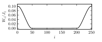
Figure 5: External confining potential for the bath in a lattice with $L=250$ sites, as defined by Eq. (8) (we set $\Delta=50$ and $W/J_{1}=0.1$).

With our choice of parameters, the local density $\langle\hat{n}_{i}\rangle=\langle\hat{b}_{i}^{\dagger}\hat{b}_{i}\rangle$ is essentially constant in a region of length $\sim 2L/3$, and kept to a low value $\langle\hat{n}_{i}\rangle\lesssim 0.1$ everywhere. At such low densities and for not too strong repulsive interaction ($U_{1}/J_{1}\lesssim 10$), the lattice is irrelevant and the model can be mapped to a Lieb-Liniger Hamiltonian cazalilla_rmp_2011 describing 1D bosons of mass $m=\hbar^{2}/(2J_{1}\delta^{2})$ interacting through a contact (repulsive) two-body potential. The upper bound for the parameter $U_{1}/J_{1}$ can be understood as follows: as the interaction between bosons is increased, the healing length of the Lieb-Liniger gas gets smaller, and, when it is comparable with $\delta$, lattice effects becomes relevant. An extensive discussion of this point can be found in Refs. Cazalilla_pra1, ; Cazalilla_pra2, ; Kollath_pra, . Other relevant parameters of the continuum model are the density $n=\langle\hat{n}_{i}\rangle/\delta$ (where $\langle\hat{n}_{i}\rangle$ is the on-site density taken in the central region where the bath is homogeneous) and the dimensionless Lieb-Liniger parameter $\gamma_{1}=mg_{1}/(\hbar^{2}n)=U_{1}/(2J_{1}\langle\hat{n}_{i}\rangle)$, where $g_{1}=U_{1}\delta>0$ is the strength of the contact repulsion between bosons.

The Hamiltonian $\hat{\cal{H}}_{\rm I}(t)$ describing the impurity is written in Eq. (2) in the main text. Given the low impurity density $\langle\hat{N}_{i}\rangle\lesssim 0.15$, also in this case the lattice model well describes the continuum Hamiltonian of a particle of mass $M=\hbar^{2}/(2J_{2}\delta^{2})$ moving in a parabolic potential $V(x,t)=V_{2}(t)(x/\delta)^{2}=M\omega^{2}(t)x^{2}/2$ (centered without loss of generality at $x=0$). The impurity mass is fixed to $M=m/2$ (thus corresponding to a ratio between the two lattice hoppings $J_{2}/J_{1}=2$), such to take into account the mass imbalance between Rb and K atoms, as experimentally done in Ref. Minardi:2012, .

The total Hamiltonian ${\hat{\cal H}}(t)={\hat{\cal H}}_{\rm B}+{\hat{\cal H}}_{\rm I}(t)+{\hat{\cal H}}_{\rm coupl}$ contains a further density-density coupling between bath and impurity, ${\hat{\cal H}}_{\rm coupl}=U_{12}\sum_{i}{\hat{n}}_{i}{\hat{N}}_{i}$, which in the continuum limit corresponds to a $\delta$-function of strength $g_{12}=U_{12}\delta$.

Appendix B Quantum Langevin equation for a particle in a Luttinger liquid

In this section we derive a quantum Langevin equation ford_pra_1988 ; weiss ; gardiner for a single particle, described by the conjugate variables $(\hat{X},\hat{P})$, that is coupled to a Luttinger liquid by a density-density interaction. The relevant Hamiltonian Minardi:2012 is given by Eq. (5) where the first two terms describe the impurity Hamiltonian, the potential $V(\hat{X})\equiv-M\omega^{2}\hat{X}^{2}/2$ representing an harmonic confining trap of frequency $\omega$ for the impurity, while the third one denotes the quadratic Luttinger Hamiltonian, in which $\hat{\gamma}_{k}^{\dagger}$ ($\hat{\gamma}_{k}$) is the creation (annihilation) operator for an acoustic-phonon mode with wave vector $k$ and dispersion $\omega_{k}=v_{\rm s}|k|$. Apart from the coupling constant $g_{12}$, the last term, which contains an ultraviolet cut-off ($k_{\rm c}$), defines the bath density operator $\hat{\rho}(\hat{X})$ of the Luttinger liquid giamarchi , and is controlled by the parameter $K$. This, in turn, controls the speed of “sound” $v_{\rm s}$ by virtue of Galilean invariance: $v_{\rm s}=\hbar\pi n/(mK)$. Repulsive interactions in the bath enter the problem through the dependence of $v_{\rm s}$ and $K$ on the Lieb-Liniger parameter $\gamma_{1}$ cazalilla_rmp_2011 .

In Eq. (5) the phonon modes couple linearly to the particle position, the latter entering through the exponential $\exp{(ik\hat{X})}$. As a consequence, the harmonic excitations of the Luttinger liquid can be integrated out leaving an effective dissipative equation (quantum Langevin equation ford_pra_1988 ) for the impurity degree of freedom. We first switch from annihilation and creation operators to (complex) position and momentum, by defining ${\hat{x}}_{k}=\sqrt{\hbar/2\omega_{k}}\big{(}{\hat{\gamma}}_{k}+{\hat{\gamma}}_{-k}^{\dagger}\big{)}$ and ${\hat{p}}_{k}=i\sqrt{\hbar\omega_{k}/2}\big{(}{\hat{\gamma}}_{k}^{\dagger}-{\hat{\gamma}}_{-k}\big{)}$, with $\big{[}\hat{x}_{k},\hat{p}_{k^{\prime}}\big{]}=i\hbar\delta_{kk^{\prime}}$. Notice that, unlike the usual position and momentum, they are complex and their adjoint are ${\hat{x}}^{\dagger}_{k}={\hat{x}}_{-k}$ and ${\hat{p}}^{\dagger}_{k}=-{\hat{p}}_{-k}$. Using these new variables one gets

$$\hat{\mathcal{H}} = \frac{\hat{P}^{2}}{2M}+V(\hat{X})+\sum_{k>0}\bigg{(}|{\hat{p}}_{k}|^{2}+\omega_{k}^{2}\Big{|}{\hat{x}}_{k}-\frac{c_{k}}{\omega_{k}^{2}}e^{-ik{\hat{X}}}\Big{|}^{2}\bigg{)}$$ (9)

$$+ \text{const.}\,,$$

where the coefficients $c_{k}=-g_{12}\sqrt{\frac{Kv_{\rm s}}{\pi\hbar L}}|k|e^{-|k|/2k_{c}}$ have been defined according to Ref. weiss, . Usually, after completing the square, some additional terms depending only on $\hat{X}$ are left out and their effect is to renormalize the potential $V(\hat{X})$. Given the peculiar non-linear nature of the coupling $\propto\exp({ik\hat{X}})$, this does not happen in our case: the terms completing the square turn out to be independent of $\hat{X}$, therefore the potential $V(\hat{X})$ is not renormalized.

The Heisenberg equations of motion dictated by Eq. (9) are given by

$$M\partial_{t}^{2}\hat{X}-F({\hat{X}}) = \sum_{k\neq 0}ikc_{k}{\hat{x}}_{k}e^{ik{\hat{X}}}\,,$$ (10)

$$\partial_{t}^{2}{\hat{x}}_{k}+\omega_{k}^{2}{\hat{x}}_{k} = c_{k}e^{-ik{\hat{X}}}\,,$$ (11)

where $F(x)\equiv-\partial_{x}V(x)$. The solution of the second equation can be immediately written down:

$${\hat{x}}_{k}(t) = {\hat{x}}_{k}(0)\cos\omega_{k}t+\frac{{\hat{p}}_{-k}(0)}{\omega_{k}}\sin\omega_{k}t$$ (12)

$$+ \frac{c_{k}}{\omega_{k}}\int_{0}^{t}dt^{\prime}\,\sin[\omega_{k}(t-t^{\prime})]\,e^{-ik{\hat{X}}(t^{\prime})}\,.$$

Integrating by parts and substituting into Eq. (10), we get

$$M\partial_{t}^{2}{\hat{X}}(t)-F({\hat{X}}(t))+M\int_{0}^{t}dt^{\prime}\,\hat{\Gamma}(t,t^{\prime})\partial_{t^{\prime}}{\hat{X}}(t^{\prime})=\sum_{k\neq 0}ikc_{k}e^{ik{\hat{X}(t)}}\Big{[}\Big{(}{\hat{x}}_{k}(0)-\frac{c_{k}}{\omega_{k}^{2}}e^{-ik{\hat{X}}(0)}\Big{)}\cos\omega_{k}t+\frac{{\hat{p}}_{-k}(0)}{\omega_{k}}\sin\omega_{k}t\Big{]}$$ (13)

with a memory kernel function

$$\hat{\Gamma}(t,t^{\prime})=\sum_{k\neq 0}\frac{c^{2}_{k}k^{2}}{M\omega_{k}^{2}}e^{ik{\hat{X}}(t)}e^{-ik{\hat{X}(t^{\prime})}}\cos\omega_{k}(t-t^{\prime})\,.$$ (14)

that depends separately on $t$ and $t^{\prime}$ (and not only on $t-t^{\prime}$), due to the presence of the two non-commuting operators ${\hat{X}}(t)$ and ${\hat{X}}(t^{\prime})$ evaluated at different times. Upon the substitution $\hat{x}_{k}(0)-c_{k}e^{-ik\hat{X}(0)}/\omega^{2}_{k}\to\hat{x}_{k}(0)$, the right hand side is just $-g_{12}\partial_{x}\hat{\rho}(x,t)|_{x=\hat{X}(t)}$. In order to see this, simply rewrite $\hat{x}_{k}(0)$ and $\hat{p}_{k}(0)$ using the corresponding annihilation and creation operators and compare to the density-density coupling in the Hamiltonian (5). As discussed in Ref. weiss, , one can forget about the term $\propto e^{ik\hat{X}(0)}$ in the right hand side of Eq. (13), since it has no effect when taking averages on the equilibrium state of the bath coupled to the particle at $t=0$ (as a consequence the stochastic term in the quantum Langevin equation (13) has zero average: $\langle\partial_{x}\hat{\rho}(\hat{X}(t),t)\rangle=0$).

When evaluating the noise correlator one runs into difficulties since $e^{ik\hat{X}(t)}e^{-ik\hat{X}(t^{\prime})}\neq e^{ik[\hat{X}(t)-\hat{X}(t^{\prime})]}$. In the limit when the particle has a small velocity with respect to $v_{\rm s}$, we can however perform the following approximation:

$$e^{ik\hat{X}(t)}e^{-ik\hat{X}(t^{\prime})}e^{\pm iv_{\rm s}|k|(t-t^{\prime})}\approx e^{\pm iv_{\rm s}|k|(t-t^{\prime})}\,,$$ (15)

since in this case the product of the first two exponentials is assumed to be slowly varying with respect to the third one. Therefore in this limit the noise correlator $\hat{\Xi}(t,t^{\prime})\equiv g_{12}^{2}\langle[\partial_{x}\hat{\rho}({\hat{X}}(t),t)]^{\dagger}\partial_{x}\hat{\rho}({\hat{X}}(t^{\prime}),t^{\prime})\rangle$ reads:

$$\begin{split}\hat{\Xi}(t,t^{\prime})\approx\frac{g_{12}^{2}K}{\pi\hbar v_{s}^{4}}\int_{0}^{+\infty}\frac{d\omega}{2\pi}e^{-\omega/\omega_{c}}\hbar\omega^{3}\,\times\\ \times\left(\coth\frac{\beta\hbar\omega}{2}\cos\omega(t-t^{\prime})-i\sin\omega(t-t^{\prime})\right)\,,\end{split}$$ (16)

where we passed in the continuum by substituting the series over $k$ with an integral over the frequencies $\omega$. In the same approximation, the memory kernel (14) entering the third term in the left hand side of Eq. (13) reads

$$\hat{\Gamma}(t,t^{\prime})\approx\frac{2g_{12}^{2}K}{\pi\hbar v_{\rm s}^{4}}\int_{0}^{+\infty}\frac{d\omega}{2\pi}e^{-\omega/\omega_{c}}\omega^{2}\cos\omega(t-t^{\prime})\,.$$ (17)

Notice that, when the cut-off $\omega_{c}$ goes to infinity, this kernel basically reduces to the second derivative of a delta function:

$$\hat{\Gamma}(t,t^{\prime})\stackrel{{\scriptstyle\omega_{c}\to+\infty}}{{=}}-M\tau\delta^{\prime\prime}(t-t^{\prime})\,,$$ (18)

where $\tau=g_{12}^{2}K/(\pi M\hbar v_{\rm s}^{4})$ is the proper time scale.

The relation $\Re\big{[}\widetilde{\Xi}(\omega)\big{]}=M\hbar\omega\coth(\beta\hbar\omega/2)\Re\big{[}\widetilde{\Gamma}(\omega)\big{]}$ states the fluctuation-dissipation theorem ford_pra_1988 ; weiss ; gardiner , and holds between the real parts of the Fourier transforms of the noise correlator, $\widetilde{\Xi}(\omega)$, and of the memory kernel, $\widetilde{\Gamma}(\omega)$. This ensures the consistency of the slow-particle approximation, see Eq. (15). Within this approximation, the quantum Langevin equation takes the linear form

$$M\partial_{t}^{2}{\hat{X}}(t)-F({\hat{X}}(t))-M\tau\partial_{t}^{3}{\hat{X}}(t)=-g_{12}\partial_{x}\hat{\rho}(\hat{X}(t),t)\,.$$ (19)

The fact that the position operator appears on the right hand side as an argument of the bath density does not spoil linearity, since the noise correlator is independent of the difference $X(t)-X(t^{\prime})$ in the slow-particle approximation.

Considering $\hat{X}(t)$ as a classical variable, the $k$-sum in the third term on the left of Eq. (13) can be easily performed, thus obtaining the following classical Langevin equation:

$$\begin{split}&M\partial_{t}^{2}X(t)-F({X}(t))-\frac{g_{12}^{2}K}{2\pi\hbar v^{3}_{\rm s}}\int_{0}^{t}dt^{\prime}\,\partial_{t}^{3}{X}(t^{\prime})\,\times\\ &\times\sum_{\epsilon=\pm}\big{[}\delta\big{(}{X}(t)-{X(t^{\prime})}+\epsilon\,v_{\rm s}(t-t^{\prime})\big{)}\big{]}=-g_{12}\partial_{x}{\rho}({X}(t),t)\,.\end{split}$$ (20)

From here it is apparent that the particle is interacting at point $X(t)$ and time $t$ with the phonons (density fluctuations in the Luttinger liquid) emitted by itself at point $X(t^{\prime})$ in a past time $t^{\prime}$. This is similar to radiation damping of the motion of a charge particle, where the role of the electromagnetic field is now played by the Luttinger liquid. The problem of damping due to the emission of radiation is a very old one and the classical version of Eq. (19) has been known in this context for a long time as the Abraham-Lorentz equation jackson .

The quantum version of Eq. (LABEL:eq:rad_damping) is more complicated, due to its operatorial character (in this case indeed $e^{ik\hat{X}(t)}e^{-ik\hat{X}(t^{\prime})}\neq e^{ik[\hat{X}(t)-\hat{X}(t^{\prime})]}$). In the specific, Eq. (19) has been obtained under the assumption (15), thus it is expected to be valid only when the particle does not move too fast with respect to the phonons. This can be quantified by considering a small value for the ratio $\nu$ between the maximum velocity of the impurity distribution when it expands, $\omega_{2}\ell_{\rm ho}^{2}/\sigma(0)$ (here $\ell_{\rm ho}=\sqrt{\hbar/M\omega_{2}}$ is the harmonic oscillator length), and the velocity of sound $v_{s}$. Such ratio is independent of the trap frequency, and is fixed only by the initial squeezing through the uncertainty principle – if the uncertainty in position is $\sigma(0)$ then the uncertainty in velocity is $\hbar/(M\sigma(0))$.

In our simulations this parameter is actually not so small. An estimate can be given as follows: the velocity of sound $v_{\rm s}$ is a fraction of the Fermi velocity for a gas of free fermions at the same density, say $v_{\rm s}\sim\hbar\pi n/m$, the initial squeezing is $\sigma(0)/\ell_{\rm ho}\approx 0.4$ and the density $n\ell_{\rm ho}\approx 1$, so

$$\nu=\frac{\omega_{2}\ell_{\rm ho}^{2}}{v_{s}\sigma(0)}=\frac{\hbar}{Mv_{\rm s}\sigma(0)}=\frac{m/M}{\pi\sigma(0)n}\approx 1.6\,.$$ (21)

So we expect corrections to Eq. (19) due to retardation effects embodied in Eq. (13).

Appendix C Impurity breathing mode within the quantum Langevin equation

In this section we derive the function used to fit the TDMRG data [see Eq. (3) in the main text]. We show how it can be obtained starting both from the quantum Langevin equation for an ohmic bath weiss ; gardiner :

$$M\partial^{2}_{t}{\hat{X}}(t)+2M\Gamma\partial_{t}{\hat{X}}(t)+M\omega^{2}_{2}{\hat{X}}(t)={\hat{\xi}}(t)\,,$$ (22)

with noise correlator

$$\Xi(t) = \langle{\hat{\xi}}(t){\hat{\xi}}(0)\rangle$$

$$= \frac{2M\Gamma}{\pi}\int_{0}^{+\infty}d\omega\hbar\omega\left[\coth\frac{\beta\hbar\omega}{2}\cos\omega t-i\sin\omega t\right]\,,$$

and from the Langevin equation (19) in the previous section, with a noise correlator given by Eq. (16) that describes a superohmic bath weiss ; gardiner .

The predictions for the oscillation frequency and the damping coefficient are different in the two cases. However it is possible to treat both equations in the same way, because their respective Green functions $G(\omega)$ have a similar pole structure in the frequency domain. Both have two poles at complex frequencies $\omega_{\pm}$ with negative imaginary part ($\Gamma>0$):

$$\omega_{\pm}=\pm\sqrt{\Omega^{2}-\Gamma^{2}}-i\Gamma\,.$$ (24)

These are the physically relevant ones and correspond to exponentially decaying solutions. It is essential for our purposes that $\omega_{+}=-\omega_{-}^{*}$. We point out that Eq. (19) is of third order and its Green function has a third pole in the upper half of the complex plane that corresponds to an unphysical diverging solution, also called “run-away” solution jackson , which will be discarded in the following. Note that, while for the ohmic case $\Omega$ is equal to the trap frequency $\omega_{2}$, and $\Gamma$ is exactly the coefficient that appears in Eq. (22), for the Langevin equation in (19) one has a more complex dependence on the trap frequency $\omega_{2}$ and on the time scale $\tau$. In the specific, the three roots of the cubic characteristic equation $-i\omega^{3}\tau-\omega^{2}+\omega_{2}^{2}=0$ read

$$\omega_{\pm}=\pm\frac{1}{2\sqrt{3}\tau}\left(z-z^{-1}\right)+\frac{i}{3\tau}\left(1-\frac{z+z^{-1}}{2}\right)\,,$$ (25)

$$\omega_{\rm run-away}=\frac{i}{3\tau}\left[1+z+z^{-1}\right]\,,$$ (26)

with

$$z^{\pm 1}=\bigg{(}\frac{27\omega_{2}^{2}\tau^{2}+2\pm\sqrt{(27\omega_{2}^{2}\tau^{2}+2)^{2}-4}}{2}\bigg{)}^{1/3}\,.$$ (27)

Note that $\omega_{\pm}$ have always negative imaginary part, while $\omega_{\rm run-away}$ has positive imaginary part and zero real part.

The symmetry of the physical roots allows us to write the solution of both the two Langevin equations as

$$\begin{split}\hat{X}(t)&=\hat{X}(0)e^{-\Gamma t}\cos\sqrt{\Omega^{2}-\Gamma^{2}}t\\ &\quad+\frac{\partial_{t}\hat{X}(0)+\Gamma\hat{X}(0)}{\sqrt{\Omega^{2}-\Gamma^{2}}}e^{-\Gamma t}\sin\sqrt{\Omega^{2}-\Gamma^{2}}t\\ &\quad+\int_{0}^{t}dt^{\prime}G(t-t^{\prime})\hat{\xi}(t^{\prime})\,,\end{split}$$ (28)

$\hat{\xi}(t)$ and $G(t)$ denoting the noise term and the Green function respectively.

Using Eq. (28), and the fact that $\langle\hat{\xi}(t)\rangle=0$, we can evaluate some asymptotic averages which turn out to be useful to calculate the impurity breathing mode. Some of them are null:

$$\langle\hat{X}(+\infty)\rangle=\langle\partial_{t}\hat{X}(+\infty)\rangle=\langle\{\hat{X},\partial_{t}\hat{X}\}\rangle_{t\to+\infty}=0\,,$$ (29)

while other ones, such as $\langle\hat{X}^{2}(+\infty)\rangle$ and $\langle(\partial_{t}\hat{X}(+\infty))^{2}\rangle$, can be implicitly written in terms of the spectral function weiss , whose form depends on the nature of the bath. Finally, call $\hat{E}(t)=\int_{0}^{t}dt^{\prime}G(t-t^{\prime})\hat{\xi}(t^{\prime})$ and note that

$$\langle\hat{X}(0)\hat{E}(t)\rangle=\langle\partial_{t}\hat{X}(0)\hat{E}(t)\rangle=0\,.$$ (30)

With all these results at hand, the average of $\hat{X}^{2}(t)$ can be calculated at an arbitrary time $t$. Suppose that the particle starts its motion at $t=-\infty$ in a squeezed harmonic potential. At $t=0$ it will have equilibrated with the bath, and expectation values are taken on the equilibrium state of the whole system, with the particle at rest in the squeezed harmonic potential. Then the frequency of the harmonic confinement is suddenly quenched to a new value $\omega_{2}$. The width of the impurity density distribution as a function of time, for $t>0$, can be explicitly calculated by taking the square of Eq. (28) on the global state: $\sigma^{2}(t)=\langle\hat{X}^{2}(t)\rangle$. Using Eqs. (29)-(30), one ends up with the following expression:

$$\sigma^{2}(t)=\langle\hat{E}^{2}(t)\rangle+\frac{e^{-2\Gamma t}}{\cos^{2}\phi}\bigg{[}\langle\hat{X}^{2}(0)\rangle\cos^{2}\big{(}\sqrt{\Omega^{2}-\Gamma^{2}}t-\phi\big{)}\\ +\frac{\langle(\partial_{t}\hat{X}(0))^{2}\rangle}{\Omega^{2}}\sin^{2}\sqrt{\Omega^{2}-\Gamma^{2}}t\bigg{]}\,,$$ (31)

with $\phi=\arcsin(\Gamma/\Omega)$. It is not necessary to calculate explicitly the average $\langle\hat{E}^{2}(t)\rangle$, since it has to cancel exactly the other terms in Eq. (31) when $\langle\hat{X}^{2}(0)\rangle=\langle\hat{X}^{2}(+\infty)\rangle$ and $\langle(\partial_{t}\hat{X}(0))^{2}\rangle=\langle(\partial_{t}\hat{X}(+\infty))^{2}\rangle$. Therefore the final result is

$$\sigma^{2}(t)=\sigma^{2}(+\infty)\bigg{\{}1+\frac{e^{-2\Gamma t}}{\cos^{2}\phi}\Big{[}\Delta_{x}\cos^{2}\big{(}\sqrt{\Omega^{2}-\Gamma^{2}}t-\phi\big{)}\\ +\Delta_{p}\sin^{2}\sqrt{\Omega^{2}-\Gamma^{2}}t\Big{]}\bigg{\}}\,,$$ (32)

where the definitions below have been used:

$$\Delta_{x}=\frac{\langle\hat{X}^{2}(0)\rangle-\langle\hat{X}^{2}(+\infty)\rangle}{\langle\hat{X}^{2}(+\infty)\rangle},$$ (33)

$$\Delta_{p}=\frac{\langle(\partial_{t}\hat{X}(0))^{2}\rangle-\langle(\partial_{t}\hat{X}(+\infty))^{2}\rangle}{\Omega^{2}\langle\hat{X}^{2}(+\infty)\rangle}\,.$$ (34)

We employ Eq. (32) in our fitting procedure as follows. $\Delta_{x}$ and $\Delta_{p}$ are fixed to their non-interacting values

$$\Delta_{x}=\frac{\sigma^{2}(0)}{\sigma^{2}(+\infty)}-1\,\quad\text{and}\quad\Delta_{p}=\frac{\sigma^{2}(+\infty)}{\sigma^{2}(0)}-1\,,$$ (35)

while $\sigma(+\infty)$, $\Omega$, $\Gamma$ are used as fitting parameters. The initial width $\sigma(0)$ is provided directly by the numerical data. This choice allows reliable fits that smoothly interpolate with the exact non-interacting result:

$$\sigma(t)=\sqrt{\sigma^{2}(0)\cos^{2}\omega_{2}t+\frac{\ell_{\rm ho}^{4}}{4\sigma^{2}(0)}\sin^{2}\omega_{2}t}\,.$$ (36)

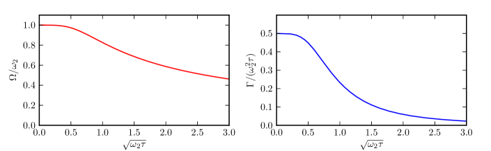
Figure 6: (Color online) Plot of $\Omega/\omega_{2}$ and $\Gamma/\omega_{2}$ as a function of $\sqrt{\omega_{2}\tau}\propto g_{12}$, to allow a comparison with the results in the main text. In particular, after expanding Eq. (25) for $\omega_{2}\tau\ll 1$, we get: $\Omega/\omega_{2}\approx 1-\omega_{2}^{2}\tau^{2}/2$ and $\Gamma/(\omega_{2}^{2}\tau)\approx 1/2$.

Surprisingly, the same functional form of Eq. (32) holds for two quite different models. This is due to the form of the two relevant complex frequencies [see Eq. (24)] that applies to both of them. However the two models provide distinct predictions for the modulus $\Omega=|\omega_{\pm}|$ and the damping coefficient $\Gamma$, with some appreciable differences. For an ohmic bath one has $\Omega=\omega_{2}$, so that the frequency is not renormalized in this case. Moreover $\Gamma$ is a fixed time constant independent of the trap frequency. For the superohmic case of Eq. (19), for $\omega_{2}\tau\ll 1$ it can be shown that $\Omega/\omega_{2}$ is a function of $\omega_{2}\tau$, the same holds for $\Gamma/\omega_{2}$ (see Fig. 6). Notice also that $\omega_{\pm}$ always has a non-zero real part, therefore there is no overdamped solution for any value of $\tau$.

Finally we emphasize that the functional form given in Eq. (32) is essential to extract the parameters $\Omega$, $\Gamma$ and $\sigma(+\infty)$ from the numerical data. Indeed we have verified that the numerical fits performed using the functional form Minardi:2012

$$\sigma(t)=\sigma(+\infty)+Ae^{-\Gamma t}\cos(\sqrt{\Omega^{2}-\Gamma^{2}}t-\phi)\,,$$ (37)

with $A$ being the oscillation amplitude (grey lines in Fig. 7), are significantly different from the ones that are obtained employing Eq. (32) (black lines in Fig. 7). For example, the fit done with Eq. (37) often overestimates the asymptotic with $\sigma(+\infty)$.

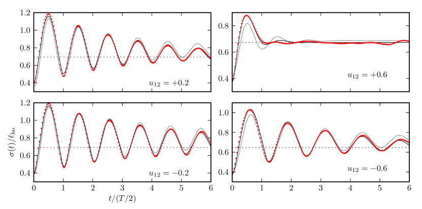
Figure 7: (Color online) Width of the impurity breathing mode $\sigma(t)$ (in units of $\ell_{\rm ho}=[\hbar/(M\omega_{2})]^{1/2}$) as a function of time $t$ (in units of $T/2=\pi/\omega_{2}$). Data in different panels corresponds to four values of the impurity-bath Lieb-Liniger parameter $u_{12}$, for a fixed value of the bath Lieb-Liniger parameter $u_{1}=1$. Filled red circles label the tDMRG results. The black solid lines are fits to the tDMRG data using Eq. (32). The thin grey lines are obtained by employing the fitting function in Eq. (37).

- (1) U. Weiss, Quantum Dissipative Systems (World Scientific, Singapore, 2008).
- (2) C.W. Gardiner and P. Zoller, Quantum Noise (Springer, Berlin, 2004).
- (3) A.O. Caldeira and A.J. Leggett, Physica A 121, 587 (1983); A.J. Leggett, S. Chakravarty, A.T. Dorsey, M.P.A. Fisher, A. Garg, and W. Zwerger, Rev. Mod. Phys. 59, 1 (1987).
- (4) R.P. Feynman, Statistical Mechanics: A Set of Lectures, (Addison Wesley, Reading MA, 1972).
- (5) The Physics of Liquid and Solid Helium, edited by K.H. Benneman and J.B. Ketterson (Wiley, New York, 1978).
- (6) I. Bloch, J. Dalibard, and W. Zwerger, Rev. Mod. Phys. 80, 885 (2008).
- (7) T. Giamarchi, Quantum Physics in One Dimension (Oxford University Press, Oxford, 2004).
- (8) J. Catani, L. De Sarlo, G. Barontini, F. Minardi, and M. Inguscio, Phys. Rev. A77, 011603 (2008); S. Palzer, C. Zipkes, C. Sias, and M. Köhl, Phys. Rev. Lett. 103, 150601 (2009); B. Gadway, D. Pertot, R. Reimann, and D. Schneble, ibid. 105, 045303 (2010); S. Schmid, A. Härter, and J.H. Denschlag, ibid. 105, 133202 (2010); C. Zipkes, S. Palzer, C. Sias, and M. Köhl, Nature 464, 388 (2010).
- (9) F.M. Cucchietti and E. Timmermans, Phys. Rev. Lett. 96, 210401 (2006); K. Sacha and E. Timmermans, Phys. Rev. A73, 063604 (2006); M. Bruderer, A. Klein, S.R. Clark, and D. Jaksch, ibid 76, 011605 (2007); M. Bruderer, A. Klein, S.R. Clark, and D. Jaksch, New J. Phys. 10, 033015 (2008); J. Tempere, W. Casteels, M.K. Oberthaler, S. Knoop, E. Timmermans, and J.T. Devreese, Phys. Rev. B80, 184504 (2009); A. Privitera and W. Hofstetter, Phys. Rev. A82, 063614 (2010); D.H. Santamore and E. Timmermans, New J. Phys. 13, 103029 (2011); W. Casteels, T. Van Cauteren, J. Tempere, and J.T. Devreese, Laser Phys. 21, 1480 (2011); W. Casteels, J. Tempere, and J.T. Devreese, Phys. Rev. A83, 033631 (2011) and 84, 063612 (2011); W. Casteels, J. Tempere, and J.T. Devreese, J. Low Temp. Phys. 162, 266 (2011); T.H. Johnson, S.R. Clark, M. Bruderer, and D. Jaksch, Phys. Rev. A84, 023617 (2011).
- (10) J. Catani, G. Lamporesi, D. Naik, M. Gring, M. Inguscio, F. Minardi, A. Kantian, and T. Giamarchi, Phys. Rev. A85, 023623 (2012).
- (11) See e.g. U. Schollwöck, Ann. Phys. (NY) 326, 96 (2011).
- (12) See, for example, A.H. Castro Neto and A.O. Caldeira, Phys. Rev. B46, 8858 (1992); ibid. 50, 4863 (1994); ibid. 52, 4198 (1995); A.H. Castro Neto and M.P.A. Fisher, ibid. 53, 9713 (1996); J. Bonart and L.F. Cugliandolo, arXiv:1203.5273.
- (13) M.A. Cazalilla, R. Citro, T. Giamarchi, E. Orignac, and M. Rigol, Rev. Mod. Phys. 83, 1405 (2011).
- (14) Here is a shorthand for , being the state of the system at time .
- (15) The initial condition is given by the ground state of at times .
- (16) This implies an oscillation period , to be compared with in Ref. Minardi:2012, .
- (17) See, for example, A. Schirotzek, C.-H. Wu, A. Sommer, and M.W. Zwierlein, Phys. Rev. Lett. 102, 230402 (2009); A. Sommer, M. Ku, and M.W. Zwierlein, New J. Phys. 13, 055009 (2011); C. Kohstall, M. Zaccanti, M. Jag, A. Trenkwalder, P. Massignan, G.M. Bruun, F. Schreck, and R. Grimm, arXiv:1112.0020 – Nature (2012), published online; M. Koschorreck, D. Pertot, E. Vogt, B. Fröhlich, M. Feld, and M. Köhl, arXiv:1203.1009 – Nature (2012), published online.
- (18) F.D.M. Haldane, Phys. Rev. Lett. 47, 1840 (1981).
- (19) J.D. Jackson, Classical Electrodynamics (Wiley, New York, 1998).
- (20) M.A. Cazalilla, Phys. Rev. A67, 053606 (2003).
- (21) M.A. Cazalilla, Phys. Rev. A70, 041604(R) (2004).
- (22) C. Kollath, U. Schollwöck, J. von Delft, W. Zwerger, Phys. Rev. A71, 053606 (2005).
- (23) G.W. Ford, J.T. Lewis, and R.F. O’Connell, Phys. Rev. A37, 4419 (1988).