GRMHD simulations of accretion onto Sgr A*: How important are radiative losses?

Abstract

We present general relativistic magnetohydrodynamic (GRMHD) numerical simulations of the accretion flow around the supermassive black hole in the Galactic centre, Sagittarius A* (Sgr A*). The simulations include for the first time radiative cooling processes (synchrotron, bremsstrahlung, and inverse Compton) self-consistently in the dynamics, allowing us to test the common simplification of ignoring all cooling losses in the modeling of Sgr A*. We confirm that for Sgr A*, neglecting the cooling losses is a reasonable approximation if the Galactic centre is accreting below $\sim 10^{-8}M_{\odot}~{}{\rm yr^{-1}}$ i.e. $\dot{M}<10^{-7}\dot{M}_{Edd}$. But above this limit, we show that radiative losses should be taken into account as significant differences appear in the dynamics and the resulting spectra when comparing simulations with and without cooling. This limit implies that most nearby low-luminosity active galactic nuclei are in the regime where cooling should be taken into account.

We further make a parameter study of axisymmetric gas accretion around the supermassive black hole at the Galactic centre. This approach allows us to investigate the physics of gas accretion in general, while confronting our results with the well studied and observed source, Sgr A*, as a test case. We confirm that the nature of the accretion flow and outflow is strongly dependent on the initial geometry of the magnetic field. For example, we find it difficult, even with very high spins, to generate powerful outflows from discs threaded with multiple, separate poloidal field loops.

1 Introduction

Super-massive black holes (SMBHs) of millions to billions of solar masses are believed to exist in the centre of most galaxies. The Galactic center black hole candidate, Sgr A*, is the closest and best studied SMBH, making it the perfect source to test our understanding of galactic nuclei systems in general. This compact object was first observed as a radio source by Balick & Brown (1974). Since then, observations have constrained important parameters of Sgr A*, such as its mass and distance, estimated at $M=4.3\pm 0.5\times 10^{6}M_{\odot}$ and $D=8.3\pm 0.35~{}{\rm kpc}$, respectively (Reid, 1993; Schödel et al., 2002; Ghez et al., 2008; Gillessen et al., 2009). The accretion rate has also been constrained by polarisation measurements, using Faraday rotation arguments (Aitken et al., 2000; Bower et al., 2003; Marrone et al., 2007) and is estimated to be in the range $2\times 10^{-9}<\dot{M}<2\times 10^{-7}M_{\odot}~{}{\rm yr^{-1}}$. Other key parameters, such as the spin, inclination, and magnetic field configuration, are still under investigation.

Multi-wavelength observations of Sgr A* have been performed from the radio to the gamma ray (see reviews by Melia & Falcke 2001; Genzel et al. 2010, and references therein). More recently, important progress has been achieved in the infrared (IR; e.g., Schoedel et al., 2011) and sub-millimeter (sub-mm) domains. All observations agree that Sgr A* is a very under-luminous and weakly accreting black hole; indeed its accretion rate is lower than has been observed in any other accreting system.

In the near future, the next milestone will be observing the first black hole shadow from Sgr A* (Falcke et al., 2000; Dexter et al., 2010) with the proposed “Event Horizon Telescope” (Doeleman et al., 2008, 2009; Fish et al., 2011) thanks to the capabilities of very long base interferometry at sub-mm wavelengths. Such a detection would be the first direct evidence for a black hole event horizon, and may also constrain the spin of Sgr A*. In order to make accurate predictions for testing with the Event Horizon Telescope, however, we need to have reliable models for the plasma conditions and geometry in the accretion (in/out)flow. General relativistic magnetohydrodynamic (MHD) simulations offer significant promise for this class of study, as they can provide both geometrical and spectral predictions.

Sgr A* has already been modeled in several numerical studies (e.g., Goldston et al., 2005; Mościbrodzka et al., 2009; Dexter et al., 2009; Dexter et al., 2010; Hilburn et al., 2010; Shcherbakov et al., 2010; Shiokawa et al., 2012; dolence12; Dexter & Fragile, 2012). All of these models consist of two separate codes: a GRMHD code describing the dynamics, and then a subsequent code to calculate the radiative emission based on the output of the first one. The under-luminous and under-accreting state of Sgr A* ($L_{\rm bol}\simeq 10^{-9}L_{\rm Edd}$ and $L_{\rm X-Ray}\simeq 10^{33}$ erg/s in the 0.5 to 10 keV band, where $L_{\rm Edd}$ is the Eddington luminosity; Baganoff et al. 2003), is the common argument given to justify ignoring the cooling losses and simplify the description of Sgr A*. Even though this approach seems reasonable, especially for the peculiar case of Sgr A*, we propose to quantify to what extent it really applies. This question is especially important if one wants to extend these studies to more typical nearby low-luminosity active galactic nuclei (LLAGN). An important example is the nuclear black hole in M87, which is the other major target for mm-VLBI and is significantly more luminous than Sgr A* ($L/L_{\rm Edd}\sim 10^{-6}-10^{-4}$).

To test whether or not ignoring the radiative cooling losses is a reasonable approximation, we need to take into account the radiative losses self-consistently in the dynamics, which is now possible with the Cosmos++ astrophysical fluid dynamics code (Anninos et al., 2005; Fragile & Meier, 2009). By allowing the gas to cool, energy can be liberated from the accretion flow, potentially changing the dynamics of the system. The basic result that we show in this paper is that cooling is indeed negligible at the lowest end of the possible accretion rate range of Sgr A*, but plays an increasingly important role in the dynamics and the resulting spectra for higher accretion rates (relevant for most nearby LLAGN and even at the high end of the range of Sgr A*).

This paper is organized as follows: In Section 2 we describe the new version of Cosmos++ used to perform this study. In Section 3 we present the initial set-up of the simulations. In Section 4 we show the importance of the accretion rate parameter and assess the effect of including radiative cooling. In Section 5 we perform a parameter survey to investigate the influence of the initial magnetic field configuration and the spin of the SMBH (we also discuss the effect of a retrograde spin on the dynamics) on the resulting accretion disc structure and outflow. In Section 6 we end with our conclusions and outlook. The spectra generated from these simulations are analyzed in detail in a companion paper (Drappeau et al., in preparation, hereafter referred to in the text as D12).

2 Numerical Method

2.1 GRMHD Equations

Within Cosmos++ we solve the following set of conservative, general relativistic MHD equations, including radiative cooling,

$$\partial_{t}D+\partial_{i}(DV^{i}) = 0~{},$$ (1)

$$\partial_{t}{\cal E}+\partial_{i}(-\sqrt{-g}~{}T^{i}_{0}) = -\sqrt{-g}~{}T^{\kappa}_{\lambda}~{}\Gamma^{\lambda}_{0\kappa}+\sqrt{-g}~{}\Lambda u_{0}~{},$$ (2)

$$\partial_{t}{\cal S}_{j}+\partial_{i}(\sqrt{-g}~{}T^{i}_{j}) = \sqrt{-g}~{}T^{\kappa}_{\lambda}~{}\Gamma^{\lambda}_{j\kappa}-\sqrt{-g}~{}\Lambda u_{j}~{},$$ (3)

$$\partial_{t}\mathcal{B}^{j}+\partial_{i}(\mathcal{B}^{j}V^{i}-\mathcal{B}^{i}V^{j}) = 0~{},$$ (4)

where $D=W\rho$ is the generalized fluid density, $W=\sqrt{-g}u^{0}$ is the generalized boost factor, $V^{i}=u^{i}/u^{0}$ is the transport velocity, $u^{\mu}=g^{\mu\nu}u_{\nu}$ is the fluid 4-velocity, $g_{\mu\nu}$ is the 4-metric, $g$ is the 4-metric determinant,

$${\cal E} = -\sqrt{-g}T^{0}_{0}$$ (5)

$$= -Wu_{0}\left(\rho h+2P_{B}\right)-\sqrt{-g}\left(P+P_{B}\right)+\sqrt{-g}b^{0}b_{0}$$

is the total energy density, $h=1+\epsilon+P/\rho$ is the specific enthalpy, $\epsilon$ is the specific internal energy, $P$ is the fluid pressure, $P_{B}$ is the magnetic pressure, $T^{\kappa}_{\lambda}$ is the stress-energy tensor, $\Lambda$ is the cooling function, and

$${\cal S}_{\mu}=\sqrt{-g}T^{0}_{j}=Wu_{j}\left(\rho h+2P_{B}\right)-\sqrt{-g}b^{0}b_{j}$$ (6)

is the covariant momentum density. With indices, $\Gamma$ indicates the geometric connection coefficients of the metric. Without indices, $\Gamma$ is the adiabatic index. For this work we use an ideal gas equation of state (EOS),

$$P=(\Gamma-1)\rho\epsilon~{},$$ (7)

with $\Gamma=5/3$.

There are multiple representations of the magnetic field in our equations: $b^{\mu}$ is the magnetic field measured by an observer comoving with the fluid, which can be defined in terms of the dual of the Faraday tensor $b^{\mu}\equiv u_{\nu}{{}^{*}F^{\mu\nu}}$, and $\mathcal{B}^{j}=\sqrt{-g}B^{j}$ is the boosted magnetic field 3-vector. The un-boosted magnetic field 3-vector $B^{i}={{}^{*}F^{\mu i}}$ is related to the comoving field by

$$B^{i}=u^{0}b^{i}-u^{i}b^{0}~{}.$$ (8)

The magnetic pressure is $P_{B}=b^{2}/2=b^{\mu}b_{\mu}/2$. Note that, unlike in previous versions of Cosmos++, we have absorbed the factor of $\sqrt{4\pi}$ into the definition of the magnetic fields, so-called Lorentz-Heaviside units ($B_{\rm LH}=B_{\rm cgs}/\sqrt{4\pi}$).

2.2 GRMHD Solver

We note that the MHD equations as written are all in the form of conservation equations

$$\partial_{t}\mathbf{U}(\mathbf{P})+\partial_{i}\mathbf{F}^{i}(\mathbf{P})=\mathbf{S}(\mathbf{P})~{},$$ (9)

where $\mathbf{U}$, $\mathbf{F}^{i}$, and $\mathbf{S}$ represent the conserved quantities, fluxes, and source terms, respectively. These are solved using a new High Resolution Shock Capturing (HRSC) scheme recently added to the Cosmos++ computational astrophysics code (Anninos et al., 2005). The new HRSC scheme is modeled after the original non-oscillatory central difference (NOCD) scheme of Cosmos (Anninos & Fragile, 2003). It also has many of the same elements as the publicly available HARM code (Gammie et al., 2003; Noble et al., 2006), although with staggered magnetic fields (instead of HARM’s zone-centered fields) and the inclusion of a self-consistent, physical cooling model. More details of the new scheme are provided in a separate paper (Fragile et al., 2012).

Briefly, as in other, similar conservative codes, the fluxes, $\mathbf{F}^{i}$, are determined using the Harten-Lax-Van Leer (HLL) approximate Riemann solver (Harten et al., 1983)

$$\mathbf{F}=\frac{c_{min}\mathbf{F}_{R}+c_{max}\mathbf{F}_{L}-c_{max}c_{min}(\mathbf{U}_{R}-\mathbf{U}_{L})}{c_{max}+c_{min}}~{}.$$ (10)

A slope-limited parabolic extrapolation gives $\mathbf{P}_{R}$ and $\mathbf{P}_{L}$, the primitive variables at the right- and left-hand side of each zone interface. From $\mathbf{P}_{R}$ and $\mathbf{P}_{L}$, we calculate the right- and left-hand conserved quantities ($\mathbf{U}_{R}$ and $\mathbf{U}_{L}$), the fluxes $\mathbf{F}_{R}=\mathbf{F}(\mathbf{P}_{R})$ and $\mathbf{F}_{L}=\mathbf{F}(\mathbf{P}_{L})$, and the maximum right- and left-going waves speeds, $c_{\pm,R}$ and $c_{\pm,L}$. The bounding wave speeds are then $c_{\mathrm{max}}\equiv\mathrm{max}(0,~{}c_{+,R},~{}c_{+,L})$ and $c_{\mathrm{min}}\equiv-\mathrm{min}(0,~{}c_{-,R},~{}c_{-,L})$.

For stability, the equations are integrated using a staggered leapfrog method (2nd order in time). First a half-time step, $\Delta t/2$, is taken to project the conserved variables $\mathbf{U}^{n}$ forward to $n+1/2$. From these, a new set of primitives $\mathbf{P}^{n+1/2}$ can be computed. These intermediate primitives are then used in calculating the fluxes and source terms needed for the full time step, $\Delta t$. To find the new primitive variables, $\mathbf{P}$, after each update cycle, we use either the $2D$ or $1D_{W}$ numerical methods of Noble et al. (2006).

Along with the evolution equations, we must also satisfy the divergence-free constraint $\partial_{j}\mathcal{B}^{j}=0$. To accomplish this, Cosmos++ now has the option to use a staggered magnetic field with a Constrained-Transport (CT) update scheme akin to the Newtonian version described in Stone & Gardiner (2009).

2.3 Cooling

In the present work, we assume the whole system is optically thin, i.e. radiation escapes freely from the system. However, for the calculation of the radiation we consider the appropriate optical depth of the gas at a given location and time, which depends on the state. This approximation takes into account the optical depth without performing radiative transfer, and is valid as long as the (assumed thermal) peak of the radiating particle distribution corresponds to energies greater than the self-absorption frequency, which is almost always the case for the regions under study.

The radiative cooling term, $\Lambda$, in equations (2) and (3), is the cooling function introduced to Cosmos++ in Fragile & Meier (2009) and is based on Esin et al. (1996), which includes treatments of bremsstrahlung, synchrotron, and the inverse-Compton enhancement of each of these. Since Sgr A* is optically thin, we do not need to worry about multi-scattering events in the treatment of the inverse Compton emission. The cooling function is calculated locally in each zone from the fluid density, electron temperature, magnetic field strength, and scale height [$\Lambda=\Lambda(\rho,T_{e},b^{2},H)$]. The local electron temperature is recovered by assuming a constant ion-to-electron temperature ratio, $T_{i}/T_{e}$, (fixed for each simulation) and calculating the ion temperature from the fluid variables $T_{i}=\mu m_{H}P/k_{B}\rho$, where $\mu=1.69$ is the mean molecular weight (appropriate for Solar abundances), $m_{H}$ is the mass of hydrogen, and $k_{B}$ is Boltzman’s constant. The temperature scale height is defined as $H\equiv T_{e}^{4}/|\nabla(T_{e}^{4})|$. Our modifications to the original Esin et al. (1996) cooling function are described in Fragile & Meier (2009) and are also described in more detail in our companion paper (D12).

In taking the ion and electron temperatures to be held in a fixed ratio, we are assuming there is some efficient coupling process at work between the ions and electrons. The same was done in Esin et al. (1996) and Fragile & Meier (2009), except here we relax the assumption somewhat so that the coupling does not have to be exact ($T_{i}/T_{e}$ can be greater than 1). This procedure is not entirely self-consistent since the expression for ion-electron collisions in bremsstrahlung cooling [Equation (17) of Fragile & Meier (2009)] assumes the ions and electrons have the same temperature. Therefore, whenever $T_{i}>T_{e}$, we are actually underestimating the amount of bremsstrahlung cooling. However, because bremsstrahlung is such a minor contributor to the cooling, this omission is not significant in the context of our current work. Obviously, assuming a fixed ratio of $T_{i}/T_{e}$ is not likely to be physically accurate. However, it is the current standard in most simulations (e.g. Mościbrodzka et al., 2009; Dexter et al., 2010) and recent comparisons with more sophisticated treatments has so far not shown large discrepancies (Dexter, Quataert, priv. comm.).

Because the cooling time of the gas, $t_{\mathrm{cool}}=\rho\epsilon/\Lambda$, can sometimes be shorter than the MHD timestep, $\Delta t_{\mathrm{MHD}}\sim\Delta x/V$, where $\Delta x$ and $V$ are the characteristic zone length and velocity, respectively, we allow the cooling routine to operate on its own shorter timestep (subcycle), if necessary. To prevent runaway loops inside the cooling function, we limit the cooling subcycle to 4 steps, with a maximum change to the specific internal energy each subcycle of $\Delta\epsilon=0.5\epsilon$. Even with these restrictions, the cooling has the potential to decrease the internal energy (and hence temperature) by up to nearly 95% each MHD cycle.

2.4 Spectra

Our method for generating spectra is described in detail in our companion paper (D12). However, we want to mention one important point related to how we present spectra in this paper. MHD simulations of accretion discs, such as the ones used in our work, generically show significant variability due to the stochastic nature of MRI-generated turbulence and magnetic reconnection. Together, these effects can sometimes lead to large flares, similar to those observed in the solar corona. Since our goal is to depict “representative” spectra, we have to make a choice about what to consider “typical” behavior. One option would be to produce many simulations using the same initial setup, but with different random seeds, and then select only those simulations that give desirable results. This was the procedure in Mościbrodzka et al. (2009).

We have instead chosen a different approach, in that we perform only one simulation for each set of parameters, and then present the median spectrum for each simulation as the representative one. By choosing the median value of all spectra, we minimize the impact of “extreme” episodes, especially a few very brief synchrotron/inverse Compton flares that appear to be attributable to numerical limitations of the simulations, most particularly the forced axisymmetry. For error bars, we give the “1-sigma” variation about the median, i.e. the limits within which 68% of the spectra fall. For example, if we have 50 individual spectra (corresponding to 50 different simulation times), as is typically the case in this work, then for each spectral energy bin, we drop the 8 highest and 8 lowest data points. In fact dropping just the 4 highest and lowest data points already gives similar results, but we use the 1-sigma values throughout.

In this paper we only include spectra computed over the inner $15r_{G}$ of the simulation domain. We have confirmed, via comparison with spectra computed using the entire simulation domain, that most of the emission comes from this inner region. The emission from the jets in our simulations is completely negligible because of their extremely low density. This extreme level of magnetic domination is likely partially a byproduct of adhering to ideal MHD, where matter cannot effectively load the jets. We hope to explore the jet contribution to the spectrum more in future works.

3 Simulation Setup

3.1 Initial State

We start each simulation with a torus of gas around a compact object situated at the origin. The mass of the central compact object is set to the mass of Sgr A* ($M_{\rm BH}=4.3\times 10^{6}M_{\odot}$), and the initial density profile inside the torus is chosen to produce a desired mass accretion rate, somewhere in the range $10^{-9}$ and $10^{-7}M_{\odot}~{}{\rm yr^{-1}}$ (depending on the simulation) at the inner grid boundary.

The free parameters that describe the torus are the black hole spin $a_{*}=a/M_{\mathrm{BH}}=cJ/GM_{\rm BH}^{2}$ (where $J$ is the angular momentum of the black hole and $r_{G}=GM_{\rm BH}/c^{2}\simeq 6.35\times 10^{11}{\rm cm}\simeq 2.06\times 10^{-7}{\rm pc}$ ), the inner radius of the torus ($r_{\rm in}=15r_{G}$), the radius of the pressure maximum of the torus ($r_{\rm center}=25r_{G}$), and the power-law exponent ($q=1.68$) used in defining the specific angular momentum distribution,

$$\ell=-u_{\phi}/u_{t}\propto\left(-\frac{g_{t\phi}+\ell g_{tt}}{\ell g_{\phi\phi}+\ell^{2}g_{t\phi}}\right)^{q/2-1}~{},$$ (11)

We then follow the procedure in Chakrabarti (1985) to solve for the initial internal energy distribution of the torus $\epsilon(r,\theta)$. This sets its initial temperature profile, $T_{0}=(\Gamma-1)(\mu m_{H}/k_{B})\epsilon$. For the purpose of initialization, we assume an isentropic equation of state $P=\rho\epsilon(\Gamma-1)=\kappa\rho^{\Gamma}$, so that now the density is given by $\rho=\left[\epsilon(\Gamma-1)/\kappa\right]^{1/(\Gamma-1)}$. We can then use the parameter $\kappa$ to set the density (and mass) normalization of the initial torus.

The torus is seeded with weak poloidal magnetic field loops to drive the magnetorotational instability (MRI) (Balbus & Hawley, 1991). The non-zero spatial components are $\mathcal{B}^{r}=-\partial_{\theta}A_{\phi}$ and $\mathcal{B}^{\theta}=\partial_{r}A_{\phi}$, where

$$A_{\phi}=\left\{\begin{array}[]{ccc}C(\rho-\rho_{\rm cut})^{2}\sin\left[4N\log(r/S)\right]&\mathrm{for}&\rho\geq\rho_{\rm cut}~{},\\ 0&\mathrm{for}&\rho<\rho_{\rm cut}~{},\end{array}\right.$$ (12)

$N$ is the number of field loop centers, and $S=1.1r_{\rm in}$. In this work we consider configurations with $N=1$ and 4, as illustrated in Figure 1, in order to investigate the effect of changing $N$. The parameter $\rho_{\rm cut}=0.5\rho_{\rm max,0}$ is used to keep the field a suitable distance inside the surface of the torus initially, where $\rho_{\rm max,0}$ is the initial density maximum within the torus. Using the constant $C$, the field is normalized such that initially $\beta_{\rm mag}=P/P_{B}\geq\beta_{\rm mag,0}=10$ throughout the torus, where $P_{B}$ is the magnetic pressure. This normalization is to ensure that the initial magnetic field is weak. This way of initializing the field is slightly different than what other groups have done, e.g. Beckwith et al. (2008), who used a volume integrated $\beta_{\rm mag}$, or McKinney & Blandford (2009), who used $\beta_{\rm mag}=P_{\rm avg}/P_{B,{\rm avg}}$, to set the field strength (see McKinney et al., 2012, for a discussion of the different methods). We also tested one simulation with $\beta_{\rm mag,0}=50$. The higher $\beta$ case ends up with a density (over $r<15r_{G}$) that is about a factor of 2 higher, a temperature that is 30-50% colder, a scale-height that is about 40% thinner, and a magnetic pressure that is about 50% smaller. The higher $\beta$ case contributes $\sim$70% more flux in the infrared waveband, and $\sim$86% more in the X-ray band, compared to the weaker case (see D12).

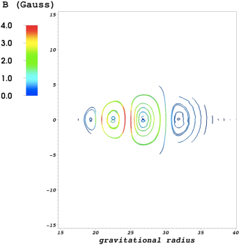
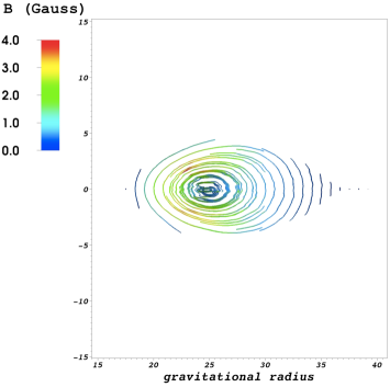
Figure 1: Initial magnetic field configuration for the four poloidal loop case (top panel) and the single poloidal loop case (bottom panel). The colour scales with the value of the magnetic field.

The fact that $\beta_{mag,0}$ affects our final result is not surprising since our simulations do not reach a saturated (magnetically arrested or magnetically choked) state (Igumenshchev et al., 2003; Igumenshchev, 2008; Tchekhovskoy et al., 2011; McKinney et al., 2012). Our resulting field strength is dictated by how much magnetic field is made available to the black hole through our initial conditions.

In the background region not specified by the torus solution, we set up a low density non-magnetic gas. Numerical floors are placed on density and energy density with the following forms: $\rho_{\rm floor}=10^{-4}\rho_{\rm max,0}r^{-1.5}$ and $e_{\rm floor}=\rho\epsilon=10^{-6}\rho_{\rm max,0}r^{-2.5}$. These floors are never applied within the disc, nor in most of the background region. They are only seldom applied very close to the outer boundary (the few last external cells), and more frequently along the vertical axis in the funnel region. The most commonly applied floor is that on the ratio $(\rho+\rho\epsilon)/P_{B}$. Whenever this quantity drops below 0.01 (almost always within the jets), both $\rho$ and $\rho\epsilon$ are rescaled by a factor appropriate to maintain this ratio.

3.2 Grid

All of the simulations are performed in 2.5 spatial dimensions (all three spatial components of vector quantities are evolved in a single azimuthal slice, although symmetry is assumed in the azimuthal direction) using a spherical polar coordinate grid. The grid used in the majority of the simulations consists of 256 radial zones and 256 zones in polar angle.

In the radial direction, we use a logarithmic coordinate of the form $\eta\equiv 1.0+\ln(r/r_{\rm BH})$, where $r_{\mathrm{BH}}=r_{G}(1+\sqrt{1-a_{*}})$ is the radius of the black hole horizon; therefore, $\Delta r/r=\mathrm{constant}$. The inner and outer radial boundaries are set at $0.9r_{\mathrm{BH}}$ and $120r_{G}$, respectively. Note that, because we use the Kerr-Schild form of the Kerr metric, we are able to place the inner radial boundary some number of zones (usually 4) inside the black hole horizon. In principle, this choice should keep the inner boundary causally disconnected from the flow, since MHD signals cannot physically radiate out from within the event horizon. This situation is preferable to having the inner boundary of the grid outside the event horizon, which can lead to artificial behavior within the flow. The spatial resolution near the black hole horizon is $\Delta r\approx 0.023r_{G}$; near the initial pressure maximum of the torus, it is $\Delta r\approx 0.45r_{G}$. We use outflow boundary conditions at both the inner and outer boundaries (the MHD primitive variables are copied from interior zones into ghost zones, except the radial velocity component, which is zeroed out if it would lead to inflow onto the grid).

Since we consider a fairly small radial range, there is some concern that our jets (discussed in Section 5.1) might be affected by reflections of waves off the outer boundary of the grid. To test this, we performed one simulation, B4S9T3M9Ce, that used an extended radial grid with $r_{\mathrm{max}}=1.1\times 10^{4}r_{G}$. We found that most properties of this simulation were very similar to the corresponding results done on the smaller (default) grid. The deviations were consistent with those expected from using a different random perturbation seed, as was the case here since the new simulation used a different processor distribution which affects the random seeding.

In the angular direction, we include the full range $0\leq\theta\leq\pi$, with reflecting boundary conditions applied at the poles (meaning that the MHD primitive variables are copied from interior zones into ghost zones, with the sign reversed on the $\theta$ component of all vector quantities, plus the staggered magnetic field component zeroed out at the pole). We use a concentrated latitude coordinate $x_{2}$ of the form $\theta=x_{2}+\frac{1}{2}(1-h)\sin(2x_{2})$ with $h=0.3$, which gives us a better resolution near the midplane ($r_{\rm center}\Delta\theta=0.1r_{G}$). Figure 2 shows the initial state of the simulation together with the grid resolution.

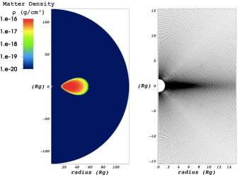
Figure 2: Initial setup of the simulation. The colour/saturation scales with the density. The number of cells scales inversely with distance from the black hole and angle away from the equatorial plane. (The left panel shows the full computational domain while the right panel only shows the region of interest closer to the central SMBH.)

Our choice of resolution is sufficient to ensure that the fastest growing poloidal field MRI modes are well resolved [$\lambda_{\mathrm{MRI}}\equiv 2\pi v_{\mathrm{A}_{z}}/\Omega\gtrsim 10\Delta z$ (Hawley et al., 2011)] for at least the first few orbits of the simulation. We also confirm that $\alpha_{\rm mag}=-B^{r}B^{\phi}/P_{B}\approx 0.3$, as expected (Hawley et al., 2011). We also performed select simulations at one-half and at double our default resolution to directly test the numerical convergence of our results (simulations B4S9l and B4S9h in Table 1). We find very little variation between our default resolution (such as in simulation B4S9) and its higher resolution counterpart (B4S9h), suggesting our results are well converged.

Since our ultimate goal is to compare spectra from our simulations with actual data, our true criterion for demonstrating reasonable convergence is to compare spectra generated from simulations at different resolutions. Figure 3 demonstrates that simulation B4S9, with a resolution of $256\times 256$, gives a spectrum that agrees with simulation B4S9h, with a resolution of $384\times 384$, to within our error bars. On the other hand, simulation B4S9l, with a resolution of $192\times 128$, produces a markedly different spectrum that diverges from the other two. Recently, Shiokawa et al. (2012) confirmed that once a certain resolution is achieved, further increases in resolution have little effect on the spectra.

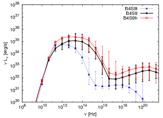
Figure 3: Median broadband spectra taken from all timesteps in the interval 2.5-3.5 orbits for 3 simulations done at different resolutions. The error bars represent the 1 sigma limits about the median (see text for more details). The spectra contain two components: the synchrotron component responsible for the first bump, and the inverse Compton component at higher frequencies.

3.3 Time interval

Because the simulations are performed assuming axial symmetry, the anti-dynamo theorem stating that an axisymmetric magnetic field cannot be maintained via dynamo action (Cowling, 1933), prevents the MRI from being self-sustaining. After an initial phase of vigorous growth of the MRI channel modes, the turbulence gradually dies out as the simulations progress. This 2D approximation is a main caveat of the simulations we have run, and it is therefore important for us to carefully choose the time interval that we wish to analyse. We want it to be after the initial phase of MRI growth, but before the mass accretion has begun to decay too dramatically (longer simulation times are not necessarily beneficial in 2D for this reason). Since we have a target mass accretion rate in mind for each simulation, we can use that as a guide for selecting our time interval.

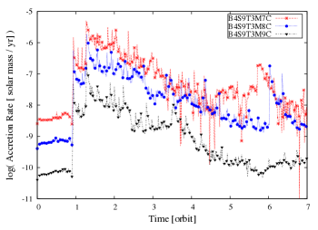
Figure 4: Mass accretion rate at the event horizon of simulations B4S9T3M9C, B4S9T3M8C, and B4S9T3M7C as a function of time.

Figure 4 shows the variation of the accretion rate as a function of time for three simulations that include cooling (B4S9T3M9C, B4S9T3M8C, and B4S9T3M7C). We see that it takes roughly 1.5 orbits to have the accretion reach its peak value, and that the accretion dies out (returns to the background rate) after about orbit 5, where we are referring to the circular orbital period at $r=r_{\rm center}$, i.e. $t_{\rm orb}=2\pi(g_{t\phi}\ell-g_{\phi\phi})/(g_{tt}\ell-g_{t\phi})=1.67\times 10^{4}~{}{\rm s}$. For these three simulations, the target accretion rates were $10^{-9}$, $10^{-8}$, and $6\times 10^{-8}M_{\odot}~{}{\rm yr^{-1}}$, respectively. Figure 4 then suggests that an appropriate interval would be between 2.5 and 3.5 orbits. We therefore use this as the standard time interval for analysis. in the rest of this paper, $2.5t_{\rm orb}=t_{\rm min}\leq t\leq t_{\rm max}=3.5t_{\rm orb}$. We confirmed that our region of interest ($r\leq 15r_{G}$) has reached inflow equilibrium over this time interval, based, for instance, on the mass flux being constant as a function of radius over this region. Therefore, we can also be confident that our selected time interval is late enough not to be affected by transient solutions.

4 Results: The importance of including cooling losses

As we have stated, our primary goal in this paper is to assess the importance of including radiative cooling losses self-consistently in numerical simulations of LLAGN like Sgr A*. We do this by comparing two types of simulations: those that include radiative cooling losses self-consistently in the dynamics (indicated by a “C” in the simulation name or cooling “ON” in Table 1) and those that neglect them (no “C”, cooling “OFF”). We performed a set of 25 different simulations to assess the importance of radiative cooling losses, as well as study the influence of parameters such as the initial magnetic field configuration, the spin, the ion to electron temperature ratio, and the mass accretion rate.

Table 1 summarizes all of the simulations performed. The name given to each simulation is derived from its parameter choices in the order they appear in the table. We also include the average and root mean square (rms) fluctuations of the mass accretion rates actually measured in our simulations. This value is to be compared with our target values of $\dot{M}$. In simulations without cooling, this value is arbitrary since the initial density (or mass) of the disc is a free parameter (other than the requirement that the total mass of the disc $M_{\rm disc}$ be negligible compared to $M_{\rm BH}$ since we ignore the self-gravity of the disc). Its choice does not affect the subsequent evolution of the simulation, so can be freely rescaled after the fact. This freedom does not extend to the simulations that include cooling, since the cooling function, $\Lambda$, depends directly on $\rho$. Therefore, to test different mass accretion rates, it is sufficient in simulations without cooling to do a single simulation and then simply rescale it to each of the target accretion rates, whereas in the simulations with cooling, a new simulation must be conducted for each new mass accretion rate. This physical scaling is an important distinction between our work and that of previous authors – each of our simulations with cooling has a real, physical mass accretion rate associated with it; it is no longer a parameter that can be freely fit to the data. When comparing simulations with cooling against those without, we always assume the same initial accretion rate.

Table 1: Description of simulation parameters

Simulation	$B$ loops ($N$)	Spin ($a_{*}$)	$T_{i}/T_{e}$	Target $\dot{M}$	statistical av. $\dot{M}$	Cooling	Resolution
B4S9T3M9C	4	0.9	3	$10^{-9}$	2.36$\pm 1.54\times 10^{-9}$	ON	$256\times 256$
B4S9T3M9Ct	4	0.9	3	$10^{-9}$	$3.05\pm 2.22\times 10^{-9}$	ON	$256\times 256$
B4S9T3M9Cb	4	0.9	3	$10^{-9}$	$1.95\pm 2.62\times 10^{-9}$	ON	$256\times 256$
B4S9T3M9Ce	4	0.9	3	$10^{-9}$	$3.00\pm 2.00\times 10^{-9}$	ON	$512\times 256$
B4S9	4	0.9	-	-	-	OFF	$256\times 256$
B1S9T3M9C	1	0.9	3	$10^{-9}$	7.93$\pm 9.27\times 10^{-9}$	ON	$256\times 256$
B1S9	1	0.9	-	-	-	OFF	$256\times 256$
B4S0T3M9C	4	0	3	$10^{-9}$	2.88$\pm 2.02\times 10^{-9}$	ON	$256\times 256$
B4S5T3M9C	4	0.5	3	$10^{-9}$	5.33$\pm 4.87\times 10^{-9}$	ON	$256\times 256$
B4S7T3M9C	4	0.7	3	$10^{-9}$	5.38$\pm 4.06\times 10^{-9}$	ON	$256\times 256$
B4S98T3M9C	4	0.98	3	$10^{-9}$	3.98$\pm 3.36\times 10^{-9}$	ON	$256\times 256$
B4S9rT3M9C	4	-0.9	3	$10^{-9}$	0.64$\pm 0.47\times 10^{-9}$	ON	$256\times 256$
B4S9T1M9C	4	0.9	1	$10^{-9}$	3.85$\pm 3.50\times 10^{-9}$	ON	$256\times 256$
B4S9T10M9C	4	0.9	10	$10^{-9}$	3.62$\pm 3.90\times 10^{-9}$	ON	$256\times 256$
B4S9l	4	0.9	-	-	-	OFF	$192\times 128$
B4S9h	4	0.9	-	-	-	OFF	$384\times 384$
B4S9T3M8C	4	0.9	3	$10^{-8}$	4.99 $\pm 3.80\times 10^{-8}$	ON	$256\times 256$
B4S9T3M7C	4	0.9	3	$6.3\times 10^{-8}$	1.69 $\pm 1.39\times 10^{-7}$	ON	$256\times 256$
B4S0T3M7C	4	0	3	$6.3\times 10^{-8}$	2.16 $\pm 1.46\times 10^{-7}$	ON	$256\times 256$
B4S5T3M7C	4	0.5	3	$6.3\times 10^{-8}$	2.03$\pm 1.85\times 10^{-7}$	ON	$256\times 256$
B4S75T3M7C	4	0.75	3	$6.3\times 10^{-8}$	1.65$\pm 1.15\times 10^{-7}$	ON	$256\times 256$
B4S98T3M7C	4	0.98	3	$6.3\times 10^{-8}$	1.37$\pm 1.08\times 10^{-7}$	ON	$256\times 256$
B4S9rT3M7C	4	-0.9	3	$6.3\times 10^{-8}$	0.39$\pm 0.41\times 10^{-7}$	ON	$256\times 256$
B4S9T1M7C	4	0.9	1	$6.3\times 10^{-8}$	1.53$\pm 1.02\times 10^{-7}$	ON	$256\times 256$
B4S9T10M7C	4	0.9	10	$6.3\times 10^{-8}$	1.43$\pm 0.88\times 10^{-7}$	ON	$256\times 256$

4.1 Effects of the cooling losses on the dynamics

Since our cooling function $\Lambda$ depends on $\rho$, $T_{e}$, and $b^{2}$ (as well as $H$), one way to assess the importance of cooling in the simulations is to observe how these quantities compare between simulations that include cooling and those that do not. Differences would indicate that the simulations with cooling are adjusting dynamically to the radiative losses. We present these comparisons in Figures 5 – 8.

Figure 5 shows the time- and shell-averaged density, $\rho$, for four different simulations: B4S9T3M9C, B4S9T3M8C, B4S9T3M7C, and B4S9. The simulation B4S9 has been scaled to three different accretion rates to be consistent with the three simulations that include cooling. A clear trend is apparent in this figure: as the mass accretion rate increases, the differences between simulations with cooling and those without also increases. At our lowest accretion rate ($\dot{M}\simeq 10^{-9}M_{\odot}~{}{\rm yr^{-1}}\simeq 10^{-8}\dot{M}_{\rm Edd}$), the differences are relatively small ($\lesssim 30$%), while at our highest accretion rate ($\dot{M}\approx 2\pi\times 10^{-8}M_{\odot}~{}{\rm yr^{-1}}\simeq 6.6\times 10^{-7}\dot{M}_{\rm Edd}$), they become more substantial ($\sim 50-70$%). Note that the apparent “bump” in density at $r\approx 15r_{G}$ is simply indicating that the initial mass reservoir (torus) has not fully redistributed itself by this time in the simulation (as $r_{\rm in}=15r_{G}$). The enhanced density associated with the cooling simulations can also be seen in Figure 6, which compares simulations B4S9 and B4S9T3M7C. With the cooling losses included, we end up with a thinner, denser disc.

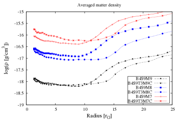
Figure 5: This figure illustrates the relative importance of radiative losses on disc density. The plot shows the averaged density for simulations B4S9T3M9C, B4S9T3M8C, B4S9T3M7C and B4S9 (rescaled to three different accretion rates). A time average is taken over the interval $t_{\rm min}-t_{\rm max}$, and at each radius we take an average over the shell.

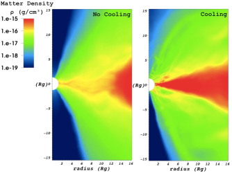
Figure 6: Time-averaged matter density (in g/cm³) of the system for simulations B4S9 and B4S9T1M7C, respectively. The simulations are initially identical; differences in the images are due entirely to cooling losses, included in the simulation in the right panel. The time average is taken over the interval $t_{\rm min}-t_{\rm max}$.

In Figure 7 we show a similar plot for the density-weighted magnetic field magnitude, $b^{2}$. Again the trend is that the differences between simulations with and without cooling become more pronounced at larger accretion rates even-though the trend is less obvious. We have a perfect match for cooling vs non cooling at the lowest accretion rate for the inner part of the disc, while the curves are distinct for the higher accretion rates. Also, the overall normalization of the magnetic field increases with mass accretion rate, which makes sense since the magnetic field is, roughly speaking, normalized by the mass density of the fluid. Further, since we are assuming ideal MHD, the magnetic field is trapped in the fluid, so as the torus spreads into a disc, the magnetic flux will be carried with it. Therefore, it is not surprising that the differences in Figure 7 are not as large as in Figure 5 for $\rho$.

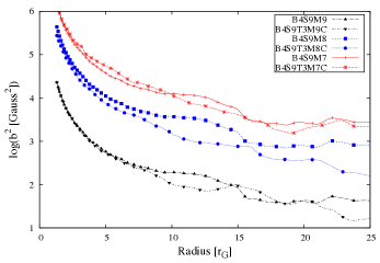
Figure 7: Plot illustrating the relative importance of radiative losses on the resulting magnetic field. The plot shows the average of $P_{B}$ for simulations B4S9T3M9C, B4S9T3M8C, B4S9T3M7C and B4S9 (rescaled to three different accretion rates). A time average is taken over the interval $t_{\rm min}-t_{\rm max}$, and at each radius we take a density-weighted average over the shell.

The density-weighted temperature (representative of the disc temperature) is shown in Figure 8, which helps illustrate one of our main conclusions in this paper. The close agreement between the non-cooling simulations and simulation B4S9T3M9C (target $\dot{M}\approx 10^{-9}M_{\odot}~{}{\rm yr^{-1}}$) suggests that at this level of accretion, radiative losses are not important. However, for $\dot{M}\gtrsim 10^{-8}M_{\odot}~{}{\rm yr^{-1}}$ i.e. $\dot{M}\gtrsim 10^{-7}\dot{M}_{Edd}$, the differences in temperatures of the discs dramatically increases, with the highest $\dot{M}$ simulation almost an order of magnitude colder than the lowest, at small radii. This result suggests that only for the very lowest luminosity AGN (Sgr A* being the only known candidate example at this time) is it reasonable to neglect radiative cooling losses in numerical simulations. Figure 9 demonstrates the dramatic difference in temperature, up to 2 order of magnitude in the region of interest (the inner disc), between our highest accretion rate simulation, B4S9T3M7C, and a simulation that neglected cooling (scaled to the same accretion rate). Note, especially, that only with cooling does any gas with $T<3\times 10^{11}~{}\mathrm{K}$ reach the black hole event horizon. When cooling is turned on, the lost radiation pressure results in a thinner disk, and this in turn compresses the gas and magnetic fields, so we end up with a thinner but denser disk in the inner part of the disk, while the temperature is much cooler due to the radiative losses.

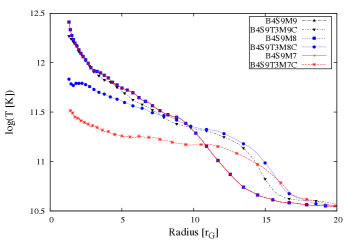
Figure 8: Plot illustrating the relative importance of radiative losses on disc temperature. The plot shows the averaged temperature for simulations B4S9T3M9C, B4S9T3M8C, B4S9T3M7C and B4S9 (rescaled to three different accretion rates). A time average is taken over the interval $t_{\rm min}-t_{\rm max}$, and at each radius we take a density-weighted average over the shell. Because the temperature does not change when the density is rescaled, the three non-cooling curves (pink, blue, and orange) are exactly on top of each other whether $\dot{M}=10^{-9},10^{-8},or\ 10^{-7}M_{\odot}~{}{\rm yr^{-1}}$

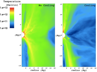
Figure 9: Time-averaged temperature (in Kelvin) of the system for simulations B4S9 and B4S9T1M7C, respectively. The simulations are initially identical; differences in the images are due entirely to cooling losses, included in the simulation in the right panel. The time average is taken over the interval $t_{\rm min}-t_{\rm max}$. Note that the system is very dynamical, with many different time scales playing themselves out. Even averaging over an orbital period does not give a perfectly symmetric system as analytic models would predict.

4.2 Effects of the cooling losses on the resulting spectra

Using numerical simulations together with spectral modeling codes to fit Sgr A* has already been considered by many authors (e.g. Goldston et al., 2005; Mościbrodzka et al., 2009; Dexter et al., 2010; Hilburn et al., 2010; Shcherbakov et al., 2010). What is new about our work is that it is the first that a numerical study of Sgr A* includes the effects of radiative cooling self-consistently.

In our companion paper (D12), we present the details of producing broadband spectra from our simulations, together with a parameter study that we use to constrain the physical environment of Sgr A*. In this paper we focus on how including cooling affects the dynamics within the simulations more generally, using sample spectra to illustrate the results. As in the previous section, we consider three different target accretion rates.

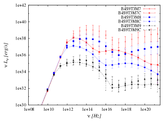
Figure 10: Broadband spectra for simulations B4S9T3M9C, B4S9T3M8C, B4S9T3M7C and B4S9 (rescaled to three different accretion rates) with an inclination angle of 85 degrees. The median is taken over the interval $t_{\rm min}-t_{\rm max}$, errors as described for Fig. 3.

Figure 10 shows the median broadband spectral energy distribution for four different simulations: B4S9T3M9C, B4S9T3M8C, B4S9T3M7C, and B4S9. The simulation B4S9 has been scaled to three different accretion rates to be consistent with the three simulations with cooling. The spectra represent the synchrotron and inverse Compton emission of the system at each frequency. They also include all special and general relativistic effects via general relativistic ray tracing using the codes geokerr (Dexter & Agol, 2009) and grtrans (Dexter, 2011). We can see that for the low accretion rates ($\dot{M}\sim 10^{-9}{\rm M_{\odot}/yr}=10^{-8}\dot{M}_{Edd}$), the spectra of simulations B4S9T3M9C and B4S9 are nearly indistinguishable, while for the high accretion rates ($\dot{M}\gtrsim 10^{-8}{\rm M_{\odot}/yr}=10^{-7}\dot{M}_{Edd}$), the spectra obtained without including the cooling losses self-consistently in the simulation are quite different than the ones where they are included. Thus, in the regime $\dot{M}\gtrsim 10^{-7}{\rm\dot{M}_{Edd}}$, we conclude that simulations which do not take cooling losses into account are likely not providing a realistic representation of the physics occurring during the accreting process. In this case, fitting for parameters such as spin, temperature ratio, magnetic filed configuration, inclination, and accretion rate is likely to yield incorrect results. This would seem to apply to all known LLAGN except perhaps Sgr A*.

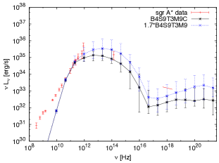
Figure 11: Broadband spectra for simulations B4S9T3M9C and B4S9 (rescaled to fit the point 230 GHz, 3 Jy) with an inclination angle of 85 degrees. The median is taken over the interval $t_{\rm min}-t_{\rm max}$. Observational data for Sgr A* are represented in red. (Falcke et al., 2000).

Of the different simulations considered in this work, the spectra of simulation B4S9T3M9C is the most compatible with the observational data of Sgr A* (see Figure 11). Note that we are not trying to fit the lowest energy data, as the radio emission is believed to be emitted from a region much further out than the radial extent of our simulation domain. In contrast, the so-called “sub-mm bump” (see, e.g., Melia & Falcke 2001) is expected to originate from quite close to the black hole, i.e. the region represented by our simulation.

To provide concrete values allowing comparison with other works, we find that we can fit the Sgr A* data at 230 GHz, which has a value of 3 Jy, or $\nu L_{\nu}\sim 4\times 10^{35}$ erg/s, with an accretion rate of $2.60\pm 1.54\times 10^{-9}{\rm M}_{\odot}$/yr via the non-scalable, cooled simulation B4S9T3M9C (see Table 1). To fit this data with the corresponding non-cooling simulation B4S9, we must scale the simulation to have an accretion rate of $2.95\pm 0.87\times 10^{-9}{\rm M_{\odot}/yr}$ at the BH horizon. These values are statistically consistent, confirming our earlier point that, at the currently best fit accretion rate, it is not necessary to consider radiative cooling processes when simulating accretion onto Sgr A*. For a complete parameter study and the best fits to Sgr A* with our models, see D12.

5 Results: parameter study

Because we have considered a fairly large parameter space in our study, we briefly report how our simulations are affected by each of these. Many of the conclusions reached in this section confirm results of earlier studies by other authors. We include them again here (with references to the earlier works) for completeness and to allow comparison.

5.1 Influence of the initial magnetic field configuration

As noted in previous studies (e.g. Beckwith et al., 2008; McKinney & Blandford, 2009), the initial magnetic field configuration has a major influence on the launching and continued powering of jets in numerical simulations. Although our study is more focused on the disc than the jets, we did make a measure of the instantaneous energy carried in the fluid and magnetic components of the jets (defined as material with $b^{2}/\rho>1$) at the time of each data writeout from our simulations. The fluid and magnetic energy of the jet are defined as

$$E_{\mathrm{FL,jet}}(t)=\int\left[\sqrt{-g}(\rho hu^{0}u_{0}+P)\right]drd\theta d\phi$$ (13)

and

$$E_{\mathrm{EM,jet}}(t)=\int\sqrt{-g}\left(2P_{B}u^{0}u_{0}+P_{B}-b^{0}b_{0}\right)drd\theta d\phi~{}.$$ (14)

Table 2 shows these quantities, averaged over the usual interval ($t_{\rm min}-t_{\rm max}$), for a subset of our simulations. We also report the same measure of jet efficiency as Tchekhovskoy et al. (2011), namely $\eta=(\dot{M}-\dot{E})/\langle\dot{M}\rangle$, where

$$\dot{M}(t)=-\int\sqrt{-g}\rho u^{r}d\theta d\phi$$ (15)

is the mass accretion rate and

$$\dot{E}(t)=\int\sqrt{-g}T_{t}^{r}d\theta d\phi~{}$$ (16)

is the energy flux, both taken at the black hole event horizon $r_{\mathrm{BH}}$. Angle brackets indicate a time-averaged quantity. The negative sign in equation (15) indicates that the mass flux is positive when rest mass is transported into the black hole. Similarly, $\dot{E}$ is constructed such that a positive value indicates a net flux of energy into the black hole.

Table 2: Jet energies and efficiencies

	$E_{\mathrm{FL,jet}}$	$E_{\mathrm{EM,jet}}$	$\eta$
Simulation	(erg)	(erg)
B4S9rT3M9C	$3.43\times 10^{38}$	$6.23\times 10^{38}$	0.225
B4S0T3M9C	$1.40\times 10^{39}$	$1.88\times 10^{39}$	0.0625
B4S5T3M9C	$7.23\times 10^{39}$	$9.80\times 10^{39}$	0.120
B4S7T3M9C	$5.50\times 10^{39}$	$1.07\times 10^{40}$	0.161
B4S9T3M9C	$1.03\times 10^{40}$	$2.19\times 10^{40}$	0.464
B1S9T3M9C	$1.07\times 10^{41}$	$6.47\times 10^{41}$	0.559
B4S98T3M9C	$1.72\times 10^{40}$	$7.60\times 10^{41}$	0.525

In our models we start with a relatively weak ($\leq 17.5{\rm G}$) magnetic field contained entirely within the disc, initially in the form of poloidal loops. We tested two different configurations: a single set of poloidal loops centered on the pressure maximum of the torus and following contours of pressure/density (an example is simulation B1S9T3M9C) and four sets of poloidal loops spaced radially, with alternating field directions in each successive loop (an example is simulation B4S9T3M9C).

The 1-loop configuration yields a significantly more energetic outflow (mostly associated with the “jets”) – more than an order of magnitude stronger than for the more complex, though perhaps more realistic, configuration consisting of 4 initial loops. We have confirmed that, as expected, the overall power of both components scales roughly linearly with the mass accretion rate, meaning the efficiencies of the outflows are not strongly effected by the cooling.

Aside from the outflow, the initial magnetic field configuration also has a strong influence on the accretion rate as seen by comparing the measured $\dot{M}$ in Table 1 for simulations B4S9T3M9C and B1S9T3M9C. The 1-loop simulation has a substantially higher average $\dot{M}$, as well as much larger statistical fluctuations. This difference is likely a consequence of the axisymmetric nature of these simulations. In our simulations, accretion is driven by the MRI. For the 1-loop case, the dominant channel solution is able to disrupt nearly the entire disc, driving large amounts of material onto the black hole in multiple short, intense episodes. In the 4-loop cases, the channel solutions are restricted in their radial range and can not disrupt the disc as effectively; accretion proceeds more smoothly, and at an overall lower normalization. [The channel solution (Hawley & Balbus, 1992) is a particularly violent form of the poloidal MRI and is characterized by prominent radially extended features.] These effects are illustrated in Figure 12.

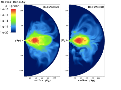
Figure 12: Density (in $g/cm^{3}$) of the system for simulations B1S9T3M9C and B4S9T3M9C at the same time step (t= 3 orbits). The two simulations started with the same initial torus configuration as shown in figure 2. The only initial difference between the two models is that the left panel started with a single magnetic loop configuration (as shown in the bottom panel of figure 1), while the right panel started with a 4 magnetic loop configuration (as shown in the top panel of figure 1). We can see that in the case of the single initial magnetic loop, the channel solution extends through the entire disc, resulting in a higher mass accretion rate at the black hole horizon and a more extended disk.

Figure 13 compares the spectra for the two different initial magnetic field configurations, the “1-loop” configuration (in black), and the “4-loop” configuration (in red) . It is clear that the magnetic field configuration has a strong influence on the resulting spectra and is therefore one of the big uncertainties affecting all such models of the accretion flow. The lack of a priori knowledge of the field configuration introduces an effective error in all simulation conclusions that is comparable to the difference introduced by including cooling. Thus, while we can treat the cooling losses self-consistently, it is difficult to overcome the variations that different choices in initial magnetic field configurations will introduce.

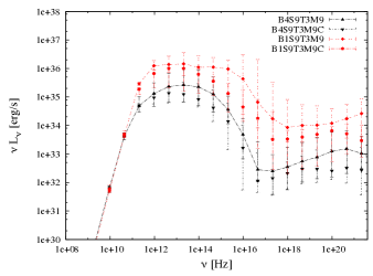
Figure 13: Broadband spectra for simulations B4S9T3M9C, B4S9T3M9, B1S9T3M9C, and B1S9T3M9. The median is taken over the interval $t_{\rm min}-t_{\rm max}$.

5.2 Influence of the Spin

Via its formation and accretion history, Sgr A* is likely a rotating SMBH, but as with all black holes it is currently difficult to reliably determine its spin. Although the observed spectrum should depend on spin, it also depends on the mass accretion rate, which is somewhat constrained, as well as the geometry of the accretion flow. Nevertheless, spectral fitting of Sgr A* has already placed some meaningful constraints on the value of $a_{*}$ (Broderick et al., 2011; Shcherbakov et al., 2010), although there can be additional complicating factors, such as disk tilt (Dexter & Fragile, 2011, 2012). Other methods of inferring the ISCO, and then the spin, such as observing relativistically-broadened line profiles or modeling the thermal emission from the disc, require the presence of a geometrically thin, optically thick disc, which is not observed at the low accretion rates of Sgr A*. The ultimate determination of spin will likely require future observations from mm-VLBI (Doeleman et al., 2008; Fish et al., 2011; Broderick et al., 2011).

Figure 14: Jet fluid energy as a function of spin. The six data points represent the averaged jet energies for B4S9rT3M9C, B4S0T3M9C, B4S5T3M9C, B4S7T3M9C, B4S9T3M9C, and B4S98T3M9C.

Figure 15: Jet magnetic energy as a function of spin. The six data points represent the averaged jet energies for B4S9rT3M9C, B4S0T3M9C, B4S5T3M9C, B4S7T3M9C, B4S9T3M9C, and B4S98T3M9C.

We investigated the spin dependence of our results by performing simulations at six different values of $a_{*}$: -0.9, 0, 0.5, 0.75, 0.9, and 0.98, where the minus sign indicates retrograde rotation (disc and black hole rotating in opposite senses). We will discuss the effects of spin on our spectral fits in companion paper D12. Concerning the disc evolution, there does not seem to be any clear trend in $\dot{M}$, see Table 1. If anything there appears to be a peak in the distributions, with the highest mass accretion rates occurring at intermediate spins, $0.3\lesssim a_{*}\lesssim 0.7$. The outflow power on the other hand, shown in Table 2, reveals a clear trend with spin, as expected based on theoretical grounds (e.g. Blandford & Znajek, 1977; Tchekhovskoy et al., 2010) and from previous numerical work (De Villiers et al., 2005; Hawley & Krolik, 2006; McKinney, 2006; Tchekhovskoy & McKinney, 2012). This trend is seen in both the fluid and magnetic components of the outflow and the correlations are shown in Figure 14.

The effect of spin on jet power is a question that has been debated recently in the literature, specifically using claimed spin observations from black hole X-ray binaries. So far the observational results are not definitive (see, e.g., the opposing conclusions found in Fender et al. 2010 and Narayan & McClintock 2012). Our results, while focusing on SMBHs, would be predicted to scale to smaller mass black hole systems via the Fundamental Plane of BH accretion relation (Merloni et al., 2003; Falcke et al., 2004). Semi-analytical models for the compact jets observed in weakly accreting systems predict a dependance of radio luminosity on total jet power of $\sim Q_{j}^{1.4}$ (e.g., Falcke & Biermann, 1995). Thus if we consider the total power as the sum of the fluid and magnetic components in Figure 15, we would also predict a correlation between observed radiative power and spin.

5.3 Disk Thickness

In all our simulations we started with the same disk thickness ($\Delta r/r=$constante $\simeq 1$) in order to start with a thick disk, appropriate for the Galactic center. Then the shape of the disk is modified during the simulation and is especially sensitive to the cooling as shown in figure 6. We also investigated thinner disk simulation, the thinner disk emmit a little bit less that the thick disk but they could be compatible within one sigma.

6 Conclusions

For the first time we have been able to assess the importance of the radiative losses in numerical simulations of LLAGN, specifically Sgr A* [see also Mościbrodzka et al. (2011)]. We show that radiative losses can affect the dynamics of the system and that their importance increases with accretion rate. We set a rough limit of $\dot{M}\gtrsim 10^{-7}\dot{M}_{\rm Edd}$, above which radiative cooling losses should be included self-consistently in numerical simulations. Otherwise, many important derived dynamical quantities, such as density, magnetic field magnitude, and temperature, may be off by an order of magnitude or more, especially when the accretion rate reaches $\dot{M}\simeq 10^{-6}\dot{M}_{\rm Edd}$, which correspond to $10^{-7}M_{\odot}~{}{\rm yr^{-1}}$ for Sgr A*. Since several recent works suggest that accretion physics is similar across the mass scale, this accretion rate in Eddington units should likely be an important limit for all black holes. Thus, we predict that the inclusion of self-consistent radiative cooling above $\sim 10^{-6}M_{\rm Edd}$ should be important for LLAGN in general.

Overall, this study allows us to have a more consistent model of accretion, even for the well-studied and under-luminous source, Sgr A*. Not only do we have a more realistic model by including the physics of radiative losses, but we are also able to show the influence of the accretion rate on the resulting spectra.

The spin of the central black hole and the initial magnetic field configuration of the torus also have important consequences on the dynamics of the system and the resulting spectra. By including the cooling losses in our study, we can discuss the influence of these free parameters with more accuracy. For instance, initial magnetic field configurations consisting of a single set of poloidal loops result in significantly more powerful outflows than the four-loop cases, and we find that the jet power increases with the spin of the central black hole.

As mentioned in Section 3.3, there is concern as to whether or not our simulations have run long enough to reach meaningful equilibrium states. This concern is especially pertinent for our case using 2.5D simulations, as these can never truly reach a steady state. The reason is that, after a period of initial vigorous growth, the MRI in 2.5D simulations steadily decays because the dynamo action that normally sustains it requires access to non-axisymmetric modes that are obviously inaccessible. We, therefore, chose a time interval for analysis when the mass accretion rate closely approximated our target value for most simulations. Clearly simulations in 3D with a longer duration (to ensure a proper equilibrium is reached) would be beneficial, for comparison.

One other concern with only performing 2.5D, axisymmetric simulations is that it precludes the possibility of exploring the effects of misalignment between the angular momentum of the gas and the black hole. In reality, most supermassive black holes are unlikely to be accreting from matter sharing the same orbital plane as the black hole spin. Dexter & Fragile (2012) recently showed that accounting for such a “tilted” accretion flow can dramatically alter the best-fit characteristics of Sgr A* and produce important new features in the spectra.

As a final note, one can justify neglecting full radiative transfer in simulations of Sgr A* and likely most other weakly accreting LLAGN because the inner regions are generally thought to be optically thin. However, to treat the outer regions of the accretion flow, or higher luminosity sources, a more thorough treatment of radiative transfer will need to be implemented into the simulations. Similarly, to approach important questions such as the mass loading and particle acceleration in the jets, likely resistive (non-ideal) MHD will need to be considered. We see this work as an important step towards these next technological “horizons”.

References

- Aitken et al. (2000) Aitken D. K., Greaves J., Chrysostomou A., Jenness T., Holland W., Hough J. H., Pierce-Price D., Richer J., 2000, ApJ, 534, L173
- Anninos & Fragile (2003) Anninos P., Fragile P. C., 2003, ApJS, 144, 243
- Anninos et al. (2005) Anninos P., Fragile P. C., Salmonson J. D., 2005, ApJ, 635, 723
- Baganoff et al. (2003) Baganoff F. K., Maeda Y., Morris M., Bautz M. W., Brandt W. N., Cui W., Doty J. P., Feigelson E. D., Garmire G. P., Pravdo S. H., Ricker G. R., Townsley L. K., 2003, ApJ, 591, 891
- Balbus & Hawley (1991) Balbus S. A., Hawley J. F., 1991, ApJ, 376, 214
- Balick & Brown (1974) Balick B., Brown R. L., 1974, ApJ, 194, 265
- Beckwith et al. (2008) Beckwith K., Hawley J. F., Krolik J. H., 2008, ApJ, 678, 1180
- Blandford & Znajek (1977) Blandford R. D., Znajek R. L., 1977, MNRAS, 179, 433
- Bower et al. (2003) Bower G. C., Wright M. C. H., Falcke H., Backer D. C., 2003, ApJ, 588, 331
- Broderick et al. (2011) Broderick A. E., Fish V. L., Doeleman S. S., Loeb A., 2011, ApJ, 735, 110
- Chakrabarti (1985) Chakrabarti S. K., 1985, ApJ, 288, 1
- Cowling (1933) Cowling T. G., 1933, MNRAS, 94, 39
- De Villiers et al. (2005) De Villiers J.-P., Hawley J. F., Krolik J. H., Hirose S., 2005, ApJ, 620, 878
- Dexter (2011) Dexter J., 2011, PhD thesis, University of Washington
- Dexter & Agol (2009) Dexter J., Agol E., 2009, ApJ, 696, 1616
- Dexter et al. (2009) Dexter J., Agol E., Fragile P. C., 2009, ApJ, 703, L142
- Dexter et al. (2010) Dexter J., Agol E., Fragile P. C., McKinney J. C., 2010, ApJ, 717, 1092
- Dexter et al. (2012) Dexter J., Agol E., Fragile P. C., McKinney J. C., 2012, ArXiv e-prints
- Dexter & Fragile (2011) Dexter J., Fragile P. C., 2011, ApJ, 730, 36
- Dexter & Fragile (2012) Dexter J., Fragile P. C., 2012, ArXiv e-prints
- Doeleman et al. (2009) Doeleman S., Agol E., Backer D., Baganoff F., Bower G. C., Broderick A., Fabian A., Fish V., Gammie C., Ho P., Honman M., Krichbaum T., Loeb A., Marrone D., Reid M., Rogers A., et al. 2009, in astro2010: The Astronomy and Astrophysics Decadal Survey Vol. 2010 of Astronomy, Imaging an Event Horizon: submm-VLBI of a Super Massive Black Hole. p. 68
- Doeleman et al. (2008) Doeleman S. S., Weintroub J., Rogers A. E. E., Plambeck R., Freund R., Tilanus R. P. J., Friberg P., Ziurys L. M., Moran J. M., Corey B., Young K. H., Smythe D. L., Titus M., Marrone D. P., Cappallo R. J., Bock D. C.-J., et al. 2008, Nat., 455, 78
- Esin et al. (1996) Esin A. A., Narayan R., Ostriker E., Yi I., 1996, ApJ, 465, 312
- Falcke & Biermann (1995) Falcke H., Biermann P. L., 1995, A&A, 293, 665
- Falcke et al. (2004) Falcke H., Körding E., Markoff S., 2004, A&A, 414, 895
- Falcke et al. (2000) Falcke H., Melia F., Agol E., 2000, ApJ, 528, L13
- Fender et al. (2010) Fender R. P., Gallo E., Russell D., 2010, MNRAS, 406, 1425
- Fish et al. (2011) Fish V. L., Doeleman S. S., Beaudoin C., Blundell R., Bolin D. E., Bower G. C., Chamberlin R., Freund R., Friberg P., Gurwell M. A., Honma M., Inoue M., Krichbaum T. P., Lamb J., et al. 2011, ApJ, 727, L36
- Fragile et al. (2012) Fragile P. C., Gillespie A., Monahan T., Rodriguez M., Anninos P., 2012, ApJS, ”submitted”
- Fragile & Meier (2009) Fragile P. C., Meier D. L., 2009, ApJ, 693, 771
- Gammie et al. (2003) Gammie C. F., McKinney J. C., Tóth G., 2003, ApJ, 589, 444
- Genzel et al. (2010) Genzel R., Eisenhauer F., Gillessen S., 2010, Reviews of Modern Physics, 82, 3121
- Ghez et al. (2008) Ghez A. M., Salim S., Weinberg N. N., Lu J. R., Do T., Dunn J. K., Matthews K., Morris M. R., Yelda S., Becklin E. E., Kremenek T., Milosavljevic M., Naiman J., 2008, ApJ, 689, 1044
- Gillessen et al. (2009) Gillessen S., Eisenhauer F., Fritz T. K., Bartko H., Dodds-Eden K., Pfuhl O., Ott T., Genzel R., 2009, ApJ, 707, L114
- Goldston et al. (2005) Goldston J. E., Quataert E., Igumenshchev I. V., 2005, ApJ, 621, 785
- Harten et al. (1983) Harten A., Lax P., van Leer 1983, in SIAM review Vol. 25 of Society for Industrial and Applied Mathematics, On upstream differencing and Godunov type methods for hyperbolic conservation laws. pp 35–61
- Hawley & Balbus (1992) Hawley J. F., Balbus S. A., 1992, ApJ, 400, 595
- Hawley et al. (2011) Hawley J. F., Guan X., Krolik J. H., 2011, ApJ, 738, 84
- Hawley & Krolik (2006) Hawley J. F., Krolik J. H., 2006, ApJ, 641, 103
- Hilburn et al. (2010) Hilburn G., Liang E., Liu S., Li H., 2010, MNRAS, 401, 1620
- Hioki & Maeda (2009) Hioki K., Maeda K.-I., 2009, Phys. Rev. D, 80, 024042
- Igumenshchev (2008) Igumenshchev I. V., 2008, ApJ, 677, 317
- Igumenshchev et al. (2003) Igumenshchev I. V., Narayan R., Abramowicz M. A., 2003, ApJ, 592, 1042
- Marrone et al. (2007) Marrone D. P., Moran J. M., Zhao J.-H., Rao R., 2007, ApJ, 654, L57
- McKinney (2006) McKinney J. C., 2006, MNRAS, 368, 1561
- McKinney & Blandford (2009) McKinney J. C., Blandford R. D., 2009, MNRAS, 394, L126
- McKinney et al. (2012) McKinney J. C., Tchekhovskoy A., Blandford R. D., 2012, ArXiv e-prints
- Melia & Falcke (2001) Melia F., Falcke H., 2001, ARA&A, 39, 309
- Merloni et al. (2003) Merloni A., Heinz S., di Matteo T., 2003, MNRAS, 345, 1057
- Mościbrodzka et al. (2011) Mościbrodzka M., Gammie C. F., Dolence J. C., Shiokawa H., 2011, ApJ, 735, 9
- Mościbrodzka et al. (2009) Mościbrodzka M., Gammie C. F., Dolence J. C., Shiokawa H., Leung P. K., 2009, ApJ, 706, 497
- Narayan & McClintock (2012) Narayan R., McClintock J. E., 2012, MNRAS, 419, L69
- Noble et al. (2006) Noble S. C., Gammie C. F., McKinney J. C., Del Zanna L., 2006, ApJ, 641, 626
- Reid (1993) Reid M. J., 1993, ARA&A, 31, 345
- Schödel et al. (2002) Schödel R., Ott T., Genzel R., Hofmann R., Lehnert M., Eckart A., Mouawad N., Alexander T., Reid M. J., Lenzen R., Hartung M., Lacombe F., Rouan D., Gendron E., Rousset G., Lagrange A.-M., Brandner W., et al. 2002, Nat., 419, 694
- Schoedel et al. (2011) Schoedel R., Morris M. R., Muzic K., Alberdi A., Meyer L., Eckart A., Gezari D. Y., 2011, ArXiv e-prints
- Shcherbakov et al. (2010) Shcherbakov R. V., Penna R. F., McKinney J. C., 2010, ArXiv e-prints
- Shiokawa et al. (2012) Shiokawa H., Dolence J. C., Gammie C. F., Noble S. C., 2012, ApJ, 744, 187
- Stone & Gardiner (2009) Stone J. M., Gardiner T., 2009, Nat., 14, 139
- Tchekhovskoy & McKinney (2012) Tchekhovskoy A., McKinney J. C., 2012, MNRAS, p. L445
- Tchekhovskoy et al. (2010) Tchekhovskoy A., Narayan R., McKinney J. C., 2010, ApJ, 711, 50
- Tchekhovskoy et al. (2011) Tchekhovskoy A., Narayan R., McKinney J. C., 2011, MNRAS, 418, L79