A comparison of broad iron emission lines in archival data of
neutron star low-mass X-ray binaries

Abstract

Relativistic X-ray disk-lines have been found in multiple neutron star low-mass X-ray binaries, in close analogy with black holes across the mass-scale. These lines have tremendous diagnostic power and have been used to constrain stellar radii and magnetic fields, often finding values that are consistent with independent timing techniques. Here, we compare CCD-based data from Suzaku with Fe K line profiles from archival data taken with gas-based spectrometers. In general, we find good consistency between the gas-based line profiles from EXOSAT, BeppoSAX and RXTE and the CCD data from Suzaku, demonstrating that the broad profiles seen are intrinsic to the line and not broad due to instrumental issues. However, we do find that when fitting with a Gaussian line profile, the width of the Gaussian can depend on the continuum model in instruments with low spectral resolution, though when the different models fit equally well the line widths generally agree. We also demonstrate that three BeppoSAX observations show evidence for asymmetric lines, with a relativistic disk-line model providing a significantly better fit than a Gaussian. We test this by using the posterior predictive p-value method, and bootstrapping of the spectra to show that such deviations from a Gaussian are unlikely to be observed by chance.

1. Introduction

Broad iron emission lines are known to be prominent in the X-ray spectra of many accreting objects, especially in stellar-mass and supermassive black holes (for a review, see Miller, 2007). The highest quality X-ray observations suggest that a clear asymmetry is seen in the line profile, as would be expected if the lines originate from the innermost region of the accretion disk and therefore subject to strong relativistic effects. An origin in the innermost, relativistic regions of the accretion disk is the favored explanation for the broad lines seen in black hole X-ray binaries and AGN (for example, see reviews by Fabian et al., 2000; Reynolds & Nowak, 2003; Miller, 2007, and references therein). This interpretation has held up to many alternative models for line broadening and the nature of the innermost accretion flow (e.g., Reynolds & Wilms, 2000; Reynolds et al., 2009; Fabian et al., 2009; Miller et al., 2010).

In neutron star low-mass X-ray binaries (LMXBs), iron emission lines were first discovered in the mid-1980s with EXOSAT and Tenma (White et al., 1985, 1986; Hirano et al., 1987) and have been observed by every other major X-ray mission since (e.g. RXTE, ASCA, BeppoSAX, Chandra, XMM-Newton and Suzaku). Compared to the lines in black hole X-ray binaries and AGN, the lines seen in neutron star LMXBs are typically much weaker, with a peak deviation from the continuum of less than 10%. This likely hindered the detection of relativistic lines in neutron stars, which are otherwise expected since the potential around a neutron star is somewhat similar to that around a black hole with a low spin parameter.

Recently, sensitive CCD-based spectroscopy with Suzaku and XMM-Newton has started to probe the line shape in neutron star LMXBs (Bhattacharyya & Strohmayer, 2007; Cackett et al., 2008, 2009, 2010; Papitto et al., 2009; Reis et al., 2009; D’Aì et al., 2009, 2010; Di Salvo et al., 2009; Iaria et al., 2009; Egron et al., 2011). In many cases, relativistic line shapes are found with inner disk radii, measured using relativistic line models, close to expectations for the stellar radius. Moreover, neutron star magnetic field strength estimates based on the inner disk radius for two accreting pulsars are consistent with measurements from timing (Cackett et al., 2009; Miller et al., 2011; Papitto et al., 2009, 2011). Gas spectrometer observations have also revealed relativistic lines in 4U 1705$-$44 (Piraino et al., 2007; Lin et al., 2010).

For bright sources, photon pile-up can affect CCD spectra (Ballet, 1999; Davis, 2001). Pile-up occurs when more than one photon arrives in an event box in a single detector frame time. Thus, rather than recording the energy and time of each individual photon, all photons arriving at that location within a single frame time get counted as a single photon, with an energy equal to the sum of the energy of the individual photons (see Davis, 2001; Miller et al., 2010, for a more detailed discussion of this effect). Therefore, the shape of the detected spectrum is altered, with the spectrum becoming artificially stronger at higher energies and weaker at lower energies. This could, of course, alter the ability to accurately recover the iron K emission line profile in observations strongly affected by this process. In order to address this issue, Miller et al. (2010) performed a wide range of simulations based on typical black hole and neutron star LMXB spectra. These authors found that pile-up does not broaden the line profiles recovered, and in the most extreme cases it acts in the opposite sense, leading to a narrower line profile.

An analysis of XMM-Newton spectra of neutron star LMXBs by Ng et al. (2010) came to an opposite conclusion about how pile-up affects the line profiles. These authors looked at XMM-Newton spectra taken in pn timing mode, where the detector is read out continuously, and found that pile-up was significant in many of the observations. To mitigate these effects, they extracted spectra only from the wings of the point-spread function (PSF), excluding the columns on the detector where the count rate was highest and thus has the most severe problems. They find that the resulting spectra are consistent with a Gaussian line profile, and that relativistic, asymmetric line models are not required to fit the data. These results differ from those obtained with Suzaku, wherein excising successive annular regions of the PSF yields highly consistent and relativistic line profiles (Cackett et al., 2010). Although Ng et al. (2010) note that continuum modeling, background subtraction, charge transfer inefficiencies, and X-ray loading of offset maps (an instrumental effect that is unique to the EPIC-pn camera) have a significant effect on the overall line profile, Ng et al. (2010) conclude that photon pile-up falsely leads to relativistic line profiles. However, in the spectra excluding the core of the PSF, the quality of the spectra are severely limited as the vast majority of source counts are excluded.

In order to place new results from CCD spectroscopy of Fe K lines in neutron stars into a broader context, and in order to better understand the results of data from CCD and gas spectrometers, we systematically compare data from three gas spectrometer missions that are unaffected by pile-up (EXOSAT, RXTE, BeppoSAX) with CCD data from Suzaku. We choose to compare with the Suzaku data, because, as discussed in length by Miller et al. (2010), pile-up is much less of a problem with the Suzaku/XIS detectors than with XMM-Newton/pn – the much broader PSF of Suzaku means that the source flux is spread over many more pixels. As shown by Cackett et al. (2010), extracting the source spectrum from an annulus, excluding the central core of the Suzaku PSF, does not change the shape of the line profile obtained. In this paper, we show that the gas spectrometer data give good consistency between the different missions and with the CCD Suzaku data, supporting the relativistic interpretation of the iron line origin.

2. Data sample and reduction

In this paper, we analyze data from four different missions: EXOSAT, RXTE, BeppoSAX, and Suzaku. The detectors we utilize from EXOSAT, RXTE and BeppoSAX are gas spectrometers, whereas the Suzaku detectors covering the Fe K line region are CCDs. The combination of both effective area and energy resolution is important for iron line spectroscopy and for the discussion of our results. The parameters for the detectors we use follows here. The EXOSAT/GSPC has an energy resolution (FWHM) of approximately 10% at 6 keV ($\sim$0.6 keV Peacock et al., 1981) and an effective area of around 150 cm² at 6 keV. The BeppoSAX/MECS instrument is very comparable to EXOSAT/GSPC, with a similar energy resolution ($\sim$0.5 keV) and effective area at 6 keV (Boella et al., 1997). The proportional counters on RXTE, however, have a significantly higher effective area (about 1300 cm² per PCU), but a significantly lower energy resolution of approximately FWHM $\sim$1 keV at 6 keV (Jahoda et al., 1996). By comparison the two working front-illuminated XIS detectors on Suzaku have a combined effective area of around 600 cm² at 6 keV, and by far the best energy resolution of the detectors considered here, at approximately 0.13 keV (Mitsuda et al., 2007).

Broadband energy coverage is also important in determining the shape of the continuum either side of the iron line region. The energy range of EXOSAT/GSPC is dependent on the gain used during the observation. Most of the observations considered here are restricted to the 2 – 16 keV range (Gain 1), though some extend to higher energies (Gain 2), but in almost all those cases the S/N drops sharply above 20 keV. For RXTE we analyze data from the PCA only, which typically gives good spectra in the range from 3 - 30 keV. BeppoSAX has several detectors to provide a broad energy coverage. Here, we used the LECS (0.5 – 3.5 keV), MECS (2 – 10 keV) and PDS (15 – 200 keV, with the upper limit dependent on S/N) to provide broad energy coverage. In the case of Suzaku, we fit the XIS detectors in the energy range 1 – 10 keV, and use the PIN hard X-ray detector to provide broad band coverage from 12 – 50 keV (with the upper limit dependent on S/N).

We restrict our choice of sources here to four sources that have consistently shown the strongest broad iron emission lines in multiple observations by different missions, namely Serpens X-1, GX 349+2, GX 17+2 and 4U 1705$-$44. We analyze every EXOSAT and BeppoSAX observations of these sources. For Suzaku  we use the Suzaku spectra analyzed by Cackett et al. (2010) here, please see that paper for details of the data reduction of those data. With RXTE many observations of each source exist. As the focus of this work is on a comparison of the line profiles from different missions, as opposed to a detailed study of the line variability in each of the sources, we choose to look at only 3 RXTE spectra of each source. The specific spectra were initially chosen to be the three single longest continuous spectra of each source, but to ensure that we sampled a range of source states, we chose other observations in some cases. See Table 2 for details of the observations analyzed here.

Table 1Details of observations analyzed

Source	Mission	Obs. No.	Obs. ID	Start date	Exp. time	Source state	References
				(dd/mm/yy)	(ksec)
Serpens X-1	EXOSAT	1	60208	08/09/85	50.5	Banana	1, 2, 3, 4
Serpens X-1	BeppoSAX	1	20835002	05/09/99	15.7/32.0/15.4	Banana	5
Serpens X-1	RXTE	1	20072-01-01-000	18/07/97	12.8	Banana	6,7
Serpens X-1	RXTE	2	20072-01-04-000	31/07/97	14.5	Banana	6,7
Serpens X-1	RXTE	3	40426-01-01-000	05/09/99	15.4	Banana	6,7
Serpens X-1	Suzaku	1	401048010	24/10/06	18/29	Banana	8,9
GX 349+2	EXOSAT	1	34067	10/09/84	18.8	NB/FB	2, 10
GX 349+2	EXOSAT	2	59605	31/08/85	65.0	NB/FB	2, 10, 11
GX 349+2	EXOSAT	3	59663	01/09/85	94.3	NB/FB	2, 10, 11
GX 349+2	BeppoSAX	1	21009001	10/03/00	15.9/44.9/22.5	FB with NB/FB vertex	12
GX 349+2	BeppoSAX	2	21240002	12/02/01	15.6/76.1/39.1	FB with NB/FB vertex	13
GX 349+2	BeppoSAX	3	212400021	17/02/01	22.7/83.4/41.0	FB with NB/FB vertex	13
GX 349+2	RXTE	1	30042-02-01-000	09/01/98	17.0	FB	14
GX 349+2	RXTE	2	30042-02-01-04	13/01/98	13.6	FB	14
GX 349+2	RXTE	3	30042-02-02-060	24/01/98	15.2	NB/FB vertex	14
GX 349+2	Suzaku	1	400003010	14/03/06	8/20	NB	8, 9
GX 349+2	Suzaku	2	400003020	19/03/06	8/24	NB	8, 9
GX 17+2	EXOSAT	1	33715	05/09/84	25.1	HB	2, 15
GX 17+2	EXOSAT	2	33781	06/09/84	26.1	HB/NB vertex	2, 15
GX 17+2	EXOSAT	3	58809	20/08/85	68.9	NB	2, 15
GX 17+2	EXOSAT	4	60698	15/09/85	42.6	HB	2, 15
GX 17+2	BeppoSAX	1	21057001	04/10/99	11.6/41.1/19.6	HB/NB	16
GX 17+2	BeppoSAX	2	210570011	05/10/99	22.0/75.2/36.9	HB/NB	16
GX 17+2	BeppoSAX	3	210570012	07/10/99	13.2/48.3/23.4	HB/NB	16
GX 17+2	BeppoSAX	4	20261011	03/04/97	2.3/10.6/4.5	HB	17
GX 17+2	BeppoSAX	5	20261012	21/04/97	1.4/6.4/2.6	HB	17
GX 17+2	RXTE	1	20053-03-02-010	07/02/97	13.7	NB	18
GX 17+2	RXTE	2	30040-03-02-010	18/11/98	13.6	FB	18
GX 17+2	RXTE	3	30040-03-02-011	18/11/98	16.2	FB	18
GX 17+2	Suzaku	1	402050010	19/09/07	5/15	NB	9
GX 17+2	Suzaku	2	402050020	27/09/07	6/18	NB	9
4U 1705$-$44	BeppoSAX	1	21292001	20/08/00	20.6/43.5/20.1	Soft	19, 20
4U 1705$-$44	BeppoSAX	2	21292002	03/10/00	15.6/47.5/20.1	Hard	20, 21
4U 1705$-$44	RXTE	1	20073-04-01-00	01/04/97	12.8	Hard
4U 1705$-$44	RXTE	2	70038-04-01-01	31/08/02	12.6	Soft
4U 1705$-$44	RXTE	3	90170-01-01-000	26/10/05	16.1	Soft
4U 1705$-$44	Suzaku	1	401046010	29/08/06	14/14	Hard	9, 21, 22
4U 1705$-$44	Suzaku	2	401046020	18/09/06	17/15	Soft	9, 21, 22
4U 1705$-$44	Suzaku	3	401046030	06/10/06	18/17	Soft	9, 21, 22

Note. — Obs. No. is the observation number that we use in order to identify the observations. The BeppoSAX exposure times are given for the LECS, MECS and PDS (in that order), while the Suzaku exposure times are the good time exposure for the individual XIS detectors and the HXD/PIN good time (in that order). Source state abbreviations: NB - normal branch, HB - horizontal branch, FB - flaring branch.

References. — (1) White et al. 1986, (2) Gottwald et al. 1995, (3) Schulz et al. 1989, (4) Seon & Min 2002, (5) Oosterbroek et al. 2001, (6) Muno et al. 2002, (7) Gladstone et al. 2007, (8) Cackett et al. 2008, (9) Cackett et al. 2010, (10) Kuulkers & van der Klis 1995, (11) Ponman et al. 1988, (12) Di Salvo et al. 2001, (13) Iaria et al. 2004, (14) Zhang et al. 1998, (15) Kuulkers et al. 1997, (16) Di Salvo et al. 2000, (17) Farinelli et al. 2005, (18) Homan et al. 2002, (19) Piraino et al. 2007, (20) Fiocchi et al. 2007, (21) Lin et al. 2010, (22) Reis et al. 2009

For EXOSAT, and BeppoSAX we used the pipeline produced spectra available from the HEASARC database. The EXOSAT/GSPC pipeline produced spectra are time-averaged, background subtracted spectra. For bursting sources, the spectra have bursts already removed. The pipeline produced spectra are provided along with the corresponding response matrices. Further details of the EXOSAT data archive are given on the HEASARC website. The BeppoSAX pipeline spectra for the LECS, MECS and PDS are used. The PDS data are already background-subtracted, for the LECS and MECS we use the appropriate background file for the 8 arcmin extraction radius used for the source spectra, along with the appropriate response matrices from September 1997. For Suzaku, see the extensive details given in Cackett et al. (2010), here we use the spectra from that paper directly. Finally, for RXTE, we use spectra from PCU2 only to provide the most reliable spectrum, with the data reduced following the standard procedures. Briefly, the standard ‘goodtime’ and ‘deadtime’ corrections are applied, selecting data when the pointing offset $<0.02^{\circ}$ and the Earth-limb elevation angle was $>10^{\circ}$. Spectra from PCU2 were extracted from the Standard 2 mode data, and 0.6% systematic errors were applied to every channel. The appropriate background model for bright sources was used and response matrices were created with the PCARSP tool.

3. Spectral fitting and analysis

Spectral fitting is performed with XSPEC v12 (Arnaud, 1996), and uncertainties are quoted at the 1$\sigma$ level of confidence throughout.

Broadband spectral fitting of neutron star LMXBs is often degenerate - a combination of several different models usually fit the data well (e.g., Barret, 2001). This is a well known problem that led to the Eastern (Mitsuda et al., 1989) versus Western (White et al., 1988) model debate. Here, we choose to explore two widely used continuum models for neutron star LMXBs in order to assess the importance of continuum choice on the iron emission line profiles. We first use a model consisting of a single-temperature blackbody, disk blackbody and power-law (if needed), which we have successfully used in the past (e.g., Cackett et al., 2008, 2010) and is based on the results of testing multiple continuum models by (Lin et al., 2007). We refer to this model as Model 1. The second model we test consists of a single-temperature blackbody, Comptonized component (comptt in xspec), and in a number of cases an additional power-law (if needed). Hereafter, we refer to this model as Model 2. This model is widely used in the literature, for instance, see Barret (2001); Di Salvo et al. (2000, 2001); Iaria et al. (2004).

In both models Galactic photoelectric absorption is included with the phabs model. We mostly leave this as a free parameter in the model. However, with the RXTE data we always fix the $N_{\rm H}$ parameter at the Dickey & Lockman (1990) values (using the HEASARC $N_{\rm H}$ tool), except for GX 17+2 where we use the $N_{\rm H}$ value determined from fitting the neutral absorption edges present Chandra gratings data (Wroblewski et al., 2008), which is found to be higher than the Dickey & Lockman (1990) value. For spectra from the other missions, only when the $N_{\rm H}$ parameters tends to 0, or becomes significantly higher than the values in the literature do we fix the $N_{\rm H}$.

Initially, we fit the iron line with a Gaussian. All parameters (line energy, width and normalization) are free parameters in the fits, though the line energy of the Gaussian is restricted to be within the 6.4 – 6.97 keV range.

Brief notes on individual observations follow. Please see Cackett et al. (2010) for notes on the Suzaku data.

3.1. EXOSAT

Ser X-1: The spectrum is fit from 2 - 16 keV. For the fits with Model 2 we find an $N_{\rm H}$ significantly higher than the Dickey & Lockman (1990) value, thus for Model 2 we fix $N_{\rm H}=4\times 10^{21}$ cm^-2. This is similar to the value found when fitting XMM-Newton spectra of Ser X-1 (Bhattacharyya & Strohmayer, 2007; Cackett et al., 2010).

GX 349+2: For all three observations we fit the data from 2 - 20 keV (above 20 keV the S/N drops quickly).

GX 17+2: We find for all observations that the spectrum turns up below 3 keV leading to too low an $N_{\rm H}$ (tending to zero). We therefore ignore below 3 keV and fix $N_{\rm H}=2.38\times 10^{22}$ cm^-2 (Wroblewski et al., 2008), this value is consistent with what we find when fitting the BeppoSAX and Suzaku observations of GX 17+2. The final observation (ObsID: 75122) has very poor calibration and there is a strong feature at 4.5 keV and between 10 – 14 keV (likely caused by variations in intrinsic detector gain, a known issue with EXOSAT). We therefore do not analyze that dataset here. For ObsID 33715 and 33781 we fit between 3 – 16 keV. For ObsID 58809 and 60698 a different gain was used, thus we fit from 3 – 20 keV (above 20 keV the S/N drops).

4U 1705$-$44: We find no clear line detection in any of the observations. Upper limits on the line intensity are comparable or greater than the line intensities seen with other missions, indicating that the spectra do not have the sensitivity to detect the Fe line. The strongest evidence for a line is in ObsID 60407 which is shown in Figure 1 (bottom right hand panel, red). However, the Gaussian component in this observation is required at less than the 2$\sigma$ level. We therefore do not consider these data any further here.

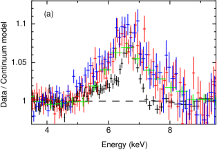
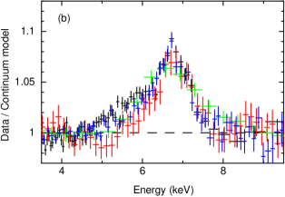
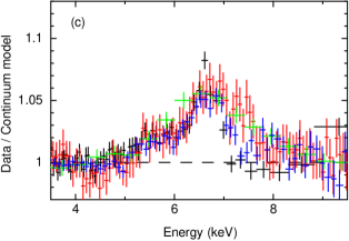
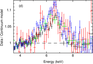
Figure 1.— A comparison of iron emission line profiles from the four different missions considered here, and good agreement is seen in most cases. Panel (a) shows Serpens X-1, (b) GX 349+2, (c) GX 17+2, and (d) 4U 1705$-$44. In all panels, black is Suzaku/XIS (all FI combined), red is EXOSAT/GSPC, blue is BeppoSAX/MECS, and green is RXTE/PCA.

3.2. RXTE

Ser X-1: We fit the spectra from 3 – 20 keV.

GX 349+2: The spectra are fit from 3 – 30 keV.

GX 17+2: The spectra are again fit from 3 – 30 keV.

4U 1705$-$44: The spectra are fit from 3-25 keV for observation 2 and 3. For observation 1, where the source is in a hard state, we fit from 3 - 50 keV.

3.3. BeppoSAX

We fit the BeppoSAX spectra allowing an offset between the LECS, MECS and PDS spectra. The constant between LECS and MECS was constrained to be within 0.7 - 1.0, and the constant between the PDS and MECS was constrained to be within 0.7 - 0.95. Unless otherwise stated, we fit the LECS between 1 – 3.5 keV, the MECS from 2 – 10 keV and the PDS from 15 keV with the upper limit determined by the quality of the data at higher energies. As noted below, in several of the spectra, there is a feature at $\sim 2.6$ keV. This feature as been discussed in previous analyses of these data by Iaria et al. (2004) and Piraino et al. (2007), who fit the feature and discuss its potential origin. While the feature may be real, it occurs at a region in the spectrum of both the LECS and MECS where there is a significant change in the response of both detectors, and thus potentially instrumental. When we fit the feature with a Gaussian, we get parameters for this line that are consistent with the previous analysis of Iaria et al. (2004) and Piraino et al. (2007). Here, we choose to ignore this section of the data in the few cases where it is present, as it is not the focus of this work. This approach, or the approach of fitting it with a Gaussian lead to consistent spectral fits at better than the 1$\sigma$ level. We generally only fit the LECS data above 1 keV as we often found significantly reduced signal-to-noise there.

Ser X-1: Here, the LECS data below 1 keV is of good quality, thus we extend the spectral fitting range from 0.5 – 3.5 keV. We fit the PDS from 15 – 30 keV.

GX 349+2: We find a poor reduced chi-squared when fitting the standard MECS range due to a strong feature at around 2.6 keV in all 3 spectra. We therefore fit the MECS data from 3-10 keV in all cases. For the PDS data we fit the range 15 – 90 keV for observation 1 which has a strong hard tail (Di Salvo et al., 2000), where as for observations 2 and 3 where this hard tail is not significant (Iaria et al., 2004), we fit from 15 – 40 keV. We did not achieve any fits with $\chi^{2}_{\nu}<2$ when using Model 1.

GX 17+2: We fit the PDS from 15 – 50 keV for all 5 observations.

4U 1705-44: In observation 1 we again find significant residuals at around 2.6 keV in the LECS and MECS spectra. We therefore fit the LECS data from 1 – 2.5 keV and the MECS data from 3 – 10 keV. We fit the PDS data from 15 – 50 keV. Observation 2 displays a strong hard tail out to 100 keV and thus we fit the PDS data up to 100 keV. However, an unbroken power-law does not fit the data well, thus we use an exponentially cut-off power-law for this observation.

4. Results

Spectral fitting results are given in Tables 2 to 9, using continuum models 1 and 2 and modeling the iron line with a Gaussian. We summarize the resulting line profiles in Figure 1 where we show a comparison of the iron line profiles for the four different objects and four different missions. For each object and mission we show only one spectrum. The profiles shown here are obtained from fitting the continuum model excluding the 5 - 8 keV range, and are plotted as the ratio of the data to the continuum model. We have chosen the continuum model that gives the best (lowest $\chi^{2}$) fit. The profiles show remarkable consistency between the different missions. All observations analyzed here give a positive detection of the iron, though this is no surprise given that these sources were chosen for that specific reason. We now discuss the main findings resulting from our analysis.

Table 2Spectral fits from EXOSAT observations with the an absorbed diskbb + bbody + Gaussian model.

Source	Obs. No.	$N_{\rm H}$	Disk blackbody		Blackbody		Gaussian				$\chi^{2}$ (dof)
		$10^{22}$ cm-2	kT (keV)	norm	kT (keV)	norm	E (keV)	$\sigma$ (keV)	norm	EW (eV)
Serpens X$-$1	1	$0.40\pm 0.15$	$1.33\pm 0.07$	$61\pm 13$	$2.10\pm 0.03$	$(3.0\pm 0.1)\times 10^{-2}$	$6.43^{+0.07}_{-0.03}$	$0.72\pm 0.09$	$(6.9\pm 1.2)\times 10^{-3}$	$169\pm 36$	192.0 (183)
GX 349+2	1	$0.25\pm 0.06$	$2.09\pm 0.10$	$44\pm 7$	$2.65\pm 0.16$	$(4.1\pm 0.1)\times 10^{-2}$	$6.68\pm 0.05$	$0.47\pm 0.08$	$(1.4\pm 0.2)\times 10^{-2}$	$102^{+16}_{-9}$	127.9 (127)
GX 349+2	2	$0.60\pm 0.04$	$2.35\pm 0.05$	$29\pm 2$	$3.46\pm 0.27$	$(2.5\pm 0.5)\times 10^{-2}$	$6.40^{+0.08}$	$1.09\pm 0.09$	$(3.6\pm 0.4)\times 10^{-2}$	$221^{+32}_{-23}$	130.4 (115)
GX 349+2	3	$0.75\pm 0.05$	$2.44\pm 0.03$	$29\pm 1$	$4.39\pm 0.45$	$(1.9\pm 0.1)\times 10^{-2}$	$6.63\pm 0.10$	$0.85\pm 0.15$	$(2.5\pm 0.4)\times 10^{-2}$	$155\pm 16$	120.1 (115)
GX 17+2	1	2.38 (fixed)	$1.40\pm 0.03$	$192\pm 16$	$2.57\pm 0.02$	$0.117\pm 0.002$	$6.58\pm 0.10$	$0.80\pm 0.14$	$(1.9\pm 0.5)\times 10^{-2}$	$131\pm 23$	139.6 (185)
GX 17+2	2	2.38 (fixed)	$1.55\pm 0.04$	$151\pm 14$	$2.46\pm 0.03$	$(9.2\pm 0.4)\times 10^{-2}$	$6.68\pm 0.14$	$0.80\pm 0.26$	$(1.2\pm 0.6)\times 10^{-2}$	$81\pm 20$	157.8 (186)
GX 17+2	3	2.38 (fixed)	$1.67\pm 0.03$	$103\pm 6$	$2.54\pm 0.04$	$(5.0\pm 0.2)\times 10^{-2}$	$6.74\pm 0.08$	$0.54\pm 0.11$	$(1.2\pm 0.2)\times 10^{-2}$	$99\pm 15$	97.7 (112)
GX 17+2	4	2.38 (fixed)	$1.46\pm 0.03$	$144\pm 11$	$2.80\pm 0.02$	$0.116\pm 0.001$	$6.4^{+0.16}$	$1.87\pm 0.14$	$(5.9\pm 0.9)\times 10^{-2}$	$424^{+329}_{-278}$	202.0 (124)

Table 3Spectral fits from EXOSAT observations with the an absorbed bbody + comptt + Gaussian model.

Source	Obs. No.	$N_{\rm H}$	Blackbody		Comptonized component				Gaussian				$\chi^{2}$ (dof)
		$10^{22}$ cm-2	kT (keV)	norm	$T_{0}$ (keV)	kT (keV)	$\tau$	norm	E (keV)	$\sigma$ (keV)	norm	EW (eV)
Serpens X$-$1	1	0.40 (fixed)	$0.87_{-0.05}^{+0.19}$	$(1.1\pm 0.4)\times 10^{-2}$	$0.35_{-0.35}^{+0.11}$	$2.22\pm 0.06$	$8.6_{-1.1}^{+0.6}$	$0.57_{-0.04}^{+0.14}$	$6.42^{+0.09}$	$0.73\pm 0.10$	$(7.0\pm 1.7)\times 10^{-3}$	$173^{+77}_{-53}$	191.6 (182)
GX 349+2	1	$0.58\pm 0.32$	$1.33\pm 0.08$	$(5.1\pm 0.4)\times 10^{-2}$	$0.46\pm 0.05$	$2.47\pm 0.06$	$7.9\pm 0.5$	$1.20_{-0.05}^{+0.17}$	$6.71\pm 0.05$	$0.39\pm 0.08$	$(1.2\pm 0.2)\times 10^{-2}$	$89^{+47}_{-8}$	124.6 (125)
GX 349+2	2	$0.5(fixed)$	$1.44\pm 0.02$	$(9.1\pm 0.3)\times 10^{-2}$	$0.33_{-0.32}^{+0.05}$	$2.91\pm 0.06$	$6.8\pm 0.2$	$1.2_{-0.1}^{+13.7}$	$6.84\pm 0.05$	$0.31\pm 0.07$	$(9.7\pm 1.4)\times 10^{-3}$	$67\pm 9$	101.1 (113)
GX 349+2	3	$0.54^{+0.55}_{-0.17}$	$1.52\pm 0.03$	$(9.9\pm 0.3)\times 10^{-2}$	$0.47\pm 0.10$	$3.15\pm 0.12$	$6.0\pm 0.5$	$0.9_{-0.2}^{+0.3}$	$6.82\pm 0.06$	$0.34\pm 0.07$	$(1.0\pm 0.2)\times 10^{-2}$	$64^{+17}_{-7}$	109.9 (114)
GX 17+2	1	2.38 (fixed)	$1.11\pm 0.09$	$(2.5\pm 0.6)\times 10^{-2}$	$0.43\pm 0.09$	$3.09\pm 0.08$	$6.0\pm 0.3$	$1.6\pm 0.2$	$6.67\pm 0.12$	$0.48\pm 0.16$	$(8.8\pm 3.1)\times 10^{-3}$	$61\pm 16$	120.9 (183)
GX 17+2	2	2.38 (fixed)	$1.32\pm 0.08$	$(5.0\pm 0.6)\times 10^{-2}$	$0.51\pm 0.05$	$2.96\pm 0.14$	$5.6\pm 0.4$	$1.5\pm 0.1$	$6.75\pm 0.12$	$0.28\pm 0.23$	$4.6_{-0.1}^{+0.4}\times 10^{-3}$	$31\pm 12$	142.6 (184)
GX 17+2	3	2.38 (fixed)	$1.19\pm 0.02$	$(5.8\pm 0.2)\times 10^{-2}$	$0.25\pm 0.06$	$2.68\pm 0.04$	$6.1\pm 0.1$	$2.3\pm 0.5$	$6.79\pm 0.06$	$0.44\pm 0.09$	$(9.4\pm 1.7)\times 10^{-3}$	$79^{+175}_{-1}$	100.8 (117)
GX 17+2	4	2.38 (fixed)	$1.46\pm 0.09$	$(1.7\pm 0.2)\times 10^{-2}$	$0.24\pm 0.05$	$3.34\pm 0.05$	$5.8\pm 0.1$	$2.2\pm 0.3$	$6.79\pm 0.09$	$0.41\pm 0.11$	$(7.2\pm 1.5)\times 10^{-3}$	$55^{+248}_{-1}$	150.4 (129)

Table 4Spectral fits from RXTE observations with the an absorbed diskbb + bbody + power-law + Gaussian model.

Source	Obs. No.	$N_{\rm H}$	Disk blackbody		Blackbody		Power-law		Gaussian				$\chi^{2}$ (dof)
		$10^{22}$ cm-2	kT (keV)	norm	kT (keV)	norm	$\Gamma$	norm	E (keV)	$\sigma$ (keV)	norm	EW (eV)
Serpens X$-$1	1	0.4 (fixed)	$1.54\pm 0.03$	$49\pm 3$	$2.37\pm 0.02$	$(2.3\pm 0.1)\times 10^{-2}$	–	–	$6.51\pm 0.06$	$0.48\pm 0.12$	$(4.8\pm 0.7)\times 10^{-3}$	$104\pm 21$	27.0 (38)
Serpens X$-$1	2	0.4 (fixed)	$1.66\pm 0.04$	$50\pm 4$	$2.39\pm 0.03$	$(3.3\pm 0.2)\times 10^{-2}$	–	–	$6.51\pm 0.06$	$0.64\pm 0.11$	$(9.6\pm 1.5)\times 10^{-3}$	$138\pm 18$	25.1 (38)
Serpens X$-$1	3	0.4 (fixed)	$1.71\pm 0.04$	$41\pm 3$	$2.41\pm 0.03$	$(2.9\pm 0.2)\times 10^{-2}$	–	–	$6.51\pm 0.06$	$0.52\pm 0.12$	$(7.0\pm 1.1)\times 10^{-3}$	$110\pm 20$	18.1 (32)
GX 349+2	1	0.5 (fixed)	$1.98\pm 0.03$	$69\pm 3$	$2.64\pm 0.03$	$(6.5\pm 0.3)\times 10^{-2}$	–	–	$6.40^{+0.01}$	$1.05\pm 0.05$	$(5.9\pm 0.3)\times 10^{-2}$	$302\pm 23$	46.2 (51)
GX 349+2	2	0.5 (fixed)	$2.28\pm 0.04$	$46\pm 3$	$2.87\pm 0.06$	$(5.1\pm 0.6)\times 10^{-2}$	–	–	$6.40^{+0.02}$	$1.26\pm 0.06$	$(6.8\pm 0.4)\times 10^{-2}$	$306\pm 25$	53.4 (52)
GX 349+2	3	0.5 (fixed)	$1.77\pm 0.02$	$87\pm 4$	$2.56\pm 0.02$	$(6.4\pm 0.2)\times 10^{-2}$	–	–	$6.40^{+0.07}$	$0.82\pm 0.09$	$(2.9\pm 0.3)\times 10^{-2}$	$186\pm 18$	37.1 (51)
GX 17+2	1	2.38 (fixed)	$1.70\pm 0.01$	$130\pm 4$	$2.68\pm 0.01$	$(7.5\pm 0.2)\times 10^{-2}$	–	–	$6.51\pm 0.10$	$0.64\pm 0.13$	$(1.5\pm 0.3)\times 10^{-2}$	$86\pm 14$	45.2 (51)
GX 17+2	2	2.38 (fixed)	$2.05\pm 0.03$	$81\pm 3$	$2.76\pm 0.02$	$0.125\pm 0.004$	–	–	$6.46_{-0.06}^{+0.09}$	$0.85\pm 0.12$	$(3.9\pm 0.6)\times 10^{-2}$	$135\pm 16$	38.5 (52)
GX 17+2	3	2.38 (fixed)	$1.88\pm 0.02$	$105\pm 4$	$2.64\pm 0.02$	$(9.7\pm 0.3)\times 10^{-2}$	–	–	$6.40^{+0.05}$	$0.92\pm 0.07$	$(5.4\pm 0.4)\times 10^{-2}$	$218\pm 19$	49.0 (52)
4U 1705$-$44	1	0.8 (fixed)	$2.28\pm 0.05$	$2.7\pm 0.2$	$4.68\pm 0.01$	$(1.2\pm 0.2)\times 10^{-2}$	$0.6\pm 0.8$	$(2.1^{+9.0}_{-1.0})\times 10^{-3}$	$6.40^{+0.01}$	$0.62\pm 0.07$	$(3.0\pm 0.2)\times 10^{-3}$	$197\pm 49$	65.2 (75)
4U 1705$-$44	2	0.8 (fixed)	$1.99\pm 0.04$	$18\pm 1$	$2.62\pm 0.05$	$(1.62\pm 0.01)\times 10^{-2}$	–	–	$6.40^{+0.02}$	$0.57\pm 0.09$	$(6.7\pm 0.7)\times 10^{-3}$	$130\pm 16$	30.6 (42)
4U 1705$-$44	3	0.8 (fixed)	$1.52\pm 0.04$	$19\pm 2$	$2.27\pm 0.02$	$(1.18\pm 0.05)\times 10^{-2}$	–	–	$6.52\pm 0.07$	$0.32\pm 0.15$	$(1.6\pm 0.3)\times 10^{-3}$	$82\pm 26$	33.8 (42)

Table 5Spectral fits from RXTE observations with the an absorbed bbody + comptt + Gaussian model.

Source	Obs. ID	$N_{\rm H}$	Blackbody		Comptonized component				Gaussian				$\chi^{2}$ (dof)
		$10^{22}$ cm-2	kT (keV)	norm	$T_{0}$ (keV)	kT (keV)	$\tau$	norm	E (keV)	$\sigma$ (keV)	norm	EW (eV)
Serpens X$-$1	1	0.4 (fixed)	$1.14\pm 0.07$	$(1.3\pm 0.3)\times 10^{-2}$	$0.41_{-0.40}^{+0.14}$	$2.58\pm 0.04$	$6.0\pm 0.3$	$0.72_{-0.22}^{+28.08}$	$6.45_{-0.05}^{+0.08}$	$0.53\pm 0.15$	$(5.2\pm 1.4)\times 10^{-2}$	$110^{+139}_{-21}$	22.0 (36)
Serpens X$-$1	2	0.4 (fixed)	$1.21\pm 0.08$	$(2.1\pm 0.4)\times 10^{-2}$	$0.44_{-0.43}^{+0.15}$	$2.51\pm 0.04$	$6.8\pm 0.3$	$0.83_{-0.09}^{+20.36}$	$6.45^{+0.09}_{-0.05}$	$0.66\pm 0.14$	$(9.9\pm 2.7)\times 10^{-3}$	$138^{+94}_{-24}$	21.6 (36)
Serpens X$-$1	3	0.4 (fixed)	$1.23\pm 0.06$	$(2.0\pm 0.2)\times 10^{-2}$	$0.39_{-0.38}^{+0.25}$	$2.50_{-0.03}^{+0.11}$	$6.8\pm 0.3$	$0.82_{-0.17}^{13.80}$	$6.47\pm 0.07$	$0.53\pm 0.17$	$(7.0_{-1.0}^{+3.7})\times 10^{-3}$	$106^{+6}_{-56}$	15.7 (30)
GX 349+2	1	0.5 (fixed)	$1.36_{-0.06}^{+0.10}$	$(7.5\pm 2.3)\times 10^{-2}$	$0.59_{-0.58}^{+0.10}$	$2.64\pm 0.05$	$6.8\pm 0.8$	$1.4_{-0.1}^{+13.8}$	$6.40^{+0.20}$	$0.99_{-0.15}^{+0.09}$	$(4.9_{-2.0}^{+01.0})\times 10^{-2}$	$246_{-65}^{+94}$	36.8 (49)
GX 349+2	2	0.5 (fixed)	$1.42\pm 0.03$	$0.11\pm 0.01$	$0.40\pm 0.37$	$2.67\pm 0.03$	$7.6\pm 0.4$	$1.6_{-0.2}^{20.4}$	$6.58_{-0.18}^{+0.13}$	$0.90\pm 0.28$	$(3.0\pm 1.3)\times 10^{-2}$	$139^{+281}_{-31}$	32.4 (43)
GX 349+2	3	0.5 (fixed)	$1.25_{-0.04}^{+0.20}$	$(5.6\pm 2.1)\times 10^{-2}$	$0.56_{-0.55}^{+0.14}$	$2.65\pm 0.06$	$6.6\pm 0.7$	$1.31_{-0.06}^{+17.84}$	$6.50_{-0.03}^{+0.12}$	$0.73\pm 0.20$	$(2.5\pm 1.0)\times 10^{-2}$	$162\pm 45$	34.3 (49)
GX 17+2	1	2.38 (fixed)	$1.83\pm 0.25$	$(1.9\pm 0.8)\times 10^{-2}$	$0.73\pm 0.03$	$3.1\pm 0.2$	$4.5\pm 0.5$	$1.6\pm 0.1$	$6.40^{+0.04}$	$1.03\pm 0.09$	$(4.1\pm 0.7)\times 10^{-2}$	$228^{+74}_{-47}$	28.9 (49)
GX 17+2	2	2.38 (fixed)	$1.91\pm 0.18$	$(6.1\pm 1.3)\times 10^{-2}$	$0.72\pm 0.04$	$3.0\pm 0.1$	$5.5\pm 0.6$	$2.0\pm 0.2$	$6.40^{+0.07}$	$1.10\pm 0.10$	$(7.1\pm 1.3)\times 10^{-2}$	$248^{+73}_{-52}$	34.3 (50)
GX 17+2	3	2.38 (fixed)	$1.79\pm 0.24$	$(4.3\pm 0.9)\times 10^{-2}$	$0.75\pm 0.04$	$2.9\pm 0.1$	$5.2\pm 0.6$	$2.0\pm 0.1$	$6.40^{+0.05}$	$1.06\pm 0.08$	$(7.7\pm 1.0)\times 10^{-2}$	$318^{+72}_{-52}$	42.4 (50)
4U 1705$-$44	1	0.8 (fixed)	$1.72\pm 0.10$	$(1.7\pm 0.6)\times 10^{-3}$	$0.80\pm 0.03$	$10.7\pm 0.9$	$2.9\pm 0.2$	$(2.8\pm 0.2)\times 10^{-2}$	$6.4^{+0.02}$	$0.69\pm 0.08$	$(3.4\pm 0.4)\times 10^{-3}$	$229\pm 38$	66.1 (75)
4U 1705$-$44	2	0.8 (fixed)	$2.87_{-0.07}^{+0.78}$	$(9.6_{-6.7}^{+0.9})\times 10^{-3}$	$0.73\pm 0.02$	$2.0^{+0.3}$	$7.6\pm 0.3$	$0.62^{+0.01}_{-0.06}$	$6.40^{+0.06}$	$0.67\pm 0.10$	$(8.0\pm 1.0)\times 10^{-3}$	$158\pm 30$	27.4 (40)
4U 1705$-$44	3	0.8 (fixed)	$1.17\pm 0.08$	$(3.5\pm 0.7)\times 10^{-3}$	$0.32_{-0.31}^{+0.14}$	$2.4\pm 0.1$	$6.8\pm 0.3$	$0.35_{-0.09}^{+5.03}$	$6.45_{-0.05}^{+0.07}$	$0.34\pm 0.15$	$(1.6\pm 0.4)\times 10^{-3}$	$82_{-6}^{+5559}$	23.0 (40)

Table 6Spectral fits from BeppoSAX observations with the an absorbed diskbb + bbody + power-law + Gaussian model.

Source	Obs.	$N_{\rm H}$	Disk blackbody		Blackbody		Power-law		Gaussian				$\chi^{2}$ (dof)
		$10^{22}$ cm-2	kT (keV)	norm	kT (keV)	norm	$\Gamma$	norm	E (keV)	$\sigma$ (keV)	norm	EW (eV)
Serpens X$-$1	1	$0.62\pm 0.01$	$1.46\pm 0.02$	$51\pm 3$	$2.21\pm 0.04$	$(3.0\pm 0.1)\times 10^{-2}$	$2.98\pm 0.06$	$0.90\pm 0.05$	$6.40^{+0.01}$	$0.96\pm 0.08$	$(1.2\pm 0.2)\times 10^{-2}$	$234\pm 31$	222.2 (133)
GX 349+2	1	No fit with reduced $\chi^{2}<2$
GX 349+2	2	No fit with reduced $\chi^{2}<2$
GX 349+2	3	No fit with reduced $\chi^{2}<2$
GX 17+2	1	$2.12\pm 0.04$	$1.81\pm 0.03$	$77\pm 5$	$2.79\pm 0.02$	$(7.0\pm 0.3)\times 10^{-2}$	$2.4\pm 0.2$	$0.26_{-0.17}^{+0.32}$	$6.60\pm 0.06$	$0.53\pm 0.15$	$(9.1\pm 2.2)\times 10^{-3}$	$60\pm 8$	203.1 (119)
GX 17+2	2	$2.12\pm 0.05$	$1.87\pm 0.01$	$70\pm 2$	$2.79\pm 0.02$	$(5.9\pm 0.2)\times 10^{-2}$	$2.7\pm 0.3$	$0.27_{-0.19}^{+0.23}$	$6.70\pm 0.03$	$0.33\pm 0.05$	$(5.8\pm 0.6)\times 10^{-3}$	$40\pm 4$	231.5 (119)
GX 17+2	3	No fit with reduced $\chi^{2}<2$
GX 17+2	4	$2.27\pm 0.10$	$1.70\pm 0.06$	$74\pm 11$	$3.01\pm 0.02$	$0.104\pm 0.005$	$2.6\pm 0.1$	$1.6\pm 0.6$	$6.83\pm 0.12$	$0.97\pm 0.20$	$(2.0\pm 0.6)\times 10^{-2}$	$154\pm 48$	175.7 (120)
GX 17+2	5	$2.08\pm 0.10$	$1.72\pm 0.06$	$86\pm 12$	$2.88\pm 0.04$	$(9.8\pm 0.6)\times 10^{-2}$	$2.3\pm 0.6$	$0.3_{-0.3}^{+0.8}$	$6.50^{+0.16}_{-0.10}$	$0.72\pm 0.26$	$(1.3\pm 0.6)\times 10^{-2}$	$84\pm 29$	143.7 (120)
4U 1705$-$44	1	$1.72\pm 0.07$	$1.52\pm 0.02$	$42\pm 3$	$2.32\pm 0.03$	$(2.9\pm 0.1)\times 10^{-2}$	$2.8\pm 0.1$	$0.6\pm 0.2$	$6.4^{+0.28}$	$0.80\pm 0.05$	$(9.7\pm 0.9)\times 10^{-3}$	$191\pm 27$	162.6 (91)
4U 1705$-$44	2	$1.48\pm 0.04$	$2.03\pm 0.07$	$2.3\pm 0.3$	$4.4\pm 0.2$	$(5\pm 1)\times 10^{-3}$	$0.6_{-0.5}^{+0.2}$*	$(1.1_{-0.8}^{+1.3})\times 10^{-2}$	$6.60\pm 0.11$	$0.76\pm 0.24$	$(1.4\pm 0.5)\times 10^{-3}$	$145\pm 88$	116.2 (106)

Note. — * The second observation of 4U 1705$-$44 has a strong hard tail extending to 100 keV. A single power-law does not fit this tail well, thus we use a cut-off power-law instead. We find the cut-off energy, $E_{\rm cut}=28\pm 5$ keV.

Table 7Spectral fits from BeppoSAX observations with the an absorbed bbody + comptt + power-law + Gaussian model.

Source	Obs	$N_{\rm H}$	Blackbody		Comptonized component				Power-law		Gaussian				$\chi^{2}$ (dof)
		$10^{22}$ cm-2	kT (keV)	norm	$T_{0}$ (keV)	kT (keV)	$\tau$	norm	$\Gamma$	norm	E (keV)	$\sigma$ (keV)	norm	EW (eV)
Serpens X$-$1	1	$0.56\pm 0.05$	$0.99\pm 0.02$	$(1.4\pm 0.1)\times 10^{-2}$	$0.10\pm 0.01$	$2.58\pm 0.04$	$6.7\pm 0.1$	$2.0\pm 0.2$	–	–	$6.40^{+0.26}$	$1.01\pm 0.07$	$(1.5\pm 0.2)\times 10^{-2}$	$288_{-26}^{+40}$	226.6 (132)
GX 349+2	1	$0.52\pm 0.03$	$1.44\pm 0.02$	$(6.2\pm 0.3)\times 10^{-2}$	$0.45\pm 0.01$	$2.63\pm 0.04$	$6.7\pm 0.2$	$1.18\pm 0.03$	$2.1\pm 0.3$	$(4.8_{-3.4}^{+14.2})\times 10^{-2}$	$6.68\pm 0.03$	$0.40\pm 0.04$	$(1.1\pm 0.1)\times 10^{-2}$	$80\pm 7$	160.7 (105)
GX 349+2	2	$0.52\pm 0.01$	$0.60\pm 0.01$	$(6.2\pm 0.1)\times 10^{-2}$	$1.39\pm 0.01$	$2.94\pm 0.02$	$4.2\pm 0.1$	$1.20\pm 0.01$	–	–	$6.76\pm 0.02$	$0.20\pm 0.03$	$(5.9\pm 0.4)\times 10^{-3}$	$31\pm 3$	182.9 (100)
GX 349+2	3	$0.52\pm 0.01$	$0.62\pm 0.01$	$(6.0\pm 0.1)\times 10^{-2}$	$1.43\pm 0.01$	$3.08\pm 0.04$	$3.6\pm 0.1$	$1.00\pm 0.02$	–	–	$6.71\pm 0.02$	$0.24\pm 0.03$	$(5.9\pm 0.4)\times 10^{-3}$	$34\pm 3$	189.2 (116)
GX 17+2	1	$2.27\pm 0.09$	$1.50\pm 0.05$	$(6.6\pm 0.4)\times 10^{-2}$	$0.57\pm 0.01$	$3.10\pm 0.07$	$5.5\pm 0.3$	$0.99\pm 0.03$	$3.1\pm 0.1$	$2.6\pm 0.7$	$6.68\pm 0.04$	$0.21\pm 0.05$	$(4.0\pm 0.6)\times 10^{-3}$	$27\pm 6$	146.7 (117)
GX 17+2	2	$2.33\pm 0.10$	$1.44\pm 0.03$	$(6.8\pm 0.2)\times 10^{-2}$	$0.54\pm 0.01$	$3.01\pm 0.06$	$5.6\pm 0.2$	$1.06\pm 0.02$	$3.5\pm 0.2$	$3.0\pm 0.8$	$6.73\pm 0.03$	$0.17\pm 0.05$	$(3.3\pm 0.4)\times 10^{-3}$	$23\pm 4$	162.6 (117)
GX 17+2	3	$2.18\pm 0.10$	$1.54\pm 0.03$	$(6.6\pm 0.2)\times 10^{-2}$	$0.56\pm 0.01$	$3.18\pm 0.05$	$5.5\pm 0.1$	$1.02\pm 0.02$	$3.2\pm 0.1$	$2.0\pm 0.6$	$6.73\pm 0.05$	$0.25\pm 0.08$	$(3.1\pm 0.6)\times 10^{-3}$	$21\pm 6$	174.7 (118)
GX 17+2	4	$2.25\pm 0.17$	$1.59\pm 0.08$	$(3.2\pm 0.2)\times 10^{-2}$	$0.56\pm 0.03$	$3.37\pm 0.06$	$6.0\pm 0.2$	$0.89\pm 0.05$	$2.8\pm 0.1$	$2.6\pm 1.1$	$6.77\pm 0.06$	$0.20\pm 0.10$	$(4.3\pm 1.0)\times 10^{-3}$	$32\pm 11$	150.1 (118)
GX 17+2	5	$2.10\pm 0.29$	$1.57\pm 0.11$	$(5.3\pm 0.7)\times 10^{-2}$	$0.57\pm 0.03$	$3.25\pm 0.14$	$5.6\pm 0.4$	$0.99\pm 0.06$	$3.0\pm 0.3$	$1.8\pm 1.5$	$6.68\pm 0.10$	$0.17\pm 0.17$	$(3.3\pm 1.5)\times 10^{-3}$	$22\pm 15$	132.2 (118)
4U 1705$-$44	1	$1.57\pm 0.15$	$1.51\pm 0.03$	$(2.1\pm 0.2)\times 10^{-2}$	$0.44\pm 0.02$	$2.69\pm 0.06$	$5.9\pm 0.2$	$0.49\pm 0.03$	$2.8\pm 0.2$	$0.49\pm 0.33$	$6.56\pm 0.04$	$0.27\pm 0.06$	$(2.9\pm 0.4)\times 10^{-3}$	$58\pm 14$	141.9 (89)
4U 1705$-$44	2	$0.91_{-0.02}^{+0.28}$	–	–	$0.73\pm 0.01$	$6.65\pm 0.52$	$4.0\pm 0.1$	$(3.2\pm 0.2)\times 10^{-2}$	$-0.74^{+1.8}_{-0.8}$ *	$(1.0^{+27.2}_{-0.9})\times 10^{-3}$	$6.4^{+0.4}$	$1.12\pm 0.09$	$(3.5\pm 0.5)\times 10^{-3}$	$375_{-18}^{+81}$	115.2 (106)

Note. — * The strong hard tail extending to 100 keV requires a cut-off power-law. We find the cut-off energy, $E_{\rm cut}=20_{-3}^{+12}$ keV.

Table 8Spectral fits from Suzaku observations with the an absorbed diskbb + bbody + power-law + Gaussian model.

Source	Obs.	$N_{\rm H}$	Disk blackbody		Blackbody		Power-law		Gaussian				$\chi^{2}$ (dof)
		$10^{22}$ cm-2	kT (keV)	norm	kT (keV)	norm	$\Gamma$	norm	E (keV)	$\sigma$ (keV)	norm	EW (eV)
Serpens X$-$1	1	$0.60\pm 0.01$	$1.24\pm 0.01$	$91\pm 3$	$2.17\pm 0.02$	$(5.1\pm 0.1)\times 10^{-2}$	$2.7\pm 0.1$	$0.65\pm 0.04$	$6.65\pm 0.01$	$0.26\pm 0.02$	$(2.5\pm 0.2)\times 10^{-3}$	$44\pm 3$	1567.7 (1107)
GX 349+2	1	$0.79\pm 0.02$	$1.60\pm 0.03$	$95\pm 6$	$2.25\pm 0.02$	$0.117\pm 0.003$	$2.1\pm 0.2$	$0.17\pm 0.11$	$6.55\pm 0.03$	$0.58\pm 0.04$	$(1.4\pm 0.1)\times 10^{-2}$	$87\pm 6$	1341.9 (1108)
GX 349+2	2	$0.88\pm 0.02$	$1.50\pm 0.02$	$97\pm 4$	$2.30\pm 0.02$	$(9.5\pm 0.1)\times 10^{-2}$	$2.4\pm 0.1$	$0.44\pm 0.09$	$6.71\pm 0.02$	$0.35\pm 0.03$	$(7.5\pm 0.5)\times 10^{-3}$	$62\pm 4$	1293.6 (1108)
GX 17+2	1	$2.24\pm 0.11$	$1.77\pm 0.02$	$83\pm 4$	$2.68\pm 0.03$	$(5.9\pm 0.2)\times 10^{-2}$	$2.9\pm 0.4$	$0.84\pm 0.68$	$6.57\pm 0.05$	$0.28\pm 0.05$	$(4.3\pm 0.7)\times 10^{-3}$	$30\pm 6$	644.0 (608)
GX 17+2	2	$2.27\pm 0.07$	$1.88\pm 0.02$	$71\pm 3$	$2.64\pm 0.02$	$(7.6\pm 0.3)\times 10^{-2}$	$3.0\pm 0.2$	$1.1\pm 0.5$	$6.60\pm 0.02$	$0.21\pm 0.02$	$(5.4\pm 0.5)\times 10^{-3}$	$32\pm 4$	665.9 (608)
4U 1705$-$44	1	2.0 (fixed)	$(8.4\pm 0.8)\times 10^{-2}$	$(7.7^{+17.2}_{-5.8})\times 10^{7}$	$1.18\pm 0.06$	$(6.6\pm 0.5)\times 10^{-4}$	$1.67\pm 0.01$	$0.127\pm 0.02$	$6.55\pm 0.03$	$0.20\pm 0.03$	$(2.5\pm 0.4)\times 10^{-4}$	$41\pm 11$	961.8 (1123)
4U 1705$-$44	2	$2.01\pm 0.02$	$1.23\pm 0.02$	$44\pm 3$	$2.18\pm 0.03$	$(2.3\pm 0.1)\times 10^{-2}$	$3.0\pm 0.1$	$0.79\pm 0.05$	$6.4^{+0.1}$	$0.68\pm 0.03$	$(3.5\pm 0.3)\times 10^{-3}$	$121\pm 16$	1364.5 (1123)
4U 1705$-$44	3	$1.98\pm 0.03$	$0.74\pm 0.01$	$139\pm 15$	$1.84\pm 0.01$	$(9.8\pm 0.1)\times 10^{-3}$	$2.9\pm 0.1$	$0.38\pm 0.05$	$6.4^{+0.2}$	$0.40\pm 0.05$	$(4.5\pm 0.8)\times 10^{-4}$	$40\pm 14$	1275.8 (1122)

Table 9Spectral fits from Suzaku observations with the an absorbed bbody + comptt + power-law + Gaussian model.

Source	Obs	$N_{\rm H}$	Blackbody		Comptonized component				Power-law		Gaussian				$\chi^{2}$ (dof)
		$10^{22}$ cm-2	kT (keV)	norm	$T_{0}$ (keV)	kT (keV)	$\tau$	norm	$\Gamma$	norm	E (keV)	$\sigma$ (keV)	norm	EW (eV)
Serpens X$-$1	1	$0.57\pm 0.01$	$0.75\pm 0.01$	$(8.6\pm 0.4)\times 10^{-3}$	$0.15\pm 0.01$	$2.44\pm 0.01$	$7.8\pm 0.1$	$1.54\pm 0.09$	–	–	$6.65\pm 0.01$	$0.26\pm 0.02$	$(2.5\pm 0.1)\times 10^{-3}$	$44\pm 3$	1605.7 (1109)
GX 349+2	1	$0.55\pm 0.01$	$1.37\pm 0.07$	$(4.8\pm 0.4)\times 10^{-2}$	$0.45\pm 0.01$	$2.52\pm 0.04$	$7.9\pm 0.3$	$1.48\pm 0.04$	–	–	$6.67\pm 0.03$	$0.38\pm 0.05$	$(8.6\pm 1.1)\times 10^{-3}$	$54\pm 5$	1476.2 (1108)
GX 349+2	2	$0.93\pm 0.01$	$0.94\pm 0.01$	$(3.00\pm 0.08)\times 10^{-2}$	$0.13\pm 0.01$	$2.51\pm 0.01$	$8.31\pm 0.06$	$2.6\pm 0.1$	–	–	$6.65\pm 0.03$	$0.49\pm 0.05$	$(1.1\pm 0.1)\times 10^{-2}$	$59\pm 11$	1367.3 (1108)
GX 17+2	1	$2.55\pm 0.06$	$1.30\pm 0.04$	$(4.8\pm 0.4)\times 10^{-2}$	$0.60\pm 0.02$	$2.83\pm 0.05$	$6.1\pm 0.2$	$1.10\pm 0.02$	$3.5\pm 0.1$	$5.1\pm 0.7$	$6.54\pm 0.06$	$0.31\pm 0.07$	$(4.6\pm 1.0)\times 10^{-3}$	$32\pm 7$	618.7 (607)
GX 17+2	2	$2.50\pm 0.06$	$1.36\pm 0.05$	$(5.3\pm 0.3)\times 10^{-2}$	$0.56\pm 0.02$	$2.73\pm 0.05$	$6.8\pm 0.3$	$1.27\pm 0.02$	$3.4\pm 0.1$	$4.6\pm 0.6$	$6.60\pm 0.02$	$0.20\pm 0.03$	$(5.0\pm 0.6)\times 10^{-3}$	$30\pm 4$	637.6 (606)
4U 1705$-$44	1	$1.56\pm 0.03$	$0.96\pm 0.01$	$(2.23\pm 0.02)\times 10^{-3}$	$0.12_{-0.01}^{+0.12}$	$6.6\pm 0.1$	$5.94\pm 0.03$	$(3.5\pm 0.1)\times 10^{-2}$	–	–	$6.4^{+0.01}$	$0.87\pm 0.05$	$(1.4\pm 0.1)\times 10^{-2}$	$239_{-22}^{+485}$	1009.2 (1123)
4U 1705$-$44	2	$1.90\pm 0.01$	$0.61\pm 0.02$	$(1.9\pm 0.3)\times 10^{-3}$	$0.14\pm 0.02$	$2.54\pm 0.01$	$6.85\pm 0.07$	$1.0\pm 0.1$	–	–	$6.4^{+0.2}$	$0.60\pm 0.03$	$(2.7\pm 0.2)\times 10^{-3}$	$92\pm 15$	1368.2 (1125)
4U 1705$-$44	3	$1.59\pm 0.02$	$1.98\pm 0.03$	$(7.1\pm 0.4)\times 10^{-3}$	$0.36\pm 0.01$	$3.9\pm 0.5$	$3.1\pm 0.4$	$0.13\pm 0.02$	–	–	$6.4^{+0.1}$	$0.46\pm 0.05$	$(6.8\pm 1.0)\times 10^{-4}$	$62\pm 19$	1261.6 (1123)

4.1. Asymmetric line profiles

Our previous analysis of Suzaku data (Cackett et al., 2008, 2010) has shown evidence for asymmetric line profiles, which can be fit well by a relativistic disk line model. The iron lines in EXOSAT and BeppoSAX have been analyzed in the past (e.g., Gottwald et al., 1995; Di Salvo et al., 2001; Oosterbroek et al., 2001; Iaria et al., 2004), however, generally only a Gaussian line profile has been considered. An exception to this is the case of 4U 1705$-$44, where both Piraino et al. (2007) and Lin et al. (2010) have fitted a relativistic diskline model to BeppoSAX data, finding that it is a better fit than a simple Gaussian. Here, we also fit the iron lines with a relativistic disk-line model (diskline, Fabian et al., 1989). Of the eight EXOSAT spectra we analyze here, six show a decreased value of $\chi^{2}$ when using a diskline model rather than a Gaussian. However, in all those cases the fit with a Gaussian already provides a reduced-$\chi^{2}<1$, thus the improvement is not statistically significant. The parameters of the diskline fits are reasonable, and consistent with typical parameters (such as in Cackett et al., 2010), but are not very well constrained. In the case of BeppoSAX, a diskline generally provides equivalently good fits to the data. However, in three cases, we find that a diskline fits the data significantly better than a Gaussian.

The three cases where a diskline is a significantly better fit are GX 349+2 observation 1, GX 17+2 observation 1 and 4U 1705$-$44 observation 1. Note that the 4U 1705$-$44 observation is the same one discussed in detail by Piraino et al. (2007), who also find an improvement in $\chi^{2}$ when using a diskline compared to a Gaussian. The parameters for the diskline fits to these three spectra are given in Table 10. We give the parameters using the Model 2 continuum as these provide a better fit in all cases. A comparison between the diskline fit parameters in Table 10 with previously published fits to these sources show they are consistent. Our fits to 4U 1705-44 are consistent with similar fits performed by Piraino et al. (2007) to the same data. Furthermore, the diskline parameters we find here are all reasonable when comparing with fits to Suzaku and XMM-Newton data of GX 349+2 (Cackett et al., 2008, 2010; Iaria et al., 2009), GX 17+2 (Cackett et al., 2010) and 4U 1705-44 (Reis et al., 2009; Di Salvo et al., 2009; Cackett et al., 2010; D’Aì et al., 2010; Lin et al., 2010). In particular, the inner disk radius and equivalent width are consistent with this previous work for similar source states.

Table 10Spectral fits to BeppoSAX observations using a relativistic emission line model.

Source	Obs	$N_{\rm H}$	Blackbody		Comptonized component				Power-law		Diskline						$\chi^{2}$ (dof)
		$10^{22}$ cm-2	kT (keV)	norm	$T_{0}$ (keV)	kT (keV)	$\tau$	norm	$\Gamma$	norm	E (keV)	$\beta$	$R_{\rm in}$	$i(^{\circ})$	norm	EW (eV)
GX 349+2	1	$0.51\pm 0.02$	$1.45\pm 0.02$	$(6.0\pm 0.2)\times 10^{-2}$	$0.47\pm 0.01$	$2.63\pm 0.04$	$6.7\pm 0.2$	$1.18\pm 0.02$	$2.1\pm 0.2$	$(5.4_{-3.2}^{+5.8})\times 10^{-2}$	$6.97_{-0.35}$	$-3.0\pm 0.4$	$8.3_{-1.9}^{+1.0}$	$22_{-2}^{+8}$	$(1.2_{-0.1}^{+0.3})\times 10^{-2}$	$111\pm 13$	138.2 (103)
4U 1705$-$44	1	$1.66\pm 0.17$	$1.58\pm 0.07$	$(1.8\pm 0.3)\times 10^{-2}$	$0.48\pm 0.03$	$2.64\pm 0.12$	$6.0\pm 0.5$	$0.47\pm 0.06$	$2.9\pm 0.1$	$0.8\pm 0.5$	$6.65_{-0.25}^{+0.32}$	$-5.3^{+1.6}_{-4.7}$	$11_{-3}^{+8}$	$29\pm 6$	$(5.6\pm 0.6)\times 10^{-3}$	$120\pm 20$	113.7 (87)
GX 17+2	1	$2.33\pm 0.09$	$1.55\pm 0.06$	$(5.7\pm 0.4)\times 10^{-2}$	$0.61\pm 0.01$	$3.11\pm 0.08$	$5.4\pm 0.3$	$1.00\pm 0.04$	$3.18\pm 0.08$	$3.2\pm 0.7$	$6.47^{+0.23}$	$<-4.8$	$18^{+5}_{-9}$	$37\pm 8$	$(9.0\pm 0.9)\times 10^{-3}$	$67^{+23}_{-32}$	132.0 (115)

Note. — $R_{\rm in}$ is given in GM/c². In the diskline model, the outer disk radius is fixed at $R_{\rm out}=1000$ GM/c² in all cases.

In Figure 2 we show the line profiles with both a Gaussian and diskline model. The diskline fit to observation 1 of GX 349+2 gives an improvement of $\Delta\chi^{2}=22.6$ for 2 additional degrees of freedom. This corresponds to a F-test probability of $4.1\times 10^{-4}$, approximately a 3.5$\sigma$ significance. Observation 1 of 4U 1705$-$44 shows an decrease of $\Delta\chi^{2}=28.2$ when using a diskline model rather than a Gaussian, which corresponds to an F-test probability of $6.6\times 10^{-5}$, or 4.0$\sigma$ significance. Finally, BeppoSAX observation 1 of GX 17+2 shows a decrease of $\Delta\chi^{2}=14.7$ when using a diskline model rather than a Gaussian, which corresponds to an F-test probability of $2.3\times 10^{-3}$, or 3.0$\sigma$ significance. It is important to also take into account the number of observations we searched to find the asymmetric lines, as this will reduce the significance. In total, we compared diskline and Gaussian fits to a total of 19 observations from EXOSAT and BeppoSAX. The probabilities given above should therefore be multiplied by 19, reducing the significances to 2.7, 3.2, and 2.0 $\sigma$ for GX 349+2, 4U 1705$-$44, and GX 17+2, respectively.

Figure 2.— Line profiles from BeppoSAX observations of 4U 1705+44 (left, observation 1), GX 17+2 (center, observation 1) and GX 349+2 (right, observation 1) fit with both a Gaussian (top), and diskline (bottom). In all three cases, the diskline gives a statistically better fit.

Egron et al. (2011) discuss how under the criteria of Protassov et al. (2002), the F-test can be properly applied to comparing Gaussian and diskline fits. Egron et al. (2011) also apply the posterior predictive p-value test (ppp, Hurkett et al., 2008) as a method to determine whether a Gaussian or diskline provides a better fit. Here, we also apply this ppp test, and secondly we perform bootstrap resampling (Efron, 1979) of the spectra to further test the significance of the improvement in using the diskline model instead of a Gaussian. Essentially, the ppp test involves a Monte Carlo simulation to test the likelihood that the diskline model gives the improvement in $\chi^{2}$ by chance. First, we find the best-fitting Model 2 using a Gaussian to fit the Fe K line (we use Model 2 as it gives better fits than Model 1). Next, we simulate 1000 sets of spectra (LECS, MECS and PDS spectra for each case) with the model parameters randomly drawn using the covariance matrix of the best-fit and using the detector responses, background spectra and exposures from the real data in the simulations. These 1000 simulated spectra are then fit with the same (Gaussian) model, and also with the diskline model. The posterior predictive distribution is defined by the values of $\Delta\chi^{2}$ from comparing fits to the simulated spectra with the Gaussian and diskline models. The ppp value is then defined by the number of instances where $\Delta\chi^{2}$(simulation) $>$ $\Delta\chi^{2}$(data), see equation 12 and section 3.2 in Hurkett et al. (2008). In Figure 3 we show the posterior predictive distributions for the three cases (discussed above) where we find a significant improvement using diskline based on the F-test alone. In all three cases we do not find a single simulation with a $\Delta\chi^{2}$ greater than as measured by the data. Given that we find zero instances where $\Delta\chi^{2}$(simulation) $>$ $\Delta\chi^{2}$(data) we cannot directly calculate a ppp value. However, we can infer that the confidence level indicated by the results corresponds to better than 99.9% level (i.e. less than 1 occurrence in 1000 simulations), which indicates an improvement at better than the 3.29$\sigma$ level. Thus, the simulations strongly support the F-test results that a diskline is the preferred model.

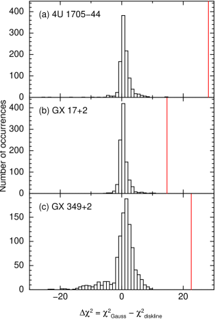
Figure 3.— Posterior predictive distributions for testing the likelihood that the diskline model gives the observed $\Delta\chi^{2}$ by chance for the BeppoSAX observations of (a) 4U 1705-44, (b) GX 17+2 and (c) GX 349+2 (observation 1 for each object). The distributions are histograms of $\Delta\chi^{2}=\chi^{2}(Gaussian)-\chi^{2}(diskline)$ from the 1000 simulations. The red, solid line indicates the $\Delta\chi^{2}$ measured from fitting the data. In none of the cases do any simulations show a $\Delta\chi^{2}$ as large as observed, indicating that the diskline model is strongly preferred.

We also perform another test of whether the diskline model fits better than a Gaussian by employing bootstrap resampling (see, e.g. Efron, 1979). This allows an estimation of the distribution in $\Delta\chi^{2}$ based on the distribution of the observed data. Bootstrap resampling consists of resampling the data with replacement. Thus, applying to spectra with $N$ events, we randomly select $N$ events from the spectrum, with replacement to create a new resampled spectrum. In this way some events get selected multiple times, where as others will not get selected at all. Doing this, we create 1000 resampled spectra from both the LECS and MECS detectors. We cannot do this for the PDS spectrum, as the pipeline produced spectrum is already background subtracted, and thus does not allow for a resampling of the detector events. However, as the region of interest (the Fe K line) is within the MECS detector, this is not an issue here. Thus, we resample the LECS and MECS spectra, but for the PDS we use the original data in the fit each time. For each set of resampled spectra, we fit both the diskline and Gaussian models (Model 2), and measure the $\Delta\chi^{2}$ between the fits. In Figure 4 we show the distribution of $\Delta\chi^{2}$ for the 1000 resamples for each three cases. As should be expected, the mean of the distribution is at approximately the $\Delta\chi^{2}$ of the data. Counting the fraction of samplings where $\Delta\chi^{2}>0$ (diskline better than a Gaussian) helps understand the significance of the diskline being a better fit than the Gaussian. For 4U 1705$-$44 we find 99.4% of resampled spectra have $\Delta\chi^{2}>0$, for GX 17+2 we find 99.8% and for GX 349+2 we find 100%. Again, strongly supporting that a diskline is the preferred model over a Gaussian.

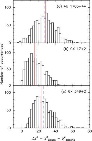
Figure 4.— Distributions of $\Delta\chi^{2}$ from bootstrap resampling of the BeppoSAX observations of (a) 4U 1705-44, (b) GX 17+2 and (c) GX 349+2 (again, observation 1 for each object). The distributions are histograms of $\Delta\chi^{2}=\chi^{2}(Gaussian)-\chi^{2}(diskline)$ from the 1000 resamplings. The red, solid line indicates the $\Delta\chi^{2}$ measured from fitting the data. The blue, dashed line indicates the mean $\Delta\chi^{2}$ from the simulations.

To determine whether the models used are appropriate, we perform a Kolmogorov-Smirnov (KS) test (e.g. Press et al., 1992). In the KS tests we determine the cumulative distribution function of the BeppoSAX/MECS spectrum as a function of energy, and compare this with the cumulative distribution function of the model. We do this for both the model with a Gaussian and the model with a diskline. We find that for all three cases for both the Gaussian and the diskline model that the KS probability = 1.0, indicating that both models are adequate descriptions of the data.

It is also important to consider whether we should have observed more asymmetric line profiles in these archival data. Clearly, the spectral resolution of RXTE/PCA is too low to be able to show line shapes similar to the Suzaku line profiles. For EXOSAT and BeppoSAX, where the spectral resolution (FWHM) at 6 keV is 0.6 and 0.5 keV respectively, the answer is not as immediately clear. The asymmetric Ser X-1 line as seen by Suzaku shows a narrow peak and broad wing which is not apparent in the EXOSAT and BeppoSAX data (see top left panel of Fig. 1 where the difference between the Suzaku and other line profiles can be seen). We have fit the EXOSAT and BeppoSAX spectra using a diskline with the parameters fixed to the Suzaku values (Cackett et al., 2010), except the line normalization which was variable in order to match the line strength. This intrinsically asymmetric line profile fits both spectra reasonably well ($\chi^{2}(dof)=214.9(185)$ for EXOSAT and $\chi^{2}(dof)=241.1(135)$ for BeppoSAX with Model 1), and there are no large residuals in the iron line region, though some residuals are present above 7 keV in the BeppoSAX data (we show the residuals in Figure 5). If the line parameters are allowed to be free parameters in the fit the parameters are not well constrained for EXOSAT (for instance the inclination tends to $90^{\circ}$). However, for BeppoSAX the $\chi^{2}$ improves slightly to $\chi^{2}(dof)=231.5(131)$, and apart from the normalization, the parameters remain close to the Suzaku values. For comparison, the best fitting line parameters from fitting the BeppoSAX data are: $E=6.97^{-0.04}$ keV, $\beta=-4.3\pm 0.5$, $R_{in}=6^{+1}$ GM/c², $i=28\pm 1$, norm = $(9.0\pm 0.7)\times 10^{-3}$. The difference between the Suzaku profile of Ser X-1 and the EXOSAT and BeppoSAX profiles is the most strikingly of the four sources, thus the fact that the Suzaku profile still fits the spectrum reasonably well demonstrates the significant smoothing by the lower resolution of those instruments, which may generally mask line asymmetry by blurring out the structure.

Figure 5.— Data/model for fits to the (a) EXOSAT  and (b) BeppoSAX data of Ser X-1. A diskline model was used to fit the Fe line, with all parameters except the normalization fixed at those determined from fits to Suzaku data in Cackett et al. (2010). There are no large residuals in the Fe line region, indicating the Suzaku diskline model fits well, though some residuals are apparent above 7 keV in the BeppoSAX data. Panel (c) is for the same data as (b) except that here all the line parameters are allowed to vary.

Furthermore, we perform additional simulations to see whether the $\Delta\chi^{2}$ value that we observe is what would be expected if the line profile during the BeppoSAX observations is the same as during the Suzaku observations. We therefore take the best-fitting BeppoSAX continuum (Model 2) and add a diskline with the same parameters as the best Suzaku fits (from Cackett et al., 2010), with only the normalization changed to match the EW seen in BeppoSAX observation. We perform 100 simulations, fitting the simulated spectra with both a Gaussian and diskline, and look at the distribution of $\Delta\chi^{2}$. For GX 349+2, we find that the median $\Delta\chi^{2}=31$, comparable to the $\Delta\chi^{2}=22.6$ that we observe from the real data. For GX 17+2, we find that the median $\Delta\chi^{2}=0.5$, much less significant than the $\Delta\chi^{2}=14.7$ from the real data. For 4U 1705-44. we find that the median $\Delta\chi^{2}=18.4$, a little less than the $\Delta\chi^{2}=28.2$ from the real data. This demonstrates that for GX 349+2 and 4U 1705$-$44 we see approximately the improvement in $\chi^{2}$ that we would expect based on the Suzaku line profiles, where as for GX 17+2 we see an even better improvement than expected.

4.2. Continuum model dependence

We fitted the data with two different continuum models. Model 1 contained a single temperature blackbody, disk-blackbody and a power-law (when needed), and Model 2 contained a single temperature blackbody, thermal Comptonization and a power-law (when needed). We generally find that Model 2 gives a better fit to the spectra than Model 1, and there is no clear dependence on source state or flux for this.

We consider how robust the Gaussian line widths are to the different continuum models. In Figure 6 we compare the line widths ($\sigma$) obtained when using both continuum models. We only compare observations where the two different models give equally good fits. We define equally good fits as the $\Delta\chi^{2}$ between the two models being less than 11.8. This is equivalent to 3$\sigma$ for the two additional degrees of freedom of Model 2 compared to Model 1. The exception to this is the Suzaku data where we find that only one observation has equally good fits, and so for illustrative purposes we show all the Suzaku observations.

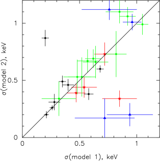
Figure 6.— A comparison of the Gaussian line widths measured when fitting the spectra with two different continuum models (model 1: diskbb + blackbody + power-law or model 2: bbody + comptt + power-law). Black circles represents data from Suzaku, red stars are from EXOSAT, blue triangles are from BeppoSAX, and green squares are from RXTE.

Generally, we find that there is a good agreement between the two models when equally good fits are compared. The biggest outliers that are not in agreement all have large uncertainties in the line widths. These are generally EXOSAT and BeppoSAX observations – the two missions with the lowest effective area, and also significantly lower spectral resolution than Suzaku. Given that most observations here have similar exposure times, it is clear these observations also have the lowest S/N.

It is interesting to note that the Suzaku and RXTE observations almost all give consistent results with differing models. While RXTE has the lowest spectral resolution, it has the highest effective area, whereas Suzaku has by the far the most superior spectral resolution. We can try and understand why there is a difference in the Gaussian line width with different models for EXOSAT and BeppoSAX by considering the line profiles seen by Suzaku. Firstly, in Figure 7 we show the Suzaku line profiles (when fit by a diskline model) for both continuum models. Clearly, the line profiles vary very little with the different continuum models, demonstrating that a robust line profile can be obtained with high spectral resolution and also good S/N. Note that the only Suzaku observation where there is a large difference in $\sigma$ is the first observation of 4U 1705$-$44, which is the observation with the lowest S/N of all the Suzaku observations, and one where in Cackett et al. (2010) we had to fix line parameters because they were poorly constrained.

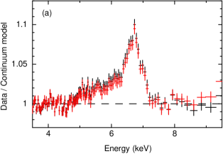
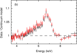
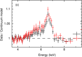
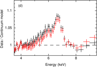
Figure 7.— A comparison of iron emission line profiles when fitting different continuum models to the Suzaku data. Panel (a) shows Serpens X-1, (b) GX 349+2 (observation 1), (c) GX 17+2 (observation 2), and (d) 4U 1705$-$44 (observation 2). In all panels, the spectra are from the combined front-illuminated XIS detectors. Black is when fitting with a diskbb component, while red is when the comptt component is used instead. Clearly, there is not a strong dependence on the choice of continuum model tested here.

The Suzaku  line profiles generally show a strong and quite narrow line peak, with a broader, weaker red wing. A single Gaussian does not fit the line profile well and, in fact, two Gaussians (one broad, one narrower) generally provide a better fit (Cackett et al., 2008). We also fit the Suzaku data with two Gaussians, and give the results in Table 11 (for observations where the addition of a second Gaussian improves the fit). Figure 8 illustrates how two Gaussians can fit the Suzaku line profile of GX 349+2.

Table 11Gaussian line parameters when fitting two Gaussians to Suzaku observations with an absorbed diskbb + bbody + power-law continuum model.

Source	Obs.	Gaussian				Gaussian				$\chi^{2}$ (dof)
		E (keV)	$\sigma$ (keV)	norm	EW (eV)	E (keV)	$\sigma$ (keV)	norm	EW (eV)
Serpens X$-$1	1	$6.40^{+0.16}$	$0.64\pm 0.04$	$(3.3\pm 0.4)\times 10^{-3}$	$53\pm 10$	$6.70\pm 0.01$	$0.14\pm 0.02$	$(1.1\pm 0.1)\times 10^{-3}$	$19\pm 5$	1464.6 (1104)
GX 349+2	1	$6.40^{+0.22}$	$0.72\pm 0.05$	$(1.4\pm 0.1)\times 10^{-2}$	$80\pm 10$	$6.79\pm 0.03$	$0.21\pm 0.03$	$(3.1\pm 0.5)\times 10^{-3}$	$20\pm 8$	1279.0 (1105)
GX 349+2	2	$6.40^{+0.34}$	$0.73\pm 0.07$	$(6.5\pm 1.1)\times 10^{-2}$	$48\pm 13$	$6.77\pm 0.02$	$0.24\pm 0.02$	$(4.0\pm 0.5)\times 10^{-3}$	$34\pm 10$	1253.5 (1105)
GX 17+2	2	$6.40^{+0.29}$	$0.50\pm 0.08$	$(4.9\pm 1.2)\times 10^{-2}$	$27\pm 11$	$6.64\pm 0.02$	$0.14\pm 0.03$	$(2.9\pm 0.6)\times 10^{-3}$	$17\pm 8$	650.9 (605)
4U 1705$-$44	2	$6.40^{+0.12}$	$0.72\pm 0.04$	$(3.3\pm 0.3)\times 10^{-3}$	$111\pm 19$	$6.70\pm 0.03$	$0.12\pm 0.03$	$(2.5\pm 0.6)\times 10^{-4}$	$9\pm 6$	1338.2 (1120)

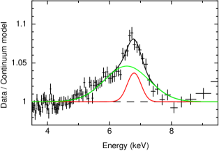
Figure 8.— A illustration that two Gaussians, one broad (green) and one narrower (red), can fit the line profile well in the Suzaku data of GX 349+2, observation 1. The combination of both Gaussians is shown as a black, solid line.

In the case of RXTE-type spectral resolution, the details of the line shape are blurred out by the line-spread function to a stage where the lines always appear Gaussian. The intermediate spectral resolution of EXOSAT and BeppoSAX, can show a hint of a red wing (see panel (c) in Fig. 1). However, whether a broad or narrow Gaussian fits the line profile best can depend on the underlying continuum model, though as we note above it is the observations with the largest uncertainty in line width that are the biggest outliers.

We therefore conclude that when different continuum models fit the data equally well, the line widths determined are generally consistent.

5. Discussion

We have studied spectra of four neutron star low-mass X-ray binaries (Ser X-1, GX 349+2, GX 17+2 and 4U 1705$-$44) from four different missions (EXOSAT, BeppoSAX, RXTE, Suzaku) in order to compare the iron line profiles. Our main result is that we find iron lines that show very similar line profiles between the four different missions examined (Fig. 1). Lines in the CCD spectra of Suzaku are not consistently broader than in the gas spectrometer data, demonstrating that the broad profiles are not a consequence of pile-up or other instrumental effects. Moreover, we found three BeppoSAX observations (one of GX 349+2, one of 4U 1705$-$44 and one of GX 17+2) that show evidence for asymmetry, with a relativistic disk-line model providing a better fit than a Gaussian. However, for data of average quality, the spectral resolution of the gas detectors ($\sim$0.5 keV for the best case looked at here, BeppoSAX/MECS) is not good enough to clearly show asymmetric profiles.

We also found that generally the continuum model choice leads to consistent iron line profiles when the models fit equally well. However, differences can arise and this is particularly a problem with the lower spectral resolution of gas spectrometers. However, with CCD spectral resolution and high S/N, we demonstrated that the line profiles can be robustly determined, regardless of the continuum model. This issue is more significant for neutron star LMXBs than black hole X-ray binaries due to the typically higher curvature and level of continuum degeneracy in the spectra of neutron star LMXBs.

The extensive simulations of Miller et al. (2010), the relativistic line profile detected in pile-up-free observations in 4U 1728$-$34 (Egron et al., 2011) in EPIC/pn “timing” mode, and the fact that the Suzaku line profiles do not change regardless of the extraction region used (Cackett et al., 2010) already comprise a large body of evidence suggesting that pile-up and instrumental effects are not the source of broad, asymmetric lines seen in neutron star LMXBs. Furthermore, our analysis of archival data presented here also shows that broad lines with comparable widths as the Suzaku data are seen in gas spectrometer data, where pile-up does not occur. In addition, three BeppoSAX observations also show evidence for asymmetric line profiles, with a relativistic line model providing a better fit than a Gaussian, and with the diskline parameters comparable with those observed by Suzaku.

It is also important to note that inferred upper limits on stellar radii are consistent with expectations from dense matter equations of state (Cackett et al., 2008). Furthermore, magnetic field estimates based on the inner disk radius measured from the Fe lines in two pulsars, SAXJ1808.4$-$3658 (Cackett et al., 2009; Papitto et al., 2009) and IGR J17480-2446 in the globular cluster Terzan 5 (Miller et al., 2011; Papitto et al., 2011), are consistent with the magnetic field estimates determined from timing methods. Thus, the measured inner disk radii are consistent with expectations.

The broadest iron lines in neutron star LMXBs, extend down to approximately 4.5 keV, i.e. approximately a 2 keV redshift. If due to Doppler broadening alone, such a shift in emission would indicate high velocities of the order $\sim$0.3c. This, of course, ignores any contribution from gravitational redshifts and Comptonization which will also broaden the line. Certainly, in highly ionized disks, Comptonization will be an important source of line broadening (see e.g. Ross & Fabian, 2007), but self-consistent reflection modeling which include those effects also indicate that the inner disk is close to the neutron star surface where relativistic blurring is strong (Reis et al., 2009; Cackett et al., 2010; D’Aì et al., 2010).

Reflection is further supported by the multiple observations of 4U 1705$-$44 considered by Lin et al. (2010). These authors show that the blackbody flux and iron line flux are strongly correlated in the soft states. This supports the hypothesis that the blackbody flux (possibly originating from the boundary layer) is the source of irradiating flux leading to reflection, at least in the soft states.

Thus far, studies of iron line variability between the states has been inconclusive. In the majority of work that has looked at this issue, there is no clear evidence of large changes between states (Iaria et al., 2009; Cackett et al., 2010; Lin et al., 2010; D’Aì et al., 2010). In the hard state of 4U 1705$-$44 there has been tentative evidence that the line may be narrower (Lin et al., 2010; D’Aì et al., 2010), though this may be an ionization effect (Reis et al., 2009). While a thorough study of line evolution with state is beyond the scope of this paper, it is interesting to point out that we do seem to see variability in the line profiles, at least in the case of GX 349+2.

The line profiles from the three BeppoSAX observations are shown in Figure 9. Detailed analysis of these BeppoSAX observations have previously been presented by Di Salvo et al. (2001) and Iaria et al. (2004), and both those papers carefully looked at variability in the Fe line. The variability we see is consistent with their work. Di Salvo et al. (2001) found a difference in the line EW when comparing spectra from flaring and non-flaring periods of the first BeppoSAX observation – the EW was larger in the non-flaring spectrum when there is a hard power-law tail extending up to 100 keV. Iaria et al. (2004) considered all the BeppoSAX observations, creating spectra based on the location in the color-color diagram. They found a very clear trend showing that the line EW decreases with increasing source luminosity. They note that the decrease in EW is due to both an increase in the continuum flux and a decrease in the line intensity. Interestingly, the spectra where the EW is strongest corresponds to the intervals where the hard power-law tail is strongest. Spectra from the flaring branch show the weakest line, and that is also where the hard power-law tail is not detected.

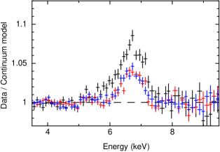
Figure 9.— A comparison of the line profiles from the three BeppoSAX observations of GX 349+2. Observation 1 (black) shows a stronger, broader line than observations 2 (red) or 3 (blue). See Table 7 for spectral parameters from these fits.

Cackett et al. (2010) and D’Aì et al. (2010) both discuss reflection in these neutron star LMXB systems, suggesting that, at least in the soft state, the irradiating source of hard X-ray flux is the boundary layer. However, in the first BeppoSAX observation of GX 349+2, there is also an additional hard power-law component at higher energies (Di Salvo et al., 2001). If this originates from a different region, for example a disk corona, then there could potentially be two sources of irradiation with different geometries leading to reflection.

6. Conclusions

To summarize our main findings:

• The iron line profiles seen in gas-based and CCD-based spectra are consistent. This demonstrates that the broad profiles are intrinsic to the lines and are not due to instrumental effects (such as pile-up).

• Several BeppoSAX observations of GX 349+2, GX 17+2 and 4U 1705$-$44 all show evidence for asymmetric line profiles. A relativistic diskline model fits better than a Gaussian line model as demonstrated by the posterior predictive p-value and bootstrapping methods.

• We also found that generally the continuum model choice leads to consistent iron line profiles when the models fit equally well. However, differences can arise and this is particularly a problem with the lower spectral resolution of gas spectrometers, but that line profiles determined by Suzaku are generally robust to the continuum choice.

References

- Arnaud (1996) Arnaud, K. A. 1996, in Astronomical Society of the Pacific Conference Series, Vol. 101, Astronomical Data Analysis Software and Systems V, ed. G. H. Jacoby & J. Barnes, 17
- Ballet (1999) Ballet, J. 1999, A&AS, 135, 371
- Barret (2001) Barret, D. 2001, Advances in Space Research, 28, 307
- Bhattacharyya & Strohmayer (2007) Bhattacharyya, S., & Strohmayer, T. E. 2007, ApJ, 664, L103
- Boella et al. (1997) Boella, G., Chiappetti, L., Conti, G., et al. 1997, A&AS, 122, 327
- Cackett et al. (2009) Cackett, E. M., Altamirano, D., Patruno, A., et al. 2009, ApJ, 694, L21
- Cackett et al. (2008) Cackett, E. M., Miller, J. M., Bhattacharyya, S., et al. 2008, ApJ, 674, 415
- Cackett et al. (2010) Cackett, E. M., Miller, J. M., Ballantyne, D. R., et al. 2010, ApJ, 720, 205
- D’Aì et al. (2009) D’Aì, A., Iaria, R., Di Salvo, T., Matt, G., & Robba, N. R. 2009, ApJ, 693, L1
- D’Aì et al. (2010) D’Aì, A., di Salvo, T., Ballantyne, D., et al. 2010, A&A, 516, A36
- Davis (2001) Davis, J. E. 2001, ApJ, 562, 575
- Di Salvo et al. (2001) Di Salvo, T., Robba, N. R., Iaria, R., et al. 2001, ApJ, 554, 49
- Di Salvo et al. (2000) Di Salvo, T., Stella, L., Robba, N. R., et al. 2000, ApJ, 544, L119
- Di Salvo et al. (2009) Di Salvo, T., D’Aí, A., Iaria, R., et al. 2009, MNRAS, 398, 2022
- Dickey & Lockman (1990) Dickey, J. M., & Lockman, F. J. 1990, ARA&A, 28, 215
- Efron (1979) Efron, B. 1979, Annals of Statistics, 7, 1
- Egron et al. (2011) Egron, E., di Salvo, T., Burderi, L., et al. 2011, A&A, 530, A99
- Fabian et al. (2000) Fabian, A. C., Iwasawa, K., Reynolds, C. S., & Young, A. J. 2000, PASP, 112, 1145
- Fabian et al. (1989) Fabian, A. C., Rees, M. J., Stella, L., & White, N. E. 1989, MNRAS, 238, 729
- Fabian et al. (2009) Fabian, A. C., Zoghbi, A., Ross, R. R., et al. 2009, Nature, 459, 540
- Farinelli et al. (2005) Farinelli, R., Frontera, F., Zdziarski, A. A., et al. 2005, A&A, 434, 25
- Fiocchi et al. (2007) Fiocchi, M., Bazzano, A., Ubertini, P., & Zdziarski, A. A. 2007, ApJ, 657, 448
- Gladstone et al. (2007) Gladstone, J., Done, C., & Gierliński, M. 2007, MNRAS, 378, 13
- Gottwald et al. (1995) Gottwald, M., Parmar, A. N., Reynolds, A. P., et al. 1995, A&AS, 109, 9
- Hirano et al. (1987) Hirano, T., Hayakawa, S., Nagase, F., Masai, K., & Mitsuda, K. 1987, PASJ, 39, 619
- Homan et al. (2002) Homan, J., van der Klis, M., Jonker, P. G., et al. 2002, ApJ, 568, 878
- Hurkett et al. (2008) Hurkett, C. P., et al. 2008, ApJ, 679, 587
- Iaria et al. (2009) Iaria, R., D’Aí, A., di Salvo, T., et al. 2009, A&A, 505, 1143
- Iaria et al. (2004) Iaria, R., Di Salvo, T., Robba, N. R., et al. 2004, ApJ, 600, 358
- Jahoda et al. (1996) Jahoda, K., Swank, J. H., Giles, A. B., et al. 1996, in Society of Photo-Optical Instrumentation Engineers (SPIE) Conference Series, Vol. 2808, Society of Photo-Optical Instrumentation Engineers (SPIE) Conference Series, ed. O. H. Siegmund & M. A. Gummin, 59–70
- Kuulkers & van der Klis (1995) Kuulkers, E., & van der Klis, M. 1995, in Annals of the New York Academy of Sciences, Vol. 759, Seventeeth Texas Symposium on Relativistic Astrophysics and Cosmology, ed. H. Böhringer, G. E. Morfill, & J. E. Trümper, 344
- Kuulkers et al. (1997) Kuulkers, E., van der Klis, M., Oosterbroek, T., van Paradijs, J., & Lewin, W. H. G. 1997, MNRAS, 287, 495
- Lin et al. (2007) Lin, D., Remillard, R. A., & Homan, J. 2007, ApJ, 667, 1073
- Lin et al. (2010) —. 2010, ApJ, 719, 1350
- Miller (2007) Miller, J. M. 2007, ARA&A, 45, 441
- Miller et al. (2011) Miller, J. M., Maitra, D., Cackett, E. M., Bhattacharyya, S., & Strohmayer, T. E. 2011, ApJ, 731, L7+
- Miller et al. (2010) Miller, J. M., D’Aì, A., Bautz, M. W., et al. 2010, ApJ, 724, 1441
- Mitsuda et al. (1989) Mitsuda, K., Inoue, H., Nakamura, N., & Tanaka, Y. 1989, PASJ, 41, 97
- Mitsuda et al. (2007) Mitsuda, K., et al. 2007, PASJ, 59, 1
- Muno et al. (2002) Muno, M. P., Remillard, R. A., & Chakrabarty, D. 2002, ApJ, 568, L35
- Ng et al. (2010) Ng, C., Díaz Trigo, M., Cadolle Bel, M., & Migliari, S. 2010, A&A, 522, A96
- Oosterbroek et al. (2001) Oosterbroek, T., Barret, D., Guainazzi, M., & Ford, E. C. 2001, A&A, 366, 138
- Papitto et al. (2011) Papitto, A., D’Aì, A., Motta, S., et al. 2011, A&A, 526, L3
- Papitto et al. (2009) Papitto, A., Di Salvo, T., D’Aì, A., et al. 2009, A&A, 493, L39
- Peacock et al. (1981) Peacock, A., Andresen, R. D., Manzo, G., et al. 1981, Space Sci. Rev., 30, 525
- Piraino et al. (2007) Piraino, S., Santangelo, A., di Salvo, T., et al. 2007, A&A, 471, L17
- Ponman et al. (1988) Ponman, T. J., Cooke, B. A., & Stella, L. 1988, MNRAS, 231, 999
- Press et al. (1992) Press, W. H., Teukolsky, S. A., Vetterling, W. T., & Flannery, B. P. 1992, Numerical recipes in FORTRAN. The art of scientific computing (Cambridge University Press)
- Protassov et al. (2002) Protassov, R., van Dyk, D. A., Connors, A., Kashyap, V. L., & Siemiginowska, A. 2002, ApJ, 571, 545
- Reis et al. (2009) Reis, R. C., Fabian, A. C., & Young, A. J. 2009, MNRAS, 399, L1
- Reynolds et al. (2009) Reynolds, C. S., Fabian, A. C., Brenneman, L. W., et al. 2009, MNRAS, 397, L21
- Reynolds & Nowak (2003) Reynolds, C. S., & Nowak, M. A. 2003, Phys. Rep., 377, 389
- Reynolds & Wilms (2000) Reynolds, C. S., & Wilms, J. 2000, ApJ, 533, 821
- Ross & Fabian (2007) Ross, R. R., & Fabian, A. C. 2007, MNRAS, 381, 1697
- Schulz et al. (1989) Schulz, N. S., Hasinger, G., & Truemper, J. 1989, A&A, 225, 48
- Seon & Min (2002) Seon, K.-I., & Min, K. W. 2002, A&A, 395, 141
- White et al. (1986) White, N. E., Peacock, A., Hasinger, G., et al. 1986, MNRAS, 218, 129
- White et al. (1985) White, N. E., Peacock, A., & Taylor, B. G. 1985, ApJ, 296, 475
- White et al. (1988) White, N. E., Stella, L., & Parmar, A. N. 1988, ApJ, 324, 363
- Wroblewski et al. (2008) Wroblewski, P., Guver, T., & Ozel, F. 2008, arXiv:0810.0007
- Zhang et al. (1998) Zhang, W., Strohmayer, T. E., & Swank, J. H. 1998, ApJ, 500, L167