The deconfinement phase transition in the Hamiltonian approach to Yang–Mills theory in Coulomb gauge

Abstract

The deconfinement phase transition of SU(2) Yang–Mills theory is investigated in the Hamiltonian approach in Coulomb gauge assuming a quasi-particle picture for the grand canonical gluon ensemble. The thermal equilibrium state is found by minimizing the free energy with respect to the quasi-gluon energy. Above the deconfinement phase transition the ghost form factor remains infrared divergent but its infrared exponent is approximately halved, while the gluon energy, being infrared divergent in the confined phase, becomes infrared finite in the deconfined phase. For the effective gluon mass we find a critical exponent of $0.37$. Using the lattice results for the gluon propagator to fix the scale, the deconfinement transition temperature is obtained in the range of $275$ to $290$ MeV.

I Introduction

Understanding the phase diagram of Quantum Chromodynamics (QCD) is one of the major challenges of particle physics. Running and upcoming, respectively, high-energy heavy-ion experiments at LHC, RHIC, SPS and FAIR, NICA and J-PARC call for a deeper understanding of hadronic matter under extreme conditions. The central issues are the equation of state of QCD and the nature of the phase transition from the confined hadronic phase with chiral symmetry spontaneously broken to the deconfined quark gluon plasma with chiral symmetry restored. The deconfinement phase transition is expected to be driven by the gluon dynamics, while the chiral phase transition, obviously, is due to strong interaction of the quarks, which, of course, is also mediated by the gluons. It is therefore by far non-trivial that both phase transitions occur at roughly the same temperature as observed on the lattice Karsch:2001cy .

In quenched QCD the deconfinement phase transition is related to the center of the gauge group. Center symmetry is realized in the low-temperature confined phase and spontaneously broken in the high-temperature deconfined phase Svetitsky:1982gs . When quarks are included center symmetry is explicitly broken and the deconfinement transition is expected to become a cross-over. The features of the chiral phase transition dominantly depend on the quark masses, which explicitly break chiral symmetry, but also on the strength of the chiral anomaly. Furthermore, lattice calculations also show that confinement is generated exclusively by the low-energy gluonic modes while also medium-energy gluon modes contribute to the order parameter of spontaneous breaking of chiral symmetry, the quark condensate Yamamoto:2009de .

Meanwhile by various theoretical studies evidence has been accumulated that the phase structure of hadronic matter is much richer than originally thought BraunMunzinger:2009zz . As the chemical potential or baryon density is increased one expects, on the basis of large-$N_{c}$ arguments, the existence of a “quarkyonic phase” where quarks and gluons are still confined but chiral symmetry is restored McLerran:2007qj . At even larger chemical potential the transition to color superconducting quark matter occurs with color-flavor locking Alford:2007xm . There are also speculations on the existence of a chiral critical endpoint for finite baryon density Fodor:2001pe .

Clearly the understanding of the phase structure and, in particular, the deconfinement phase transition requires, like the understanding of the confined phase itself, non-perturbative methods. A rigorous non-perturbative treatment of QCD is achieved on the lattice. The lattice method has been quite successful for quenched QCD but becomes extremely expensive when dynamical quarks are included and fails at large baryon densities due to the notorious fermion sign problem at non-vanishing chemical potential. Therefore, alternative non-perturbative methods which rely on the continuum formulation of QCD and thus do not suffer from the problem connected with the lattice treatment of fermions are very desirable. In recent years substantial progress has been made in first principle continuum QCD calculations, which rely on functional methods and do not suffer from the fermion problems of the lattice. Among these methods are Dyson–Schwinger equations (DSEs) in Landau Fischer:2006ub and Coulomb gauge Watson:2006yq , functional renormalization group (FRG) flow equations in Landau gauge Pawlowski:2005xe and Hamiltonian Coulomb gauge Leder:2010ji , and variational approaches to the Hamilton formulation of Yang–Mills theory in Coulomb gauge Schutte:1985sd ; *Szczepaniak:2001rg; Feuchter:2004mk . These various continuum methods have all their own advantages and drawbacks, and by combining them one expects to gain new insights into the non-perturbative regime of the theory. So far the deconfinement phase transition has been studied mainly in the FRG approach Pawlowski:2010ht ; Braun:2007bx or in the DSE approach Fischer:2009wc . The deconfinement temperature was extracted either directly from the Polyakov loop Braun:2007bx , which (in the absence of quarks) is the order parameter of confinement, or from the dual condensate Fischer:2009wc , which can be related to the Polyakov loop Gattringer:2006ci .

In this paper we study this transition in a variational approach to Hamiltonian Yang–Mills theory extending previous work Feuchter:2004mk to finite temperature.

In the variational approach at zero temperature the energy density is minimized using Gaussian type ansätze for the Yang–Mills vacuum wave functional Schutte:1985sd ; Szczepaniak:2001rg ; Feuchter:2004mk . So far, this approach has been mainly applied to study the infrared sector of Yang–Mills theory Schleifenbaum:2006bq ; Epple:2006hv , but was recently extended to full QCD Pak:2011wu . In the present paper we extend this approach to finite temperatures and study the deconfinement phase transition. For this purpose we will minimize the free energy after making an appropriate ansatz for the density matrix. Some initial investigations in this direction were undertaken in Ref. Reinhardt:2011hq , where, for simplicity, only the so-called subcritical solutions Epple:2007ut were considered, which do not produce confinement in the sense that they yield an infrared (IR) finite gluon energy and not a linearly rising (static) quark potential. As a consequence the deconfinement phase transition could not be studied. Furthermore, in Ref. Reinhardt:2011hq the projection of the grand canonical gluon ensemble onto zero color was considered and it was found that the effect of color projection is negligible. We will therefore ignore color projection in the present paper.

The organization of the paper is as follows: In Section II we briefly summarize the basic ingredients of the Hamiltonian approach to Yang–Mills theory in Coulomb gauge, which are needed for its extension to finite temperatures. In Section III we introduce the grand canonical ensemble of Yang–Mills theory. We define here the complete basis of the gluon Fock space as well as the density matrix following Ref. Reinhardt:2011hq . In Section IV we present the DSEs for the ghost and Coulomb propagator. In Section V we calculate the partition function, the entropy and the free energy. The variation of the free energy is carried out in Section VI and the renormalization of the resulting DSEs is given in Section VII. In Section VIII we present the results of an infrared analysis of the coupled DSEs and discuss the importance of the Coulomb term of the Yang–Mills Hamiltonian in Section IX. Finally, in Section XI we present the numerical solution of these DSEs and determine, in particular, the deconfinement transition temperature. A short summary and our conclusions are given in Section XII. The details of the IR analysis are presented in the Appendix.

II Hamiltonian approach to Yang–Mills theory in Coulomb gauge

Below we briefly summarize the basic ingredients of the Hamiltonian approach to Yang–Mills theory in Coulomb gauge Feuchter:2004mk needed for its extension to finite temperatures Reinhardt:2011hq .

To simplify the bookkeeping we will use the compact notation $A^{a_{1}}_{k_{1}}(\bm{\mathrm{x}}_{1})=A(1)$ for colored Lorentz vectors like the gauge potential and an analogous notation for colored Lorentz scalars like the ghost $C^{a_{1}}(\bm{\mathrm{x}}_{1})=C(1)$. A repeated label means summation over the discrete color (and Lorentz) indices along with integration over the $d$ spatial coordinates

$$A\cdot B=A(1)B(1)=\int\mathop{\mathrm{d}^{d}}\mkern-4.0mux\sum_{i=1}^{d}\sum_{a=1}^{N_{c}^{2}-1}A^{a}_{i}(\bm{\mathrm{x}})B^{a}_{i}(\bm{\mathrm{x}}).$$ (1)

We define in coordinate space

$$\delta(1,2)=\delta^{a_{1}a_{2}}t_{i_{1}i_{2}}(\bm{\mathrm{x}}_{1})\,\delta(\bm{\mathrm{x}}_{1}-\bm{\mathrm{x}}_{2}),$$ (2)

where

$$t_{ij}(\bm{\mathrm{x}})=\delta_{ij}-\frac{\partial_{i}\partial_{j}}{\partial^{2}}$$ (3)

is the transverse projector. Furthermore, indices will be suppressed when they can be easily restored from the context.

After resolving Gauss’s law in Coulomb gauge the Yang–Mills Hamiltonian Christ:1980ku reads in our notation

$$\begin{split}H={}&\frac{1}{2}\bigl{[}J^{-1}_{A}\Pi(1)J_{A}\Pi(1)+B(1)\,B(1)\bigr{]}\\ &+\frac{g^{2}}{2}J^{-1}_{A}\rho(1)J_{A}\,F_{A}(1,2)\rho(2)\\ \equiv{}&H_{K}+H_{B}+H_{\mathrm{C}},\end{split}$$ (4)

where $\Pi(1)=-\mathrm{i}\delta/\delta A(1)$ is the canonical momentum (electric field) operator, $B(1)$ is the non-abelian magnetic field

$$\bm{\mathrm{B}}^{a}=\bm{\mathrm{\nabla}}\bm{\times}\bm{\mathrm{A}}^{a}+\frac{g}{2}\>f^{abc}\bm{\mathrm{A}}^{b}\bm{\times}\bm{\mathrm{A}}^{c}\qquad(d=3),$$ (5)

$g$ is the coupling constant, and

$$\begin{split}J_{A}&=\operatorname{Det}G_{A}^{-1},\\ G^{-1}_{A}(1,2)&=\bigl{(}-\delta^{a_{1}a_{2}}\,{\partial^{2}_{\bm{\mathrm{x}}_{1}}}-g\,\hat{A}^{a_{1}a_{2}}_{i}(\bm{\mathrm{x}}_{1}){\partial_{i}^{\bm{\mathrm{x}}_{1}}}\bigr{)}\delta(\bm{\mathrm{x}}_{1}-\bm{\mathrm{x}}_{2})\end{split}$$ (6)

is the Faddeev–Popov determinant with $\hat{\bm{\mathrm{A}}}{}^{ab}=f^{acb}\bm{\mathrm{A}}^{c}$ being the gauge field in the adjoint representation of the gauge group SU($N_{c}$) with structure constants $f^{abc}$. Furthermore,

$$\begin{split}\rho(1)&\equiv\rho^{a_{1}}(\bm{\mathrm{x}}_{1})=R(1;2,3)A(2)\Pi(3),\\ R(1;2,3)&=f^{a_{1}a_{2}a_{3}}\,\delta_{i_{2}i_{3}}\,\delta(\bm{\mathrm{x}}_{1}-\bm{\mathrm{x}}_{2})\,\delta(\bm{\mathrm{x}}_{1}-\bm{\mathrm{x}}_{3})\end{split}$$ (7)

is the color charge density of the gluons and

$$F_{A}(1,2)\equiv F^{a_{1}a_{2}}_{A}(\bm{\mathrm{x}}_{1},\bm{\mathrm{x}}_{2})=G_{A}(1,3)\,G_{0}^{-1}(3,4)\,G_{A}(4,2)$$ (8)

is the so-called Coulomb kernel, with $G_{0}^{-1}$ being the bare inverse ghost operator, obtained by setting $A=0$ in Eq. (6). In the presence of matter fields with color charge density $\rho_{m}(1)$, the gluon charge $\rho(1)$ in the Coulomb term $H_{\mathrm{C}}$ [Eq. (4)] is replaced by the total charge $\rho(1)+\rho_{m}(1)$ and the vacuum expectation value of $F_{A}(1,2)$ acquires the meaning of the static non-abelian Coulomb potential.

The gauge fixed Hamiltonian Eq. (4) is highly non-local due to Coulomb kernel $F_{A}(1,2)$, Eq. (8), and due to the presence of the Faddeev–Popov determinant $J_{A}$, Eq. (6). In addition, the latter also occurs in the functional integration measure of matrix elements of operators ${\mathcal{O}}$ between Coulomb gauge wave functionals

$$\langle\psi_{1}|{\mathcal{O}}|\psi_{2}\rangle=\int DA\,J_{A}\,\psi^{*}_{1}[\bm{\mathrm{A}}]\,{\mathcal{O}}\,\psi_{2}[\bm{\mathrm{A}}],$$ (9)

where the integration runs over transverse field configurations. In practical calculations the elimination of unphysical degrees of freedom via gauge fixing is usually beneficial (and sometimes unavoidable), in spite of the increased complexity of the gauge-fixed Hamiltonian Eq. (4). The non-trivial Faddeev–Popov determinant reflects the intrinsically non-linear structure of the space of gauge orbits and dominates the IR behavior of the theory. Once Coulomb gauge is implemented, any functional of the (transverse) gauge field is a physical state.

III The grand canonical ensemble of Yang–Mills theory

We are interested in the behavior of Yang–Mills theory at finite temperatures. For this purpose we consider the grand canonical ensemble of Yang–Mills theory, which is defined in the Hamiltonian approach by the density matrix

$${\mathcal{D}}=\exp(-\beta H)$$ (10)

with $\beta=1/k_{\mathrm{B}}T$ being the inverse temperature measured in units of the Boltzmann constant $k_{\mathrm{B}}$. Formally, ${\mathcal{D}}$ [Eq. (10)] looks like the canonical ensemble since the chemical potential of the gluon vanishes. However, the thermal expectation values

$$\langle\!\langle{\mathcal{O}}\rangle\!\rangle=\frac{\operatorname{Tr}{\mathcal{D}}{\mathcal{O}}}{\operatorname{Tr}{\mathcal{D}}}=\frac{\sum_{k}\langle k\rvert{\mathcal{D}}{\mathcal{O}}\lvert k\rangle}{\sum_{k}\langle k\rvert{\mathcal{D}}\lvert k\rangle}$$ (11)

have to be taken over the whole Fock space, i.e. over states $\{\lvert k\rangle\}$ with an arbitrary number of gluons. Since $H$ is non-linear and non-local it is clear from the very beginning that we have to resort to approximations. We will use an analogous approximation scheme as in the zero-temperature case, see Ref. Feuchter:2004mk .

The trace in Eq. (11) can, in principle, be calculated in any complete basis $\{\lvert k\rangle\}$. Since we are mainly interested in $\langle\!\langle H\rangle\!\rangle$ we will choose a basis which is adapted to the structure of the Yang–Mills Hamiltonian. Following Refs. Feuchter:2004mk and Reinhardt:2011hq we choose the basis of the gluonic Fock space of the form

$$\langle A|k\rangle=J^{-1/2}_{A}\langle A|\tilde{k}\rangle,$$ (12)

where $\lvert\tilde{k}\rangle$ denotes a complete set of states of the Yang–Mills Fock space to be specified later. This ansatz removes the Faddeev–Popov determinant from the integration measure in Eq. (9). In this basis the thermal expectation value Eq. (11) reads

$$\langle\!\langle{\mathcal{O}}\rangle\!\rangle=\frac{\sum_{k}\langle\tilde{k}\rvert\tilde{{\mathcal{D}}}\tilde{{\mathcal{O}}}\lvert\tilde{k}\rangle}{\sum_{k}\langle\tilde{k}\rvert\tilde{{\mathcal{D}}}\lvert\tilde{k}\rangle}=\mathrel{\mathop{:}}\langle\tilde{{\mathcal{O}}}\rangle,$$ (13)

where we have introduced the abbreviation

$$\tilde{{\mathcal{O}}}=J^{1/2}_{A}{\mathcal{O}}J^{-1/2}_{A},$$ (14)

which yields for the density matrix Eq. (10)

$$\tilde{{\mathcal{D}}}=J^{1/2}_{A}{\mathcal{D}}J^{-1/2}_{A}=\mathrm{e}^{-\beta\tilde{H}}.$$ (15)

The transformed Yang–Mills Hamiltonian $\tilde{H}$ defined by Eq. (14) is obtained by replacing in the Yang–Mills Hamiltonian Eq. (4) the momentum operators $J^{-1}_{A}\Pi J_{A}\Pi$ by $\tilde{\Pi}^{\dagger}\tilde{\Pi}$, where

$$\tilde{\Pi}=J^{1/2}_{A}\Pi J^{-1/2}_{A}=\Pi+\frac{\mathrm{i}}{2}\frac{\delta\ln J_{A}}{\delta A}\,.$$ (16)

To work out the thermal averages it is convenient to go to momentum space

$$\begin{split}A(\bm{\mathrm{x}})&=\int\mathop{\mathrm{d}\mkern-7.0mu\mathchar 22\relax\mkern-1.0mu}\mkern-4.0mu{k}\>\mathrm{e}^{\mathrm{i}\bm{\mathrm{k}}\cdot\bm{\mathrm{x}}}\,A(\bm{\mathrm{k}}),\\ \Pi(\bm{\mathrm{x}})&=\int\mathop{\mathrm{d}\mkern-7.0mu\mathchar 22\relax\mkern-1.0mu}\mkern-4.0mu{k}\>\mathrm{e}^{-\mathrm{i}\bm{\mathrm{k}}\cdot\bm{\mathrm{x}}}\,\Pi(\bm{\mathrm{k}}),\end{split}$$ (17)

($\mathop{\mathrm{d}\mkern-7.0mu\mathchar 22\relax\mkern-1.0mu}\mkern-4.0mu{k}\equiv\mathop{\mathrm{d}^{d}}\mkern-4.0muk/(2\pi)^{d}$) where the Fourier components satisfy the commutation relation

$$\bigl{[}A(1),\Pi(2)\bigr{]}=\mathrm{i}\,\delta(1,2).$$ (18)

In the standard fashion we express the Fourier components in terms of creation and annihilation operators

$$A_{i}^{a}(\bm{\mathrm{k}}) =\frac{1}{\sqrt{2\omega(\bm{\mathrm{k}})}}\left(a_{i}^{a}(\bm{\mathrm{k}})+a_{i}^{a\dagger}(-\bm{\mathrm{k}})\right),$$ (19a)

$$\Pi_{i}^{a}(\bm{\mathrm{k}}) =\mathrm{i}\sqrt{\frac{\omega(\bm{\mathrm{k}})}{2}}\left(a_{i}^{a\dagger}(\bm{\mathrm{k}})-a_{i}^{a}(-\bm{\mathrm{k}})\right),$$ (19b)

which satisfy the usual commutation relations

$$\bigl{[}a_{i}^{a}(\bm{\mathrm{k}}),a_{j}^{b\dagger}(\bm{\mathrm{q}})\bigr{]}=\delta^{ab}t_{ij}(\bm{\mathrm{k}})(2\pi)^{d}\delta(\bm{\mathrm{k}}-\bm{\mathrm{q}}),$$ (20)

where $t_{ij}(\bm{\mathrm{k}})=\delta_{ij}-\hat{k}_{j}\hat{k}_{j}$, $\hat{\bm{\mathrm{k}}}=\bm{\mathrm{k}}/\lvert\bm{\mathrm{k}}\rvert$ is the transverse projector Eq. (3) in momentum space. Here $\omega(\bm{\mathrm{k}})$ is, so far, an arbitrary (positive definite) function of momenta. It enters the vacuum state $\lvert\tilde{0}\rangle$ defined by

$$a_{i}^{a}(\bm{\mathrm{k}})\lvert\tilde{0}\rangle=0,$$ (21)

which has the “coordinate” representation

$$\langle A|\tilde{0}\rangle={\mathcal{N}}\exp\left[-\tfrac{1}{2}A(1)\omega(1,2)A(2)\right],$$ (22)

where ${\mathcal{N}}$ is a normalization constant. The states

$$\lvert\tilde{0}\rangle,\quad a_{i}^{a\dagger}(\bm{\mathrm{k}})\lvert\tilde{0}\rangle,\quad a_{i}^{a\dagger}(\bm{\mathrm{k}})\,a_{j}^{b\dagger}(\bm{\mathrm{q}})\lvert\tilde{0}\rangle,\quad\dots$$ (23)

form a complete basis in the gluonic Fock space for any positive definite function $\omega(\bm{\mathrm{k}})$. Below we will use this basis to evaluate the thermal expectation values Eq. (13).

Because of the non-local structure of the Yang–Mills Hamiltonian [Eq. (4)], the density matrix Eq. (15) can only be treated in an approximate fashion. To make the actual calculation feasible we follow Ref. Reinhardt:2011hq and replace the full Yang–Mills Hamiltonian $\tilde{H}$ in the density operator $\tilde{{\mathcal{D}}}$ [Eq. (15)] by a single-particle operator

$$h=\int\mathop{\mathrm{d}\mkern-7.0mu\mathchar 22\relax\mkern-1.0mu}\mkern-4.0mu{k}\>a^{a\dagger}_{i}(\bm{\mathrm{k}})\,\Omega^{ab}(\bm{\mathrm{k}})\,a^{b}_{i}(\bm{\mathrm{k}}),$$ (24)

where $\Omega^{ab}(\bm{\mathrm{k}})$ will be later determined by minimizing the energy density, yielding

$$\tilde{{\mathcal{D}}}=\exp(-\beta h).$$ (25)

By global color and rotational invariance, $\Omega^{ab}(\bm{\mathrm{k}})$ is color-diagonal and independent of color, $\Omega^{ab}(\bm{\mathrm{k}})=\delta^{ab}\Omega(\bm{\mathrm{k}})$, and furthermore depends only on $\lvert\bm{\mathrm{k}}\rvert$. The same is true for the kernel $\omega$ in the vacuum wave functional Eq. (22). Since the transformed density matrix $\tilde{{\mathcal{D}}}$ [Eq. (25)] is the exponential of a single-particle operator Wick’s theorem applies to the thermal averages Eq. (13), whose temperature dependence is exclusively given by the finite-temperature Bose occupation numbers $n(\bm{\mathrm{k}})$, defined (in momentum space) by

$$\begin{split}\langle a_{i}^{a\dagger}(\bm{\mathrm{k}})\,a_{j}^{b}(\bm{\mathrm{q}})\rangle&=\delta^{ab}t_{ij}(\bm{\mathrm{k}})(2\pi)^{d}\delta(\bm{\mathrm{k}}-\bm{\mathrm{q}})\,n(\bm{\mathrm{k}}),\\ \qquad n(\bm{\mathrm{k}})&=\bigl{[}\exp\bigl{(}\beta\Omega(\bm{\mathrm{k}})\bigr{)}-1\bigr{]}^{-1}.\end{split}$$ (26)

From Eqs. (19a) and (19b) one finds for the gluon propagator

$$D(1,2)\mathrel{\mathop{:}}=\langle A(1)A(2)\rangle,\qquad D(\bm{\mathrm{k}})=\frac{1+2n(\bm{\mathrm{k}})}{2\omega(\bm{\mathrm{k}})},$$ (27)

for the momentum propagator

$$K(1,2)\mathrel{\mathop{:}}=\langle\Pi(1)\Pi(2)\rangle,\qquad K(\bm{\mathrm{k}})=\frac{1+2n(\bm{\mathrm{k}})}{2}\>\omega(\bm{\mathrm{k}}),$$ (28)

and for the “mixed” propagator

$$\langle A(1)\Pi(2)\rangle=\frac{\mathrm{i}}{2}\>\delta(1,2),$$ (29)

the latter being independent of the temperature.

IV Ghost and Coulomb propagator

We will resort to the same approximation used in Ref. Feuchter:2004mk in the $T=0$ case, i.e. calculating the energy up to two loops. To this order the following representation of the Faddeev–Popov determinant holds Reinhardt:2004mm

$$J_{A}=\exp\left[-A(1)\chi(1,2)A(2)\right],$$ (30)

where

$$\chi(1,2)=-\frac{1}{2}\left<\frac{\delta^{2}\ln J_{A}}{\delta A(1)\delta A(2)}\right>$$ (31)

is the so-called curvature, which, in fact, represents the ghost loop (see below). Strictly speaking this representation was derived only for $T=0$. However, the proof given in Ref. Reinhardt:2004mm can be straightforwardly extended to finite temperatures provided the density matrix $\tilde{{\mathcal{D}}}$ is the exponential of a single particle operator, so that Wick’s theorem holds for the thermal averages $\langle\tilde{{\mathcal{O}}}\rangle$ [Eq. (13)]. This is the case for the density matrix Eq. (25). With the inverse Faddeev–Popov operator $G_{A}$ [see Eq. (6)] the curvature Eq. (31) can be expressed as

$$\chi(1,2)=\frac{1}{2}\left<\widetilde{\Gamma}_{0}(1;3,4)\,G_{A}(3^{\prime},3)\,\widetilde{\Gamma}_{0}(2;4^{\prime},3^{\prime})\,G_{A}(4,4^{\prime})\right>,$$ (32)

where

$$\widetilde{\Gamma}_{0}(1;2,3)=\frac{\delta G_{A}^{-1}(2,3)}{\delta A(1)}$$ (33)

is the bare ghost-gluon-vertex. Defining the ghost propagator by

$$G=\langle G_{A}\rangle$$ (34)

and the full ghost-gluon vertex $\widetilde{\Gamma}$ by

$$\langle G_{A}\widetilde{\Gamma}_{0}G_{A}\rangle=G\widetilde{\Gamma}G,$$ (35)

the ghost loop Eq. (32) becomes

$$\chi(1,2)=\frac{1}{2}\widetilde{\Gamma}_{0}(1;3,4)\,G(3^{\prime},3)\,\widetilde{\Gamma}(2;4^{\prime},3^{\prime})\,G(4,4^{\prime}).$$ (36)

Furthermore, the ghost propagator $G$ satisfies the Dyson equation Feuchter:2004mk

$$G=G_{0}+G_{0}\Sigma G,$$ (37)

where

$$G^{ab}_{0}(\bm{\mathrm{x}},\bm{\mathrm{y}})=\bigl{[}(-\partial^{2})^{-1}\bigr{]}_{\bm{\mathrm{x}},\bm{\mathrm{y}}}^{ab}$$ (38)

is the free ghost propagator and

$$\Sigma(1,2)=\widetilde{\Gamma}_{0}(3;1,4)\,G(4,4^{\prime})\,D(3,3^{\prime})\,\widetilde{\Gamma}(3^{\prime};4^{\prime},2)$$ (39)

is the ghost self-energy. As shown in Landau gauge Taylor:1971ff the ghost-gluon vertex is not renormalized; this applies also in Coulomb gauge, see Ref. Schleifenbaum:2006bq . At zero temperature the full ghost-gluon vertex $\widetilde{\Gamma}$ can be, to good approximation, replaced by the bare one $\widetilde{\Gamma}_{0}$ Campagnari:2011bk . We assume that this approximation works also at finite temperatures. Assuming a bare ghost-gluon vertex and expressing the ghost propagator Eq. (34) in momentum space by the ghost form factor

$$G^{ab}(\bm{\mathrm{k}})=\delta^{ab}\frac{d(\bm{\mathrm{k}})}{g\,\bm{\mathrm{k}}^{2}}$$ (40)

the curvature Eq. (36) becomes in momentum space

$$\chi(\bm{\mathrm{k}})=\frac{N_{c}}{2(d-1)}\int\mathop{\mathrm{d}\mkern-7.0mu\mathchar 22\relax\mkern-1.0mu}\mkern-4.0mu{q}\bigl{[}1-(\hat{\bm{\mathrm{k}}}\cdot\hat{\bm{\mathrm{q}}})^{2}\bigr{]}\frac{d(\bm{\mathrm{k}}-\bm{\mathrm{q}})\,d(\bm{\mathrm{q}})}{(\bm{\mathrm{k}}-\bm{\mathrm{q}})^{2}},$$ (41)

and the ghost form factor $d(\bm{\mathrm{k}})$ satisfies the following DSE

$$d^{-1}(\bm{\mathrm{k}})=\frac{1}{g}-I_{d}(\bm{\mathrm{k}}),$$ (42)

where

$$I_{d}(\bm{\mathrm{k}})=N_{c}\int\mathop{\mathrm{d}\mkern-7.0mu\mathchar 22\relax\mkern-1.0mu}\mkern-4.0mu{q}\bigl{[}1-(\hat{\bm{\mathrm{k}}}\cdot\hat{\bm{\mathrm{q}}})^{2}\bigr{]}\frac{d(\bm{\mathrm{k}}-\bm{\mathrm{q}})}{(\bm{\mathrm{k}}-\bm{\mathrm{q}})^{2}}\frac{1+2n(\bm{\mathrm{q}})}{2\omega(\bm{\mathrm{q}})}\,.$$ (43)

As at zero temperature we express the Coulomb propagator

$$F(1,2)=\langle F_{A}(1,2)\rangle$$ (44)

by means of the Coulomb form factor $f(\bm{\mathrm{k}})$ defined in momentum space by

$$g^{2}F^{ab}(\bm{\mathrm{k}})=g^{2}\delta^{ab}\,G(\bm{\mathrm{k}})f(\bm{\mathrm{k}})\,\bm{\mathrm{k}}^{2}G(\bm{\mathrm{k}})=\delta^{ab}\frac{d(\bm{\mathrm{k}})^{2}}{\bm{\mathrm{k}}^{2}}\,f(\bm{\mathrm{k}}).$$ (45)

Using the operator identity

$$F_{A}=\frac{\partial}{\partial g}(gG_{A})$$ (46)

and, proceeding as in the zero-temperature case (see e.g. Ref. Feuchter:2004mk ), neglecting the $g$-dependence of the density matrix one finds the relation

$$f(\bm{\mathrm{k}})=-g^{2}\frac{\partial}{\partial g}d^{-1}(\bm{\mathrm{k}})$$ (47)

from which one finds with Eq. (42) the following integral equation

$$f(\bm{\mathrm{k}}) =1+I_{f}(\bm{\mathrm{k}})$$ (48)

$$I_{f}(\bm{\mathrm{k}}) =N_{c}\int\mathop{\mathrm{d}\mkern-7.0mu\mathchar 22\relax\mkern-1.0mu}\mkern-4.0mu{q}\bigl{[}1-(\hat{\bm{\mathrm{k}}}\cdot\hat{\bm{\mathrm{q}}})^{2}\bigr{]}\begin{aligned} &\frac{d(\bm{\mathrm{k}}-\bm{\mathrm{q}})^{2}\,f(\bm{\mathrm{k}}-\bm{\mathrm{q}})}{(\bm{\mathrm{k}}-\bm{\mathrm{q}})^{2}}\\ &\times\frac{1+2n(\bm{\mathrm{q}})}{2\omega(\bm{\mathrm{q}})}\,.\end{aligned}$$ (49)

This equation is formally the same as at zero temperature except that the gluon propagator is replaced by its finite-temperature counterpart, Eq. (27).

V The free energy

At vanishing chemical potential the thermodynamic potential of the grand canonical ensemble is given by the free energy

$${\mathcal{F}}=\langle\tilde{H}\rangle-T{\mathcal{S}},$$ (50)

where ${\mathcal{S}}$ is the entropy, which is defined by

$${\mathcal{S}}=-k_{\mathrm{B}}\operatorname{Tr}\left[\frac{\tilde{{\mathcal{D}}}}{\tilde{Z}}\>\ln\frac{\tilde{{\mathcal{D}}}}{\tilde{Z}}\right],$$ (51)

where

$$\tilde{Z}=\operatorname{Tr}\tilde{{\mathcal{D}}}$$ (52)

is the partition function of the grand canonical ensemble with $\tilde{{\mathcal{D}}}$ defined by Eq. (15). By straightforward algebraic manipulation the entropy Eq. (51) can be converted to

$${\mathcal{S}}=k_{\mathrm{B}}\biggl{(}\ln\tilde{Z}-\beta\frac{\partial\ln\tilde{Z}}{\partial\beta}\biggr{)}.$$ (53)

In principle, we could calculate the free energy from the partition function, $\tilde{Z}=\exp(-\beta{\mathcal{F}})$. For the exact density matrix Eq. (15) this would yield the same result as Eq. (50). However, in the present case, where we have replaced the full density matrix Eq. (15) by the one of a system of independent quasi-particles, Eq. (25), it is mandatory to evaluate ${\mathcal{F}}$ from Eq. (50) in order to capture the essential correlations between the gluons. Besides, the density matrix $\tilde{{\mathcal{D}}}$ Eq. (25) has so far not been determined.

The partition function of the density matrix $\tilde{{\mathcal{D}}}$ [Eq. (25)] is calculated in the standard fashion yielding

$$\tilde{Z}=\exp\left[(d-1)(N^{2}_{c}-1)V\int\mathop{\mathrm{d}\mkern-7.0mu\mathchar 22\relax\mkern-1.0mu}\mkern-4.0mu{k}\>\ln\bigl{(}1+n(\bm{\mathrm{k}})\bigr{)}\right],$$ (54)

where $d-1=t_{ii}(\bm{\mathrm{k}})$ is the number of independent polarization directions in $d$ spatial dimensions and $N^{2}_{c}-1$ is the number of color degrees of freedom of the gauge bosons. With Eq. (54) we find from Eq. (53) for the entropy density $s[n]$ per degree of freedom of the gauge bosons, defined by

$${\mathcal{S}}=(d-1)(N^{2}_{c}-1)V\frac{1}{(2\pi)^{d}}s[n],$$ (55)

the expression

$$s[n]=(2\pi)^{d}k_{\mathrm{B}}\int\mathop{\mathrm{d}\mkern-7.0mu\mathchar 22\relax\mkern-1.0mu}\mkern-4.0mu{k}\left[\beta n(\bm{\mathrm{k}})\Omega(\bm{\mathrm{k}})+\ln\bigl{(}1+n(\bm{\mathrm{k}})\bigr{)}\right],$$ (56)

where $\Omega(\bm{\mathrm{k}})$ is the variational kernel in the density matrix [Eq. (24)]. To obtain the free energy from Eq. (50) we have still to calculate the energy $\langle\tilde{H}\rangle$, which is done below.

In the evaluation of the expectation value of the Yang–Mills Hamiltonian Eq. (4) we use the same approximation as in the $T=0$ case keeping only terms up to two loops in the energy Feuchter:2004mk . The magnetic energy is straightforwardly evaluated using Wick’s theorem. One finds

$$\langle\tilde{H}_{B}\rangle=\frac{(d-1)(N_{c}^{2}-1)}{4}\,V\int\mathop{\mathrm{d}\mkern-7.0mu\mathchar 22\relax\mkern-1.0mu}\mkern-4.0mu{p}\>\frac{\bm{\mathrm{p}}^{2}}{\omega(\bm{\mathrm{p}})}[1+2n(\bm{\mathrm{p}})]\\ +\frac{g^{2}N_{c}(N_{c}^{2}-1)}{16}\,V\int\mathop{\mathrm{d}\mkern-7.0mu\mathchar 22\relax\mkern-1.0mu}\mkern-4.0mu{p}\mathop{\mathrm{d}\mkern-7.0mu\mathchar 22\relax\mkern-1.0mu}\mkern-4.0mu{q}\>\frac{d(d-3)+3-(\hat{\bm{\mathrm{p}}}\cdot\hat{\bm{\mathrm{q}}})^{2}}{\omega(\bm{\mathrm{p}})\omega(\bm{\mathrm{q}})}\\ \times\bigl{[}1+2n(\bm{\mathrm{p}})\bigr{]}\bigl{[}1+2n(\bm{\mathrm{q}})\bigr{]}.$$ (57)

The evaluation of the kinetic energy and the Coulomb energy is somewhat more involved. With the representation Eq. (30) we obtain from Eq. (16)

$$\tilde{\Pi}(1)=\Pi(1)-\mathrm{i}\,\chi(1,2)A(2).$$ (58)

For the expectation value of the two momentum operators entering the kinetic and Coulomb terms one finds by using Eqs. (58) and (27)–(29)

$$\langle\tilde{\Pi}^{\dagger}(1)\tilde{\Pi}(2)\rangle=K(1,2)-\chi(1,2)+\chi(1,1^{\prime})D(1^{\prime},2^{\prime})\chi(2^{\prime},2).$$ (59)

Contracting the external indices one obtains from this expression immediately the expectation value of the kinetic term

$$\langle\tilde{H}_{K}\rangle=\frac{1}{2}\langle\tilde{\Pi}^{\dagger}(1)\tilde{\Pi}(1)\rangle\\ =\frac{1}{2}\left[K(1,1)-\chi(1,1)+\chi(1,2)D(2,3)\chi(3,1)\right]\\ =\frac{(d-1)(N_{c}^{2}-1)}{2}\,V\int\mathop{\mathrm{d}\mkern-7.0mu\mathchar 22\relax\mkern-1.0mu}\mkern-4.0mu{q}\bigl{[}K(\bm{\mathrm{q}})-\chi(\bm{\mathrm{q}})\\ +\chi^{2}(\bm{\mathrm{q}})D(\bm{\mathrm{q}})\bigr{]}.$$ (60)

This expression is not obviously positive definite (as it should be); however, it is not difficult to show that this is indeed the case. Using Eqs. (27) and (28) and separating the zero- and finite-temperature terms, Eq. (60) can be written as

$$\langle\tilde{H}_{K}\rangle=\frac{(d-1)(N_{c}^{2}-1)}{2}\,V\int\mathop{\mathrm{d}\mkern-7.0mu\mathchar 22\relax\mkern-1.0mu}\mkern-4.0mu{q}\Biggl{\{}\frac{\bigl{[}\omega(\bm{\mathrm{q}})-\chi(\bm{\mathrm{q}})\bigr{]}^{2}}{2\omega(\bm{\mathrm{q}})}\\ +n(\bm{\mathrm{q}})\>\frac{\omega^{2}(\bm{\mathrm{q}})+\chi^{2}(\bm{\mathrm{q}})}{\omega(\bm{\mathrm{q}})}\Biggr{\}},$$ (61)

from which it is seen that $\langle\tilde{H}_{K}\rangle$ is indeed positive definite.

Restricting ourselves to including up to two (overlapping) loops in the energy allows us to replace the Coulomb kernel $F_{A}(1,2)$ in $\tilde{H}_{\mathrm{C}}$ by its expectation value Eq. (44), resulting in the approximation

$$\langle\rho(1)F_{A}(1,2)\rho(2)\rangle\\ \simeq\langle F_{A}(1,2)\rangle R(1;3,4)R(2;5,6)\langle A(3)\tilde{\Pi}^{\dagger}(4)A(5)\tilde{\Pi}(6)\rangle\\ =F(1,2)R(1;3,4)R(2;5,6)\Bigl{[}\langle A(3)A(5)\rangle\langle\tilde{\Pi}^{\dagger}(4)\tilde{\Pi}(6)\rangle\\ +\langle A(3)\tilde{\Pi}(6)\rangle\langle\tilde{\Pi}^{\dagger}(4)A(5)\rangle\Bigr{]}.$$ (62)

The remaining expectation values can be straightforwardly carried out using Eqs. (58) and (59). Then we find for the Coulomb term

$$\langle\tilde{H}_{\mathrm{C}}\rangle=\frac{g^{2}}{2}F(1,2)R(1;3,4)R(2;5,6)\\ \times\Bigl{\{}D(3,5)\bigl{[}K(4,6)-\chi(4,6)+\chi(4,4^{\prime})D(4^{\prime},6^{\prime})\chi(6^{\prime},6)\bigr{]}\\ +\Bigl{[}\tfrac{1}{2}\>\delta(3,6)-D(3,3^{\prime})\chi(3^{\prime},6)\Bigr{]}\\ \times\Bigl{[}\tfrac{1}{2}\>\delta(4,5)-\chi(4,4^{\prime})D(4^{\prime},5)\Bigr{]}\Bigr{\}}.$$ (63)

As noticed in Ref. Reinhardt:2011hq , with the replacement

$$F^{ab}_{A}(\bm{\mathrm{x}},\bm{\mathrm{y}})\to\delta^{ab}$$ (64)

the Coulomb Hamiltonian $H_{\mathrm{C}}$ [Eq. (4)] becomes

$$H_{\mathrm{C}}\to\frac{g^{2}}{2}J^{-1}_{A}Q^{a}J_{A}Q^{a}=\frac{g^{2}}{2}Q^{a}Q^{a},$$ (65)

where

$$Q^{a}=\int\mathop{\mathrm{d}^{d}}\mkern-4.0mux\>\rho^{a}(\bm{\mathrm{x}})$$ (66)

is the total color charge and we have used

$$[Q^{a},J_{A}]=0.$$ (67)

The last relation holds since the Faddeev–Popov determinant $J_{A}$ is invariant under global color rotations, which are generated by $Q^{a}$. This is also explicitly seen by using the representation Eq. (30). In a colorless universe

$$\langle\!\langle Q^{a}Q^{a}\rangle\!\rangle\equiv\langle\tilde{Q}^{a}\tilde{Q}^{a}\rangle=\langle{Q}^{a}{Q}^{a}\rangle=0$$ (68)

holds. To ensure that this condition (68) is respected by $\langle H_{\mathrm{C}}\rangle$ in Ref. Reinhardt:2011hq the Coulomb kernel $\frac{g^{2}}{2}F^{ab}_{A}(\bm{\mathrm{x}},\bm{\mathrm{y}})$ was replaced by

$$\frac{g^{2}}{2}F^{ab}_{A}(\bm{\mathrm{x}},\bm{\mathrm{y}})-\delta^{ab}.$$ (69)

Furthermore, in Ref. Reinhardt:2011hq the Yang–Mills grand canonical ensemble was projected onto zero total color. It was found in there that the effects of both color projection and of the replacement Eq. (69) is negligible. Therefore in the following we will ignore the projection on zero color states [as well as the replacement Eq. (69)].

Rewriting the above given thermal average of the Hamiltonian, Eqs. (57), (60) and (63), in momentum space one finds for the energy density per degree of freedom $e[n,\omega]$ defined by

$$\begin{split}\langle\tilde{H}\rangle&=(d-1)(N^{2}_{c}-1)\frac{V}{(2\pi)^{d}}\>e[n,\omega],\\ e[n,\omega]&\equiv e_{K}+e_{B}+e_{\mathrm{C}}\end{split}$$ (70)

the following expressions

$$e_{K}={} \frac{(2\pi)^{d}}{2}\int\mathop{\mathrm{d}\mkern-7.0mu\mathchar 22\relax\mkern-1.0mu}\mkern-4.0mu{q}\left[K(\bm{\mathrm{q}})-\chi(\bm{\mathrm{q}})+\chi^{2}(\bm{\mathrm{q}})D(\bm{\mathrm{q}})\right],$$ (71a)

$$e_{B}={} \frac{(2\pi)^{d}}{2}\,\int\mathop{\mathrm{d}\mkern-7.0mu\mathchar 22\relax\mkern-1.0mu}\mkern-4.0mu{q}\>\bm{\mathrm{q}}^{2}\,D(\bm{\mathrm{q}})+\frac{g^{2}(2\pi)^{d}N_{c}(d-1)^{2}}{4d}\,\int\mathop{\mathrm{d}\mkern-7.0mu\mathchar 22\relax\mkern-1.0mu}\mkern-4.0mu{p}\mathop{\mathrm{d}\mkern-7.0mu\mathchar 22\relax\mkern-1.0mu}\mkern-4.0mu{q}\>D(\bm{\mathrm{p}})D(\bm{\mathrm{q}}),$$ (71b)

$$e_{\mathrm{C}}={} \frac{g^{2}N_{c}}{4(d-1)}(2\pi)^{d}\int\mathop{\mathrm{d}\mkern-7.0mu\mathchar 22\relax\mkern-1.0mu}\mkern-4.0mu{p}\mathop{\mathrm{d}\mkern-7.0mu\mathchar 22\relax\mkern-1.0mu}\mkern-4.0mu{q}\bigl{[}d-2+(\hat{\bm{\mathrm{p}}}\cdot\hat{\bm{\mathrm{q}}})^{2}\bigr{]}F(\bm{\mathrm{p}}+\bm{\mathrm{q}})\Bigl{\{}D(\bm{\mathrm{p}})K(\bm{\mathrm{q}})+D(\bm{\mathrm{q}})K(\bm{\mathrm{p}})+D(\bm{\mathrm{p}})D(\bm{\mathrm{q}})\bigl{[}\chi(\bm{\mathrm{p}})-\chi(\bm{\mathrm{q}})\bigr{]}^{2}$$

$$+\bigl{[}D(\bm{\mathrm{p}})-D(\bm{\mathrm{q}})\bigr{]}\bigl{[}\chi(\bm{\mathrm{p}})-\chi(\bm{\mathrm{q}})\bigr{]}-\tfrac{1}{2}\Bigr{\}},$$ (71c)

where $F(\bm{\mathrm{k}})$ is the Coulomb propagator defined by Eqs. (44) and (45).

VI The finite-temperature variational principle

The kernel $\Omega(\bm{\mathrm{k}})$ defining the density matrix $\tilde{{\mathcal{D}}}$ [see Eqs. (24) and (25)] is so far completely arbitrary. We will now determine it by the finite-temperature variational principle. At fixed temperature and volume and arbitrary particle number the thermodynamic potential to be minimized is the grand canonical potential, which in the present case coincides with the free energy since the chemical potential of the gluons vanishes. Therefore we minimize the free energy or its density

$$f[n,\omega]=e[n,\omega]-Ts[n],$$ (72)

where $e[n,\omega]$ is the energy density [Eq. (70)] and $s[n]$ is the entropy density [Eq. (56)]. Instead of varying the free energy density with respect to $\Omega(\bm{\mathrm{k}})$ it is more convenient to take the variation with respect to the occupation numbers $n(\bm{\mathrm{k}})$ [Eq. (26)], which is equivalent since $n(\bm{\mathrm{k}})$ is a monotonic function of $\Omega(\bm{\mathrm{k}})$. From Eq. (56) we find for the variation of the entropy

$$\frac{\delta s[n]}{\delta n(\bm{\mathrm{k}})}=\frac{1}{T}\>\Omega(\bm{\mathrm{k}}).$$ (73)

Therefore stationarity of the free energy density, $\delta f/\delta n=0$, requires

$$\Omega(\bm{\mathrm{k}})=\frac{\delta e[n,\omega]}{\delta n(\bm{\mathrm{k}})}\,,$$ (74)

which, in the spirit of Landau’s Fermi liquid theory, identifies $\Omega(\bm{\mathrm{k}})$ as the quasi-gluon energy. Of course, this result could have been anticipated from the form of the finite-temperature Bose occupation numbers, Eq. (26).

So far the kernel $\omega(\bm{\mathrm{k}})$, which defines the vacuum wave functional [Eq. (22)] and thus our basis of the Fock space, is completely arbitrary and we could use any positive definite kernel and the corresponding gluon basis to calculate the thermodynamic averages. As long as we include the complete set of states and keep the full canonical density operator the thermodynamical averages are independent of $\omega(\bm{\mathrm{k}})$. Thus, in principle, the free energy should not depend on $\omega(\bm{\mathrm{k}})$. However, due to the truncation of the full Hamiltonian in the density operator $\tilde{{\mathcal{D}}}$ [Eq. (15)] to a single particle one [Eq. (25)] the actual choice of the basis, i.e. of $\omega(\bm{\mathrm{k}})$, does matter and the optimal choice of $\omega(\bm{\mathrm{k}})$ is obtained by extremizing the free energy

$$\frac{\delta f[n,\omega]}{\delta\omega(\bm{\mathrm{k}})}=0.$$ (75)

For the evaluation of $\delta e[n,\omega]/\delta\omega(\bm{\mathrm{k}})$ we skip the implicit $\omega(\bm{\mathrm{k}})$ dependence of $\chi(\bm{\mathrm{k}})$ and $F(\bm{\mathrm{k}})$, since their inclusion would give rise to higher-order loops. Ignoring this implicit $\omega(\bm{\mathrm{k}})$ dependence the energy density depends on $n(\bm{\mathrm{k}})$ and $\omega(\bm{\mathrm{k}})$ only through the gluon field and momentum propagators, $D$ [Eq. (27)] and $K$ [Eq. (28)], i.e.

$$e[n,\omega]=e\left[D[n,\omega],K[n,\omega]\right].$$ (76)

Using the chain rule and the explicit form of the propagators [Eqs. (27) and (28)] we obtain

$$\frac{\delta e}{\delta n(\bm{\mathrm{k}})} =\frac{1}{\omega(\bm{\mathrm{k}})}\frac{\delta e}{\delta D(\bm{\mathrm{k}})}+\omega(\bm{\mathrm{k}})\frac{\delta e}{\delta K(\bm{\mathrm{k}})},$$ (77)

$$\frac{\delta e}{\delta\omega(\bm{\mathrm{k}})} =\frac{1+2n(\bm{\mathrm{k}})}{2}\left[\frac{\delta e}{\delta D(\bm{\mathrm{k}})}-\omega^{2}(\bm{\mathrm{k}})\frac{\delta e}{\delta K(\bm{\mathrm{k}})}\right].$$ (78)

Since the entropy density $s[n]$ [Eq. (56)] does not explicitly depend on $\omega(\bm{\mathrm{k}})$ the condition Eq. (75) reduces to

$$\delta e[n,\omega]/\delta\omega(\bm{\mathrm{k}})=0\,,$$ (79)

which in view of Eq. (78) leads to the condition

$$\frac{\delta e}{\delta D(\bm{\mathrm{k}})}=\omega^{2}(\bm{\mathrm{k}})\frac{\delta e}{\delta K(\bm{\mathrm{k}})}\,.$$ (80)

For $T=0$, which implies $n(\bm{\mathrm{k}})=0$, this equation reduces to the gap equation obtained in Ref. Feuchter:2004mk . Inserting the gap equation (80) into Eq. (77) we find from Eq. (74)

$$\Omega(\bm{\mathrm{k}})=2\omega(\bm{\mathrm{k}})\frac{\delta e}{\delta K(\bm{\mathrm{k}})}\,.$$ (81)

With the explicit expressions for the energy density given in Eq. (71) we obtain

$$\frac{\Omega(\bm{\mathrm{k}})}{\omega(\bm{\mathrm{k}})}=1+I_{\Omega}(\bm{\mathrm{k}})\,,$$ (82)

where

$$I_{\Omega}(\bm{\mathrm{k}})=\frac{g^{2}\,N_{c}}{2(d-1)}\int\mathop{\mathrm{d}\mkern-7.0mu\mathchar 22\relax\mkern-1.0mu}\mkern-4.0mu{q}\bigl{[}d-2+(\hat{\bm{\mathrm{k}}}\cdot\hat{\bm{\mathrm{q}}})^{2}\bigr{]}F(\bm{\mathrm{k}}-\bm{\mathrm{q}})\>\frac{1+2n(\bm{\mathrm{q}})}{{\omega(\bm{\mathrm{q}})}}.$$ (83)

Using the explicit expressions for the energy density [Eq. (71)], the gap equation can finally be expressed as

$$\omega^{2}(\bm{\mathrm{k}})=\bm{\mathrm{k}}^{2}+\chi^{2}(\bm{\mathrm{k}})+I^{0}_{\omega}[n]+I_{\omega}[n](\bm{\mathrm{k}}),$$ (84)

where

$$I^{0}_{\omega}[n]=\frac{g^{2}N_{c}(d-1)^{2}}{2d}\int\mathop{\mathrm{d}\mkern-7.0mu\mathchar 22\relax\mkern-1.0mu}\mkern-4.0mu{q}\>\frac{1+2n(\bm{\mathrm{q}})}{{\omega(\bm{\mathrm{q}})}}$$ (85)

is the tadpole term stemming from the non-abelian part of the magnetic energy, and

$$I_{\omega}[n](\bm{\mathrm{k}})=\frac{g^{2}N_{c}}{2(d-1)}\int\mathop{\mathrm{d}\mkern-7.0mu\mathchar 22\relax\mkern-1.0mu}\mkern-4.0mu{q}\bigl{[}d-2+(\hat{\bm{\mathrm{k}}}\cdot\hat{\bm{\mathrm{q}}})^{2}\bigr{]}\frac{F(\bm{\mathrm{k}}-\bm{\mathrm{q}})}{\omega(\bm{\mathrm{q}})}\\ \times\Bigl{\{}\bigl{(}1+2n(\bm{\mathrm{q}})\bigr{)}\bigl{[}\omega^{2}(\bm{\mathrm{q}})-\omega^{2}(\bm{\mathrm{k}})+\bigl{(}\chi(\bm{\mathrm{q}})-\chi(\bm{\mathrm{k}})\bigr{)}^{2}\bigr{]}\\ -2\omega(\bm{\mathrm{q}})\bigl{(}\chi(\bm{\mathrm{q}})-\chi(\bm{\mathrm{k}})\bigr{)}\Bigr{\}}$$ (86)

is the contribution of the Coulomb Hamiltonian. These loop integrals are ultraviolet (UV) divergent and require regularization and eventually renormalization of the gap equation. Fortunately the temperature dependence of these loop integrals (which is due to the finite-temperature occupation numbers $n(\bm{\mathrm{k}})$) does not give rise to additional UV singularities. Therefore the zero-temperature counterterms are, in principle, sufficient to eliminate the UV singularities. However, special care is required to separate the temperature dependence from the UV-singular terms, which will be done in the next section.

VII Renormalization

At large momenta $\lvert\bm{\mathrm{k}}\rvert\gg k_{\mathrm{B}}T$ the temperature should become irrelevant. Consequently, the finite-temperature solutions $\omega(\bm{\mathrm{k}})$, $d(\bm{\mathrm{k}})$, $\chi(\bm{\mathrm{k}})$ should possess the same UV behavior as in the zero-temperature case. Indeed, the finite-temperature contributions to the loop integrals (the terms proportional to the occupation number $n(\bm{\mathrm{k}})$) are all ultraviolet finite. This is because for $\lvert\bm{\mathrm{k}}\rvert\to\infty$ we have $\Omega(\bm{\mathrm{k}})\sim\omega(\bm{\mathrm{k}})\sim k$ and thus the finite-temperature occupation numbers

$$n(\bm{\mathrm{q}}\to\infty)\sim\mathrm{e}^{-\beta\Omega(\bm{\mathrm{q}}\to\infty)}\sim\mathrm{e}^{-\beta q}$$ (87)

cut off the large momenta. Therefore, the renormalization can be done independent of the temperature subtracting only zero-temperature counterterms.

For the renormalization we follow Ref. Feuchter:2004mk and separate the various degrees of UV divergences of the loop integrals of the gap equation by writing Eq. (86) as

$$I_{\omega}[n](\bm{\mathrm{k}})=I_{\omega}^{(2)}(\bm{\mathrm{k}},T)+2\chi(\bm{\mathrm{k}})I_{\omega}^{(1)}(\bm{\mathrm{k}},T)+\bar{I}_{\omega}[n](\bm{\mathrm{k}}),$$ (88)

where the integrals

$$I_{\omega}^{(l)}(\bm{\mathrm{k}},T)=\frac{g^{2}N_{c}}{2(d-1)}\int\mathop{\mathrm{d}\mkern-7.0mu\mathchar 22\relax\mkern-1.0mu}\mkern-4.0mu{q}\bigl{[}d-2+(\hat{\bm{\mathrm{k}}}\cdot\hat{\bm{\mathrm{q}}})^{2}\bigr{]}\frac{F(\bm{\mathrm{k}}-\bm{\mathrm{q}})}{\omega(\bm{\mathrm{q}})}\\ \times\Bigl{[}\bigl{(}\omega(\bm{\mathrm{q}})-\chi(\bm{\mathrm{q}})\bigr{)}^{l}-\bigl{(}\omega(\bm{\mathrm{k}})-\chi(\bm{\mathrm{k}})\bigr{)}^{l}\Bigr{]}$$ (89)

are linearly (for $l=1$) and quadratically (for $l=2$) UV divergent, while the finite-temperature contribution

$$\bar{I}_{\omega}[n](\bm{\mathrm{k}})=\frac{g^{2}N_{c}}{d-1}\int\mathop{\mathrm{d}\mkern-7.0mu\mathchar 22\relax\mkern-1.0mu}\mkern-4.0mu{q}\bigl{[}d-2+(\hat{\bm{\mathrm{k}}}\cdot\hat{\bm{\mathrm{q}}})^{2}\bigr{]}\frac{F(\bm{\mathrm{k}}-\bm{\mathrm{q}})}{\omega(\bm{\mathrm{q}})}\\ \times n(\bm{\mathrm{q}})\Bigl{[}\omega^{2}(\bm{\mathrm{q}})-\omega^{2}(\bm{\mathrm{k}})+\bigl{(}\chi(\bm{\mathrm{q}})-\chi(\bm{\mathrm{k}})\bigr{)}^{2}\Bigr{]}$$ (90)

is UV convergent due to Eq. (87). Analogously we write for the tadpole Eq. (85)

$$I_{\omega}^{0}[n]=I_{\omega}^{0}+\bar{I}_{\omega}^{0}[n],\qquad I_{\omega}^{0}\equiv I_{\omega}^{0}[n=0].$$ (91)

The loop integrals $I_{\omega}^{(l)}(\bm{\mathrm{k}},T)$ and $I_{\omega}^{0}$ are defined as in the zero-temperature case, Ref. Feuchter:2004mk . However, their entries $\omega(\bm{\mathrm{k}})$, $d(\bm{\mathrm{k}})$, and $\chi(\bm{\mathrm{k}})$ are temperature dependent. These integrals contain all UV divergences, while the finite-temperature modifications $\bar{I}_{\omega}[n](\bm{\mathrm{k}})$ and $\bar{I}_{\omega}^{0}[n]$ are UV finite. Therefore, the renormalization can be carried out, in principle, in the same way as in the zero-temperature case, Ref. Reinhardt:2007wh . However, due to the implicit temperature dependence of $\omega(\bm{\mathrm{k}}),d(\bm{\mathrm{k}}),\chi(\bm{\mathrm{k}})$ we have to be careful not to introduce finite-temperature effects by the renormalization. Following the renormalization procedure given in Ref. Reinhardt:2007wh for $T=0$ and subtracting only zero-temperature terms one arrives at the renormalized gap equation

$$\omega^{2}(\bm{\mathrm{k}})=\bm{\mathrm{k}}^{2}+\overline{\chi}^{2}(\bm{\mathrm{k}})+\Delta I_{\omega}^{(2)}(\bm{\mathrm{k}})+\Delta I_{\omega}^{0}+\bar{I}_{\omega}^{0}[n]+c_{0}\\ +2\overline{\chi}(\bm{\mathrm{k}})\bigl{[}\Delta I_{\omega}^{(1)}(\bm{\mathrm{k}})+c_{1}\bigr{]}+\bar{I}_{\omega}[n](\bm{\mathrm{k}}),$$ (92)

where

$$\overline{\chi}(\bm{\mathrm{k}}) =\chi(\bm{\mathrm{k}})-\chi(\mu_{\chi})|_{T=0}$$

$$\Delta I_{\omega}^{(l)}(\bm{\mathrm{k}}) =I_{\omega}^{(l)}(\bm{\mathrm{k}})-I_{\omega\rvert_{T=0}}^{(l)}(0)$$

$$\Delta I_{\omega}^{0} =I_{\omega}^{0}-I_{\omega\rvert_{T=0}}^{0}$$ (93)

and $c_{0}$, $c_{1}$ are finite renormalization constants surviving from energy counterterms Epple:2007ut

$$\Delta H=\frac{1}{2}\,C_{0}\,A(1)A(1)+\mathrm{i}C_{1}A(1)\Pi(1).$$ (94)

$c_{0}$ and $c_{1}$ are the finite parts of the divergent constants $C_{0}$ and $C_{1}$, respectively, i.e. $C_{i}=C_{i}^{\mathit{div}}+c_{i}$. Furthermore, $\mu_{\chi}$ is an arbitrary scale arising from the renormalization of the Faddeev–Popov determinant Epple:2007ut . The subscript $T=0$ in Eq. (VII) means that the corresponding quantities have to be taken with the zero-temperature self-consistent solution. The choice of these finite renormalization parameters will be discussed in Sect. X.

The renormalized ghost DSE is obtained from Eq. (42) with a subtraction at an arbitrary scale $\mu_{d}$ at $T=0$

$$\begin{split}d^{-1}(\bm{\mathrm{k}})&=d^{-1}(\mu_{d})-\Delta I_{d}(\bm{\mathrm{k}}),\\ \Delta I_{d}(\bm{\mathrm{k}})&=I_{d}(\bm{\mathrm{k}})-I_{d}(\mu_{d})\big{\rvert}_{T=0}\,.\end{split}$$ (95)

The Gribov-Zwanziger confinement scenario requires the horizon condition

$$d^{-1}(k=0)\big{\rvert}_{T=0}=0,$$ (96)

to be satisfied at $T=0$. This condition can be explicitly built in the renormalized ghost DSE (95) by choosing the renormalization constant $d(\mu_{d})$ such that

$$d^{-1}(\mu_{d})=\Delta I_{d}(k=0)\big{\rvert}_{T=0}=I_{d}(0)\big{\rvert}_{T=0}-I_{d}(\mu_{d})\big{\rvert}_{T=0}\,,$$ (97)

which can be fulfilled for arbitrary renormalization scale $\mu_{d}$. Inserting this value into Eq. (95) we obtain

$$d^{-1}(\bm{\mathrm{k}})=-\bigl{(}I_{d}(\bm{\mathrm{k}})-I_{d}(0)\big{\rvert}_{T=0}\bigr{)},$$ (98)

which is nothing but the renormalized ghost DSE (95) with the renormalization scale fixed at $\mu_{d}=0$ [and the horizon condition Eq. (96) built in]. This shows that implementing the horizon condition automatically puts the renormalization scale in Eq. (95) to $\mu_{d}=0$. Solutions of the coupled DSEs and gap equation satisfying the horizon condition (96) are called “critical” and those with $d^{-1}(0)>0$ subcritical Epple:2007ut .

The renormalized DSE for the Coulomb form factor $f(\bm{\mathrm{k}})$ [Eq. (45)] is analogously obtained by subtracting Eq. (48) once at $T=0$ and an arbitrary renormalization scale $\mu_{f}$, yielding

$$\begin{split}f(\bm{\mathrm{k}})&=f(\mu_{f})+\Delta I_{f}(\bm{\mathrm{k}}),\\ \Delta I_{f}(\bm{\mathrm{k}})&=I_{f}(\bm{\mathrm{k}})-I_{f}(\mu_{f})\bigr{\rvert}_{T=0}\,.\end{split}$$ (99)

In principle, the renormalization scale $\mu_{f}$ of the Coulomb form factor can be independently chosen from that of the ghost $\mu_{d}$. However, since $f(\bm{\mathrm{k}})$ and $d(\bm{\mathrm{k}})$ are tightly related by Eq. (47) for consistency one should choose $\mu_{f}=\mu_{d}$.

Within our approach the finite-temperature Yang–Mills theory is now determined by the following set of coupled equations: The Eq. (82) for the quasi-gluon energy $\Omega(\bm{\mathrm{k}})$, the gap equation (92) for $\omega(\bm{\mathrm{k}})$, the DSE (95) for the ghost form factor $d(\bm{\mathrm{k}})$ and the DSE (99) for the Coulomb form factor $f(\bm{\mathrm{k}})$.

A comment is here in order: In principle, we would get only two equations from the finite-temperature variational principle, one equation for $\Omega(\bm{\mathrm{k}})$ and one for $\omega(\bm{\mathrm{k}})$. However, in the process of evaluating $\langle\tilde{H}\rangle$ we have introduced, for convenience, additional propagators (ghost and Coulomb propagator), which we did not explicitly express as functionals of $\omega(\bm{\mathrm{k}})$ (and $\Omega(\bm{\mathrm{k}})$). Instead of that we derived DSEs for these quantities, which all contain loop integrals. In taking the variation of the energy $\langle\tilde{H}\rangle$ with respect to $\omega(\bm{\mathrm{k}})$ and $\Omega(\bm{\mathrm{k}})$ the implicit $\omega(\bm{\mathrm{k}})$ — and $\Omega(\bm{\mathrm{k}})$ — dependence of these propagators is ignored since it would give rise to two-loop terms in the equations of motion, see Ref. Campagnari:2010wc for more details.

VIII Infrared analysis

Before presenting the numerical solutions of the coupled Eqs. (82), (92), (98) and (99), we investigate their infrared behavior. At zero temperature the infrared analysis was carried out in Refs. Feuchter:2004mk ; Schleifenbaum:2006bq . At arbitrary finite temperature the infrared analysis of the DSEs cannot be done in the usual way. This is because the finite-temperature occupation numbers $n(\bm{\mathrm{k}})$ [Eq. (26)] depend exponentially on the gluon quasi-energy $\Omega(\bm{\mathrm{k}})$. The infrared analysis can, however, be carried out in the high-temperature limit where the occupation numbers become

$$n(\bm{\mathrm{k}})\overset{T\to\infty}{\sim}\frac{k_{\mathrm{B}}T}{\Omega(\bm{\mathrm{k}})}\,.$$ (100)

This limit is sufficient to exhibit the infrared behavior of the propagators in the deconfined phase. With the representation Eq. (100) the infrared analysis of the coupled Dyson–Schwinger equations can essentially be carried out as at $T=0$.

In general, the IR analysis can be carried out in two ways: i) using the angular approximation Feuchter:2004mk replacing kernels $K(\bm{\mathrm{k}}-\bm{\mathrm{q}})$ depending on the difference between the external momentum $\bm{\mathrm{k}}$ and the loop momentum $\bm{\mathrm{q}}$ by

$$K(\bm{\mathrm{k}}-\bm{\mathrm{q}})\to K(k)\,\Theta(k-q)+K(q)\,\Theta(q-k),$$ (101)

with $k=\lvert\bm{\mathrm{k}}\rvert$, $q=\lvert\bm{\mathrm{q}}\rvert$. Although being approximative, this method has the advantage that IR power law ansätze for the propagators are indeed restricted to the IR regime. ii) Without using the angular approximation the IR power law ansätze have to be used in the loop integrals for the whole momentum range Lerche:2002ep ; Schleifenbaum:2006bq . This method is, in principle, exact in the IR (up to the omission of possible logarithms) but has the disadvantage that the UV behavior of these integrals is usually changed by the IR power law ansätze and UV-finite loop integrals may turn into UV-divergent ones. Fortunately both methods yield very similar results as we will explicitly demonstrate in the Appendix.

For the infrared analysis we assume the following power law ansätze

$$\omega(\bm{\mathrm{k}}\to 0)\sim\frac{A}{k^{\alpha}}\,,\qquad d(\bm{\mathrm{k}}\to 0)\sim\frac{B}{k^{\beta}}.$$ (102)

For $T=0$ the infrared analysis with and without angular approximation was carried out in Refs. Feuchter:2004mk and Schleifenbaum:2006bq , respectively. Assuming the horizon condition [Eq. (96)] and a bare ghost-gluon vertex one finds from the ghost DSE (42) in $d$ spatial dimensions in both cases the sum rule

$$\alpha=2\beta+2-d.$$ (103)

Including also the gap equation the infrared exponents are fixed and one finds, abandoning the angular approximation, in $d=3$ spatial dimensions two solutions Schleifenbaum:2006bq

$$\beta\simeq 0.8,\qquad\beta=1.$$ (104)

(In the angular approximation only the second solution is obtained.) Both exponents are also found in the numerical solutions, and were originally obtained in Ref. Feuchter:2004mk ($\beta\simeq 0.8$) and in Ref. Epple:2006hv ($\beta=1$). In $d=2$ spatial dimensions one finds a single solution with $\beta=1/2$ in the angular approximation and $\beta=0.4$ when the angular approximation is abandoned, while the numerical solution Feuchter:2007mq yields $\beta\simeq 0.44$.

For high temperatures using the approximation Eq. (100) the infrared analysis is carried out in the Appendix. From the ghost DSE one finds the same sum rule Eq. (103) as in the zero-temperature case. Including also the gap equation one obtains in $d=3$ at high temperatures a solution with the infrared exponent of the ghost form factor

$$\beta=1/2\,$$ (105)

both with and without the angular approximation. With this value for $\beta$ one finds from the infrared analysis of the DSE for the Coulomb form factor $f(\bm{\mathrm{k}}\to 0)\sim 1/k^{\lambda}$ the infrared exponent $\lambda\approx 1$ which together with $\beta=1/2$ for the ghost form factor leads to a linearly rising Coulomb potential $F(\bm{\mathrm{k}}\to 0)\sim 1/k^{4}$, as is also found in the lattice calculation Nakagawa:2006fk . The infrared exponents obtained in the infrared analysis are confirmed by the numerical calculations, as we will see in Section XI.

IX Neglect of the Coulomb term

We are mainly interested in the description of the deconfinement phase transition. If the Gribov confinement scenario is realized in Coulomb gauge, this transition should manifest itself in a change of the infrared behavior of the various propagators, in particular in that of the ghost form factor $d(\bm{\mathrm{k}})$ and the gluon energy $\omega(\bm{\mathrm{k}})$ and $\Omega(\bm{\mathrm{k}})$, respectively. In the (renormalized) gap equation (92) the contributions from the Coulomb term are infrared sub-leading ($\Delta I^{(l)}(k=0)=0$) even for infrared finite $\omega(\bm{\mathrm{k}})$. Furthermore, the ghost DSE (42) does not receive contributions from the Coulomb term. Therefore, for a first qualitative description of the deconfinement phase transition the Coulomb term should be negligible. With the neglect of the Coulomb term, the gap equation (92), reduces to

$$\omega^{2}(\bm{\mathrm{k}})=\bm{\mathrm{k}}^{2}+\overline{\chi}^{2}(\bm{\mathrm{k}})+\Delta I_{\omega}^{0}+\bar{I}^{0}_{\omega}[n]+c_{0}+2c_{1}\overline{\chi}(\bm{\mathrm{k}}),$$ (106)

while the ghost DSE (98) remains unchanged. At $T=0$ both $\Delta I^{0}_{\omega}$ [Eq. (VII)] and $\bar{I}^{0}_{\omega}[n]$ [Eq. (91)] vanish and the gap equation (106) reduces to

$$\omega^{2}(\bm{\mathrm{k}})=\bm{\mathrm{k}}^{2}+\overline{\chi}^{2}(\bm{\mathrm{k}})+2c_{1}\overline{\chi}(\bm{\mathrm{k}})+c_{0}\,.$$ (107)

Figure 1 shows the result of the numerical solution of the ghost DSE and the full gap equation (92) at $T=0$ and the corresponding solutions of the gap equation (107) with the Coulomb term neglected for $c_{0}=c_{1}=0$.

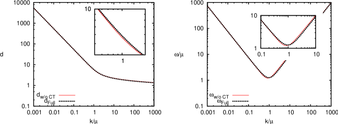
Figure 1: The ghost form factor (left panel) and the gluon energy (right panel) at $T=0$ with and without the Coulomb term.

As is seen, there are only small deviations in the mid-momentum regime, while both solutions agree in the ultraviolet and, in particular, in the infrared. Furthermore, in a quasi-particle description of the gluon sector (underlying the present approach) the neglect of the Coulomb term is conceptually advantageous (and expected to give a better description) as long as two particle correlations are neglected. The reason is the following: The Coulomb term gives rise to the UV-singular quasi-gluon self-energy, $\Delta\Omega(\bm{\mathrm{k}})=\omega(\bm{\mathrm{k}})I_{\Omega}(\bm{\mathrm{k}})$, see Eq. (82), which is diagrammatically illustrated in Fig. 2a. In a two-(quasi-)gluon state these divergent self-energy contributions are precisely canceled by the divergent contribution from the Coulomb interaction to the two-gluon energy, shown in Fig. 2b.

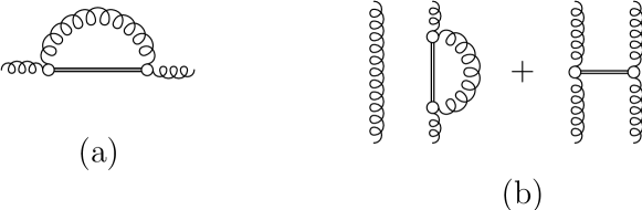
Figure 2: Contributions of the Coulomb term to (a) the gluon self-energy and (b) the two-gluon energy. A wavy line represents the gluon propagator, the double line stands for the Coulomb kernel.

Therefore it does not make sense to keep the Coulomb term in the quasi-gluon energy as long as the two-body correlations are not taken into account. We will therefore neglect the Coulomb term in the following. Then the loop integral in Eq. (82) has to be discarded so that

$$\Omega(\bm{\mathrm{k}})=\omega(\bm{\mathrm{k}}).$$ (108)

Furthermore, $\Delta I^{0}_{\omega}$ [Eq. (VII)] represents the change of the tadpole due to the change of the self-consistent solution $\omega(\bm{\mathrm{k}})$ at finite temperature (relative to the zero-temperature case) but does not contain the change of the tadpole due to the explicit temperature dependence of the gluon propagator via the finite-temperature occupation numbers. Therefore, we expect $\Delta I^{0}_{\omega}$ to be small and we will neglect it. Then the finite-temperature gap equation (106) reduces to

$$\omega^{2}(\bm{\mathrm{k}})=\bm{\mathrm{k}}^{2}+\overline{\chi}^{2}(\bm{\mathrm{k}})+\bar{I}_{\omega}^{0}[n]+2c_{1}\,\overline{\chi}(\bm{\mathrm{k}})+c_{0}\,.$$ (109)

Here only $\bar{I}^{0}_{\omega}[n]$ (the temperature-dependent part of the tadpole, see Eq. (91)) is explicitly temperature dependent, while the curvature $\chi(\bm{\mathrm{k}})$ depends only implicitly on the temperature via the ghost form factor. However, as we will see in Sect. XI, it is this temperature dependence of the ghost which triggers the deconfinement phase transition.

X Choice of renormalization constants

Let us now discuss the choice of the finite renormalization parameters. Since the renormalization can be completely accomplished by renormalizing the theory at zero temperature, the remaining finite-temperature renormalization constants $c_{0}$, $c_{1}$ should be also fixed at $T=0$ and then kept fixed independent of the temperature. To fix these constants we notice that the $T=0$ solutions are IR divergent with $\omega(k)\sim\chi(k)\sim 1/k^{\alpha}$, $\alpha=0.8$, $1$, see Sect. VIII. For such solutions the gap equation (107) reduces in the IR with Eq. (102) to

$$\omega(k)-\overline{\chi}(k)=c_{1}+\frac{c_{0}}{2A}\>k^{\alpha}+\dots$$ (110)

The constant $c_{1}$ obviously determines the infrared limit of $\omega(\bm{\mathrm{k}})-\overline{\chi}(\bm{\mathrm{k}})$, and $c_{1}=0$ is required in order that the ’t Hooft loop obeys an area law, Ref. Reinhardt:2007wh . This value is also favored by the variational principle (of minimal energy), Ref. Reinhardt:2007wh . Furthermore, recent lattice investigations of the Yang–Mills vacuum wave functional in $d=2$ spatial dimensions show that for this value of $c_{1}$ the wave functional Eq. (22) yields statistical weights for abelian plane-wave configurations which are in very good agreement with the ones of the exact vacuum wave functional Greensite:2011pj . We will therefore put $c_{1}=0$.

As is seen from Eq. (110) the renormalization constant $c_{0}$ is IR subleading compared to $c_{1}$ and influences the mid-momentum regime, which is however expected to affect the deconfinement phase transition. Fortunately in the present variational approach $c_{0}$ needs not to be treated as a free parameter but can be determined by minimizing the energy density. First notice that with $c_{1}=0$ the IR behavior of the $T=0$ gap equation (110) reduces to

$$\omega(k)-\overline{\chi}(k)=\frac{c_{0}}{2A}\>k^{\alpha}+\dots$$ (111)

Furthermore, with Eq. (30), which is correct to the two-loop order (in the energy) considered in the present paper, our vacuum wave functional defined by Eqs. (12) and (22) reads

$$\langle A|0\rangle=\mathcal{N}\exp\left\{-\frac{1}{2}\,A(1)\bigl{[}\omega(1,2)-\overline{\chi}(1,2)\bigr{]}A(2)\right\}.$$ (112)

In order that this wave functional is regular $\lvert\langle A|0\rangle\rvert^{2}<\infty$ for all $A$ we must have

$$\omega(k)-\overline{\chi}(k)\geq 0$$ (113)

According to Eq. (111) this requires for small $k$

$$c_{0}\geq 0.$$ (114)

We will see that this condition is also required by the positivity of the energy. Furthermore the numerical results given in Sect. XI will show that the energy density takes its minimal value for $c_{0}=0$.

Using the gap equation (107) the zero-temperature energy density Eq. (71) with the counterterm $\sim C_{0}$ [Eq. (94)] fully included can be cast into the form

$$e=e_{K}+e_{B}=\frac{(2\pi)^{d}}{2}\int\mathop{\mathrm{d}\mkern-7.0mu\mathchar 22\relax\mkern-1.0mu}\mkern-4.0mu{k}\bigl{[}\omega(\bm{\mathrm{k}})-\overline{\chi}(\bm{\mathrm{k}})\bigr{]}.$$ (115)

Note that the energy density does not explicitly but merely implicitly depend on $c_{0}$, since $\omega(\bm{\mathrm{k}})$ and $\overline{\chi}(\bm{\mathrm{k}})$ depend on $c_{0}$ via the gap equation (107). From Eq. (115) it is seen that stability of our non-perturbative vacuum requires again the condition (113), i.e. $c_{0}\geq 0$.

Figure 3 shows the energy density $e$ [Eq. (115)] as function of $c_{0}$ for the solution with IR exponent $\alpha=1$.

Figure 3: Energy density [Eq. (115)] as function of the renormalization constant $c_{0}$ for the solution with IR exponent $\alpha=1$.

The energy density Eq. (115) takes its minimal value at $c_{0}=0$, which is therefore the physical value and thus chosen in alla variational calculations.

There is one hidden renormalization constant left, which is the scale $\mu_{\chi}$ in the subtracted curvature $\overline{\chi}(\bm{\mathrm{k}})$ Eq. (VII). This quantity can be chosen in a wide range without significantly changing the resulting propagators, see Ref. Feuchter:2004mk . (Clearly, this parameter cannot be chosen $\mu_{\chi}=0$ since this would result in $\omega(0)=0$, which is in contradiction to the Gribov scenario and also with the findings on the lattice Burgio:2009xp .)

XI Numerical results

The coupled ghost DSE (98) and the gap equation (109) can be solved numerically for the whole momentum range by iteration in the way described in Ref. Epple:2006hv for the zero-temperature case. (For details see also Ref. Leder:2010ji .) In the following we will restrict ourselves to $d=3$ spatial dimensions and to $N_{c}=2$. For the numerical calculation it is convenient to introduce dimensionless quantities, rescaling all dimensionful quantities with appropriate powers of an arbitrary momentum scale $\mu$. The rescaled dimensionless quantities will be indicated by a bar:

$$\overline{k}\mathrel{\mathop{:}}=\frac{k}{\mu}\,,\qquad\overline{\omega}(\overline{k})\mathrel{\mathop{:}}=\frac{\omega(\overline{k}\mu)}{\mu}\,,\qquad\text{etc.}$$ (116)

Because of the use of a logarithmic momentum grid an infrared cut-off $\lambda_{\mathrm{IR}}$ is needed, which we choose, in dimenionless units, in the range $\overline{\lambda}_{\mathrm{IR}}=10^{-8}\ldots 10^{-5}$.

XI.1 Zero-temperature solutions

Before presenting the finite-temperature solutions, it is worthwhile and necessary to reconsider the zero-temperature case, from which the physical scale is fixed. We keep the remaining undetermined renormalization constant fixed at $\bar{\mu}_{\chi}=4$, but its precise value is irrelevant for the qualitative behavior of the obtained solutions.

The Gribov–Zwanziger confinement scenario requires $d^{-1}(k=0)=0$. Solutions which satisfy this condition are referred to as “critical”, while solutions with $d^{-1}(k=0)>0$ are called “subcritical”. Figure 4 shows the results of the numerical solutions of the ghost DSE (95) and the gap equation (109) at $T=0$ and various choices of the ghost renormalization constant $d^{-1}(\mu_{d}=\lambda_{\mathrm{IR}})$, starting at $d^{-1}(\lambda_{\mathrm{IR}})>3\overline{\lambda}_{\mathrm{IR}}$ and successively decreasing $d^{-1}(\lambda_{\mathrm{IR}})$. As long as $d^{-1}(\lambda_{\mathrm{IR}})\gtrsim 2\overline{\lambda}_{\mathrm{IR}}$ the solutions obtained are subcritical, i.e. $d^{-1}(0)>0$. At sufficiently small $d^{-1}(\lambda_{\mathrm{IR}})\approx 2\overline{\lambda}_{\mathrm{IR}}$ the critical solution with $\beta\simeq 0.8$ is obtained. When $d^{-1}(\lambda_{\mathrm{IR}})$ is further decreased critical solutions with $\beta=1$ appears.

Figure 4: The ghost form factor (left panel) and the gluon energy (right panel) for different values of $d^{-1}(\lambda_{\mathrm{IR}})$ at $T=0$

.

The critical solutions can be more easily found by implementing the horizon condition $d^{-1}(k=0)=0$ explicitly into the ghost DSE (95) by choosing its renormalization constant $d^{-1}(\mu_{d}=0)=0$ [resulting in Eq. (98)] and solving the coupled equations (98) and (109) iteratively. Choosing as starting point of the iteration $d^{-1}(\lambda_{\mathrm{IR}})\gtrsim\overline{\lambda}_{\mathrm{IR}}$ one obtains the critical solution with $\beta\simeq 0.8$, while the choice $d^{-1}(\lambda_{\mathrm{IR}})\lesssim\overline{\lambda}_{\mathrm{IR}}$ results in a continuous set of critical solutions with $\beta=1$ differing in the value of the IR coefficient $B$ of $d(\bm{\mathrm{k}})$, see Eq. (102). Let us also mention that the convergence of the iteration is generally faster when the initial functions $d(\bm{\mathrm{k}})$ and $\omega(\bm{\mathrm{k}})$ satisfy the IR sum rule Eq. (103) and the relation (160), which represents the IR limit of the ghost DSE, see the Appendix. For $\beta=1$ and $d=3$ Eq. (160) reduces to

$$\frac{A}{B^{2}}=\frac{N_{c}}{8\pi^{2}}\,.$$ (117)

In Fig. 5 the infrared coefficients $B$ [Eq. (102)] of the various $\beta=1$ solutions have been rescaled to make them coincide in the IR, so they differ in the mid-momentum regime.

Figure 5: The different critical solutions with $\beta=1$ overlayed to the same infrared coefficient $B$.

As already mentioned before our equations can be entirely expressed in terms of dimensionless quantities, reflecting the scale invariance of Yang–Mills theory. To confront our numerical results with the experimental or lattice data we have to fix the (so far arbitrary) scale $\mu$, see Eq. (116). For this purpose we use the lattice data for the gluon propagator, which were obtained by fixing the scale by means of the Wilsonian string tension $\sigma_{\mathrm{W}}\simeq(440\,\mbox{MeV})^{2}$. (This quantity has not yet been calculated in the present Hamiltonian approach.) The lattice calculations carried out in Coulomb gauge in Ref. Burgio:2009xp show that the gluon energy $\omega(\bm{\mathrm{k}})$ can be nicely fitted by Gribov’s formula Gribov:1977wm

$$\omega(\bm{\mathrm{k}})=\sqrt{\bm{\mathrm{k}}^{2}+\frac{M^{4}}{\bm{\mathrm{k}}^{2}}},$$ (118)

with $M\simeq 880\,\text{MeV}\simeq 2\sqrt{\smash[b]{\sigma_{\mathrm{W}}}}$. The Gribov formula implies the IR exponent $\alpha=1$ [cf. Eq. (102)] and hence by the IR sum rule (103) $\beta=1$. Therefore, to fix our scale from the lattice result for $M$, we have to use the $\beta=1$ solutions. As discussed above, there is a whole set of $\beta=1$ critical solutions differing in the IR coefficient of the ghost form factor $\bar{B}=B/\mu$. From these we chose the one which fits Gribov’s formula Eq. (118) best. For the above adopted values $\overline{\mu}_{\chi}=4$ and $c_{0}=0$ one finds for this solution the value

$$\bar{B}=\frac{B}{\mu}=6.01\pm 0.05.$$ (119)

From the Gribov formula Eq. (118) one reads off the IR coefficient (102) of the gluon energy

$$A=M^{2}.$$ (120)

With this result we find from Eq. (117) for our scale

$$\mu=\frac{M}{\bar{B}}\sqrt{\frac{8\pi^{2}}{N_{c}}}.$$ (121)

This fixes our physical scale in terms of the Gribov mass $M$.

XI.2 Finite-temperature solutions

In this section we use the same procedure described above to solve the coupled equations (98) and (109) for finite temperatures. The renormalization described in Sect. VII requires subtractions with the zero-temperature solutions in order to have temperature independent renormalization constants. However, such subtractions are numerically unstable. Because of this, in the numerical results presented in this section the subtraction of the ghost loop has been done with the finite-temperature solutions. Consequently, the horizon condition $d^{-1}(k=0)=0$ is built in explicitly at any temperature.

Starting with the critical solutions at $T=0$ and increasing the temperature the self-consistent solutions remain more or less unchanged up to a critical temperature $T_{c}$, where the IR exponent of the ghost form factor suddenly changes to $\beta\approx 0.5$ and the gluon energy becomes infrared finite $(\alpha\approx 0)$ in accord with the sum rule Eq. (103). This is nicely seen in Fig. 6 where we show the infrared exponent for the critical solutions as function of the temperature.

Figure 6: Infrared exponent of the ghost form factor as function of the temperature for the critical solutions at $T=0$ with $\beta\simeq 0.8$ (full line) and $\beta=1$ (crosses). Above $T_{c}$ both solutions merge to a single solution.

The two critical solutions with $\beta\simeq 0.8$ and $\beta=1$ existing below $T_{c}$ merge to a single solution which approaches $\beta=0.5$ for $T\gg T_{c}$. The IR exponent $\beta=0.5$ is precisely the value of the ghost form factor in $d=2$. Thus, the change of the IR exponent at $T_{c}$ is in accord with dimensional reduction.

Figures 7 and 8 show the self-consistent finite-temperature solutions for the ghost form factor and the gluon energy as function of the momentum for various temperatures.

Figure 7: Solutions of the ghost DSE for different temperatures $T$.

Figure 8: Solutions of the gluon gap equation for different temperatures $T$.

As the temperature is increased above $T_{c}$ the plateau value of the gluon energy starts increasing linearly with the temperature as is seen in Fig. 9, where we show the infrared value $\omega(\lambda_{\mathrm{IR}})$ as function of the temperature. The linear increase with the temperature of $\omega(\lambda_{\mathrm{IR}})$ is easily understood by noticing that above $T_{c}$ the temperature is the only energy scale and for dimensional reason $\omega(\lambda_{\mathrm{IR}})$ has therefore to scale with the temperature.

The infrared value of the gluon energy $\omega(\lambda_{\mathrm{IR}})$ can be interpreted as an effective gluon mass. Zooming into the behavior of $\omega(\lambda_{\mathrm{IR}})$ near $T_{c}$, which is done in Fig. 10, we can extract the critical exponent $\kappa$ of this quantity defined by

$$\frac{\omega(\lambda_{\mathrm{IR}})}{\mu}=\left(\frac{T}{T_{c}}-1\right)^{-\kappa}.$$ (122)

From our numerical solution we extract a value of $\kappa\approx 0.37$, which is similar to the value of $\kappa\approx 0.41$ obtained in Ref. Castorina:2011ja , where a quasi-gluon picture has been used to fit the lattice results for the energy density and the pressure, and furthermore using critical exponents from the $d=3$ Ising model, which is in the same universality class as SU$(2)$ gauge theory.

Figure 9: $\omega(\lambda_{\mathrm{IR}})$ as function of the temperature.

Figure 10: Critical behavior of the effective gluon mass for $T\searrow T_{c}$.

The sudden change of the ghost infrared exponent, see Fig. 6 (or alternatively the drop in the IR value of the gluon energy $\omega(\lambda_{\mathrm{IR}})$, see Fig. 9) can be used to determine the critical temperature $\bar{T}_{c}$. From our numerical solutions we extract with $T_{c}=\mu\bar{T}_{c}$ and Eq. (121) for SU(2) the value of

$$T_{c}\sim 275\cdots 290\,\text{MeV}\,,$$ (123)

which is somewhat smaller than the lattice result of $T_{c}\simeq 295\,\mbox{MeV}$ [SU(2)].

The value of the critical temperature is seen to be insensitive of the actual value of $0<d^{-1}(\mu_{d}=\lambda_{\mathrm{IR}})\approx\overline{\lambda}_{\mathrm{IR}}$. Yet there is one parameter which can effect the form of the phase transition: the coupling constant $g$ entering the tadpole term $\bar{I}_{\omega}^{0}[n]$. This term acts as an effective mass in the gap equation (109). As long as the temperature is small, we expect the IR behavior of the gluon energy to be insensitive of the precise value of this effective mass. However, when the temperature is raised the effect of the mass scale cannot be neglected. When we increase the value of $g$ (Fig. 11) the phase transition is weakened.

Figure 11: $\omega(\lambda_{\mathrm{IR}})$ as function of the temperature for various values of the coupling $g$.

For the self-consistent solutions we have chosen $g=0.5$.

Removing the tadpole, the free QED solution ($\omega(\bm{\mathrm{k}})=k$, $\alpha=-1$ and $\beta=0$) exists at high temperatures.

In Fig. 12 we show the running coupling constant $\alpha(k)$ calculated from the ghost-gluon vertex, as described in Ref. Schleifenbaum:2006bq , for both $T=0$ and $T>T_{c}$ and normalized to the infrared value $\alpha_{c}$ (at $T=0$). In both cases $\alpha(k)$ is IR finite but the IR plateau value decreases by an order of magnitude above the deconfinement phase transition. Below and above $T_{c}$ this plateau value remains more or less unchanged as the temperature varies. The IR finiteness of the running coupling is guaranteed by the sum rule Eq. (103) of the IR exponents of ghost and gluon propagators, which holds both at $T=0$ and $T\to\infty$. As is well known, in the high-temperature limit $d=4$ Yang–Mills theory reduces to $d=3$ Yang–Mills theory coupled to a Higgs field, which is the temporal component of the gauge field in $d=4$. Since the Higgs field certainly contributes to the running coupling constant there is no obvious reason why at high temperatures the running coupling should approach that of the (confining) $d=3$ Yang–Mills theory, although it is IR finite in both $d=4$ Yang–Mills theory at $T\to\infty$ and $d=3$ Yang–Mills theory at $T=0$.

Finally, in Fig. 13 we show the gluon propagator Eq. (27) at zero and at finite temperatures above the deconfinement phase transition.

Figure 12: Zero- and finite-temperature running coupling constant normalized to the infrared value $\alpha_{c}$ at $T=0$.

Figure 13: Gluon propagator $D(\bm{\mathrm{k}})$ [Eq. (27)] at zero and finite temperature.

Below the deconfinement transition temperature the gluon propagator is in accord with Gribov’s formula (118) vanishing in the IR, while above the deconfinement phase transition the gluon is massive. Furthermore the effective IR gluon masses increase with the temperature as is explicitly seen in Fig. 11. Note also that in the UV the gluon propagator is independent of the temperature.

XII Summary and Conclusions

In this paper we have studied the grand canonical ensemble of Yang–Mills theory in the Hamiltonian approach in Coulomb gauge and investigated the finite-temperature deconfinement phase transition. For the density operator a quasi-particle picture was assumed and the quasi-particle energies were determined by minimizing the free energy. A complete basis of the gluonic Fock space was constructed by creating an arbitrary number of quasi-gluons on top of a Gaussian-type vacuum wave functional whose width was considered as variational kernel and determined by minimizing the free energy. This results in the finite-temperature gap equation, which has to be solved together with the Dyson–Schwinger equations for the ghost and Coulomb propagators. We have shown that the effect of the Coulomb term of the Yang–Mills Hamiltonian (which represents the longitudinal part of the kinetic energy) is negligible. Neglecting this term the gap equation and DSE for the ghost propagator decouple from the DSE for the Coulomb propagator. We have solved these equations analytically in the high-temperature limit in the infrared regime. We have found that the infrared exponents of the gluon energy ($\alpha$) and of the ghost form factor ($\beta$) satisfy in the high-temperature limit the same sum rule $\alpha=2\beta-1$ as at zero temperature. While at zero temperature two solutions with $\beta=1$ and $\beta\simeq 0.8$ exist, in the high-temperature limit there is only a single solution $\beta=1/2$. Our numerical solution of the coupled ghost DSE and gap equation shows that at a critical temperature $T_{c}$ there is a sudden change of the infrared exponents from their zero-temperature values to their high-temperature limits. At this deconfinement phase transition both $T=0$ critical solutions with $\beta\simeq 0.8$ and $\beta=1$ merge to a single solution with $\beta=1/2$. In accord with the sum rule at the critical temperature the gluon energy changes from being infrared divergent ($\alpha\simeq 0.6$ and $\alpha=1$) to being infrared finite ($\alpha=0$). This shows that while the gluons are absent from the infrared spectrum in the confined phase they become massive particles in the deconfined phase. For the effective gluon mass we have found a critical exponent of $0.37$. From the sudden change of the infrared exponents and of the infrared value of the gluon mass we have extracted a critical temperature of the deconfinement phase transition of $T_{c}=275\dots 290$ MeV using the lattice results for the Gribov mass.

An alternative way to describe the deconfinement phase transition is to study the behavior of the Polyakov loop, as was done in the FRG approach in Landau gauge Braun:2007bx . This can be also done in the present approach and will be subject to future work.

Towards the extension of the present approach to full QCD one has first to study the gauge group $SU(3)$, which has a first order phase transition. From the lattice studies carried out in Ref. Maas:2011ez in Landau gauge one may expect that the order of the phase transition manifests itself in the critical behavior of the effective gluon mass close to the phase transition, but this is an open issue and requires further studies.

The results obtained in the present paper are rather encouraging for an extension of the present approach to full QCD at finite temperature and baryon density. A first step in this direction was recently undertaken by studying chiral symmetry breaking in a variational approach to QCD in Coulomb gauge at zero temperature and density Pak:2011wu . The extension of this approach to finite temperature and non-vanishing chemical potential is, in principle, straightforward but technically involved. Since this approach is formulated in the continuum it will not face the problems one encounters in the lattice formulation at finite chemical potential.

*

Appendix A Infrared analysis

Below we carry out the IR analysis of the coupled DSEs in the high-temperature limit. As usual we assume power law ansätze in the infrared ($k=\lvert\bm{\mathrm{k}}\rvert$)

$$\omega(k) =\frac{A}{k^{\alpha}}\,, d(k) =\frac{B}{k^{\beta}}\,, \chi(k) =\frac{C}{k^{\gamma}}\,,$$

$$\Omega(k) =\frac{E}{k^{\varepsilon}}\,, f(k) =\frac{L}{k^{\lambda}}$$ (124)

and, in addition, for the ghost form factor $d(k)$ the horizon condition

$$d^{-1}(k=0)=0,$$ (125)

so that $\beta>0$. The coefficients $A$, $B$…as well as the IR exponents $\alpha$, $\beta$…are expected to depend on the temperature. The modifications at finite temperature arise exclusively from the extra piece of the gluon propagator Eq. (27) containing the finite-temperature occupation numbers $n(k)$ Eq. (26), defined in terms of the kernel $\Omega(k)$ occurring in the ansatz for the density matrix, Eq. (24). Obviously, for $\varepsilon>0$ the finite-temperature part of the gluon propagator is IR subleading since in this case

$$n(k\to 0)=0$$ (126)

and we expect the zero-temperature result for the sum rules of the IR exponent to remain true at finite $T$. Note also that the property (126) is maintained in the high-temperature approximation Eq. (100).

A.1 Infrared analysis in angular approximation

We begin with the analysis of the Dyson–Schwinger equation for the ghost form factor. It differs from the zero-temperature equation only by the replacement of the zero-temperature gluon propagator $1/[2\omega(k)]$ by its finite-temperature counterpart $[1+2n(k)]/[2\omega(k)]$. As in the $T=0$ case it is convenient to consider the derivative of the ghost DSE (42)

$$\frac{\mathop{\mathrm{d}}\mkern-4.0mu{}}{\mathop{\mathrm{d}}\mkern-4.0muk}d^{-1}(k)=I^{\prime}_{d}(k).$$ (127)

In the angular approximation, Eq. (101), after the angular integration over the $d-1$-sphere

$$\frac{1}{{(2\pi)^{d}}}\int\limits_{S_{d-1}}\mathop{\mathrm{d}}\mkern-4.0mu^{d-1}\Omega\bigl{[}1-(\hat{\bm{\mathrm{k}}}\cdot\hat{\bm{\mathrm{q}}})^{2}\bigr{]}=\frac{d-1}{(4\pi)^{d/2}}\frac{1}{\Gamma(1+\frac{d}{2})}$$ (128)

we obtain for the loop integral (43)

$$I^{\prime}_{d}(k)=\frac{N_{c}}{2}\frac{d-1}{(4\pi)^{d/2}}\frac{1}{\Gamma(1+\frac{d}{2})}\left(\frac{d(k)}{k^{2}}\right)^{\prime}R(k),$$ (129)

where

$$R(k)=\int^{k}_{0}\mathop{\mathrm{d}}\mkern-4.0muq\,q^{d-1}D(q)=\int^{k}_{0}\mathop{\mathrm{d}}\mkern-4.0muq\,q^{d-1}\frac{1+2\frac{k_{\mathrm{B}}T}{\Omega(q)}}{\omega(q)}$$ (130)

and we have used here the high-temperature limit Eq. (100). For small $k$ we can safely use the infrared asymptotic forms (A) for $\omega(k)$ and $\Omega(k)$ in the integrand, which yields

$$R(k)=\frac{k^{\alpha+d}}{A(\alpha+d)}\left[1+\frac{k_{\mathrm{B}}T}{E}\>k^{\varepsilon}\frac{\alpha+d}{\alpha+\varepsilon+d}\right].$$ (131)

Inserting this result into (129) we find from (127) the relation

$$\frac{A}{B^{2}}=\frac{N_{c}}{2}\frac{d-1}{(4\pi)^{d/2}}\frac{1}{\Gamma(1+\frac{d}{2})}\frac{\beta+2}{\beta(\alpha+d)}\>k^{\alpha-2\beta+d-2}\\ \times\left[1+\frac{k_{\mathrm{B}}T}{E}\>k^{\varepsilon}\frac{\alpha+d}{\alpha+\varepsilon+d}\right],$$ (132)

where the left-hand side is a constant for fixed $T$. For $\varepsilon\geq 0$ the second term in the bracket is not IR leading compared to the first one and we obtain the relation

$$\alpha=2\beta-d+2\,,$$ (133)

which is just the zero-temperature infrared sum rule Schleifenbaum:2006bq . In the opposite case, $\varepsilon<0$ the second term is IR leading and the sum rule

$$\alpha+\varepsilon=2\beta-d+2$$ (134)

follows. Note the two sum rules merge continuously at $\varepsilon=0$.

Consider now Eq. (82) for the gluon quasi-energy $\Omega(k)$. Obviously, if the Coulomb term is neglected, we have $\Omega(k)=\omega(k)$ and consequently $\varepsilon=\alpha$. For the infrared analysis of the full equation it is again convenient to take the derivative

$$\frac{\mathop{\mathrm{d}}\mkern-4.0mu{}}{\mathop{\mathrm{d}}\mkern-4.0muk}\left(\frac{\Omega(k)}{\omega(k)}\right)=I^{\prime}_{\Omega}(k).$$ (135)

With the ansätze (A) the left-hand side yields

$$\frac{\mathop{\mathrm{d}}\mkern-4.0mu}{\mathop{\mathrm{d}}\mkern-4.0muk}\left(\frac{\Omega(k)}{\omega(k)}\right)=\frac{D}{A}\left(\alpha-\varepsilon\right)k^{\alpha-\varepsilon-1},$$ (136)

Using the angular approximation (101) for the Coulomb kernel $F(\bm{\mathrm{k}}-\bm{\mathrm{q}})$ we find for the derivative of the loop integral

$$I^{\prime}_{\Omega}(k)=\frac{g^{2}N_{C}}{2(4\pi)^{d/2}}\frac{d-1}{\Gamma(1+\frac{d}{2})}F^{\prime}(k)R(k)\,,$$ (137)

where $R(k)$ has been defined by Eq. (130). Using the explicit form of the Coulomb kernel Eq. (45)

$$g^{2}F(k)=\frac{d(k)^{2}f(k)}{k^{2}}$$ (138)

we obtain with the ansätze (A) the infrared behavior

$$F(k)=\frac{B^{2}L}{k^{2\beta+2+\lambda}}\,.$$ (139)

With this expression and (131) we find from Eq. (137)

$$I^{\prime}_{\Omega}(k)=-\frac{g^{2}N_{c}}{2(4\pi)^{d/2}}\frac{d-1}{\Gamma(1+\frac{d}{2})}\frac{B^{2}L}{A}\>k^{\alpha-2\beta+d-3-\lambda}\\ \times\frac{2\beta+2+\lambda}{\alpha+d}\left[1+\frac{k_{\mathrm{B}}T}{E}\frac{\alpha+d}{\alpha+\varepsilon+d}\>k^{\varepsilon}\right].$$ (140)

Inserting Eqs. (136) and (140) into (135) we find for $\varepsilon\geq 0$ the relation

$$\varepsilon=2\beta-d+2+\lambda\,,$$ (141)

while for $\varepsilon<0$

$$2\varepsilon=2\beta-d+2+\lambda\,$$ (142)

holds. Using the results (133) and (134) from the ghost equation we find in both cases the sum rule

$$\varepsilon=\alpha+\lambda\,.$$ (143)

In the case of an IR finite Coulomb form factor ($\lambda=0$) the latter equations implies

$$\varepsilon=\alpha\,,$$ (144)

so that $\Omega(k)$ and $\omega(k)$ have the same IR behavior, up to possible logs. Indeed with $\lambda=0$ and $\varepsilon=\alpha>0$ satisfying the sum rule (133) we find from Eq. (140)

$$I^{\prime}_{\Omega}(k)\sim k^{-1},$$ (145)

implying that $\Omega(k)$ has an extra infrared logarithm in addition to the infrared power law inherited from $\omega(k)$

$$\Omega(k)=\omega(k)(1+\sim\ln k),\qquad k\to 0\,.$$ (146)

The expression (41) for the curvature $\chi(k)$ is formally the same as in the zero-temperature case and consequently its infrared analysis can be carried out as in the zero-temperature case, Ref. Feuchter:2004mk . In $d$ spatial dimensions one obtains from the derivative of Eq. (41) for the curvature with the ansätze (A)

$$\frac{C}{B^{2}}=\frac{N_{c}}{2\,(4\pi)^{d/2}}\frac{1}{\Gamma(1+d/2)}\frac{\beta+2}{\gamma(d-\beta)}\>k^{d-2\beta-2+\gamma},$$ (147)

from which we find

$$\gamma=2\beta-d+2\,,$$ (148)

which is the zero-temperature result. Inserting this relation into eqs. (133) and (134) we obtain

$$\begin{split}\alpha&=\gamma,\qquad\varepsilon\geq 0\\ \alpha+\varepsilon&=\gamma,\qquad\varepsilon<0\,.\end{split}$$ (149)

Consider now the finite-temperature gap equation (92). Proceeding as in the zero-temperature case Feuchter:2004mk one easily shows that for IR divergent $\chi(k)$, i.e. $\gamma>0$, the gap equation (A) reduces in the IR limit to

$$\omega^{2}(k\to 0)=\chi^{2}(k\to 0)$$ (150)

implying that in the ansätze (A) we have

$$A=C.$$ (151)

With this equality the left-hand sides of Eq. (132) (ghost DSE) and of Eq. (147) (curvature) become equal. Equating the right-hand side of these equations and using the sum rules (133) and (148) to cancel the IR power-laws we obtain the relation

$$\frac{1}{d-1}\frac{\beta+2}{\alpha(d-\beta)}=\frac{\beta+2}{\beta(\alpha+2)}\,.$$ (152)

Using the sum rule (133) again to eliminate $\alpha$ in favor of $\beta$ we finally obtain

$$1=\frac{2}{d-1}\frac{\beta(\beta+1)}{(2\beta+2-d)(d-\beta)}\,.$$ (153)

The solutions of this equation are

$$\beta =\frac{1}{2} (d =2),$$ (154)

$$\beta =1 (d =3),$$

which were quoted in Sect. VIII. If the curvature $\chi(k)$ is IR finite, i.e. $\gamma\leq 0$, the IR dominant terms on the right-hand side of the gap equation (92) is non-zero due to the temperature-dependent part of the tadpole, $\bar{I}^{0}[n]$. Therefore in this case $\omega(k)$ is IR finite and non-vanishing, implying $\alpha=0$. With this value the sum rule (133) yields

$$\beta=\frac{d-2}{2}\,,$$ (155)

i.e.

$$\beta=\frac{1}{2}\quad(d=3).$$ (156)

This is the solution found in the numerical calculations in the deconfined regime, while the solutions (154) are realized in the confined phase.

A.2 Infrared power law ansätze in loop integrals

Using the power law ansätze (A) for the whole momentum regime the loop integrals (43), (89) and (106) can be calculated analytically. For the zero-temperature case this has been done in Refs. Schleifenbaum:2006bq and Epple:2007ut . With the high-temperature limit of the occupation numbers Eq. (100) these results can be extended to finite temperatures. In this subsection, for simplicity, we will neglect the Coulomb term entirely, so that $\Omega(k)=\omega(k)$.

Using the infrared ansätze (A) one finds from the ghost DSE (42)

$$\frac{A}{B^{2}}=-\frac{N_{c}(d-1)}{4}\frac{1}{(4\pi)^{d/2}}k^{d-2+\alpha-2\beta}\\ \times\left[I_{d\omega}(\alpha,\beta,d)+k^{\alpha}\frac{2k_{\mathrm{B}}T}{A}I_{d\omega}(2\alpha,\beta,d)\right],$$ (157)

where Schleifenbaum:2006bq

$$I_{d\omega}(\alpha,\beta,d)=\frac{\Gamma(\frac{d}{2}+\frac{\alpha}{2})\Gamma(\frac{d}{2}-\frac{\beta}{2})\Gamma(\frac{1}{2}(2-d-\alpha+\beta))}{\Gamma(1-\frac{\alpha}{2})\Gamma(d+\frac{\alpha}{2}-\frac{\beta}{2})\Gamma(1+\frac{\beta}{2})}\,.$$ (158)

The new (finite-temperature) element is the second term in the bracket of Eq. (157). At $T=0$ or for $\alpha>0$ (and arbitrary $T$) this term is IR subleading and one finds the sum rule

$$\alpha=2\beta-d+2\,$$ (159)

already previously obtained in angular approximation, see Eq. (133). With this sum rule (and $\alpha>0$) Eq. (157) reduces in the IR to

$$\frac{A}{B^{2}}=-\frac{N_{c}(d-1)}{4}\frac{1}{(4\pi)^{d/2}}\>I_{d\omega}(\alpha,\beta,d)\,.$$ (160)

Putting here $\beta=1$ and $d=3$ we obtain

$$\frac{A}{B^{2}}=\frac{N_{c}}{8\pi^{2}}\,,$$ (161)

which is the relation (117) quoted in Sect. XI.1.

For $T>0$ and $\alpha<0$ the second term in Eq. (154) becomes IR dominant and we find the sum rule

$$2\alpha=2\beta-d+2\,,$$ (162)

which was also obtained in the previous subsection in the angular approximation.

We now turn to the gap equation (106). The neglect of the Coulomb terms is irrelevant for its IR analysis since these terms are IR subleading as discussed in the previous subsection.

Using the power law ansatz (A) for the ghost form factor in the whole momentum regime one finds for the ghost loop Eq. (41)

$$\chi(k)=k^{d-2-2\beta}{B^{2}}\frac{N_{c}}{4}\frac{1}{(4\pi)^{d/2}}I_{dd}(\beta,d),$$ (163)

where

$$I_{dd}(\beta,d)=\frac{\Gamma(\frac{d}{2}-\frac{\beta}{2})^{2}\Gamma(\beta+1-\frac{d}{2})}{\Gamma(1+\frac{\beta}{2})^{2}\Gamma(d-\beta)}\,.$$ (164)

From (163) we read off the IR exponent Eq. (A) of $\chi(k)$ to be given by

$$\gamma=2\beta-d+2\,,$$ (165)

which is again the same result as obtained in the angular approximation (148). We can distinguish now two cases:

• If the ghost loop $\chi(k)$ is IR divergent, i.e. $\gamma>0$, the gap equation (106) reduces in the IR to

  $$\omega^{2}(k)=\chi^{2}(k)$$ (166)

  and we find $\gamma=\alpha$, which also follows by combining (159) and (165) and agrees again with the results obtained in the angular approximation.

  Since $\omega(k)$, $\chi(k)>0$, Eq. (166) reduces then to

  $$\omega(k)=\chi(k).$$ (167)

  Inserting here for $\chi(k)$ the expression (163) and using the sum rule (159) one finds the relation

  $$\frac{A}{B^{2}}=\frac{N_{c}(d-2)}{8}\frac{1}{(4\pi)^{d/2}}I_{dd}(\beta,d).$$ (168)

  Combining this equation with Eq. (160) and using in the latter the sum rule (159) we obtain the condition

  $$I_{dd}(\beta,d)=-\frac{1}{2}I_{d\omega}(\alpha,\beta,d)\Big{\rvert}_{\alpha=2\beta-d+2}\,.$$ (169)

  In $d=3$ spatial dimensions this equation has the two solutions Schleifenbaum:2006bq

  $$\beta=1,\qquad\beta\simeq 0.795.$$ (170)

  Only the first solution is found in angular approximation, see Eq. (154). Both solutions are found numerically in the confined phase, see Refs. Feuchter:2004mk and Epple:2006hv , respectively.

• If $\chi(k)$ is IR finite or vanishing the finite-temperature part of the tadpole $\bar{I}^{0}_{\omega}[n]$ in the gap equation (106) guarantees that $\omega(k)$ is IR finite but not vanishing, i.e. $\alpha=0$. In this case we find from the sum rule (159)

  $$\beta=\frac{d-2}{2}\,.$$ (171)

  For $d=3$ this yields $\beta=\frac{1}{2}$, which is the solution realized in the deconfined phase, as our numerical solutions show.

References

- (1) F. Karsch, Lect. Notes Phys. 583, 209 (2002), arXiv:hep-lat/0106019.
- (2) B. Svetitsky and L. G. Yaffe, Nucl. Phys. B210, 423 (1982).
- (3) A. Yamamoto and H. Suganuma, Phys. Rev. D81, 014506 (2010).
- (4) P. Braun-Munzinger and J. Wambach, Rev. Mod. Phys. 81, 1031 (2009).
- (5) L. McLerran and R. D. Pisarski, Nucl. Phys. A796, 83 (2007).
- (6) M. G. Alford, A. Schmitt, K. Rajagopal, and T. Schafer, Rev. Mod. Phys. 80, 1455 (2008).
- (7) Z. Fodor and S. Katz, JHEP 0203, 014 (2002).
- (8) C. S. Fischer, J.Phys.G G32, R253 (2006).
- (9) P. Watson and H. Reinhardt, Phys. Rev. D75, 045021 (2007).
- (10) J. M. Pawlowski, Annals Phys. 322, 2831 (2007).
- (11) M. Leder, J. M. Pawlowski, H. Reinhardt, and A. Weber, Phys. Rev. D83, 025010 (2011).
- (12) D. Schutte, Phys. Rev. D31, 810 (1985).
- (13) A. P. Szczepaniak and E. S. Swanson, Phys. Rev. D65, 025012 (2001).
- (14) C. Feuchter and H. Reinhardt, Phys. Rev. D70, 105021 (2004).
- (15) J. M. Pawlowski, AIP Conf.Proc. 1343, 75 (2011).
- (16) J. Braun, H. Gies, and J. M. Pawlowski, Phys. Lett. B684, 262 (2010).
- (17) C. S. Fischer, Phys. Rev. Lett. 103, 052003 (2009).
- (18) C. Gattringer, Phys. Rev. Lett. 97, 032003 (2006).
- (19) W. Schleifenbaum, M. Leder, and H. Reinhardt, Phys. Rev. D73, 125019 (2006).
- (20) D. Epple, H. Reinhardt, and W. Schleifenbaum, Phys. Rev. D75, 045011 (2007).
- (21) M. Pak and H. Reinhardt, Phys. Lett. B707, 566 (2012).
- (22) H. Reinhardt, D. Campagnari, and A. Szczepaniak, Phys. Rev. D84, 045006 (2011), 11 pages, 6 eps figures.
- (23) D. Epple, H. Reinhardt, W. Schleifenbaum, and A. Szczepaniak, Phys. Rev. D77, 085007 (2008).
- (24) N. H. Christ and T. D. Lee, Phys. Rev. D22, 939 (1980).
- (25) H. Reinhardt and C. Feuchter, Phys. Rev. D71, 105002 (2005).
- (26) J. Taylor, Nucl. Phys. B33, 436 (1971).
- (27) D. R. Campagnari and H. Reinhardt, Phys. Lett. B707, 216 (2012).
- (28) H. Reinhardt and D. Epple, Phys. Rev. D76, 065015 (2007).
- (29) D. R. Campagnari and H. Reinhardt, Phys. Rev. D82, 105021 (2010).
- (30) C. Lerche and L. von Smekal, Phys. Rev. D65, 125006 (2002).
- (31) C. Feuchter and H. Reinhardt, Phys. Rev. D77, 085023 (2008).
- (32) Y. Nakagawa, A. Nakamura, T. Saito, H. Toki, and D. Zwanziger, Phys. Rev. D73, 094504 (2006).
- (33) J. Greensite et al., Phys. Rev. D83, 114509 (2011).
- (34) G. Burgio, M. Quandt, and H. Reinhardt, Phys. Rev. D81, 074502 (2010).
- (35) V. Gribov, Nucl. Phys. B139, 1 (1978).
- (36) P. Castorina, D. E. Miller, and H. Satz, Eur. Phys. J. C71, 1673 (2011).
- (37) A. Maas, J. M. Pawlowski, L. von Smekal, and D. Spielmann, Phys. Rev. D85, 034037 (2012).