Abstract

A simple and effective method for imaging through ground-level atmospheric turbulence.

1 Introduction

The problem of reconstructing an image from a sequence that is altered by ground-level atmospheric turbulence is still largely unsolved, due to the time- and space-dependent nature of the distortion. In fact what is commonly referred to as turbulence in imaging can be modeled, at least in first approximation, as the combined effect of (i) a time-dependent deformation of the image domain and (ii) a blur with an anisoplanatic point spread function. This suggests an approach to solve the problem by first correcting for the geometric distortion and later applying a deblurring algorithm.

Such approach is followed by other authors; see, for example, [6, 7, 14, 18, 19]. In several cases, however, the geometric correction is achieved by simply computing the temporal mean of the data sequence. This introduces additional blur, whose effects, in the case of strong turbulence, are particularly destructive of image features. In this report we present a novel geometric idea, which is the one of correcting for the domain distortion by first computing the temporal mean of the deformations of the images with respect to the first one, and then creating the centroid image by warping the first one via this average deformation. At a second stage the data (i.e. the image sequence) is registered onto the centroid and then averaged in time; this produces a blurri image that is made sharp by nonlocal Total Variation (NL-TV) deconvolution [5, 12]. In order to formulate all of this mathematically we need a notion of deformation; with this in mind, we briefly summarize the concept of optical flow and the standard techniques for its recovery.

2 Optical flow

Roughly speaking, optical flow between two images is “a vector field that deforms one image into the other”. More precisely, given an image sequence $I(x,y,t)$, $(x,y)\in\Omega,t\in[0,T]$, the optical flow between the images $I(x,y,t_{0})$ and $I(x,y,t_{0}+\delta t)$, $(x,y)\in\Omega$, (for fixed $t_{0}$ and $\delta t$) is a vector field $\mathbf{f}(x,y)=(u(x,y),v(x,y))$ such that: $I\big{(}x+u(x,y),y+v(x,y),t_{0}+\delta t\big{)}\simeq I(x,y,t_{0})$, $(x,y)\in\Omega$.

There is a very large and consolidated literature on the recovery of optical flow; see, for example, [2, 3, 9, 13, 15, 17] and references therein. A good part of it relies on the data correlation constraint, i.e. on the assumption that the image brightness of a moving region essentially remains constant in time. That is, if the location of a point moves within the image frame according to the map $t\mapsto(x(t),y(t))$, then it is the case that $\frac{d}{dt}I(x(t),y(t),t)=0$. The chain rule yields: $\frac{\partial I}{\partial x}\frac{dx}{dt}+\frac{\partial I}{\partial y}\frac{dy}{dt}+\frac{\partial I}{\partial t}=0,$ where the velocity field $(u,v):=(dx/dt,dy/dt)$ is interpreted as the optical flow at time $t$ and location $(x,y)$. If we rewrite such equation as

$$u\frac{\partial I}{\partial x}+v\frac{\partial I}{\partial y}+\frac{\partial I}{\partial t}=0,$$ (1)

which must be solved in $u$ and $v$, we note that the recovery of optical flow may be regarded as an inverse problem [1, 11]. In fact while equation (1) is the transport equation [4] for the function $I$, it is parameters $(u,v)$ that must be recovered (the function $I$ is known from the data). Like most inverse problems optical flow recovery is ill-posed in that at each location $(x,y)\in\Omega$ the solution of (1) is a line in the $(u,v)$-plane. Moreover, in the texture free regions (characterized by $\partial I/\partial x=\partial I/\partial y=0$) the problem is even more underdetermined. Therefore further hypotheses must be introduced.

A fast and effective method was introduced by Horn & Schunk [9, 10]: given an image sequence $I$ the optical flow at a fixed time $t$ is a vector field $(u,v):\Omega\rightarrow\mathbb{R}^{2}$ that minimizes the energy

$$E[u,v]=\iint_{\Omega}\Big{\{}\Big{(}u\frac{\partial I}{\partial x}+v\frac{\partial I}{\partial y}+\frac{\partial I}{\partial t}\Big{)}^{2}+\alpha\|\nabla u\|^{2}+\alpha\|\nabla v\|^{2}\Big{\}}\,dx\,dy;$$ (2)

in other words we have added the $H^{1}$-seminorm of the optical flow $(u,v)$ as regularizing term. The Euler-Lagrange equations of (2) are the partial differential equations:

$$\frac{\partial I}{\partial x}\Big{(}\frac{\partial I}{\partial x}u+\frac{\partial I}{\partial y}v+\frac{\partial I}{\partial t}\Big{)}-\alpha\Delta u =0, \frac{\partial I}{\partial y}\Big{(}\frac{\partial I}{\partial x}u+\frac{\partial I}{\partial y}v+\frac{\partial I}{\partial t}\Big{)}-\alpha\Delta v =0.$$

One sees immediately that in a texture-free region, in which the first terms on the left-hand side of the above equations are zero, the resulting optic flow is a vector field with harmonic components, whose boundary values are determined by the image regions that do have texture. Note also that the parameter $\alpha>0$ essentially determines the smoothness of the solution $(u,v)$.

Other optical flow recovery methods have emerged: most notably, Black & Anandan [3, 16] have developed a robust scheme whose output is sharp and allows one to detect the boundaries of moving objects. In our application the motion field is produced by atmospheric turbulence and is thus relatively smooth by its own nature: whence Horn & Schunk’s algorithm, which has the further advantage of being computationally efficient, will be our method of choice.

3 The Centroid

In Euclidean geometry the centroid of a set of points $\{P_{1},\ldots,P_{N}\}$ whose coordinates are known is given by $C=\frac{1}{N}\sum_{i=1}^{N}P_{i}$; see Figure 1(a). If only the positions of the points with respect to one of them, e.g. without loss of generality $P_{1}$, are known, i.e. if only vectors $\overrightarrow{P_{1}P_{i}}$, $i=2,\ldots N$ are known, then we can still compute the position of $C$ with respect to $P_{1}$ by calculating

$$\overrightarrow{P_{1}C}=\frac{1}{N}\sum_{i\not=1}\overrightarrow{P_{1}P_{i}}\,,$$ (3)

see Figure 1(b).

(a)                                         (b)                                         (c)

Figure 1: (a) The centroid in Euclidean space. (b) $\overrightarrow{P_{1}C}$ (thick) is obtained by averaging vectors $\overrightarrow{P_{1}P_{i}}$ (thin). (c) The “correction” $\overrightarrow{QC}$ (thick) is obtained by averaging vectors $\overrightarrow{QP_{i}}$ (thin).

Also, it is immediate to verify that $\sum_{i=1}^{N}\overrightarrow{CP_{i}}=0$, and that $\overrightarrow{QC}=\frac{1}{N}\sum_{i=1}^{N}\overrightarrow{QP_{i}}$ for any point $Q$; see Figure 1(c).

These elementary considerations lead to the following idea. Suppose we want to compute the “centroid” of the set of $N$ images $\{I_{i}(x),x\in\Omega\}_{1\leq i\leq N}$. Thinking of images as “points” and of the optical flow between two images as a “vector” between them, we can compute the optical flow between the reference image $I_{1}$ and the rest of them, i.e. the $N$ “vectors” $\overrightarrow{I_{1}I_{i}}(x)$, $x\in\Omega$, $i=1,\ldots,N$; so, treating optical flow as an element of a linear space, we compute the average flow $\overrightarrow{I_{1}C}$ using equation (3). This guiding principle may be summarized as follows:

$$\boxed{\begin{array}[]{c}\mbox{\it Instead of computing the temporal mean of the images,}\\ \mbox{\em we compute the temporal mean of the {\bf deformations}}\\ \mbox{\em of the images with respect to the first one.}\end{array}}$$

Once this average deformation (optical flow) $\overrightarrow{I_{1}C}$ is known, and we warp $I_{1}$ via the flow $\overrightarrow{I_{1}C}$ to finally get the centroid image $C$ of the data set. Note however that since we are dealing with images (and not points in Euclidean space) this procedure is not exact. Most notably, the resulting $C$ actually depends quite strongly on the choice of the initial reference image: if certain features are missing in $I_{1}$ (due to the effects of optical turbulence), they will also be absent in the centroid, since the latter is obtained by warping $I_{1}$. Also, it is the case that $\sum_{i=1}^{N}\overrightarrow{CI_{i}}$ is usually not equal to zero. In fact, a “better” result is obtained by implementing the two following procedures.

A. Iteration.

The following iterative algorithm can be implemented:

1. a first estimate of the centroid is computed with the procedure described above, and we shall call this $Q$;

2. the correction flow $\overrightarrow{QC}:=\frac{1}{N}\sum_{i=1}^{N}\overrightarrow{QP_{i}}$ is calculated (typically this is a non-zero vector field), see Figure 1(c); a new estimate of the centroid image $C$ is computed by warping $Q$ via the optical flow $\overrightarrow{QC}$;

3. the previous step is repeated until convergence is achieved.

In fact the correction will never become zero, but its $L^{2}$ norm will decrease at each step. Our experience with our data sets is that such norm typically stabilizes after about 4 or 5 iterations.

B. Registration of the data onto the Centroid, and averaging.

The image that is obtained by the previous procedure is better than the initial estimate of the centroid (i.e. the one obtained with only one iteration), in that the geometric correction is improved. However, as we noted above, since the centroid is obtained by warping one particular image of the data set, say $I_{1}$, it will lack the features that the optical turbulence has eliminated in such frame. A procedure to alleviate this problem is the following:

1. register each image $I_{i}$ onto the centroid $C$; this can be done by computing the flow $\varphi_{i}:=\overrightarrow{CI_{i}}$ and defining $I_{i}^{\mathrm{R}}(x):=I_{i}(x+\varphi(x))$, $x\in\Omega$.

2. average the resulting registered sequence, $C^{\mathrm{R}}(x):=\frac{1}{N}\sum_{i=1}^{N}I_{i}^{\mathrm{R}}(x)$, $x\in\Omega$.

Under the assumption that all features of interest appear in the majority of the data frames, the above procedure allows one to recover them (albeit in blurred form) in the resulting image $C^{\mathrm{R}}$.

4 Deblurring

So far we have used the data sequence $I_{1},\ldots,I_{N}$ to produce an image $C^{\mathrm{R}}$ where the geometric distortion has been rectified, but that still is blurry. In other words, we have reduced our problem to a deblurring problem, for which we employ known deconvolution techniques.

Given the fact that in most of our images there are repeated patterns, our method of choice is nonlocal Total Variation deconvolution (NL-TV); see [5, 12]. The energy functional is of the type

$$E[u]:=\int_{\Omega}(f-k\ast u)^{2}dx+\alpha\int_{\Omega}\sqrt{\int_{\Omega}\big{[}u(x)-u(y)\big{]}^{2}w_{f}(x,y)\,dy}\,dx$$ (4)

where the weight is defined as

$$w_{f}(x,y):=\exp\Big{(}-\frac{\big{(}G_{a}\ast|f(x+\cdot)-f(y+\cdot)|\big{)}(0)}{h^{2}}\Big{)}.$$

with $x,y\in\Omega$. In the above formula $G_{a}$ is a Gaussian mask with standard deviation $a$ and $h$ is a scaling parameter. Note that the weight is approximately equal to 1 if the patches around locations $x$ and $y$ are similar, otherwise it is approximately zero. By the second term on the right-hand side of (4), that the weight “enforces” the same similarities that appear in the data $f$ onto the minimizers $u$ of the above energy.

In our case the data $f$ is the blurry image $C^{\mathrm{R}}$, whereas the $k$ is a Guassian kernel whose standard deviation is chosen manually in a way that yields the most visually appealing result. In the future we plan to test physics-inspired point-spread functions, such as the Fried kernel described in [8].

5 Results

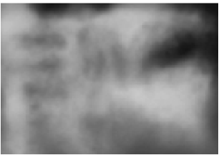
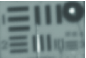
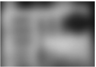
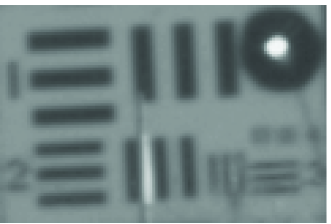
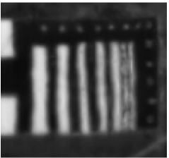
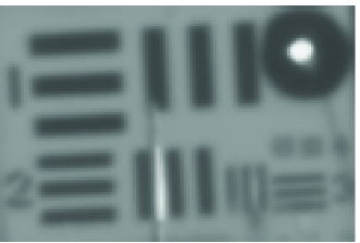
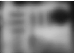
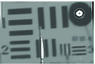
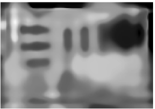
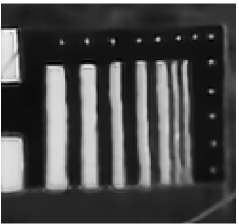
In Figure 2 we present the results for three data sets. For each one we show:

(A) a frame from the original data sequence;

(B) the temporal mean;

(C) the centroid $C$;

(D) the mean $C^{\mathrm{R}}$ of the images obtained by registering the data set onto the centroid;

(E) the image resulting from applying NL-TV to $C^{\mathrm{R}}$.

In fact we never use the temporal mean in our algorithm, but we show it here to emphasize how the centroid is generally much sharper and preserves more features than the temporal mean; this is especially true for data sets with intense turbulence, such as the one shown in the second column of Figure 2. We should note that while the centroid contains artifacts that are inherited by the particular image that is used to create it, this in not the case with the image $C^{\mathrm{R}}$ obtained by averaging the registered data. This is particularly apparent for the NATO sequence, shown in column (3) in Figure 2: note in particular how the second bar from the right has much more regular edges in image (D)-(3) than in image (C)-(3), and how some of the dots are better defined.

(1)                                                (2)                                        (3)

Figure 2: Results for three image sequences.

6 Current and future work

The geometric method that we have briefly described here proves quite effective for many data sets, such as the three that we have shown in this report. It is conceptually very simple and rather straightforward to implement. The results are comparable with the state of the art.

Perhaps the most fundamental issue that is currently being explored is the dependence of the centroid on the initial (reference) image, as we already discussed above; the procedure described at the end of section 3 (denoted with B) certainly alleviates the problem as it allows some of the possibly missing features to be recovered, but experimental results show that there is still a certain degree of dependence on the reference image. We are currently exploring algorithms to deal with this issue. Future work will also focus on speeding up the algorithm and selecting the parameters (e.g. in the computation of optical flow, or in the deconvolution step) in an automated manner.

7 Acknowledgements

The author’s research was partly supported by ONR grant N000140910256 and the KaraMetria program of the Agence Nationale de la Recherche (ANR) of France. I would like to thank Dr. Alan Van Nevel at the U.S. Naval Air Warfare Center, Weapons Division (China Lake, California) and the NATO SET156 (ex-SET072) Task Group for providing the image data. I am very grateful to Andrea Bertozzi, Jérôme Gilles, Yifei Lou, Stanley Osher, and Stefano Soatto of UCLA for introducing me to this research area in the first place and for the many lengthy discussions on the topic. I would also like to express my gratitude to Joan Alexis Glaunès of Université Paris Descartes for his advice and support during my stay at the MAP5 lab, and to Gabriel Peyré and François-Xavier Vialard of Université Paris Dauphine for their insightful suggestions. Last, but not least, the author is indebted to Xiaoqun Zhang, formerly at UCLA and now at Shanghai Jiaotong University, for providing very efficient nonlocal Total Variation (NL-TV) deconvolution code.

References

- [1] R. C. Aster, B. Borchers, and C. H. Thurber. Parameter Estimation and Inverse Problems. Academic Press, second edition, Feb. 2012.
- [2] J. L. Barron, D. J. Fleet, and S. S. Beauchemin. Performance of optical flow techniques. International Journal of Computer Vision, 12(1):43–77, Feb. 1994.
- [3] M. J. Black and P. Anandan. The robust estimation of multiple motions: Parametric and piecewise-smooth flow fields. Computer Vision and Image Understanding, 63(1):75–104, Jan. 1996.
- [4] L. C. Evans. Partial Differential Equations, volume 19 of Graduate Studies in Mathematics. American Mathematical Society, Providence, Rhode Island, 1998.
- [5] G. Gilboa and S. Osher. Nonlocal operators with applications to image processing. Multiscale Modeling and Simulation, 7(3):1005–1028, 2008.
- [6] J. Gilles, T. Dagobert, and C. De Franchis. Atmospheric turbulence restoration by diffeomorphic image registration and blind deconvolution. In Advanced Concepts for Intelligent Vision Systems, volume 5259 of Lecture Notes in Computer Science, pages 400–409. Springer-Verlag, 2008.
- [7] J. Gilles and Y. Mao. Non rigid geometric distortions correction – application to atmospheric turbulence stabilization. CAM Technical Report 10-86, UCLA Department of Mathematics, Dec. 2010.
- [8] J. Gilles and S. Osher. Fried deconvolution. CAM Technical Report 11-62, UCLA Department of Mathematics, Dec. 2011.
- [9] B. K. P. Horn and B. G. Schunck. Determining optical flow. Artificial Intelligence, 17(1–3):185–203, Aug. 1981.
- [10] B. K. P. Horn and B. G. Schunck. Determining optical flow: a retrospective. Artificial Intelligence, 59(1–2):81–87, Feb. 1993.
- [11] A. Kirsch. An Introduction to the Mathematical Theory of Inverse Problems, volume 120 of Applied Mathematical Sciences. Springer, Sept. 1996.
- [12] Y. Lou, X. Zhang, S. Osher, and A. Bertozzi. Image recovery via nonlocal operators. Journal of Scientific Computing, 2(42), Feb. 2010.
- [13] B. D. Lucas and T. Kanade. An iterative registration technique with an application to stereo vision. In Proceedings of the Seventh International Joint Conference on Artificial Intelligence (IJCAI), volume II, pages 674–679, Vancouver, B. C., Canada, Aug. 1981.
- [14] M. Shimizu, S. Yoshimura, M. Tanaka, and M. Okutomi. Super-resolution from image sequence under influence of hot-air optical turbulence. In Proceedings of the IEEE Conference on Computer Vision and Pattern Recognition (CVPR 2008), Anchorage, Alaska, June 2008.
- [15] A. Singh. Optic Flow Computation: A Unified Perspective. IEEE Computer Society Press, Los Alamitos, California, 1991.
- [16] D. Sun, S. Roth, and M. J. Black. Secrets of optical flow estimation and their principles. In Proceedings of the IEEE Conference on Computer Vision and Pattern Recognition (CVPR 2010), San Francisco, CA, June 2010.
- [17] C. Tomasi and T. Kanade. Detection and tracking of point features. Technical Report CMU-CS-91-132, Carnegie Mellon University, Apr. 1991.
- [18] X. Zhu and P. Milanfar. Image reconstruction from videos distorted by atmospheric turbulence. In SPIE Electronic Imaging, San Jose, CA, Jan. 2010.
- [19] X. Zhu and P. Milanfar. Stabilizing and deblurring atmospheric turbulence. In Proceedings of the of the IEEE International Conference on Computational Photography (ICCP 2011), Carnegie Mellon University, Pittsburgh, PA, Apr. 2011.