Dependence of the fragility of a glass former on the softness of interparticle interactions

Abstract

We study the influence of the softness of the interparticle interactions on the fragility of a glass former, by considering three model binary mixture glass formers. The interaction potential between particles is a modified Lennard-Jones type potential, with the repulsive part of the potential varying with an inverse power $q$ of the interparticle distance, and the attractive part varying with an inverse power $p$. We consider the combinations (12,11) (model I), (12,6) (model II) and (8,5) (model III) for (q,p) such that the interaction potential becomes softer from model I to III. We evaluate the kinetic fragilities from the temperature variation of diffusion coefficients and relaxation times, and a thermodynamic fragility from the temperature variation of the configuration entropy. We find that the kinetic fragility increases with increasing softness of the potential, consistent with previous results for these model systems, but at variance with the thermodynamic fragility, which decreases with increasing softness of the interactions, as well as expectations from earlier results. We rationalize our results by considering the full form of the Adam-Gibbs relation, which requires, in addition to the temperature dependence of the configuration entropy, knowledge of the high temperature activation energies ino rder to determine fragility. We show that consideration of the scaling of the high temperature activation energy with the liquid density, analyzed in recent studies, provides a partial rationalization of the observed behavior.

I Introduction

The temperature variation of relaxation times, viscosity and diffusion coefficient in glass forming liquids upon approaching the glass transition has been studied for a wide variety of substances. Near the glass transition, these quantities show a rapid increase, but with a rate of change that is different for different substances. The rapidity of rise of relaxation times near the glass transition has been quantified by “fragility”, introduced and analyzed extensively by Angell fragility_angell , which has proved to be useful in organizing and understanding the diversity of behavior seen in glass formers. Fragility has been defined in a variety of ways. Two of the popular definitions are in terms of the “steepness index” $m$, and the fragility defined using Vogel-Fulcher-Tammann (VFT) fits to viscosity and relaxation time data.

The steepness index of fragility is defined from the so-called Angell plot as the slope ($m$) of logarithm of the viscosity ($\eta$) or relaxation time ($\tau$) at $T=T_{g}$, with respect to the scaled inverse temperature $T_{g}/T$ where $T_{g}$ is the laboratory glass transition temperature:

$$m=\left(\frac{d\log\tau}{d(\frac{T_{g}}{T})}\right)_{T=T_{g}}$$ (1)

We refer to the fragilities defined from transport quantities and relaxation times as kinetic fragilities, to be distinguished from thermodynamic fragilities defined later. A kinetic fragility may also be defined from a VFT fit of the relaxation times,

$$\tau(T)=\tau_{0}\exp\left[\frac{1}{K_{VFT}(\frac{T}{T_{VFT}}-1)}\right]$$ (2)

which defines the kinetic fragility $K_{VFT}$ and the divergence temperature $T_{VFT}$.

Despite considerable research effort fragility_angell ; speedy ; pap:AG-Sastry ; wales ; tarjus ; ruocco ; sokolov ; pap:BordatPRL ; pap:BordatJNCS ; pap:Dudowicz-JPCB-2005 ; pap:Dudowicz-JCP-2005 ; douglas ; francis ; sneha ; tanaka ; pap:Mattsson-etal ; pap:Angell-news-views , and the observation of many empirical correlations between fragility and other material properties, a fully satisfactory understanding of fragility hasn’t yet been reached. Such understanding has been sought, broadly, along two lines. The first is a conceptual understanding of fundamental quantities that may govern fragility. An example of this kind is the use of the potential energy landscape approach in combination with Adam Gibbs (AG) relation AdamGibbs between relaxation time and configuration entropy [Eq. 3] to relate features of the energy landscape of a glass former to the fragility. The Adam-Gibbs relation

$$\tau(T)=\tau_{0}\exp(\frac{\delta\mu S^{*}k_{B}^{-1}}{TS_{c}})$$ (3)

relates the temperature dependence of the relaxation times to the temperature change in the configuration entropy $S_{c}$, where $\delta\mu$ is an activation free energy for particle rearrangements, and $S^{*}$ is the configurational entropy of cooperatively rearranging regions invoked in Adam-Gibbs theory. If $A\equiv\delta\mu S^{*}k_{B}^{-1}$ has no significant role to play in determining the fragility of a substance, it is the temperature variation of $TS_{c}$ that dictates the fragility. If the T-dependence of $S_{c}$ is given by

$$TS_{c}=K_{T}\left(\frac{T}{T_{K}}-1\right),$$ (4)

the Adam-Gibbs relation yields the VFT relation, with the identification $K_{VFT}=K_{T}/A$, $T_{VFT}=T_{K}$. Thus, $K_{T}$ is a thermodynamic index of fragility.

In what follows, we use Eq.s 2 and 3 which describe our simulation data well, as we demonstrate. However, our discussion does not depend crucially on the strict validity of the VFT temperature dependence near the glass transition, or the divergence of relaxation times at finite temperature; both these features have been questioned by various investigations and alternative forms to the VFT temperature dependence have been proposed Rossler ; Chandler ; Dyre .

In potential energy landscape approach pap:PEL-Sciortino ; pap:PEL-Heuer configuration entropy is associated with the number of local potential energy minima or inherent structures (IS) inh , and can be computed in terms of parameters describing the energy landscape pap:AG-Sastry . Hence thermodynamic fragility can be understood in terms of parameters of the potential energy landscape, namely the distribution of inherent structures and the dependence of the vibrational or basin entropy corresponding to inherent structures on theie energies. Although the exact temperature dependence of the configuration entropy depends on detailed properties of the distribution of inherent structures, and $K_{T}$ is not a constant even in the simplest case, such analysis does yield insight into the relationship between the energy landscape features and fragility. To a first approximation, the broader the distribution of energies of inherent structures, the larger the fragility of a glass former pap:AG-Sastry . Going beyond such analysis, one needs to also understand the behavior of the prefactor $A$, which is related to the high temperature activation energy tarjus ; schroder ; douglas ; ruocco . To the extent that the Adam-Gibbs relation quantitatively describes the temperature dependence of the relaxation times, such analysis provides a route to a fundamental understanding of fragility in terms of the phase space properties of a substance.

However, such a conceptual understanding does not directly address the dependence of fragility on specific, controllable material properties, an understanding that is desirable from the perspective, e. g., of materials design. The investigation of the dependence of fragility on the nature of molecular architecture and intermolecular interactions defines therefore a second distinct line of investigation, which has been pursued by various groups. For example, Dudowicz, Freed and Douglas pap:Dudowicz-JPCB-2005 ; pap:Dudowicz-JCP-2005 have investigated the role of backbone and side group stiffness in determining the fragility of polymer glass formers. In another recent example, from an experimental investigation on deformable colloidal suspensions, Mattsson et al pap:Mattsson-etal ; pap:Angell-news-views suggested that increasing the softness of the colloidal particles should decrease the fragility of the colloidal suspensions, and that such a principle should be more generally applicable. Indeed, this conclusion is consistent with that of Douglas and co-workers pap:Dudowicz-JPCB-2005 that the ability to better pack molecules leads to lower fragilities. In energy landscape terms, one may understand this conclusion as implying that molecules that pack well together will have narrower distributions of inherent structure energies.

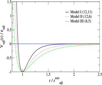
Figure 1: Comparison of interaction potential $V_{\alpha\beta}$ without truncation for the three different potentials used in the present study. $r^{min}_{\alpha\beta}$ are the positions of the minima of the interaction potentials.

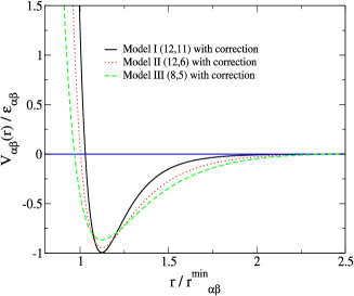
Figure 2: Comparison of the interaction potential $V_{\alpha\beta}$ with truncation for the three different potentials. $r^{min}_{\alpha\beta}$ are the positions of the minima of the interaction potentials.

The influence of the softness of interaction on the fragility was also investigated some time ago via computer simulations of model glass formers by Bordat et al  pap:BordatPRL ; pap:BordatJNCS . They considered a binary mixture of particles interacting via generalized Lennard Jones potentials, of the form

$$V(r)={\epsilon\over(q-p)}\left(p({\sigma\over r})^{q}-q({\sigma\over r})^{p}\right)$$ (5)

for combinations of the exponents $(q,p)$ of repulsive and attractive parts of the potential (12,11), (12,6) and (8,5). These combinations, corresponding to models labeled I, II and III, have decreasing curvatures at the minimum of the potential, and thus increasing softness. By evaluating the kinetic fragility of these models (the steepness index defined above), Bordat et al found that increasing softness of the interaction potential increases the kinetic fragility pap:BordatPRL ; pap:BordatJNCS .

The trend found by Bordat et al therefore is apparently not consistent with expectations arising from the other studies mentioned, although the nature of the changes in the interactions considered are not strictly the same. In order to understand better the relationship between the nature of the intermolecular interactions and fragility, in the present work we calculate the kinetic fragility $K_{VFT}$ using computer simulation data of the diffusion coefficient, and relaxation times obtained by a number of different means. We also calculate, using the procedure in pap:AG-Sastry ; pap:Sc-Sastry ; pap:Sc-Sastry-JPCM , the configuration entropy, from which we calculate a thermodynamic fragility ($K_{T}$). We find that these two fragilities show opposite trends, with the kinetic fragility increasing with softness, and the thermodynamic fragility decreasing with softness. In order to understand this apparent disagreement, we must consider the full form of the Adam-Gibbs relation, including terms that relate to the high temperature activation energy. We present our analysis along these lines below. We focus our analysis here on the role of a specific feature of the interaction potential, namely the softness, for reasons stated above. However, fragility in principle depends on a number of parameters that describe a glass former, which may include pressure, density etc.. While our study implicitly includes those factors that are affected by a change in the interaction potential (keeping other parameters fixed), we do not attempt here a comprehensive analysis of all factors that may influence the fragility of a glass former. Related questions concerning the change in structure, dynamics and thermodynamics in a glass forming liquid upon tuning the interaction potential have been addressed in pap:Shi-etal

The paper is organized as follows: In Section II we summarize the computer simulation details. In Section III we describe the methods used for evaluating the various quantities of interest. In Section IV we present our results and a discussion of the results, and Section V contains our conclusions.

II Simulation Details

We have studied a 80:20 binary mixture of modified Lennard Jones particles in three dimensions. The interaction potential is of the form given above in Eq. 5 with a truncation that makes both the potential and force go to zero smoothly at a cutoff distance $r_{c}$. The potential with the truncation is given by

$$V_{\alpha\beta}(r) = \frac{\epsilon_{\alpha\beta}}{q-p}\left[p(\frac{r_{\alpha\beta}^{min}}{r})^{q}-q(\frac{r_{\alpha\beta}^{min}}{r})^{p}\right]$$ (6)

$$+c_{1\alpha\beta}r^{2}+c_{2\alpha\beta},r<r_{c\alpha\beta}$$

$$= 0,\hskip 14.22636pt\mbox{otherwise}$$

where $\alpha,\beta\in\{A,B\}$. $r_{\alpha\beta}^{min}=2^{\frac{1}{6}}\sigma_{\alpha\beta}$ and $\epsilon_{\alpha\beta}$ are respectively the position and the value of the minimum of the pair potential. The correction terms $c_{1\alpha\beta},c_{2\alpha\beta}$ are determined from the conditions :

$$V_{\alpha\beta}(r_{c\alpha\beta}) = 0$$

$$\left(\frac{dV_{\alpha\beta}}{dr}\right)_{r_{c\alpha\beta}} = 0$$ (7)

The energy and size parameters $\epsilon_{\alpha\beta}$ and $\sigma_{\alpha\beta}$ correspond to those of the Kob-Andersen binary Lennard-Jones model kob . Units of length, energy and time scales are $\sigma_{AA},\epsilon_{AA}$ and $\sqrt{\frac{\sigma_{AA}^{2}m_{AA}}{\epsilon_{AA}}}$ respectively. In this unit, $\epsilon_{AB}=1.5$, $\epsilon_{BB}=0.5$, $\sigma_{AB}=0.80$, $\sigma_{BB}=0.88$. The interaction potential was cutoff at $2.5\sigma_{\alpha\beta}$, The three different models $(12,11)$, $(12,6)$ and $(8,5)$ are shown without and with cutoff in Fig.s 1 and 2. Molecular dynamics (MD) simulations were done in a cubic box with periodic boundary conditions in the constant nummber, volume and temperature (NVT) ensemble. The integration time step was in the range $dt=0.001-0.005$. Temperatures were kept constant using an algorithm due to Brown and Clarke pap:BC . Simulations were done in the temperature range $T\in\left[0.85,5\right]$ for $(12,11)$; $T\in\left[0.45,5\right]$ for $(12,6)$ and $T\in\left[0.23,5\right]$ for $(8,5)$ model respectively. System size were $N=1500,N_{A}=1200$ ($N=$ total number of particles, $N_{A}=$ number of particles of species $A$) and the number density was $\rho=1.2$ (pap:BordatPRL , see also Fig. 3). For all models, one sample per state point above the onset temperature (described below) and three to five samples per state points below the onset temperature were used with runlengths $>100\tau_{\alpha}$ ($\tau_{\alpha}$ is the relaxation time, described below).

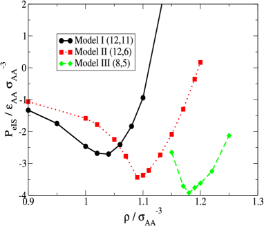
Figure 3: Pressure vs. density for inherent structures (IS). The density minimum for IS pressure occurs at $\rho=1.04,1.09,1.18$ respectively for models I $(12,11)$, II $(12,6)$, and III $(8,5)$. This density defines the lower bound for simulations of the system in the homogeneous liquid state.

III Methods

In this section, we describe the various quantities that have been calculated and the methods employed for such calculations.

III.1 The $\alpha$ relaxation time

The following measures have been used to extract $\alpha$ relaxation times:

1. Diffusion coefficient ($D_{A}$) from the mean squared displacement (MSD) of the $A$ type particles.

2. Relaxation times obtained from the decay of overlap function $q(t)$ using the definition $q(t=\tau_{\alpha},T)/N=1/e$. The overlap function is a two-point time correlation function of local density pap:4pt-CD ; pap:Ovlap-Glotzer-etal ; pap:Ovlap-Donati-etal ; pap:Lacevic ; pap:Karmakar-PNAS which has been used in many recent studies of slow relaxation, and is defined as:

   $$<q(t)> \equiv <\int d\vec{r}\rho(\vec{r},t_{0})\rho(\vec{r},t+t_{0})>$$ (8)

   $$= <\sum_{i=1}^{N}\sum_{j=1}^{N}\delta(\vec{r}_{j}(t_{0})-\vec{r}_{i}(t+t_{0}))>$$

   Here the averaging over time origins $t_{0}$ is implied. The overlap function naturally separates into “self” and “distinct” terms:

   $$<q(t)> = <\sum_{i=1}^{N}\delta(\vec{r}_{i}(t_{0})-\vec{r}_{i}(t+t_{0}))>$$

   $$+<\sum_{i}\sum_{j\neq i}\delta(\vec{r}_{i}(t_{0})-\vec{r}_{j}(t+t_{0}))>$$

   In our work, we consider only the self part of the total overlap function (i.e. neglect the $i\neq j$ terms in the double summation), based on the observation pap:Lacevic that the results obtained from the self part are not significantly different from those obtained by considering the collective overlap function. Thus we use

   $$<q(t)> \approx <\sum_{i=1}^{N}\delta(\vec{r}_{i}(t_{0})-\vec{r}_{i}(t+t_{0}))>$$

   Further, for numerical computation, the $\delta$ function is approximated by a window function $w(x)$ which defines the condition of “overlap” between two particle positions separated by a time interval $t$:

   $$<q(t)> \approx <\sum_{i=1}^{N}w(|\vec{r}_{i}(t_{0})-\vec{r}_{i}(t_{0}+t)|)>$$

   $$w(x) = 1,x\leq a\textnormal{ implying ``overlap''}$$

   $$= 0\mbox{ otherwise }$$

   The time dependent overlap function thus depends on the choice of the cutoff parameter $a$, which we choose to be $0.3$. This parameter is chosen such that particle positions separated due to small amplitude vibrational motion are treated as the same, or that $a^{2}$ is comparable to the value of the MSD in the plateau between the ballistic and diffusive regimes.

3. We have also studied the “susceptibility” $\chi_{4}(t)$, defined in terms of the fluctuations in the overlap function as

   $$\chi_{4}(t)={1\over N}\left(\langle q(t)^{2}\rangle-\langle q(t)\rangle^{2}\right)$$ (9)

   This quantity can be written as an integral of a higher order, four point correlation function $g_{4}(\vec{r},t)$ pap:4pt-CD ; pap:Ovlap-Glotzer-etal ; pap:Ovlap-Donati-etal widely studied in the context of dynamical heterogeneity:

   $$g_{4}(\vec{r},t) = \langle\rho(0,0)\rho(\vec{r},0)\rho(0,t)\rho(\vec{r},t)\rangle-$$

   $$\langle\rho(0,0)\rho(\vec{r},0)\rangle\langle\rho(0,t)\rho(\vec{r},t)\rangle$$

   $$\chi_{4}(t) = \int d\vec{r}g_{4}(\vec{r},t)$$ (10)

   The characteristic time $\tau_{4}(T)$ at which the fluctuation ($\chi_{4}(t)$) is maximum is taken as a measure of relaxation time.

4. Relaxation times obtained from the decay of the self intermediate scattering function $F_{s}(k,t)$ using the definition $F_{s}(k,t=\tau_{\alpha},T)=1/e$ at $k\simeq\frac{2\pi}{r_{min}}$. The self intermediate scattering function is calculated from the simulated trajectory as:

   $$F_{s}(k,t)=\frac{1}{N}\langle\sum_{i=1}^{N}\exp\left(-\imath\vec{k}\cdot(\vec{r}_{i}(t)-\vec{r}_{i}(0))\right)\rangle$$ (11)

Since the relaxation times from $q(t)$, $\chi_{4}(t)$ and $F_{s}(k,t)$ behave very similarly, we discuss further only the time scale obatined from $q(t)$.

III.2 Characteristic temperature scales

Dynamics of fragile glass forming liquids show characteristic cross-over from high temperature Arrhenius behaviour to low temperature super Arrhenius behaviour at some characteristic temperature. At this temperature, systems also show cross-over from a “landscape independent” high temperature regime to a “landscape influenced” low temperature regime pap:sastry-deb-stil ; pap:Sastry-pcc . We denote this temperature as onset temperature $T_{onset}$. We report the estimates from inherent structure energies in Table 1. As the temperature is further lowered, mode coupling theory predicts divergence of relaxation time $\tau$ as $\tau(T)\sim(T-T_{c})^{-\gamma}$ which defines the mode coupling divergence temperature $T_{c}$ which we estimate from both relaxation time and diffusion coefficient (in the form $(D_{A}/T)^{-1}$) kob . Similarly relaxation times apparently diverge at a second characteristic temperature which we estimate from VFT fits and denote as $T_{VFT}$. Further, configuration entropy becomes zero on extrapolation at a characteristic temperature (Eq. 4) known as Kauzmann temperature ($T_{K}$). The AG relation (Eq. 3) predicts that these two temperatures ($T_{VFT}$ and $T_{K}$) to be same. Although we use functional forms that have a temperature of vanishing $S_{c}$ and diverging relaxation times, these are employed as useful descriptions of the data, without any implied assertion of the expected behavior at temperatures lower than the ones we study. The The values of different characteristic temperatures for different potentials are tabulated in Table 1.

Table 1: Characteristic Temperatures

Quantity	(12,11)	(12,6)	(8,5)
$T_{onset}$	1.27	0.9	0.42
$T_{c}$ from $(\frac{D_{A}}{T})^{-1}$	0.77	0.42	0.22
$T_{c}$ from $q(t)$	0.77	0.42	0.23
$T_{VFT}$ from $(\frac{D_{A}}{T})^{-1}$	0.59	0.32	0.17
$T_{VFT}$ from $q(t)$	0.55	0.29	0.16
$T_{K}$	0.54	0.28	0.16

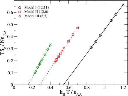
Figure 4: Temperature dependence of $TS_{c}$ for the studied models to determine the Kauzmann temperature. $T_{K}=0.54,0.28,0.16$ respectively for models I $(12,11)$, II $(12,6)$, and III $(8,5)$. The value of $T_{K}$ from the extrapolated crossing of bulk and basin entropies vs. temperature reported in  pap:Sc-Sastry-JPCM is $T_{K}=0.2976$ and in  thesis:Karmakar is $T_{K}\sim 0.29$. The $T_{K}$ values obtained from this plot is used to determine the thermodynamic fragility in Fig. 5.

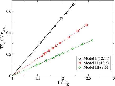
Figure 5: Determination of the thermodynamic fragility from the relation $TS_{c}=K_{T}(\frac{T}{T_{K}}-1)$ for the studied models. $K_{T}$ is the slope of the linear fit shown. $T_{K}$ is the temperature at which $S_{c}=0$, obtained from the linear fit shown in Fig. 4. Thermodynamic fragility ($K_{T}$) values are $0.551,0.323,0.211$ for models I $(12,11)$, II $(12,6)$, and III $(8,5)$ respectively

III.3 Configuration entropy

Configuration entropy ($S_{c}$) per particle, the measure of the number of distinct local energy minima, is calculated pap:Sc-Sastry by subtracting from the total entropy of the system the “vibrational” component:

$$S_{c͑}(T)=S_{total}(T)-S_{vib}(T)$$ (12)

The total entropy of the liquid is obtained via thermodynamic integration from the ideal gas limit. Vibrational entropy is calculated by making a harmonic approximation to the potential energy about a given local minimum pap:Sc-Sastry ; pap:Sc-Sastry-JPCM ; pap:PEL-Sciortino ; pap:PEL-Heuer . The procedure used for generating local energy minima, and calculating the vibrational entropy is as outlined in pap:Sc-Sastry ; pap:Sc-Sastry-JPCM .

We have also computed the configuration entropy density $S_{c}(e_{IS})=k_{B}\ln\Omega(e_{IS})$ where $\Omega(e_{IS})$ is the number density of inherent structures with energy $e_{IS}$ and to a good approximation may be described by a Gaussian. Equivalently, $S_{c}(e_{IS})$ can be described by a parabola

$$S_{c}(e_{IS})=\alpha-\frac{(e_{IS}-e_{IS}^{0})^{2}}{\sigma^{2}}$$ (13)

The parameter $\alpha$ denotes the peak value of $S_{c}(e_{IS})$ which occurs at energy $e_{IS}^{0}$. $S_{c}(e_{IS})$ is zero at $e_{IS}=e_{IS}^{0}\pm\sigma\sqrt{\alpha}$. Thus $\sigma\sqrt{\alpha}$ is a measure of the spread of $S_{c}(e_{IS})$. We denote the lower root $e_{IS}^{0}-\sigma\sqrt{\alpha}$ by $e_{IS}^{min}$.

In the harmonic approximation to vibrational entropy, the average value of IS energy sampled by a system at a given temperature $<e_{IS}>(T)$ is predicted to be linear in inverse temperature $\beta=1/T$:

$$\langle e_{IS}\rangle(T)=\langle e_{IS}\rangle(\infty)-\frac{\sigma^{2}}{2T}$$ (14)

where $\langle e_{IS}\rangle(\infty)$ is the extrapolated limiting value of $\langle e_{IS}\rangle$ at high temperatures. These parameters which characterizes the potential energy landscape are tabulated in Table 2 for different potentials.

IV Results and Discussion

The results from the simulations concerning the thermodynamic and kinetic fragility estimates are presented below.

IV.1 Thermodynamic fragility

As described in the Introduction, we may define a thermodynamic fragility $K_{T}$ as the slope of $TS_{c}(T)$ vs. $T/T_{K}$. Fig. 4 shows that indeed, $TS_{c}(T)$ varies linearly with temperature, which allows us to define $T_{K}$. The $T_{K}$ values for the different potentials are listed in Table 1. Various quantities related to the distribution of inherent structure energies are listed in Table II for later use. Thermodynamic fragility $K_{T}$ as defined in Eq.  4 is computed from the slope of $TS_{c}$ vs. $T/T_{K}$ is found to decrease as the softness of the interaction potential increases, as shown in Fig. 5. Such behavior is in line with expectations, e. g. from pap:Mattsson-etal ; pap:Dudowicz-JPCB-2005 .

IV.2 Kinetic fragility

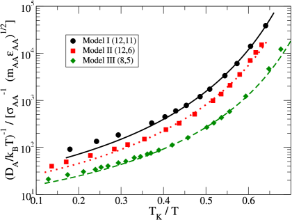
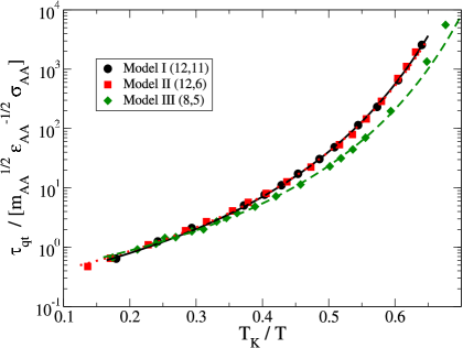
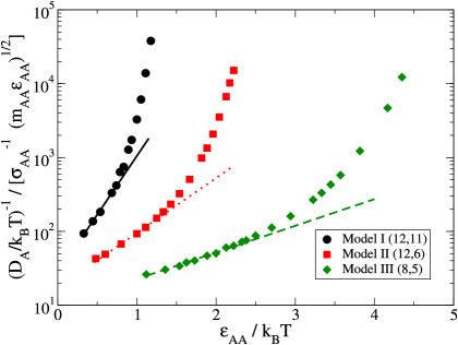
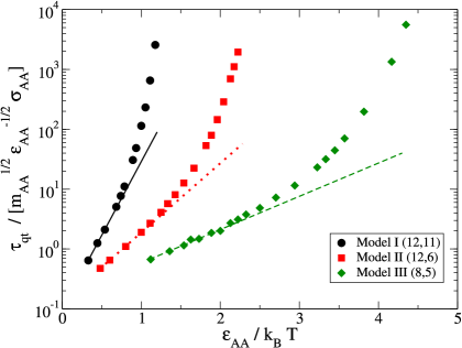
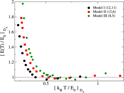
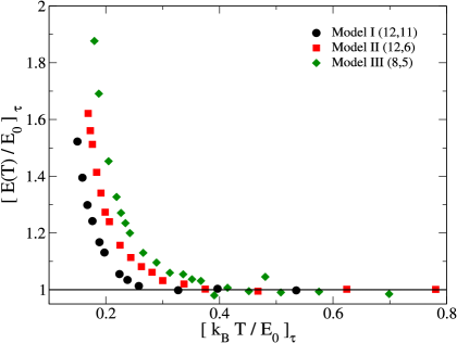
Figure 6: Top row: Inverse diffusion coefficient and relaxation time from overlap function vs. scaled inverse temperature $\frac{T_{K}}{T}$. Lines through the data show VFT fits to the data below the onset temperature. $T_{K}$ estimated from fig. 4 are used as the divergence temperatures in the VFT fits. Middle row: Arrhenius fits to high temperature data of inverse diffusion coefficient and relaxation time from overlap function to determine high temperature activation energies $E_{0}$. Bottom row: effective activation energy $E(T)$ (see text) scaled by $E_{0}$, plotted against $k_{B}T/E_{0}$.

Kinetic fragility ($K_{VFT}$) is estimated by fitting to the VFT form Eq.  2 the diffusion coefficients and relaxation times.

In Fig  6 (top panels), we show the Arrhenius plot of the diffusion coefficients and relaxation times from $q(t)$, plotted against $T_{K}/T$. The VFT divergence temperatures $T_{VFT}$, obtained from VFT fits to the data for temperatures below the onset temperature, are found to be close to $T_{K}$ and are listed in Table I. The middle panels of Fig  6 show Arrhenius fits to high temperature data (above the onset temperature), from which activation energies $E_{0}$ (such that $\tau(T)=\tau_{0}\exp(E_{0}/k_{B}T)$ are obtained. These are listed in Table III, and will be discussed later. In the bottom panels of Fig  6, we show the effective activation energy defined as $E(T)\equiv k_{B}T\ln(\tau(T)/\tau_{0})$ scaled by $E_{0}$ (similarly for $D_{A}/T$), plotted against $k_{B}T/E_{0}$.

We note in the passing that for model $(12,6)$ the proportionality $E_{0}\sim 6T_{c}$ pap:Dudowicz-JPCB-2005 is reasonably well satisfied. However, the ratio $E_{0}/T_{c}$ decreases from $\sim 7$ to $\sim 5$ as softness increases.

Next, we calculate the kinetic fragilities $K_{VFT}$, from diffusion coefficients and relaxation times, using the divergence temperature $T_{VFT}$ obtained with $T_{VFT}$ as a fit parameter, as well as using $T_{K}$ estimates from the configuration entropy as the divergence temperatures. The corresponding kinetic fragilities, labeled $K_{VFT}^{I}$ and $K_{VFT}^{II}$, are listed in Table IV, along with the thermodynamic fragilities $K_{T}$. We find that the kinetic fragilities increase as the softness of the interaction potential increases, thus showing a trend that is opposite to that of the thermodynamic fragility.

IV.3 Adam Gibbs relation and fragility

In order to understand this discrepancy, we consider again the Adam-Gibbs relation, which relates the kinetic and thermodynamic fragilities. Comparing Eq. 2, Eq. 3 and Eq. 4, we note that the relationship between the kinetic and thermodynamic fragilities that we may deduce assuming the validity of the VFT and the AG relations is

$$K_{VFT}=K_{T}/A$$ (15)

and we expect at least the same trend in the two fragilities under the assumption that the term $A$ does not substantially alter the proportionality between kinetic and thermodynamic fragilities. To assess the degree to which this is true in our models, we show in Fig. 7 the Adam-Gibbs plots of the diffusion coefficient and relaxation times. These plots show that the coefficient $A$, obtained from the slopes (and listed in Table III), indeed varies from one model to the other, decreasing as the softness increases. Thus, the ratio $K_{T}/A$ shows the opposite trend, increasing as the softness increases.

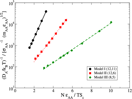
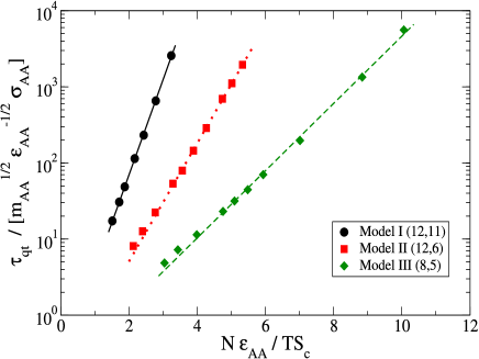
Figure 7: Adam Gibbs plots for the inverse diffusion coefficient of $A$ particles and relaxation time from overlap function, for the three models studied. The activation energy parameter $A$ in Eq. 3, obtained from the slopes of the data shown, is tabulated in table 3.

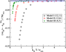
Figure 8: Temperature dependence of the inherent structure energy $e_{IS}$ for the studied models shifted by the corresponding high temperature limiting values $e_{IS}^{lim}$ for clarity. The values of $e_{IS}^{lim}$ are $-6.003,-6.886,-7.191$ for models I $(12,11)$, II $(12,6)$ and III $(8,5)$ respectively.

We next attempt to understand the dependence of the Adam-Gibbs coefficient $A$ on the softness of the interaction. First we consider the high temperature Arrhenius behavior of relaxation times, in terms of the Adam-Gibbs relation. Such Arrhenius behavior can be expected if the configuration entropy effectively becomes a constant, in which case, the high temperature activation energy will be given by

$$E_{0}=Ak_{B}/Sc_{\infty}$$ (16)

However, the asymptotic high temperature configuration entropy is difficult to assess directly, as the various available approaches to computing the basin entropy do not work well in this regime(see e. g. pap:Sastry-pcc ). We thus use the following procedure: First, we determine directly from simulations the high temperature limit of the inherent structure energies, $e_{IS}^{lim}$ (see Fig. 8). Then, we use the extrapolation of the dependence of the configuration entropy $S_{c}$ on the inherent structure energy $e_{IS}$ obtained below the onset temperature to obtain the high temperature limit of the configuration entropy, $S_{c}(e_{IS}^{lim})$, which do not vary appreciably with softness of interaction, and are listed in Table II. Table II also lists $S_{c}(\infty)$, the infinite temperature value of $S_{c}$ obtained by extrapolating Eq. 4 to infinite temperature, a procedure that is not justified at temperatures above the onset temperature. Using these $S_{c}(e_{IS}^{lim})$ values, and the activation energies $E_{0}$ shown in Table III, we obtain estimates for the AG coefficient

$$A_{est}=E_{0}S_{c}(e_{IS}^{lim})/k_{B}$$ (17)

which are shown in Table III. We note in Table III that $E_{0}$ values decrease strongly as the softness of the interactions increases, and with a corresponding moderate increase of $S_{c}(e_{IS}^{lim})$, our estimates of $A_{est}$ agree rather well with the values obtained directly from the Adam-Gibbs plots. We now designate the thermodynamic fragility estimates obtained by considering the full form of the Adam-Gibbs relation as $K_{AG}=K_{T}/A$, and list them along side the thermodynamic and kinetic fragility estimates in Table IV. As expected from the above discussion, the “Adam-Gibbs” fragility estimates ($K_{AG}^{I}$ in Table IV) agree rather well with the kinetic fragilities.

Although the above picture provides a consistent description of the fragilities from kinetic and thermodynamic data, a question remains regarding the variation of the high temperature activation energy $E_{0}$ with the softness of the interaction potential. To seek some insight into this question, we consider work in recent years concerning the scaling of the temperature dependence of dynamic and thermodynamic quantities at different densities schroder ; tarjus ; roland . It has been shown by many groups that a scaled variable $\rho^{\gamma}/T$, where $\rho$ is the density, captures the density variation of properties in many liquids. The exponent $\gamma$ can easily be shown to be $n/3$ for inverse power law potentials, where $n$ is the power of the inverse power law, but even for other liquids, an effective $\gamma$ has been shown to be derivable by considering the correlated fluctuations of potential energy and the virial schroder . The exponent $\gamma$ is obtainable as the ratio of fluctuations. Although such a ratio is state point dependent, a “best fit” value, typically obtained from high temperature state points, has been shown to effectively describe the scaling of properties at different densities. Since we do not perform a full analysis of the density dependence here, we do not estimate the best value of $\gamma$ but instead use the value at twice the onset temperature as an indicative value. Fig. 9 shows the fluctuation data from which the $\gamma$ value is obtained, and the temperature variation of the exponents. The values of $\gamma$ we use are shown in Table II.

Based on the above considerations, we should expect the high temperature activation energies to be proportional to $\rho^{\gamma}$. Accordingly, we obtain estimates of the activation energy in the form $E_{0}=E_{00}\rho^{\gamma}$. These values, shown in Table III, have a weaker temperature dependence than the directly evaluated $E_{0}$, and correspondingly, the fragility estimates obtained (shown in Table IV), while showing a smaller decrease with softness, nevertheless decrease with increasing softness of interaction. A further analysis is needed, therefore, to elucidate the relevance of these considerations to evaluating the variation of the high temperature activation energy.

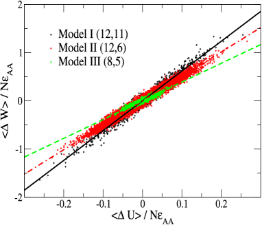
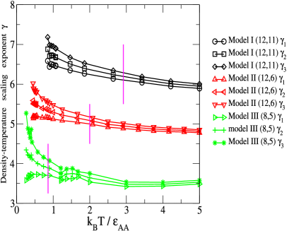
Figure 9: Determination of the density-temperature scaling exponent $\gamma$ from the correlation between instantaneous potential energy ($U$) and virial ($W$). $\gamma_{1}=\frac{\langle\Delta W\Delta U\rangle}{\langle(\Delta U)^{2}\rangle}$, $\gamma_{2}=\frac{\sqrt{\langle(\Delta W)^{2}}}{\sqrt{\langle(\Delta U)^{2}\rangle}}$, $\gamma_{3}=\frac{\langle(\Delta W)^{2}\rangle}{\langle\Delta W\Delta U\rangle}$ where $\Delta U=U-\langle U\rangle$ and $\Delta W=W-\langle W\rangle$ represent fluctuations about mean of potential energy and virial respectively. The left panel shows the correlation between energy and virial at temperatures $\approx 2T_{onset}$, with straight line fits $\langle\Delta W\rangle=\gamma_{2}(2T_{onset})\langle\Delta U\rangle$. The right panel shows the temperature dependent values of $\gamma$ for the studied models.

V Conclusions

We have studied the effect of the softness of the interaction potential on fragility in three model glass formers. We find that the kinetic fragility obtained from diffusion coefficients and relaxation times increases with increasing softness of the interaction potential, contrary to expectations based on earlier studies pap:Mattsson-etal ; pap:Dudowicz-JPCB-2005 . On the other hand, a thermodynamic fragility obtained from the temperature variation of the configuration entropy decreases with increasing softness of the interaction potential. By taking into consideration the model dependence of the high temperature activation energy, in addition to the temperature dependence of the configuration entropy, we define an “Adam-Gibbs” fragility whose model dependence accurately captures the variation of the kinetic fragilities that we find. An attempt to rationalize the model dependence of the high temperature in terms of the scaling of properties with respect to density is encouraging but fails to fully explain the observed decrease of the fragility with increasing softness of the interaction potential.

Table 2: Potential energy landscape parameters and density temperature scaling exponents for the studied models. Fit forms used: $\langle e_{IS}\rangle(T)=\langle e_{IS}\rangle(\infty)-\frac{\sigma^{2}}{2T}$; $S_{C}(e_{IS})=\alpha-\frac{(e_{IS}-e_{IS}^{0})^{2}}{\sigma^{2}}$.

Quantity	(12,11)	(12,6)	(8,5)
Density minimum for IS pressure	1.04	1.09	1.18
Height of $S_{C}(e_{IS})$ distribution $\alpha$	0.863	0.886	0.905
Spread of $S_{C}(e_{IS})$ distribution $\alpha^{1/2}\sigma$	0.816	0.455	0.255
IS Energy where $S_{C}(e_{IS})=0$, $e_{IS}^{min}=e_{IS}^{0}-\sigma\sqrt{\alpha}$	-6.457	-7.132	-7.346
$\langle e_{IS}\rangle(\infty)$	-5.761	-6.734	-7.098
Limiting value of IS energy $e_{IS}^{lim}$	-6.003	-6.886	-7.191
$S_{c}(e_{IS}^{lim})$	0.69	0.7	0.78
$S_{c}(\infty)=\frac{K_{T}}{T_{K}}$	1.01	1.14	1.35
Density temperature scaling exponent at $2\times T_{onset}$
$\gamma_{1}$	6.09	4.99	3.71
$\gamma_{2}$	6.18	5.07	3.89
$\gamma_{3}$	6.27	5.15	4.09
$\rho^{\gamma_{1}}=1.2^{\gamma_{1}}$	3.04	2.48	1.97
$\rho^{\gamma_{2}}=1.2^{\gamma_{2}}$	3.09	2.52	2.03
$\rho^{\gamma_{3}}=1.2^{\gamma_{3}}$	3.14	2.56	2.11

Table 3: Comparison of activation energy parameters. $A$ is the activation parameter in the Adam Gibbs (AG) relation. $E_{0}$ is the high temperature activation energy in Arrhenius fit. $S_{c}(e_{IS}^{lim})$ is the values of configuration entropy density at the limiting value of inherent structure energies at high temperatures. $A_{est}^{I}=E_{0}S_{c}(e_{IS}^{lim})/k_{B}$ is the expected value of parameter $A$ obtained from $E_{0}$. $E_{0}^{est}=E_{00}\rho^{\gamma}$ is the estimate of $E_{0}$ from density - temperature scaling of relaxation time where $\gamma_{2}$ are the values of the scaling exponent at twice the onset temperature. $A_{est}^{II}=E_{0}^{est}S_{c}(e_{IS}^{lim})$ is the expected value of energy barrier $A$ obtained from $E_{0}^{est}$.

	From $q(t)$						From $(\frac{D_{A}}{T})^{-1}$
Model
	$A$	$E_{0}$	$A_{est}^{I}$	$E_{00}$	$E_{0}^{est}$	$A_{est}^{II}$	$A$	$E_{0}$	$A_{est}^{I}$	$E_{00}$	$E_{0}^{est}$	$A_{est}^{II}$
(12,11)	2.88	5.67	3.91		4.13	2.85	2.27	3.65	2.52		2.63	1.81
(12,6)	1.79	2.67	1.87	1.34	3.38	2.40	1.35	1.71	1.20	0.85	2.14	1.52
(8,5)	1.02	1.28	1.00		2.72	2.12	0.71	0.83	0.65		1.73	1.35

Table 4: Comparison of fragility parameters. $K_{T}$ is thermodynamic fragility obtained from temperature dependence of $TS_{c}(T)$. $K_{VFT}^{I}$ is kinetic fragility from VFT fit and $K_{VFT}^{II}$ is kinetic fragility obtained from VFT fit assuming $T_{VFT}=T_{K}$. $K_{AG}^{I}=\frac{K_{T}}{A_{est}^{I}}$ is the fragility expected from high temperature activation energy $E_{0}$ obtained from an Arrhenius fit. $K_{AG}^{II}=\frac{K_{T}}{A_{est}^{II}}$ where the high temperature activation energy is estimated from density-temperature scaling.

		From $q(t)$				From $(\frac{D_{A}}{T})^{-1}$
Model
	$K_{T}$	$K_{VFT}^{I}$	$K_{VFT}^{II}$	$K_{AG}^{I}$	$K_{AG}^{II}$	$K_{VFT}^{I}$	$K_{VFT}^{II}$	$K_{AG}^{I}$	$K_{AG}^{II}$
(12,11)	0.551	0.20	0.19	0.14	0.19	0.34	0.24	0.22	0.30
(12,6)	0.323	0.21	0.20	0.17	0.13	0.38	0.26	0.27	0.21
(8,5)	0.211	0.26	0.23	0.21	0.10	0.40	0.32	0.32	0.16

References

- (1) C. A. Angell, J. Non-Cryst. Solids 131-133, 13 (1991); R. Böhmer, K. L. Ngai, C. A. Angell and D. J. Plazek, J. Chem. Phys. 99, 4201 (1993); C. A. Angell, Science, 267, 1924 (1995);
- (2) R. J. Speedy, J. Phys. Chem. B 103, 4060 (1999).
- (3) S. Sastry, Nature 409, 164 (2001).
- (4) D. J. Wales and J. P. K. Doye Phys. Rev. B 63, 214204 (2001); vol. 64, 024205 (2001).
- (5) C. Alba-Simionesco, D. Kivelson, and G. Tarjus, J. Chem. Phys. 116, 5033 (2002); G. Tarjus, D. Kivelson, S. Mossa and C. Alba-Simionesco, J. Chem. Phys. 120, 6135 (2004); C. Alba-Simionesco, A. Cailliaux, A. Alegría and G. Tarjus, Europhys. Lett., 68, 58, (2004).
- (6) G. Ruocco, F. Sciortino, F. Zamponi, C. De Michele and T. Scopigno, J. Chem. Phys., 120, 10666 (2004).
- (7) V. N. Novikov and A. P. Sokolov, Nature 431, 961 (2004).
- (8) P. Bordat, F. Affouard, M. Descamps, Phys. Rev. Lett. 93, 105502 (2004).
- (9) P. Bordat, F. Affouard, M. Descamps, J. Non Cryst. Solids 353, 3924 (2007).
- (10) J. Dudowicz, K. F. Freed and J. F. Douglas, J. Phys. Chem. B 109, 21350 (2005).
- (11) J. Dudowicz, K. F. Freed and J. F. Douglas, J. Chem. Phys. 123, 111102 (2005).
- (12) J. F. Douglas, J. Dudowicz and K. F. Freed, J. Chem. Phys. 125, 144907 (2006); R. A. Riggleman, J. F. Douglas and J. J. de Pablo, J. Chem. Phys. 126, 234903 (2007).
- (13) F. W. Starr and J. F. Douglas, Phys. Rev. Lett. 106 115702 (2011).
- (14) S. E. Abraham, S. M. Bhattacharrya, and B. Bagchi, Phys. Rev. Lett. 100, 167801 (2008).
- (15) H. Shintani and H. Tanaka, Nat. Mater. 7, 870 (2008).
- (16) Johan Mattsson, Hans M. Wyss, Alberto Fernandez-Nieves, Kunimasa Miyazaki, Zhibing Hu, David R. Reichman and David A. Weitz, Nature (London), 462, 83 (2009).
- (17) C. A. Angell and K. Ueno, Nature 462, 45, (2009).
- (18) G. Adam and J. H. Gibbs, J. Chem. Phys. 43, 139 (1965).
- (19) E. Rossler, K.-U. Hess, V. N. Novikov, J. Non-Cryst. Solids 223, 207 (1998).
- (20) Y. S. Elmatad, D. Chandler, and J. P. Garrahan, J Phys Chem B 114, 17113 (2010); and J. Phys. Chem. B. 113, 5563 (2009).
- (21) T. Hecksher, A. I. Nielsen, N. B. Olsen And J. C. Dyre, Nature Physics 4 737 (2008).
- (22) F. Sciortino, J. Stat. Mech. P05015 (2005).
- (23) A. Heuer, J. Phys.: Condens. Matter 20, 373101 (2008).
- (24) F. H. Stillinger and T. A. Weber, Science 225,983 (1984); F. H. Stillinger, Science 267, 1935 (1995).
- (25) Nicoletta Gnan, Thomas B. Schrøder, Ulf R. Pedersen, Nicholas P. Bailey, and Jeppe C. Dyre, J. Chem. Phys. 131, 234504 (2009); Thomas B. Schrøder, Nicoletta Gnan, Ulf R. Pedersen, Nicholas P. Bailey, and Jeppe C. Dyre, J. Chem. Phys. 134, 164505 (2011) and other papers in the series.
- (26) S. Sastry, Phys. Rev. Lett. 85, 590 (2000).
- (27) S. Sastry, J. Phys.: Condens. Matter 12, 6515 (2000).
- (28) W. Kob and H. C. Andersen, Phys. Rev. E 51, 4626 (1995).
- (29) D. Brown and J. H. R. Clarke, Mol. Phys. 51, 1243 (1984).
- (30) C. Dasgupta, A. V. Indrani, S. Ramaswamy and M. K. Phani, Europhys. Lett. 15, 307 (1991).
- (31) S. C. Glotzer, V. N. Novikov and T. B. Schrøder, J. Chem. Phys. 112, 509 (2000).
- (32) N. Lac̆ević, F. W. Starr, T. B. Schrøder, and S. C. Glotzer, J. Chem. Phys. 119, 7372 (2003).
- (33) C. Donati, S. Franz, S. C. Glotzer and G. Parisi, J. Non-Cryst Solids 307, 215–224 (2002).
- (34) S. Karmakar, C. Dasgupta, S. Sastry, Proc. Natl. Acad. Sci. (US) 106, 3675, (2009).
- (35) S. Sastry, P. G. Debenedetti and F. H. Stillinger, Nature 393, 554 (1998).
- (36) S. Sastry, PhysChemComm, 3, 79, (2000).
- (37) S. Karmakar, Ph. D. Thesis (2008).
- (38) C. M. Roland, S. Hensel-Bielowka, M. Paluch and R. Casalini, Rep. Prog. Phys. 68, 1405 (2005); C. M. Roland, Macromolecules 43, 7875 (2010).
- (39) Z. Shi, P. G. Debenedetti, F. H. Stillinger and P. Ginart, J. Chem. Phys. 135, 084513 (2011).