Reexamination of the Infrared Excess–Ultraviolet Slope Relation of
Local Galaxies

Abstract

The relation between the ratio of infrared (IR) and ultraviolet (UV) flux densities (the infrared excess: IRX) and the slope of the UV spectrum ($\beta$) of galaxies plays a fundamental role in the evaluation of the dust attenuation of star forming galaxies especially at high redshifts. Many authors, however, pointed out that there is a significant dispersion and/or deviation from the originally proposed IRX-$\beta$ relation depending on sample selection. We reexamined the IRX-$\beta$ relation by measuring the far- and near-UV flux densities of the original sample galaxies with GALEX and AKARI imaging data, and constructed a revised formula. We found that the newly obtained IRX values were lower than the original relation because of the significant underestimation of the UV flux densities of the galaxies, caused by the small aperture of IUE, Further, since the original relation was based on IRAS data which covered a wavelength range of $\lambda=42\mbox{--}122\;\mu$m, using the data from AKARI which has wider wavelength coverage toward longer wavelengths, we obtained an appropriate IRX-$\beta$ relation with total dust emission (TIR): $\log\left(L_{\rm TIR}/L_{\rm FUV}\right)=\log\left[10^{0.4(3.06+1.58\beta)}-1\right]+0.22$. This new relation is consistent with most of the preceding results for samples selected at optical and UV, though there is a significant scatter around it. We also found that even the quiescent class of IR galaxies follows this new relation, though luminous and ultraluminous IR galaxies distribute completely differently as well known before.

1 Introduction

The true star formation rate (SFR) of galaxies at various redshifts is one of the most fundamental physical quantities to understand the formation and evolution of galaxies in the Universe. Especially, the SFR density of galaxies in a cosmic volume is a very convenient tool to explore the galaxy evolution. The concept of the cosmic SFR density was originally introduced by Tinsley & Danly (1980), and subsequently it has been measured observationally at various redshifts up to $z\sim 7\mbox{--}8$ (e.g., Lilly et al., 1996; Madau et al., 1996, 1998; Connolly et al., 1997; Bouwens et al., 2004, 2007, 2009, among others).

Since the SFR of galaxies is essentially determined by measuring observables related to the ultraviolet (UV) flux from OB stars, like hydrogen recombination lines or forbidden lines through ionizing UV photons, or UV continuum itself. However, the largest uncertainty to determine the SFR from these observables is the dust extinction. Since active star formation (SF) is always accompanied by dust production because of various dust grain formation processes related to the final stage of stellar evolution (e.g., Dwek & Scalo, 1980; Dwek, 1998; Nozawa et al., 2003, 2010; Takeuchi et al., 2003, 2005c; Draine, 2003), it is always necessary to deal with the energy “hidden” by dust. The absorbed energy by dust is reradiated by dust grains at far-infrared (FIR) wavelengths (e.g., Calzetti et al., 2000; Buat et al., 2002). Now it is shown that the fraction of the hidden star formation is even dominant at $z\sim 1$ (Takeuchi et al., 2005a). The most straightforward way to remedy the dust extinction problem would be to sum up the SFR calculated from observed (uncorrected) UV and FIR luminosities (Buat et al., 2007a, b; Takeuchi et al., 2010). However, this is not always possible to obtain both restframe UV and FIR flux, especially at high redshifts to date.

In general for Local galaxies, when dust grains in galaxies absorb UV light, shorter wavelength flux is more strongly attenuated than longer one, which causes reddening of galaxy spectra. Then, the strength of reddening and absorption fraction of UV are expected to be related in some way. Evaluating this process, Meurer et al. (1999) (hereafter M99) proposed a formula to estimate dust attenuation from the slope of the ultraviolet (UV) spectrum, $\beta$. This is based on the tight relation between the infrared (IR) to ultraviolet flux ratio (traditionally referred to as the infrared excess: IRX) and $\beta$. Since this method does not require any other wavelength data to obtain the value of attenuation, like IR emission, it was very much appreciated by researchers of high-redshift galaxies ($z\sim 2\mbox{--}5$ or more). This is because the dust emission of such high-$z$ galaxies is usually much more difficult to observe, and their UV spectra are observed at optical wavelengths thanks to the redshifts (e.g., Bouwens et al., 2007, 2009). Thus, the IRX-$\beta$ relation is very popularly used in these studies up to now.

However, recently, subsequent studies have shown that the original formula of M99 does not always fit to Local galaxies (e.g. Buat et al., 2005; Seibert et al., 2005; Burgarella et al., 2005a; Buat et al., 2007a, b; Cortese et al., 2006; Boissier et al., 2007; Bouquien et al., 2009; Takeuchi et al., 2010; Overzier et al., 2011). Especially, rather quiescently star-forming galaxies tend to distribute significantly below the IRX-$\beta$ relation of M99. In addition, another extreme categories of starburst galaxies, luminous and ultraluminous IR galaxies (LIRGs and ULIRGs, respectively), occupy a region well above the M99 relation (Goldader et al., 2002; Buat et al., 2005; Burgarella et al., 2005b; Takeuchi et al., 2010). Also, it is reported that high-$z$ star-forming galaxies also tend to deviate from the M99 relation (e.g., Siana et al., 2009; Reddy et al., 2010). Since the M99’s IRX-$\beta$ relation was proposed for UV-luminous starburst galaxies, one may think it is not surprising that the M99 sample galaxies have different property from IR-selected galaxies. Indeed, some attempts have been done to explain physically the discrepancy and dispersion of the IRX-$\beta$ relation for various categories of galaxies (e.g. Kong et al., 2004; Bouquien et al., 2009; Conroy et al., 2010). However, since this relation is often applied to high-$z$ galaxies whose nature is quite unknown, it is reasonable to examine the M99 relation according to their original recipe for its firm application in future studies.

The original IRX-$\beta$ relation of M99 was obtained based on IRAS and IUE data. Though the latter was an epoch-making facility for the UV astronomical studies, it had one observational limitation: the aperture of IUE is $10^{\prime\prime}\times 20^{\prime\prime}$ ellipse with effective circle-equivalent diameter of $14^{\prime\prime}$. As M99 discussed in their original work, the sample of starburst galaxies in M99 sometimes have large angular diameters (see Section 2.1). In contrast, the beam size of IRAS is quite large, and most of the part of galaxies is covered by the IRAS instrument. This difference of apertures of IUE and IRAS would cause a problem in the estimation of the IRX-$\beta$ relation since it is based on the ratio of the two.

Today, we have a much larger dataset open to public at UV bands provided by GALEX. GALEX (Galaxy Evolution Explorer) is a UV astronomical satellite launched in 2003 by NASA (Morrissey et al., 2007). GALEX has far-UV (FUV) and near-UV (NUV) bands, and is performing all-sky survey as well as deep surveys in some sky areas. In this work, we reexamine the M99 relation by using the same galaxy sample as M99, with paying a particular attention to the aperture problem. For this purpose, we use GALEX NUV and FUV images for the M99’s original sample galaxies. Another important aspect of using GALEX filters for estimating $\beta$ of the M99’s sample is that since the main target of the dust correction by the IRX-$\beta$ relation is high-$z$ galaxies, for which usually only broadband photometric data are available. Since IUE data are spectroscopic, it is crucial to recalibrate photometrically estimated UV slope with directly measured one from IUE spectroscopic data (see Section 3.2.1).

It is also interesting and important to examine the IRX-$\beta$ relation from the FIR side. For this, we also have a large all-sky IR data obtained by AKARI. AKARI is an infrared astronomical satellite launched in 2006 by JAXA (Japan Aerospace Exploration Agency). AKARI is equipped with two imaging instruments, a near- and mid-IR camera IRC (Onaka et al., 2007) and FIR surveyor FIS (Kawada et al., 2007), and a Fourier spectrograph (Kawada et al., 2008). In this study, we make use of the data obtained by FIS. The FIS has four photometric bands, N60 ($50\mbox{--}80~{}\mu$m), WIDE-S ($60\mbox{--}110~{}\mu$m), WIDE-L ($110\mbox{--}180~{}\mu$m), and N160 ($140\mbox{--}180~{}\mu$m). Since AKARI has longer wavelength bands than that of IRAS, we can estimate the total FIR emission from dust directly without any complicated conversion formula (e.g., Dale et al., 2001; Dale & Helou, 2002). Thus, with GALEX and AKARI data, we can obtain an unbiased IRX-$\beta$ relation for the M99 sample.

This paper is organized as follows: in Section 2, we describe the data of M99 and measurements newly done in this study. Section 3, we first show the result of the GALEX-IRAS IRX-$\beta$ relation. Then we examine this new relation, and discuss the origin of the discrepancy between the M99 relation and recent observations from UV side. Then, we examine the IR side with AKARI FIS Bright Source Catalog (FISBSC). After considering all the measurement-related effects with AKARI diffuse map, we propose a new IRX-$\beta$ relation for the UV-selected starbursts with GALEX and AKARI. In Section 4, we further examine some properties related to the IRX-$\beta$ relation we obtained in this work. First we estimate the bolometric correction for FIR by IRAS and AKARI flux densities. Then, we examined the behavior of the IRX as a function of aperture radius but both on the GALEX and AKARI images. By this analysis, we can obtain the IRX only from the central starburst regions of the original M99 sample. After checking these properties, we finally compare our new relation to various previous results. Section 5 is devoted to our conclusions. We review the formulation of M99 in Appendix A. In Appendix B, we evaluate the aperture effect in AKARI FISBSC flux densities with AKARI FIS diffuse map.

2 Sample and Data Analysis

2.1 Original data of M99

First, we describe the original data of M99. Kinney et al. (1993) has constructed a UV SED atlas of galaxy sample of 143 spiral, irregular, blue compact dwarfs, Seyfert 2, and starburst galaxies with IUE spectrum archive.

M99 selected a subsample of very actively star-forming galaxies from this database which consisted of starburst nucleus, blue compact, and blue compact dwarfs. Further, in order to reduce the effect of small aperture of IUE, M99 have selected galaxies whose surface brightness distribution is strongly concentrated in the central small region. To construct this sample, they used a criterion for an optical diameter $D_{25}<4^{\prime}$ ($D_{25}$ is measured at the $25\;\mbox{mag\,arcsec}^{-2}$ isophote). We will revisit this issue in the following.

This further selection resulted in 57 starbursts in the IUE sample. M99 used 44 galaxies which were observed at IRAS $60~{}\mu$m and $100~{}\mu$m bands to make the IRX$-\beta$ plot and obtained the Meurer relation. The sample and its property are summarized in Table 1.

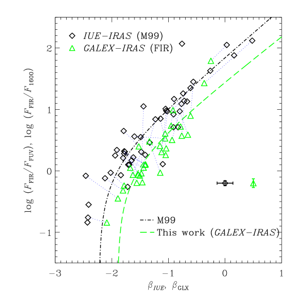
Figure 1: The IRX-$\beta$ relation obtained with GALEX and IRAS. Open squares represent the original data of (Meurer et al. 1999: M99), and filled circles are the new measurements from GALEX images in this work. A pair of symbols connected by dotted lines represents the same galaxy. Typical uncertainty for each measurement is indicated on the lower-left. For the original IUE measurements of M99, the abscissa is the UV slope of the IUE spectra of the sample $\beta$, and for the GALEX measurements, it is the slope defined by the UV color defined by the FUV and NUV photometry by GALEX [eq. (15)], $\beta_{\rm GLX}$ (Kong et al., 2004). As for the ordinate, it is the ratio between the FIR flux $F_{\rm FIR}$ [eq. (24)] and the 1600 Å flux $F_{1600}$ [eq. (3)], $F_{\rm FIR}/F_{1600}$ (referred to as the IRX) for the original M99 data, and the flux ratio between $F_{\rm FIR}$ and the GALEX FUV-band flux $F_{\rm FUV}$, $F_{\rm FIR}/F_{\rm FUV}$.

2.2 New measurement of UV flux by GALEX images

In order to examine the possible aperture effect of IUE, we remeasured the UV flux densities from GALEX images. As already mentioned, GALEX has two UV bands, FUV ($\lambda=1344\mbox{--}1786$ Å) and NUV ($\lambda=1771\mbox{--}2831$ Å). The GALEX images are available through MAST.

We have made a FUV and NUV photometry of the sample galaxies as follows:

1. Cut out a $30^{\prime}\times 30^{\prime}$ square subimage from GALEX AIS images around each galaxy

2. Select a subimage with the largest exposure time when multiple observations were available.

3. Measure FUV and NUV flux densities. The NUV image is taken as the reference.

In this study, it is important to mention that almost all of the sources are resolved by GALEX. Then, they very often appear as an assembly of small bright patchy regions, and the GALEX pipeline misidentifies these fragments as individual objects. This is referred to as shredding. We must deal with the shredding to obtain sensible flux density measurements for nearby extended galaxies. For this purpose, we have used an IDL software package developed by ourselves. This software performs aperture photometry in the NUV sub-image using a set of elliptical apertures. Total flux density is calculated within the aperture corresponding to the convergence of the growth curve. The sky background is measured by combining several individual regions around the source. NUV and FUV flux densities are corrected for Galactic extinction using the Schlegel map (Schlegel et al., 1998) and the Galactic extinction curve of Cardelli et al. (1989). A detailed description of the photometry process can be found in Iglesias-Páramo et al. (2006).

This was already used for previous studies (Iglesias-Páramo et al., 2006; Buat et al., 2007a; Takeuchi et al., 2010; Sakurai et al., 2011), and its performance is carefully checked and established. The new measurements are tabulated as $\log L_{\rm NUV}$ and $\log L_{\rm NUV}$ in Table 1.

Table 1: Sample of Meurer et al. (1999) with new measurements.

Name	$\beta$	$\beta_{\rm GLX}$	$\log L_{1600}$	$\log L_{\rm FUV}$	$\log L_{\rm NUV}$	$\log L_{\rm FIR}$	$\log L_{\rm TIR}$	Major axis	Minor axis	$z$	Type
			[$L_{\odot}$]	[$L_{\odot}$]	[$L_{\odot}$]	[$L_{\odot}$]	[$L_{\odot}$]	[arcsec]	[arcsec]
NGC4861	$-$2.46	$-$1.89	8.76	9.13	8.97	8.68	8.50	180.00	46.15	0.0028	SB
IZw18	$-$2.43	$-$2.09	…	8.05	7.86	…	…	31.50	14.70	0.0025	BCG
NGC1705	$-$2.42	$-$2.09	8.88	8.95	8.75	8.12	8.50	76.50	73.44	0.0021	SA0
Mrk153	$-$2.41	$-$1.78	9.20	9.38	9.24	8.65	…	27.00	18.69	0.0080	Scp
Tol1924$-$416	$-$2.12	$-$1.80	9.66	9.86	9.72	9.54	9.53	30.00	20.00	0.0095	pec
UGC9560	$-$2.02	$-$1.78	8.57	8.77	8.63	8.54	8.77	42.00	27.00	0.0039	pec
Mrk66	$-$1.94	$-$1.41	9.60	9.86	9.79	9.85	…	22.50	16.36	0.0210	BCG
NGC3991	$-$1.91	$-$1.67	9.68	9.96	9.84	10.02	10.11	61.50	28.38	0.0106	PEC
NGC3738	$-$1.89	$-$1.49	…	7.94	7.85	…	7.86	76.50	62.16	0.0008	Irr
UGCA410	…	…	…	…	…	…	…	…	…	0.0022	BCDG
Mrk357	$-$1.80	$-$1.44	10.66	10.81	10.73	10.87	11.03	25.50	19.83	0.0529	Pair
NGC3353	$-$1.79	$-$1.52	8.50	8.73	8.63	9.15	9.23	61.50	45.32	0.0031	Irr
MRK54	$-$1.78	$-$1.41	10.54	10.71	10.64	10.82	10.77	43.50	23.20	0.0449	Sc
NGC1140	$-$1.78	$-$1.51	9.07	9.46	9.37	9.39	9.72	81.00	47.03	0.0050	pec
Mrk36	$-$1.72	$-$1.32	7.75	8.47	8.41	7.49	8.40	150.00	28.68	0.0022	BCG
MCG6$-$28$-$44	$-$1.77	$-$1.40	10.51	10.71	10.64	10.82	10.77	43.50	23.20	0.0449	Sc
NGC1510	$-$1.71	$-$1.56	8.27	8.54	8.44	8.37	8.49	63.00	51.88	0.0030	SA0
MRK19	…	…	…	…	…	…	9.74	…	…	0.0138	Sa
NGC4214	$-$1.69	$-$1.56	…	9.01	8.91	…	9.05	337.50	225.00	0.0010	IAB
NGC4670	$-$1.65	$-$1.53	8.84	9.08	8.98	9.01	9.36	69.00	53.32	0.0036	SB0
NGC1800	$-$1.65	$-$1.63	…	8.62	8.51	…	8.31	67.50	35.10	0.0027	IB
UGC5720	$-$1.62	$-$1.42	8.93	9.05	8.97	9.15	9.66	34.50	31.85	0.0048	Im
UGC5408	$-$1.60	$-$1.06	8.98	9.01	9.00	9.54	9.78	34.50	26.83	0.0100	E/S0
NGC7673	$-$1.50	$-$1.27	…	9.98	9.93	…	10.41	51.00	45.00	0.0114	SAc
NGC3125	$-$1.49	$-$1.05	8.71	8.99	8.99	9.26	9.52	40.50	29.25	0.0037	BCdG
Haro15	$-$1.48	$-$1.63	9.96	10.33	10.22	10.27	10.44	52.50	43.24	0.0214	SB0
NGC2537	$-$1.44	$-$1.48	7.29	8.36	8.27	8.34	8.53	66.00	58.38	0.0014	SB(s)m
UGC3838	$-$1.41	$-$1.46	8.97	9.41	9.33	9.23	8.30	42.00	24.71	0.0102	Sd
NGC7793	$-$1.34	$-$1.58	…	8.94	8.84	…	9.08	354.00	200.26	0.0008	SA(s)d
NGC5253	$-$1.33	$-$1.18	…	8.95	8.92	…	9.26	123.00	69.62	0.0014	Im
NGC7250	$-$1.33	$-$1.14	8.71	9.20	9.17	9.17	9.34	49.50	19.04	0.0039	Sdm
Mrk542	$-$1.32	$-$0.99	…	9.64	9.64	…	10.27	27.00	23.14	0.0245	Im
NGC7714	$-$1.23	$-$1.34	9.54	9.90	9.84	10.38	10.48	40.50	24.92	0.0093	SB(s)
Mrk487	…	…	…	…	…	…	…	…	…	0.0022	BCDG
NGC3049	$-$1.14	$-$1.04	8.44	8.93	8.92	9.29	9.38	90.00	45.00	0.0049	SB(rs)
UGC6456	$-$1.10	$-$1.87	5.98	6.64	6.49	6.09	…	37.50	26.47	0.0003	pec
NGC3310	…	…	…	…	…	…	9.41	…	…	0.0033	SAB(r)
NGC5996	$-$1.04	$-$1.12	9.23	9.90	9.88	10.21	10.38	76.50	42.08	0.0110	SBc
NGC4385	$-$1.02	$-$1.06	8.85	9.20	9.19	9.82	10.01	73.50	36.75	0.0071	SB(rs)
Mrk499	$-$1.02	$-$0.82	…	9.88	9.92	…	10.35	31.50	27.56	0.0260	Im
NGC5860	$-$0.91	$-$0.78	9.32	9.51	9.55	10.24	10.38	43.50	35.59	0.0180	E/S0
IC1586	$-$0.91	$-$1.15	9.36	9.65	9.63	10.07	10.20	37.50	33.33	0.0194	BCG
NGC2782	$-$0.90	$-$0.95	9.12	9.55	9.56	10.29	10.49	82.50	61.21	0.0085	SAB(rs)
ESO383$-$44	…	…	…	…	…	…	10.12	…	…	0.0126	SA(s)
NGC5236	$-$0.83	$-$0.80	…	9.98	10.01	…	10.68	352.50	320.11	0.0017	SAB(s)
NGC2415	$-$0.80	$-$0.66	9.64	10.01	10.08	10.61	10.44	34.50	34.50	0.0126	Im
MCG$-$01$-$30$-$33	$-$0.77	$-$0.93	…	…	…	…	…	57.00	21.92	…00	SB(s)b
NGC1614	…	…	…	…	…	…	11.42	…	…	0.0159	SB(s)c
NGC6217	…	…	…	…	…	…	10.03	…	…	0.0045	SB(rs)
NGC6052	$-$0.72	$-$0.76	9.55	10.11	10.15	10.69	10.89	55.50	45.71	0.0158	Sc
NGC4500	…	…	…	…	…	…	10.37	…	…	0.0104	SB(s)a
IC214	$-$0.61	$-$0.92	9.83	10.18	10.20	11.18	11.30	43.50	31.90	0.0302	Irr
NGC3504	$-$0.56	$-$0.61	8.77	9.31	9.38	10.22	10.44	102.00	63.41	0.0051	SAB(s)
NGC4194	…	…	…	…	…	…	10.67	…	…	0.0083	BCG
NGC2798	0.03	$-$0.25	8.22	8.48	8.62	10.27	10.26	28.50	23.75	0.0058	SB(s)
NGC3256	…	…	…	…	…	…	11.29	…	…	0.0094	Pec
NGC7552	0.48	$-$0.37	8.66	9.35	9.47	10.78	10.78	111.00	62.83	0.0054	SB(s)

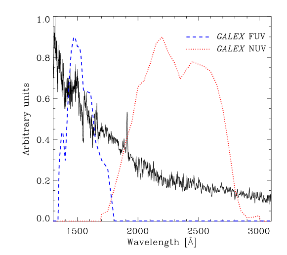
Figure 2: Example of IUE galaxy spectrum in Meurer et al. (1999) sample (NGC4861) with GALEX FUV and NUV filter response functions. Solid curve represents the observed spectrum of NGC4861 by IUE. Dashed and dotted lines are response functions of GALEX FUV and NUV filters, respectively. All are arbitrarily normalized.

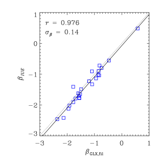
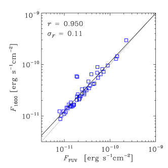
Figure 3: Comparison of the UV spectral slope $\beta$ and the 1600 Å flux density before and after transmitting the GALEX filters. Left: the $\beta$ derived by GALEX FUV and NUV photometry and that directly measured by IUE spectra; Right: the 1600 Å flux density through the GALEX FUV filter and that directly measured by IUE. Solid lines represent the linear fit to the data, and diagonal dotted lines in both panels show $y=x$.

3 Results

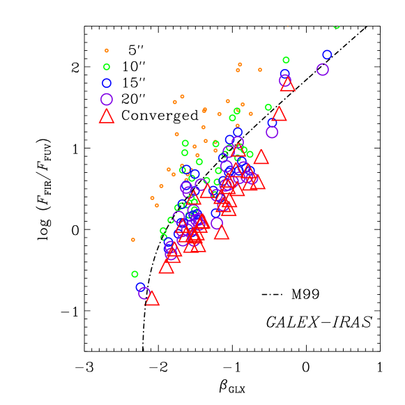
Figure 4: Behavior of the IRX-$\beta$ relation with the aperture radius on GALEXimages. The semi-major axis radius of the photometry ellipse is set to be $5^{\prime\prime}$, $10^{\prime\prime}$, $15^{\prime\prime}$, $20^{\prime\prime}$ from smaller to larger open circles. We also put the converged values of the growth curve of flux given by our software by open triangles.

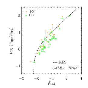
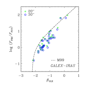
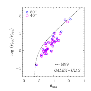
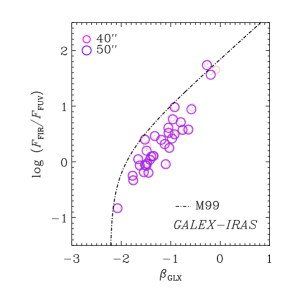
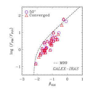
Figure 5: Effect of aperture size for the IRX-$\beta$ measurement. These figures are essentially the same as Fig. 4, but we show the change of the measured values with increasing aperture size with a step of $10^{\prime\prime}$ here. Upper-left: change of the IRX-$\beta$ relation with an aperture radius $10^{\prime\prime}\rightarrow 20^{\prime\prime}$; Upper-right: same but radius $20^{\prime\prime}\rightarrow 30^{\prime\prime}$; Middle-left: same but radius $30^{\prime\prime}\rightarrow 40^{\prime\prime}$; Middle-right: same but radius $40^{\prime\prime}\rightarrow 50^{\prime\prime}$; Lower: same but radius $50^{\prime\prime}\rightarrow\mbox{converged values}$.

3.1 Result with GALEX and IRAS

We show the result of new measurements for M99’s sample galaxies to examine the IRX-$\beta$ relation. We quantitatively define the slope of UV spectrum $\beta$ as the exponent of an approximated spectrum (in flux density per unit wavelength interval)

$$f_{\lambda}\propto\lambda^{\beta}\;.$$ (1)

The relation between the flux at wavelength $\lambda$, $F_{\lambda}$, and the flux density per unit wavelength interval at $\lambda$, $f_{\lambda}$ is

$$F_{\lambda}=\lambda f_{\lambda}=\nu f_{\nu}\;.$$ (2)

Thus the 1600 Å flux $F_{1600}$ is defined as the average flux around the central wavelength 1600 Å,

$$F_{1600}\equiv\lambda f_{\lambda}\mbox{@1600~{}\AA}\;.$$ (3)

The FIR flux $F_{\rm FIR}$ is defined by using flux densities $f_{\nu}$ at IRAS $60~{}\mu$m and $100~{}\mu$m as

$$F(60)=2.58\times 10^{-40}f_{\nu}(60~{}\mu\rm{m})\;,$$ (4)

$$F(100)=1.00\times 10^{-40}f_{\nu}(100~{}\mu\rm{m})\;,$$ (5)

$$F_{\rm FIR}=1.26[F(60)+F(100)]\;,$$ (6)

where the unit of $F(60)$, $F(100)$, and $F_{\rm FIR}$ is $[\rm{erg~{}s^{-1}~{}cm^{-2}}]$, and the unit of $f_{\nu}$ is $~{}[\rm{erg~{}s^{-1}~{}cm^{-2}~{}}~{}Hz^{-1}]$ (Helou et al., 1988). In this work, we denote the flux density per unit frequency interval at a wavelength $\lambda$ as $f_{\nu}(\lambda)$. We also use flux density in unit wavelength interval, $f_{\lambda}$. The unit of $f_{\lambda}$ is $\;[\mbox{erg}^{-1}\mbox{cm}^{-2}\mbox{s}^{-1}\mbox{\AA}^{-1}]$ throughout this paper. In M99, the IR and the UV fluxes were estimated from the IRAS and IUE data, respectively. Hence, we first use the original IRAS values of M99 for IR flux, and focus on the new UV measurements with GALEX. We should note that the FIR flux evaluated by eq. (4) is only the integrated flux over a wavelength range $42\mbox{--}122~{}\mu$m, and not the total IR flux often defined as integrated flux in a range $8\mbox{--}1000\;\mu\mbox{m}$. We evaluate the IR flux with AKARI later in Section 3.3.2.

With these observables and some empirical assumptions, M99 have formulated the relation between $\mbox{IRX}_{1600}$ and $A_{1600}$ as

$${\rm log(IRX_{1600})}={\rm log}(10^{0.4A_{1600}}-1)+\log B\;,$$ (7)

$$B\equiv\frac{\rm{BC(1600)_{*}}}{\rm BC(FIR)_{Dust}}=\mbox{const.}\;,$$ (8)

where BC stands for the bolometric correction. M99 adopted $\rm{BC}(1600)_{*}=1.66\pm 0.15$ for 1600 Å and BC(FIR)${}_{\rm Dust}=1.4\pm 0.2$ for IRAS FIR, which leads $B=1.19\pm 0.20$. We revisit this issue in Section 4.2. Thus, we obtain

$${\rm log(IRX_{1600})}={\rm log}(10^{0.4A_{1600}}-1)+0.076\pm 0.044\;.$$ (9)

The derivation of eqs. (7) and (9) is shown in Appendix A. Here, the value $B$ is for IUE and IRAS, and if we use different data, it will also change. Since we use GALEX FUV, we should recalculate $B$ for GALEX and IRAS. However, Seibert et al. (2005) obtained $\rm{BC}(\mbox{FUV})_{*}\simeq 1.68$, which is very close to that of IUE, yielding practically the same value for $B$. Assuming a linear relation between $A_{1600}$ and $\beta$ as

$$A_{1600}=a_{0}+a_{1}\beta\;,$$ (10)

namely the general relation between IRX and $\beta$ is expressed as

$$\log\left(\frac{F_{\rm FIR}}{F_{\rm FUV}}\right)=\log\left[10^{(0.4(a_{0}+a_{1}\beta)}-1\right]+0.076\;.$$ (11)

Performing a least square fit with observed values, M99 obtained a result

$$A_{1600}=4.43+1.99\beta\;.$$ (12)

Combining eqs. (12) with (11), we obtain

$$\log\left(\frac{F_{\rm FIR}}{F_{\rm FUV}}\right)=\log\left[10^{0.4(4.43+1.99\beta)}-1\right]+0.076\;.$$ (13)

This is the IRX-$\beta$ relation proposed by M99.

GALEX is a survey-oriented astronomical satellite, and its data are mainly images (though GALEX is also equipped with a spectrograph). Hence, we need to determine the UV spectral slope $\beta$ from FUV and NUV images, different from the case of IUE which is equipped with a spectrograph. Kong et al. (2004) proposed a method to estimate IRX and $\beta$ by using a flux density per unit wavelength $f_{\rm FUV}$ and $f_{\rm NUV}$ as follows.

$$\mathrm{IRX} \equiv \log\left(\frac{F_{\rm FIR}}{F_{\rm FUV}}\right)$$ (14)

$$\beta_{{\rm GLX}} \equiv \frac{\log f_{\rm FUV}-\log f_{\rm NUV}}{\log\lambda_{\rm FUV}-\log\lambda_{\rm NUV}}\;.$$ (15)

Here the effective wavelength of FUV and NUV bands are $\lambda_{\rm FUV}=1520$ Å and $\lambda_{\rm NUV}=2310$ Å, respectively.

The IRX-$\beta$ relation newly obtained by these quantities is shown in Fig. 1. We also show the original values of M99 for comparison. Same galaxies are connected with dotted lines in Fig. 1. The new values distribute clearly below the original ones of M99 for almost all galaxies. We found that since also the new values for $\beta$ are different, the distribution is shifted toward lower-right direction. Fitting eq. (11) to the new GALEX-IRAS IRX-$\beta$ measurements, we obtain

$$\log\left(\frac{F_{\rm FIR}}{F_{\rm FUV}}\right)=\log\left[10^{(0.4(3.45+1.82\beta)}-1\right]+0.076\;,$$ (16)

which is different from eq. (13) (see the dashed line in Fig. 1). The newly obtained relation is very close to that of normal star-forming galaxies proposed by previous studies (e.g., Buat et al., 2005; Cortese et al., 2006; Boissier et al., 2007; Takeuchi et al., 2010, , among others). This implies that the starbursts in M99 sample are hosted in a normal galaxies with redder colors. We will revisit this issue in Section 4.

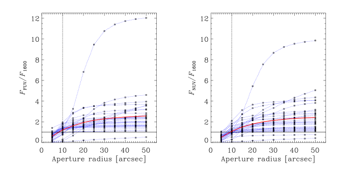
Figure 6: Behavior of GALEX FUV and NUV fluxes normalized by the IUE 1600 Å flux. Left: the flux ratio between GALEX FUV and IUE 1600 Å. Open squares connected by dotted lines represent the flux ratio for each sample galaxy as a function of the aperture radius. Solid thick curve is the average of all sample galaxies; Right: same as left panel but for GALEX NUV. A radius $10^{\prime\prime}$ is the semi-major axis radius of IUE aperture (see main text), which is indicated by vertical dotted lines in both panels.

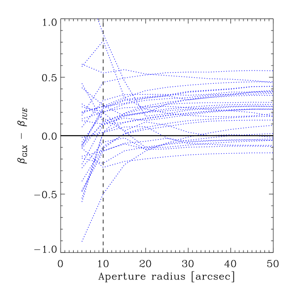
Figure 7: Behavior of the difference between $\beta_{{\rm GLX}}$ and $\beta_{IUE}$ as a function of aperture radius of our GALEX photometry. The slope from IUE, $\beta_{IUE}$ is fixed to the original M99 value for each sample galaxy. A radius $10^{\prime\prime}$ is the semi-major axis radius of IUE aperture (see main text), which is indicated by vertical dashed line. The horizontal solid line means $\beta_{\rm GLX}=\beta_{IUE}$. Again the radius $10^{\prime\prime}$ is indicated by vertical dashed line.

3.2 Examination of the result

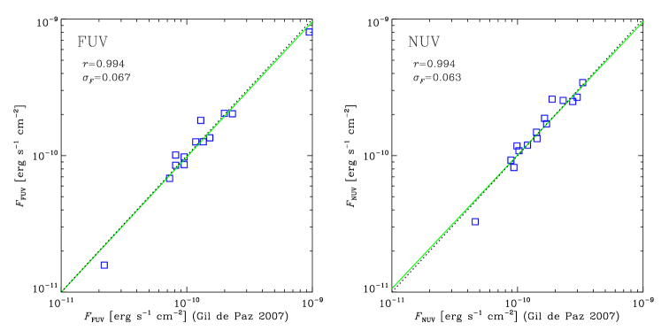
Figure 8: Comparison between the measurements of this work and that of Gil de Paz et al. (2007). Left panel shows the correlation of two measurements at FUV, and right panel is the same but at NUV. In both panels, open squares represent 11 galaxies commonly included both in the sample of Gil de Paz et al. (2007) and of this work. Solid lines represent the logarithmic linear fit to the sample. Dotted diagonal lines show $y=x$.

3.2.1 Effect of the filter response function of GALEX

As we mentioned above, GALEX data are basically images, then the photometric data would be affected by the filter response function. We should stress that the UV spectral slopes $\beta$ were obtained directly from the IUE spectrum, with avoiding the wavelength range corresponding to the 2170 Å bump (see e.g. Cardelli et al., 1989) of the Galactic extinction curve (Calzetti et al., 1994). In contrast, the GALEX NUV filter covers the bump. This would cause a systematic effect on the measurement of IRX and $\beta$. Since most of the high-$z$ galaxy surveys use photometric data to evaluate $\beta$ for applying the IRX-$\beta$ relation fort dust attenuation, it is crucial to calibrate the related quantities carefully. We first examine this effect.

For this, we convolve the response function with the IUE energy spectra of the M99 sample galaxies (see Fig. 2 as an example). Let $R_{\rm FUV}(\lambda)$ and $R_{\rm NUV}(\lambda)$ be the FUV and NUV filter response functions, respectively, and denote the raw IUE spectra as $f_{\lambda}$ and the flux density at FUV (NUV) as $f_{\rm FUV,fil}$ ($f_{\rm NUV,fil}$) $[\mbox{erg}^{-1}\mbox{s}^{-1}\mbox{cm}^{-2}\mbox{\AA}^{-1}]$, then we have

$$f_{\rm FUV,\rm{fil}} = \frac{\displaystyle\int_{\rm FUV}f_{\lambda}R_{\rm FUV}(\lambda)d\lambda}{\displaystyle\int_{\rm FUV}R_{\rm FUV}(\lambda)d\lambda}$$ (17)

$$f_{\rm NUV,\rm{fil}} = \frac{\displaystyle\int_{\rm NUV}f_{\lambda}R_{\rm NUV}(\lambda)d\lambda}{\displaystyle\int_{\rm NUV}R_{\rm NUV}(\lambda)d\lambda}\;.$$ (18)

With eqs. (17) and (18), IRX and $\beta$ after transmitting the GALEX filters, $\mbox{IRX}_{fil}$ and $\beta_{,\rm{fil}}$, are expressed as

$$\mathrm{IRX_{\rm{fil}}}=\log\left(\frac{F_{\rm FIR}}{F_{\rm FUV,\rm{fil}}}\right)$$ (19)

$$\beta_{{\rm GLX}_{\rm{fil}}}=\frac{\log f_{\rm FUV,\rm{fil}}-\log f_{\rm NUV,\rm{fil}}}{\log\lambda_{\rm FUV}-\log\lambda_{\rm NUV}}$$ (20)

$$F_{\rm FUV,\rm{fil}}=\lambda_{\rm FUV}f_{\rm FUV,\rm{fil}}\;.$$ (21)

We show the comparison of the UV spectral slope $\beta$ and the 1600 Å flux densityGALEX before and after transmitting the GALEX filter in Fig. 3. For this analysis, we restricted to galaxies only with spectra in the full range of IUE wavelength coverage ($1100\mbox{--}3000$ Å). In the M99 sample, there are samples only with spectra at IUE SW spectral coverage, and they are not ideal for the purpose of this analysis here. As we see in the left panel of Fig. 3, $\beta$ directly measured by IUE and that defined by GALEX show a very good agreement. The linear fit gives

$$\beta_{{\it IUE}}=1.01\beta_{{\rm GLX,fil}}-0.07$$ (22)

with the Pearson’s correlation coefficient of $r=0.976$ and the standard deviation is $\sigma_{\beta}\simeq 0.14$. The systematic deviation is smaller than $\sigma_{\beta}$. As for the flux density, as we see on the right panel in Fig. 3, the 1600 Å flux density measured by IUE, $F_{1600}$, tends to be about 10 % larger than that transmitted through the GALEX FUV filter, $F_{\rm FUV,fil}$. The logarithmic linear fit yields

$$\log F_{1600}=0.949\log F_{\rm FUV,fil}-0.462$$ (23)

with the Pearson’s correlation coefficient of $r=0.950$ and the standard deviation of flux density $\sigma_{F}\simeq 0.11$ in logarithmic scale. Again, the systematic deviation is smaller than $\sigma_{F}$. Considering the intrinsic scatter in the IRX-$\beta$ plot in M99, we can safely neglect the systematic differences in $\beta$ and $F_{\rm FUV\;or\;NUV}$ in the following analysis.

3.2.2 Effect of the aperture size

In order to examine the effect of aperture photometry on GALEX images, we observe the behavior of flux with varying the aperture size. In this work, the aperture radius $\theta^{\prime\prime}$ of the photometry is defined as an ellipse with semi-major axis size $\theta^{\prime\prime}$. This ellipse is determined automatically by fitting to the isophotal ellipse of a galaxy by our photometry software. Then, the flux within a radius of $10^{\prime\prime}$ means the integrated flux in an ellipse with semi-major axis size of $10^{\prime\prime}$. Figure 4 shows the change of measured values on the IRX–$\beta$ plot when we change the GALEX aperture radius as $5^{\prime\prime}$, $10^{\prime\prime}$, $15^{\prime\prime}$, $20^{\prime\prime}$, and the convergence radius (depends on the sample). To see the change more clearly, we also show the change of the measured values with increasing aperture size with a step of $10^{\prime\prime}$ in Fig. 5.

In Fig. 6, we compare GALEX FUV and NUV flux densities and IUE $F1600$ flux. Here, the circle-equivalent “effective” IUE aperture of $14^{\prime\prime}$ is shown as vertical lines. This is an approximate of the IUE aperture size which was an ellipse of $10^{\prime\prime}\times 20^{\prime\prime}$. We set the ellipse shape and position angle to be the same as that used in actual IUE observation of the sample galaxies. This IUE effective aperture is depicted by vertical lines in both panels of Fig. 6. As shown in this figure, FUV fluxes do not start to converge around a radius of $10^{\prime\prime}$–$20^{\prime\prime}$ but continue to increase, and finally converge to values approximately 2.5 times larger than the 1600 Å fluxes. The NUV flux also show a similar behavior to that of FUV. We should also note that the behavior of FUV and NUV growth curves is not exactly the same. This causes an aperture dependence of $\beta$.

To see this effect, we examined the difference of $\beta$ between IUE and GALEX. Figure 7 depicts the behavior of $\beta_{\rm GLX}-\beta_{IUE}$ as a function of aperture radius. We observe that the behavior of $\beta$ is not monotonic: some increase and others decrease after exceeding $14^{\prime\prime}$ aperture, and finally start to converge to certain values at much larger radius. Within the effective IUE aperture radius, $\beta_{{\rm GLX}}$ changes significantly for most of the sample and is still far from the convergence values. We see a weak tendency that the converged values of $\beta$ are larger than that listed in M99, i.e., the global UV color of the sample turned out to be slightly redder when we measure the integrated flux. This can be explained as follows: since the M99 sample consists of central starbursts, it may be natural that their outer part of the disk has redder colors than the central part. Hence, the colors of central part are bluer than the global ones. Thus, the values of $\beta$ determined at a radius similar to that of IUE are systematically bluer than the UV slopes when larger apertures are used.

We, therefore, conclude that the systematic deviation of the IRX-$\beta$ relation from the original one is due to the effect of UV flux because of the small IUE aperture. Especially, we see there is a galaxy that shows a very prominent behavior in Fig. 6. Both at FUV and NUV, this galaxy converges to exceptional values much brighter than the fluxes at a radius of $10^{\prime\prime}$. This galaxy is NGC 2537, which has very strong contribution of UV flux from the peripheral regions. Because of this, for NGC 2537, the IUE flux is more than an order of magnitude underestimated.

3.2.3 Verification of the result with Gil de Paz et al. (2007)

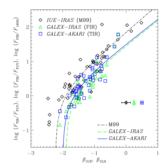
Figure 9: New IRX-$\beta$ relation obtained by GALEX and AKARI diffuse map. Measurements with IUE-IRAS, GALEX-IRAS, and GALEX-AKARI are plotted. Diamonds, triangles, and squares represent the IUE-IRAS, GALEX-IRAS, and GALEX-AKARI values. Dot-dashed curve represents the original M99 formula [eq. (13)], dashed curve for GALEX -IRAS fit [eq. (16)], and solid curve for the new formula with GALEX-AKARI measurements [eq. (30)]. Note that for IUE-IRAS and GALEX-IRAS, the IR flux is evaluated by FIR (Helou et al., 1988), while for GALEX-AKARI it is evaluated by total IR emission (TIR: Takeuchi et al., 2010).

In the previous sections, we have shown that the UV flux measurement of M99 was significantly underestimated because of the small aperture size of IUE. However, since the photometry software we used for this work has been developed originally by ourselves (cf. Iglesias-Páramo et al., 2006), we should examine if there would be any systematic effect caused by the difference in photometry softwares when we compare our results with other ones.

Gil de Paz et al. (2007) also used original software to perform a photometry of GALEX images. We checked the sample of Gil de Paz et al. (2007) and found 18 galaxies common with M99, among which we have 11 galaxies with measurements needed for this study (Gil de Paz et al., 2007, see their Table 4).

Figure 8 shows that the results of this work and that of Gil de Paz et al. (2007) agree with each other very well. The correlation coefficient and the standard deviation for FUV data are $r=0.994$ and $\sigma_{F}({\rm FUV})=0.0670$ in logarithmic scale, and the same for NUV data are $r=0.994$ and $\sigma_{F}({\rm NUV})=0.0630$, respectively. Thus, we can safely conclude that both measurements are in excellent agreement. This means that the aperture effect on the original IRX-$\beta$ relation was independently proved by Gil de Paz et al. (2007). Now we can safely conclude that the reason of the systematic shift of the IRX-$\beta$ relation of recent studies and the original one is dominantly caused by the small aperture of IUE. Now we have the GALEX-IRAS based IRX-$\beta$ relation which is free from the aperture effect [eq. (16)].

3.3 New IRX-$\beta$ relation with GALEX and AKARI

Up to now, we concentrated on the examination of UV flux measurement for the IRX-$\beta$ relation, and for this purpose we kept the M99’s original values $F_{\rm FIR}$ from IRAS. Here we discuss the IR flux.

3.3.1 Total IR flux by AKARI

The M99 relation was constructed to relate the UV slope and IRX $(F_{\rm FIR}/F_{\rm 1600})$, and they used the FIR luminosity (Helou et al., 1988)

$$L_{\rm FIR}\equiv 3.29\times 10^{-22}\times\left[2.58L_{\nu}(60\;\mu\mbox{m})+L_{\nu}(100\;\mu\mbox{m})\right]\;[\rm{L}_{\odot}]\;.$$ (24)

However, as mentioned above, $L_{\rm FIR}$ contains only the luminosity in a wavelength range of $\lambda=42-122~{}\mu$m, and energy emitted at MIR ($5\mbox{--}30~{}\mu$m) nor submillimeter ($300\mbox{--}1000~{}\mu$m) is not considered. Hence, the FIR luminosity is proved to be a significant underestimation as a representative of the total IR luminosity ($L_{\rm TIR}$) (e.g., Takeuchi et al., 2005b). Dale et al. (2001) and Dale & Helou (2002) proposed formulae to convert FIR into TIR luminosity by making use of IRAS flux densities.

The AKARI FIS All-Sky Survey data are publicly available. With AKARI fluxes, Takeuchi et al. (2010) proposed a new simple formula to estimate $L_{\rm TIR}$ precisely as follows

$$\Delta\nu(\mbox{\it WIDE-S\,})=1.47\times 10^{12}~{}[\rm{Hz}]\;,$$ (25)

$$\Delta\nu(\mbox{\it WIDE-L\,})=0.831\times 10^{12}~{}[\rm{Hz}]\;,$$ (26)

$$\log L_{\it AKARI}^{2\rm{band}}=\Delta\nu(\mbox{\it WIDE-S\,})L_{\nu}(90~{}\mu\mbox{m})\;,$$

$$\qquad\qquad\qquad+\Delta\nu(\mbox{\it WIDE-L\,})L_{\nu}(140~{}\mu\mbox{m})$$ (27)

$$\log L_{\rm TIR}=0.964\log L_{\it AKARI}^{2\rm{band}}+0.814\;.$$ (28)

Here $\Delta\nu$ is the bandwidth of each AKARI FIS filter expressed in units of frequency (Hirashita et al., 2008).

3.3.2 New IRX-$\beta$ relation with GALEX and AKARI

Combining the GALEX-based UV flux free from the IUE aperture effect and the AKARI TIR flux [eq. (28)] covering the whole IR wavelength range, we construct a new IRX-$\beta$ relation applicable for recent studies with AKARI, Spitzer, and Herschel.

We cross-matched the M99 sample with the database of AKARI FIS BSC. Among the M99 sample, 48 are detected by AKARI FIS. Among these 48 galaxies, 40 have GALEX FUV and NUV (see Table 1). With these 40 subsample galaxies of M99, we estimated the new IRX-$\beta$ relation.

Again the UV slope of the SED, $\beta$, was obtained by eq. (15), and the IRX was estimated from GALEX FUV flux and AKARI TIR flux as follows.

$$\mathrm{IRX} = \log\left(\frac{F_{\rm TIR}}{F_{\rm FUV}}\right)\;.$$ (29)

The result is presented in Fig. 9. Since the IRAS FIR is only a part of the AKARI TIR, the GALEX-IRAS values distribute in a lower region than the GALEX-AKARI measurements on the IRX-$\beta$ plots.

However, we should carefully check one issue here. Since we tried to be careful about the aperture effect at UV, we should also examine if the AKARI BSC fluxes are not affected by the aperture effect. Importantly, Yuan et al. (2011) examined a sample of Local galaxies extracted from that of Takeuchi et al. (2010), since they are mostly nearby resolved galaxies by using AKARI diffuse map. They remeasured the IR fluxes with AKARI diffuse images and found that the flux of extended galaxies tends to be underestimated in the AKARI FISBSC, which adopted a complicated point source extraction procedure. Then, according to Yuan et al. (2011), we measured the M99 sample with AKARI FIS diffuse map and compared the obtained flux with that in the FISBSC (Appendix B). Since M99 tried to remove very extended galaxies in the primary construction of the sample, the current sample was found to be less affected by this effect, but still for some galaxies the underestimation was significant. We thus used the fluxes from the AKARI diffuse map and used them for the final determination of the IRX-$\beta$ relation. This is shown in Fig. 9.

For fitting eq. (11) to the data, we should recall that this is a formula constructed for IRAS measurement, reflected in the term $\log B$. Since the bolometric correction for TIR, BC(TIR) is unity by definition, the last constant term in eq. (11) [i.e., eq. (A10)] simplifies to the logarithm of the bolometric correction at UV, $\log\mbox{BC(FUV)}_{*}\simeq 0.22$. Fitting the eq. (11) to the GALEX-AKARI data with this modification yields the following formula.

$$\log\left(\frac{L_{\rm TIR}}{L_{\rm FUV}}\right)=\log\left[10^{0.4(3.06+1.58\beta)}-1\right]+0.22\;.$$ (30)

This is the new unbiased IRX-$\beta$ relation for UV-selected starburst galaxies free from any aperture effect in UV or IR, applicable for present-day observational datasets with UV images (like GALEX) and total integrated IR flux (like that obtained by AKARI).

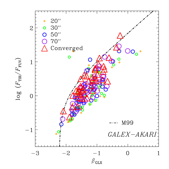
Figure 10: The IRX-$\beta$ diagram as a function of the aperture size both on GALEX and AKARI images. The same elliptical apertures were applied to both of the images. To address the difference of the angular resolutions of GALEX and AKARI, we have convolved the GALEX FUV images with the synthesized PSF of AKARI FIS 140 $\mu$m band. Since AKARI angular resolution is $\sim 50^{\prime\prime}$ at longer wavelenghts, photometric values with aperture radii smaller than $20^{\prime\prime}$ are not shown. Note that the aperture radii are different from that in Fig. 4: they are $20^{\prime\prime}$, $30^{\prime\prime}$, $50^{\prime\prime}$, and $70^{\prime\prime}$.

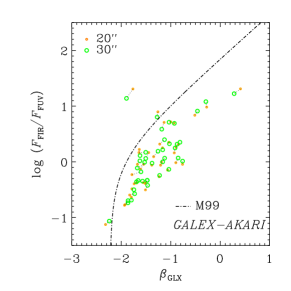
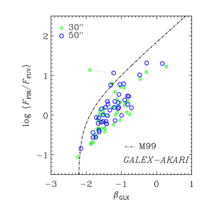
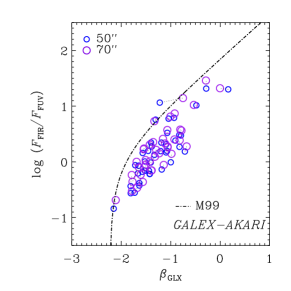
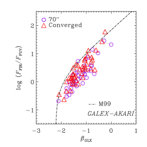
Figure 11: Similar to Fig. 5 but with varying aperture size both on GALEX and AKARI images. The GALEX FUV images are again convolved with the synthesized PSF. Since AKARI angular resolution is $\sim 50^{\prime\prime}$ at longer wavelenghts, we start the aperture radius from $20^{\prime\prime}$.

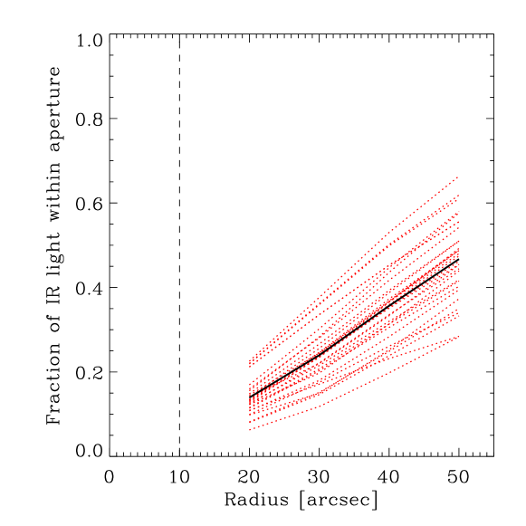
Figure 12: The fraction of the total IR light within an aperture radius. Dotted lines are the measured fraction for each sample galaxy, and the thick broken solid line shows their average. Vertical dashed line represent the semi-major axis of IUE elliptical aperture. The leak of flux to the sidelobes of the AKARI PSF is not corrected, but this does not change the conclusion significantly.

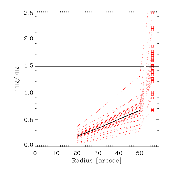
Figure 13: The ratio between TIR and FIR as a function of the aperture radius. Since FIR values are measured from IRAS, we fix them and measured the TIR/FIR ($F_{\rm TIR}/F_{\rm FIR}$) ratio as a function of aperture radii on AKARI images. Dotted lines represent the TIR/FIR ratio as a function of aperture radius, and the symbols represent convergence values of TIR/FIR for each sample. The thick solid broken line shows the average value. The horizontal thick line shows the convergence value of TIR/FIR at large aperture limit. Correspondence between the data values at $50^{\prime\prime}$ radius and convergence values is indicated also by the dotted lines, with a vertical gap to clarify that there is a large radius range omitted between them. The leak of flux to the sidelobes of the AKARI PSF is again not corrected.

4 Discussion

4.1 IRX as a function of aperture radius

In the above discussion, we have rather focused on the aperture effect of the UV photometry on the IRX-$\beta$ relation. Since we have the AKARI diffuse image map, it would be also interesting to explore the radial dependence of the IRX values. Here we estimate the IRX-$\beta$ relation as a function of aperture radius both on the GALEX and AKARI images. For this purpose, we have put the same elliptical aperture homologous to the original IUE one, both on these images for each galaxy.

Since the angular resolution of the AKARI diffuse image map is $\sim 30\mbox{--}50^{\prime\prime}$ at WIDE-S band, smaller aperture radii than $20^{\prime\prime}$ are not meaningful. We started an aperture radius from $20^{\prime\prime}$ which is similar to the IUE aperture radius, and then estimated the IRX with $30^{\prime\prime}$, $50^{\prime\prime}$, and $70^{\prime\prime}$ radii. We should also take into account the different of the PSFs at FIR and FUV. It is pointed out that the synthesized PSFs of the AKARI diffuse map are more extended than the previous estimates, with a significant flux leak to the sidelobes (Arimatsu et al., in preparation). Since it is still difficult to evaluate this effect precisely at this moment, we instead convolved the GALEX FUV images with the difference of the angular resolutions of GALEX and AKARI, we have convolved the GALEX FUV images with the synthesized PSF of AKARI FIS 140 $\mu$m band and measured the IRX within the same aperture at FIR and FUV bands. The result is shown in Figs. 10 and 11.

It is very clearly seen that the IRX values of central regions of the sample are much lower than the relation obtained from the whole galaxies. This is mainly because of the difference of the surface brightness profiles at FUV and FIR wavelengths. In general, the FUV light of galaxies is much more concentrated than that of FIR. Then, the IRX values are well below the convergence values within $15^{\prime\prime}$ aperture, and then moves up the diagram with increasing aperture radius, as clearly seen in Fig. 11. Even with the $50^{\prime\prime}$ aperture radius, the IRX values are still far from the convergence values for some galaxies, even if we take into account the difference of the PSFs. This implies that the starburst regions of the M99’s original sample galaxies emit less energy at FIR compared to the whole galaxy scale.

To see this more clearly, we show the fraction of TIR flux as a function of aperture radius in Fig. 12. Though the values are largely dispersed, on average the fraction contained in $20^{\prime\prime}$ aperture radius is $8.8\pm 3.1$ %. Namely, though we should keep in mind that the correction factor of the flux leak could be large at small aperture radii, at least we can claim that less than $\mbox{a few}\times 10$ % of the TIR light is associated to the central starburst regions in the sample, but comes from outer part of galaxies.

It will be interesting to simulate the IRX as a function of redshift, taking into account a realistic beam size and detection limit for current/future observational facilities to interpret the high-$z$ IRX-$\beta$ relation.

4.2 Bolometric correction for the total dust emission

Since the original IRX-$\beta$ relation was based on IRAS observation, we should convert the formula to that of TIR and FUV. The assumption of M99 was, as stated above, the ratio of TIR/FIR [the bolometric correction of dust emission, $\rm BC(FIR)_{Dust}$: see eq. (7)] is $\sim 1.4$. Many authors used this value to rescale the relation with this factor to obtain the IRX defined by $\log\left(F_{\rm TIR}/F_{\rm FUV}\right)$ (e.g. Kong et al., 2004). Then, it is important to examine the value of $\rm BC(FIR)_{D}ust$ by new IR data.

By making use of the AKARI FIS diffuse map, we examine the ratio of TIR and IRAS-based FIR. We calculated a ratio of TIR/FIR ($F_{\rm TIR}/F_{\rm FIR}$), shown in Fig. 13. In Fig. 13, the TIR/FIRs among the sample galaxies and its convergence values are presented. In Fig. 13, dotted lines represent the TIR/FIR ratio, and the symbols represent convergence values of TIR/FIR for each sample. The thick solid broken line shows the average value. The horizontal thick line shows the convergence value of TIR/FIR at large aperture limit. From this analysis, we found that the TIR/FIR ratio converges to $1.44\pm 0.574$, which is very close to the ratio originally assumed by M99. By using a formula of Dale & Helou (2002), Kong et al. (2004) discussed that TIR/FIR is $\sim 1.5$, which is also quite close to our value.

4.3 Comparison of IRX-$\beta$ relations between various samples

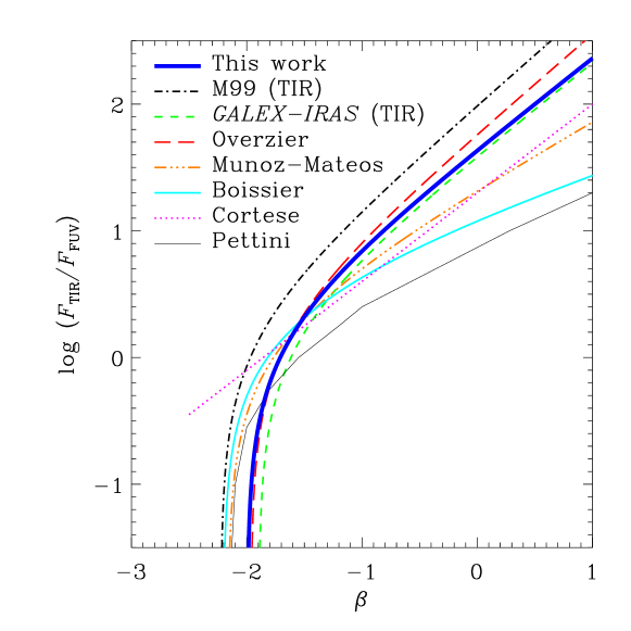
Figure 14: Comparison of various IRX-$\beta$ relations in the literature. Thick solid curve: this work; dot-dashed curve: M99’s curve converted from $F_{\rm FIR}/F_{1600}$ to $F_{\rm TIR}/F_{1600}$; dashed curve: curve for the M99’s sample but with new measurements at UV and converted for IR flux, i.e., $F_{\rm TIR}/F_{\rm FUV}$. long dashed curve: same as $F_{\rm TIR}/F_{\rm FUV}$ but with measurements by Overzier et al. (2011); three-dot-dashed curve: the IRX-$\beta$ relation for optically selected sample (Muñoz-Mateos et al., 2009); solid curve: similar to Muñoz-Mateos et al. (2009) but with older data (Boissier et al., 2007); dotted curve: a (bisector) linear fit by Cortese et al. (2006); and thin broken solid curve: the IRX-$\beta$ relation from the SMC extinction curve (Pettini et al., 1998).

We now compare our new formula with previous studies on the IRX-$\beta$ relation with various sample selection. We summarize the comparison in Fig. 14. Cortese et al. (2006) compiled a sample of optically selected galaxies observed by GALEX and analyzed the IRX-$\beta$ relation, as well as the IUE-selected UV starbursts. They have converted the FIR flux to the TIR one by the formula of Dale et al. (2001). Since the formula of Dale et al. (2001) is defined for a wavelength range of $\lambda=3\mbox{--}1000\;\mu$m, it gives a slightly larger value than our formula, but the difference is small enough compared with the intrinsic scatter and measurement errors (Takeuchi et al., 2005b). To describe the average trend, they fit a simple linear function instead of the form of eq. (11). In their analysis, Cortese et al. (2006) found that the optically selected sample distribute systematically lower than starbursts on the IRX-$\beta$ plane. They suggested qualitatively that this is partially due to the IUE aperture, as well as some physical reason related to the star formation activity. Our formula passes through the peak of the distribution of their optical sample, and agrees very well with their linear fit at $\beta\gtrsim-1$.

Boissier et al. (2007) selected 43 nearby late-type spiral galaxies optically and performed a detailed analysis on the dust attenuation. The sample was cross-matched with GALEX Atlas of Nearby Galaxies (Gil de Paz et al., 2007) for UV and IRAS HIRES images for IR. The same as Cortese et al. (2006), Boissier et al. (2007) also used the formula of Dale et al. (2001) to compute the TIR flux from IRAS flux. For the fitting of the IRX-$\beta$ relation, they used a form

$$\log\left(\frac{F_{\rm TIR}}{F_{\rm FUV}}\right)=\log\left[10^{a_{0}+a_{1}({\rm FUV}-{\rm NUV})}-a_{2}\right]\;,$$ (31)

which has one more free parameter than eq. (30). Their sample also distributed below the M99 relation (their Fig. 1). Their IRX-$\beta$ relation has a higher IRX at smaller $\beta$ and lower IRX at larger $\beta$, but since there are very few or no data at $\beta<-2$, the discrepancy on this side is not crucial. At the larger $\beta$ side, actually there is a large dispersion in optically selected spiral galaxy sample in Boissier et al. (2007). This may be the reason of their flat slope. Indeed, Muñoz-Mateos et al. (2009) used the SINGS galaxy sample (Kennicutt et al., 2003) for a similar analysis and obtained an IRX-$\beta$ relation with steeper slope at large $\beta$ side. The new relation of Muñoz-Mateos et al. (2009) is in a very good agreement with our result at $\beta>-1.5$. Thus, we can safely say that our new IRX-$\beta$ formula determined by the original UV starburst sample of M99, also describes the attenuation of optical sample very well. However, we should keep in mind that there is a considerable scatter around the relation obtained by fitting, as these authors also cautioned.

Next, we also examine if eq. (30) would apply to the IR-selected samples. As we have already seen, the behavior of IR-selected galaxies on the IRX-$\beta$ plane is quite complicated. These galaxies have two branches of distribution, one locates below the M99 relation and the other spreads well above the line (e.g., Buat et al., 2005, 2010; Takeuchi et al., 2010).

Goldader et al. (2002) first discovered that the population distributing above the M99 line is LIRGs or ULIRGs. Takeuchi et al. (2010) examined this aspect intensively and found that the population distributing lower than the M99 line is quiescent star-forming galaxies, and confirmed that the one above the M99 line is LIRGs or ULIRGs, by evaluating the 60-$\mu$m luminosity of AKARI FISBSC sample.

Buat et al. (2005) presented an impressive IRX-$\beta$ plots for both GALEX NUV- and IRAS 60 $\mu$m-selected samples. The quiescent branch of IR-selected galaxies distribute in almost the same way as the UV-selected sample on this plane, i.e., below the M99’s IRX-$\beta$ relation but in parallel with it. More active branch galaxies are spread over the M99 relation. We see that the former is well described by eq. (30) without significant bias. However, since the distribution of (U)LIRGs are very different from that of quiescent galaxies, our new relation cannot apply to these active galaxies.

As for high-$z$ galaxies, still it is not very easy to obtain both UV and IR data, but gradually direct measurements are reported recently. Siana et al. (2009) showed the IRX-$\beta$ measurements for two such objects, MS1512-cB58 ($z=2.724$) and the Cosmic Eye ($z=3.074$), both of which are Lyman-break galaxies (LBGs), i.e., UV-luminous starbursts. They found that they locate significantly below the original M99 relation. Reddy et al. (2010) also discussed the IRX-$\beta$ relation for both UV- and IR-luminous galaxies at $z\sim 2$. They found that their “typical” $z\sim 2$ galaxies do follow the M99 relation (but with a large scatter), and ULIRGs at the same redshift locate well above it similarly to their Local counterparts. Also they argue that young galaxies at these redshifts distribute below the M99 line. The young galaxies seem to follow the IRX-$\beta$ relation expected for the SMC extinction curve (Pettini et al., 1998), also suggested by Siana et al. (2009). Comparing their results with our new IRX-$\beta$ relation (see Fig. 14), we would say the $z\sim 2$ typical galaxies of Reddy et al. (2010) locate above the new IRX-$\beta$ relation, while the young galaxies follow it. As for lensed $z\sim 3$ galaxies in Siana et al. (2009), cB58 is approximately on the new relation, while the Cosmic Eye may be still below the relation. It would be very interesting to make a statistical analysis when a large sample of galaxies at these redshifts will be available, to discuss whether evolutionary effect really would take place. We should note that the IRX-$\beta$ relation of the central starburst regions of our sample locates well below the M99’s original relation and our new result, but more similar to the Pettini’s relation (see top-left panel of Fig. 11). Since M99 originally selected the sample to have a central starbursts, we might speculate, for example, that the properties of high-$z$ star-forming galaxies could be similar to that of a pure starburst region. Further investigation in this direction will be interesting.

Kong et al. (2004) suggested a systematic sequence of the IRX-$\beta$ relation from lower to higher along with the birthrate parameter $b$

$$b\equiv\frac{\mbox{SFR}(t_{0})}{\langle\mbox{SFR}\rangle}$$ (32)

where $t_{0}$ is a supposed age of a galaxy (Kennicutt et al., 1994). They claimed that $b$ is related to the attenuation as

$$A_{\rm FUV}=3.87+1.87(\beta_{\rm GLX}+0.40\log b)\;.$$ (33)

In Kong et al. (2004), the original M99 relation corresponds to the extremely bursting group, i.e., $b>3.0$, not very consistent with the properties of M99’s UV-luminous starburst sample. We see that our new IRX-$\beta$ relation corresponds to the intermediate $b$ galaxies similar to normally star forming galaxies, now consistent with the original M99 sample.

Overzier et al. (2011) independently made essentially the same analysis with this study but with their own GALEX photometry and IRAS-based IR flux estimation with a conversion formula of Dale et al. (2001), with Spitzer measurement for a subsample of 12 galaxies Their formula is, as we expect, not very different from our result [eq. (30)], but slightly deviated upward than ours at large $\beta$ and high IRX regime. They have measured the UV flux up to $2.5\mbox{--}5$ times Kron radius of galaxies, their converged values are on average twice larger than the original values of M99. As we have shown, the IUE flux is underestimated with a factor of 2.5 on average, and sometimes the underestimation is of an order of magnitude. Hence, though they discuss that the quiescent IR galaxies in Buat et al. (2010) locate lower than their line, for example, this might be due to the UV flux still missed.

5 Conclusion

The relation between the ratio of infrared (IR) and ultraviolet (UV) flux densities (the infrared excess: IRX) and the slope of the UV spectrum ($\beta$) of galaxies plays a fundamental role in the evaluation of the dust attenuation of star forming galaxies especially at high redshifts. M99 first introduced a very useful method to estimate the dust attenuation by using the relation between the FIR-to-FUV flux ratio and the UV slope, the IRX-$\beta$ relation. However, subsequent studies revealed a dispersion and/or systematic deviation from the original IRX-$\beta$ relation of M99, depending on sample selection. We reexamined the original IRX-$\beta$ relation proposed by M99 by measuring the far- and near-UV flux densities of the original sample galaxies used by M99 with GALEX imaging data. We summarize our conclusion as follows:

1. The UV flux densities of the galaxies used in M99 were significantly underestimated because of the small aperture of IUE which was $10^{\prime\prime}\times 20^{\prime\prime}$. Consequently, the IRX values were lower than that in M99, which lead the IRX-$\beta$ relation shifted downward on the plot.

2. The aperture effect affected not only the IRX but also $\beta$, because the curve of growth of the flux densities is a function of aperture which depends strongly on the wavelength.

3. Correcting the aperture effect, we obtained a new IRX-$\beta$ relation for UV-selected starburst galaxies for the same sample with M99.

4. The original relation was obtained based on IRAS data. Since IRAS bands cover only a wavelength range of $\lambda=42\mbox{--}122\;\mu$m, the FIR flux calculated from IRAS flux does not represent the total IR emission from dust. We used data from AKARI  which has a much wider wavelength coverage especially toward longer wavelengths, and obtained an appropriate IRX-$\beta$ relation for the data with total dust emission.

5. We also estimated the IRX-$\beta$ relation of the sample as a function both on the GALEX and AKARI images. We found that the IRX-$\beta$ relation of the central starburst regions of the sample locates significantly below the relation obtained for the whole galaxy regions. This means that the extended dust emission is important to evaluate various global properties of galaxies, though we need to know the behavior of the PSFs of AKARI diffuse map more precisely to evaluate more quantitatively.

6. In many previous studies, authors use a conventional conversion factor (bolometric correction: BC) of $\sim 1.4$ to obtain the total IR flux from dust. We examined the BC of dust emission and found that indeed the value was $1.44\pm 0.574$ on average.

7. Our new relation is consistent with most of the preceding results on the IRX-$\beta$ relation for samples selected at optical and UV, though there is a significant scatter around it. We also found that even the quiescent class of IR galaxies follow this new relation, though luminous and ultraluminous IR galaxies distribute completely differently.

8. The IRX-$\beta$ relation for the central starburst regions of M99’s sample galaxies is very similar to the relation proposed by Pettini et al. (1998), based on the SMC attenuation curve. This may imply interesting property of high-$z$ star-forming galaxies.

In this work, we constructed a proper formula for a category of galaxies which are luminous in UV and actively forming stars. We found that this formula also applies to various class of moderately star-forming galaxies, like optically selected or non-luminous IR selected ones. This will be a more firm basis than before when one needs to correct dust extinction of high-$z$ galaxies. However, we should note the large intrinsic scatter on the IRX-$\beta$ plane, especially the (U)LIRG population which does not obey the IRX-$\beta$ relation at all. Many issues and problems still remain to be solved for understanding this relation.

First of all, we thank the anonymous referee for her/his extremely careful and constructive comments and suggestions that improved this article significantly. This work is based on observations with AKARI, a JAXA project with the participation of ESA. We thank Yasuo Doi for preparing the AKARI FIS diffuse map for our sample galaxies, and Ko Arimatsu for providing the new synthesized PSF of the map. We also thank Véronique Buat, Denis Burgarella, Agnieszka Pollo, Ryosuke Asano, Fumiko Nagaya, Mai Fujiwara, Daisuke Yamasawa, and Takashi Kozasa for fruitful discussions and comments. We are grateful to Takako T. Ishii for developing the basis of the photometric software with IDL. TTT has been supported by Program for Improvement of Research Environment for Young Researchers from Special Coordination Funds for Promoting Science and Technology. TTT and AKI have been also supported by the Grant-in-Aid for the Scientific Research Fund (20740105, 23340046, 24111707: TTT, 19740108: AKI) commissioned by the Ministry of Education, Culture, Sports, Science and Technology (MEXT) of Japan. TTT, FTY, AI, and KLM have been partially supported from the Grand-in-Aid for the Global COE Program “Quest for Fundamental Principles in the Universe: from Particles to the Solar System and the Cosmos” from the MEXT.

Facilities: GALEX, IUE, IRAS, AKARI

Appendix A A. Formulation of Meurer et al. (1999)

Here, we review the original formulation of the IRX-$\beta$ relation by M99.

$${\rm IRX_{1600}}\equiv\frac{F_{\rm FIR}}{F_{\rm 1600}}=\frac{\displaystyle F_{\rm Ly\alpha}+\int^{\infty}_{\mbox{\tiny 912\AA}}f_{\rm\lambda^{\prime},0}(1-10^{-0.4A_{\rm\lambda^{\prime}}})d\lambda^{\prime}}{\displaystyle F_{1600,0}10^{-0.4A_{1600}}}\displaystyle\left(\frac{F_{\rm FIR}}{F_{\rm bol}}\right)_{\rm Dust}\;.$$ (A1)

where $f_{\rm\lambda^{\prime},0}$ is the unattenuated flux density of the emitted spectrum, $A_{\rm\lambda^{\prime}}$ is the net absorption in magnitudes by dust as a function of wavelength, and $F_{\rm Ly\alpha}$ is the Ly$\alpha$ flux. In eq. (A1), it is assumed that the ionizing photons does not affect dust heating significantly, namely they are not absorbed directly by dust grains. . The Ly$\alpha$ flux $F_{\rm Ly\alpha}$ was produced by cascade of photons with wavelengths shorter than 912 Å, which finally reach the transition $n:\;2\rightarrow 1$. If the ionized gas in Case B, Ly$\alpha$ is resonantly scattered repeatedly by hydrogen atoms and finally absorbed by dust. Thus, the numerator of eq. (A1) corresponds to the total flux absorbed by dust, consisting of two terms, the first is the heating by Ly$\alpha$ and the second is by nonionizing photons. The denominator in eq. (A1) represents the observed 1600 Å flux density which is attenuated by dust. Namely,

$$F_{\rm bol} = F_{\rm Ly\alpha}+\int^{\infty}_{912\;{\rm\AA}}f_{\rm\lambda^{\prime},0}(1-10^{-0.4A_{\rm\lambda^{\prime}}})d\lambda^{\prime}\;,$$ (A2)

$$F_{1600} = F_{1600,0}10^{-0.4A_{1600}}\;,$$ (A3)

$$\displaystyle\left(\frac{F_{\rm FIR}}{F_{\rm bol}}\right)_{\rm Dust} = \frac{\mbox{Flux of dust emission within the wavelength range from $42$ to $122\;\mu$m}}{\mbox{Total flux of dust emission}}.$$ (A4)

Most of the photons absorbed by dust are contribution from massive stars. Then, by assuming that most of the radiation from massive stars is UV, we can substitute $A_{\lambda}$ with $A_{1600}$ in eq. (A1) as

$${\rm IRX_{1600}}=(10^{0.4A_{\rm 1600}}-1)\frac{F_{\rm Ly\alpha}+\int^{\infty}_{912\;{\rm\AA}}f_{\rm\lambda^{\prime},0}d\lambda^{\prime}}{F_{1600,0}}\displaystyle\left(\frac{F_{\rm FIR}}{F_{\rm bol}}\right)_{\rm Dust}\;.$$ (A5)

Further, we rearrange eq. (A5) as follows.

$${\rm IRX_{1600}} = (10^{0.4A_{1600}}-1)B\;,$$ (A6)

$$B = \displaystyle{\rm\frac{BC(1600)_{*}}{BC(FIR)_{Dust}}}\;$$ (A7)

The subscript asterisk means it is related to stellar emission, and subscript Dust means it is for dust emission. Here,

$${\rm BC(1600)_{*}}=\displaystyle\left(\frac{F_{\rm Ly\alpha}+\int^{\infty}_{\rm 912\AA}f_{\rm\lambda^{\prime},0}d\lambda^{\prime}}{F_{1600,0}}\right)$$ (A8)

$${\rm BC(FIR)_{Dust}}=\displaystyle\left(\frac{F_{\rm bol}}{F_{\rm FIR}}\right)_{\rm Dust}\;.$$ (A9)

We assume

$$B=\frac{\rm{BC(1600)_{*}}}{\rm BC(FIR)_{Dust}}=\mbox{const.}$$ (A10)

On one hand, $\rm{BC(1600)_{*}}$ can be approximated as a constant if we fix the initial mass function (IMF) and a constant star formation rate. If we adopt the Salpeter IMF (Salpeter, 1955) with an upper mass limit of $100\;M_{\odot}$, we have $\rm{BC}(1600)_{*}=1.66\pm 0.15$ (M99). The uncertainty is calculated based on the variation of $\rm{BC}(1600)_{*}$ depending on the burst duration. On the other hand, $\mbox{BC(FIR)}_{\rm Dust}$ is the ratio between the total IR flux and the FIR flux. Empirically from the IRAS observation (Rigopoulou et al., 1996), M99 adopted a value of BC(FIR)${}_{\rm Dust}=1.4\pm 0.2$, which leads $B=1.19\pm 0.20$. Putting them together with eq. (A6), we obtain

$${\rm log(IRX_{1600})} = {\rm log}(10^{0.4A_{1600}}-1)+\log B$$ (A11)

$$= {\rm log}(10^{0.4A_{1600}}-1)+0.076\pm 0.044\;.$$

which is eq. (9) in the main text, the basic relation between $\mbox{IRX}_{1600}$ and $A_{1600}$.

Appendix B B. Examination of the aperture effect in AKARI FIS Bright Source Catalog

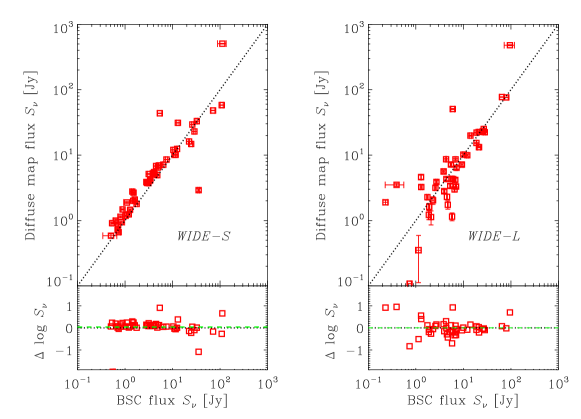
Figure 1: Comparison between the AKARI FISBSC flux density and that measured from the diffuse map at WIDE-S (left) and WIDE-L (right). Diagonal lines represent $y=x$. The lower panels show the logarithmic deviation of data from the diagonal lines. Horizontal dashed lines are the average deviation of data at each band.

The AKARI FISBSC was produced by a dedicated pipeline for point source extraction (Yamamura et al., 2010). However, for very extended nearby galaxies, the point source assumption is not valid anymore. To examine this “aperture” effect in AKARI FIS flux density, we measured IR flux density from AKARI FIS diffuse map. We performed this procedure by using both SExtractor (Bertin & Arnouts, 1996) and our own software, and both yielded more or less the same result. Since Yuan et al. (2011) used SExtractor, we also present flux density given by SExtractor for the diffuse map. We show the comparison between flux densities from FISBSC and diffuse map for M99 sample in Fig. 1.

Basically these flux densities agree well, because M99 put a constraint to have galaxies with a small angular diameter in their sample selection. However, even so, the BSC flux density turned out to be underestimated for non-negligible number of galaxies. The horizontal dashed lines represent the average difference between BSC and diffuse-map flux densities. For both WIDE-S and WIDE-L, the average is positive. Yuan et al. (2011) performed a careful comparison of BSC flux density with other well-understood database and concluded that this is due to the underestimation of the BSC and not the overestimation in diffuse map photometry. Thus, we use the diffuse-map based IR flux densities to have the final IRX-$\beta$ relation fitting.

References

- Bertin & Arnouts (1996) Bertin, E., & Arnouts, S. 1996, A&AS, 117, 393
- Bouwens et al. (2004) Bouwens, R. J., et al. 2004, ApJ, 606, L25
- Bouwens et al. (2007) Bouwens, R. J., Illingworth, G. D., Franx, M., & Ford, H. 2007, ApJ, 670, 928
- Bouwens et al. (2009) Bouwens, R. J., et al. 2009, ApJ, 705, 936
- Bell et al. (2005) Bell, E. F., et al. 2005, ApJ, 625, 23
- Boissier et al. (2007) Boissier, S., et al. 2007, ApJS, 173, 524
- Bouquien et al. (2009) Bouquien, M., et al. 2009, ApJ, 706, 533
- Buat et al. (2002) Buat, V., Boselli, A., Gavazzi, G., & Bonfanti, C. 2002, A&A, 383, 801
- Buat et al. (2005) Buat, V., Iglesias-Páramo, J, Seibert, M. et al. 2005, ApJ, 619, L51
- Buat et al. (2007a) Buat, V., Takeuchi, T. T., Iglesias-Páramo, J, et al. 2007a, ApJS, 173, 404
- Buat et al. (2007b) Buat, V., Marcillac, D., Burgarella, D. et al. 2007b, A&A, 469, 19
- Buat et al. (2010) Buat, V., et al. 2010, MNRAS, 409, 1
- Burgarella et al. (2005a) Burgarella, D., Buat, V., & Iglesias-Páramo, J. 2005, MNRAS, 360, 1413
- Burgarella et al. (2005b) Burgarella, D., et al. 2005, ApJ, 619, L63
- Calzetti et al. (1994) Calzetti, D., Kinney, A. L., & Storchi-Bergmann, T. 1994, ApJ, 429, 582
- Calzetti et al. (2000) Calzetti, D., Armus, L., Bohlin, R. C., Kinney, A. L., Koornneef, J., & Storchi-Bergmann, T. 2000, ApJ, 533, 682
- Cardelli et al. (1989) Cardelli, J. A., Clayton, G. C., & Mathis, J. S. 1989, ApJ, 345, 245
- Connolly et al. (1997) Connolly, A. J., Szalay, A. S., Dickinson, M., Subbarao, M. U., & Brunner, R. J. 1997, ApJ, 486, L11
- Conroy et al. (2010) Conroy, C., Schiminovich, D., & Blanton, M. R. 2010, ApJ, 718, 184
- Cortese et al. (2006) Cortese, L., et al. 2006, ApJ, 637, 242
- Dale et al. (2001) Dale, D. A., et al. 2001, ApJ, 549, 215
- Dale & Helou (2002) Dale, D. A. , Helou, G. 2002, ApJ, 576, 159
- Dale et al. (2005) Dale, D. A. , et al. 2005, ApJ, 633, 857
- Daddi et al. (2007) Daddi, E., et al. 2007, ApJ, 670, 156
- Draine (2003) Draine, B. T. 2003, ARA&A, 41, 241
- Draine (2009) Draine, B. T. 2009, in Cosmic Dust – Near and Far, Astronomical Society of the Pacific Conference Series, 414, 453
- Dwek & Scalo (1980) Dwek, E., & Scalo, J. M. 1980, ApJ, 239, 193
- Dwek (1998) Dwek, E. 1998, ApJ, 501, 643
- Gil de Paz et al. (2007) Gil de Paz, A., et al. 2007, ApJS, 173, 185
- Goldader et al. (2002) Goldader, J. D., Meurer, G., Heckman, T. M., Seibert, M., Sanders, D. B., Calzetti, D., & Steidel, C. C. 2002, ApJ, 568, 651
- Helou et al. (1988) Helou, G., Khan, I. R., Malek, L., & Boehmer, L. 1988, ApJS, 68, 151
- Hirashita et al. (2003) Hirashita, H., Buat, V., & Inoue, A. K. 2003, A&A, 410, 83
- Hirashita et al. (2008) Hirashita, H., Kaneda, H., Onaka, T., & Suzuki, T. 2008, PASJ, 60, 477
- Iglesias-Páramo et al. (2006) Iglesias-Páramo, J., Buat, V., Takeuchi, T. T., et al. 2006, ApJS, 164, 38
- Inoue (2002) Inoue, A. K. 2002, ApJ, 570, L97
- Kawada et al. (2007) Kawada, M., et al. 2007, PASJ, 59, 389
- Kawada et al. (2008) Kawada, M., et al. 2008, PASJ, 60, 389
- Kennicutt et al. (1994) Kennicutt, R. C., Jr., Tamblyn, P., & Congdon, C. E. 1994, ApJ, 435, 22
- Kennicutt et al. (2003) Kennicutt, R. C., Jr., et al. 2003, PASP, 115, 928
- Kinney et al. (1993) Kinney, A. L., Bohlin, R. C., Calzetti, D., Panagia, N., & Wyse, R. F. G. 1993, ApJS, 86, 5
- Kong et al. (2004) Kong, X., Charlot, S., Brinchmann, J., & Fall, S. M. 2004, MNRAS, 349, 769
- Leitherer & Heckman (1995) Leitherer, C., & Heckman, T. M. 1995, ApJS, 96, 9
- Lilly et al. (1996) Lilly, S. J., Le Févre, O., Hammer, F., & Crampton, D. 1996, ApJ, 460, L1
- Madau et al. (1996) Madau, P., Ferguson, H. C., Dickinson, M. E., Giavalisco, M., Steidel, C. C., & Fruchter, A. 1996, MNRAS, 283, 1388
- Madau et al. (1998) Madau, P., Pozzetti, L., & Dickinson, M. 1998, ApJ, 498, 106
- Meurer et al. (1999) Meurer, G. R., Heckman, T. M., & Calzetti, D. 1999, ApJ, 521, 64
- Meurer et al. (1995) Meurer, G. R., Heckman, T. M., Leitherer, C., Kinney, A., Robert, C., & Garnett, D. R. 1995, AJ, 110, 2665
- Morrissey et al. (2007) Morrissey, P., et al. 2007, ApJS, 173, 682
- Muñoz-Mateos et al. (2009) Muñoz-Mateos, J. C., et al. 2009, ApJ, 701, 1965
- Nozawa et al. (2003) Nozawa, T., Kozasa, T., Umeda, H., Maeda, K., & Nomoto, K. 2003, ApJ, 598, 785
- Nozawa et al. (2010) Nozawa, T., Kozasa, T., Tominaga, N., Maeda, K., Umeda, H., Nomoto, K., & Krause, O. 2007, ApJ, 666, 955
- Onaka et al. (2007) Onaka, T., et al. 2007, PASJ, 59, S401
- Overzier et al. (2011) Overzier, R. A., et al. 2011, ApJ, 726, L7
- Petrosian et al. (1972) Petrosian, V., Silk, J., & Field, G. B. 1972, ApJ, 177, L69
- Pettini et al. (1998) Pettini, M., Kellogg, M., Steidel, C. C., Dickinson, M., Adelberger, K. L., & Giavalisco, M. 1998, ApJ, 508, 539
- Reddy et al. (2010) Reddy, N. A., Erb, D. K., Pettini, M., Steidel, C. C., & Shapley, A. E. 2010, ApJ, 712, 1070
- Rigopoulou et al. (1996) Rigopoulou, D., Lawrence, A., & Rowan-Robinson, M. 1996, MNRAS, 278, 1049
- Sakurai et al. (2011) Sakurai, A., Takeuchi, T. T., Yuan, F.-T., Buat, V., & Burgarella, D., 2011, Earth, Planets and Space, submitted
- Salpeter (1955) Salpeter, E. E. 1955, ApJ, 121, 161
- Sanders & Mirabel (1996) Sanders, D. B., & Mirabel, I. F. 1996, ARA&A, 34, 749
- Saunders et al. (2000) Saunders, W., et al. 2000, MNRAS, 317, 55
- Schlegel et al. (1998) Schlegel, D. J., Finkbeiner, D. P., & Davis, M. 1998, ApJ, 500, 525
- Seibert et al. (2005) Seibert, M., et al. 2005, ApJ, 619, L55
- Siana et al. (2008) Siana, B., Teplitz, H. I., Chary, R.-R., Colbert, J., & Frayer, D. T. 2008, ApJ, 689, 59
- Siana et al. (2009) Siana, B., et al. 2009, ApJ, 698, 1273
- Smith et al. (1978) Smith, L. F., Biermann, P., & Mezger, P. G. 1978, A&A, 66, 65
- Spergel et al. (2007) Spergel, D. N., et al. 2007, ApJS, 170, 377
- Takeuchi et al. (2003) Takeuchi, T. T., Hirashita, H., Ishii, T. T., Hunt, L. K., & Ferrara, A. 2003, MNRAS, 343, 839
- Takeuchi et al. (2005a) Takeuchi, T. T., Buat, V., Burgarella, D. 2005a, A&A, 440, L17
- Takeuchi et al. (2005b) Takeuchi, T. T., Buat, V.,Iglesias-Páramo, J, Boselli, A., Burgarella, D. 2005b, A&A, 432, 423
- Takeuchi et al. (2005c) Takeuchi, T. T., Ishii, T. T., Nozawa, T., Kozasa, T., & Hirashita, H. 2005c, MNRAS, 362, 592
- Takeuchi et al. (2010) Takeuchi, T. T., Buat, V., Heinis, S., Giovannoli, E., Yuan, F.-T., Iglesias-Páramo, J., Murata, K. L., & Burgarella, D. 2010, A&A, 514, A4
- Tinsley & Danly (1980) Tinsley, B. M., & Danly, L. 1980, ApJ, 242, 435
- Yamamura et al. (2010) Yamamura, I., Makiuti, S., Ikeda, N., Fukuda, Y., Oyabu, S., Koga, T., White, G. J. 2010, AKARI/FIS All-Sky Survey Bright Source Catalogue Version 1.0 Release Note
- Yuan et al. (2011) Yuan, F.-T., Takeuchi, T. T., Buat, V., Heinis, S., Giovannoli, E., Murata, K. L., Iglesias-Páramo, & Burgarella, D. 2011, PASJ, 63, 1207