On the half-space theorem
for minimal surfaces in Heisenberg space

Abstract.

We propose a simple proof of the vertical half-space theorem for Heisenberg space.

1. Introduction

A half-space theorem states that the only properly immersed minimal surface which is contained in a half-space is a parallel translate of the boundary of the half-space, namely a plane. Hoffman and Meeks first proved it for $\mathbb{R}^{3}$ ([HM]). It fails in $\mathbb{R}^{n}$ or $\mathbb{H}^{n}$, $n\geq 4$.

In recent years, there has been increased interest in homogeneous $3$-manifolds (cf. Abresh/Rosenberg [AR1], Hauswirth/Rosenberg/Spruck [HRS]). The original proof of Hoffman and Meeks also works in Heisenberg space $\operatorname{Nil}_{3}$ with respect to umbrellas, which are the exponential image of a horizontal tangent plane ([AR2]). Daniel and Hauswirth extended the theorem to vertical half-spaces of Heisenberg space, where vertical planes are defined as the inverse image of a straight line in the base of the Riemannian fibration $\operatorname{Nil}_{3}\to\mathbb{R}^{2}$ ([DH]).

Vertical half-space theorem in Heisenberg space (Daniel/Hauswirth 2009).

Let $S$ be a properly immersed minimal surface in Heisenberg space. If $S$ lies to one side of a vertical plane $P$, then $S$ is a plane parallel to $P$.

Essential for the proof of half-space theorems is the existence of a family of catenoids or generalized catenoids. Their existence is simple to establish in spaces where they can be represented as ODE solutions. For instance, horizontal umbrellas in Heisenberg space are invariant under rotations around the vertical axis, so they lead to an ODE. However, the lack of rotations about horizontal axes means that the existence of analogues of a horizontal catenoid amounts to establishing true PDE solutions. Daniel and Hauswirth use a Weierstraß-type representation to reduce this problem to a system of ODEs. Only after solving a period problem they obtain the desired family of surfaces.

In the present paper we introduce a simpler approach: we take a coordinate model of Heisenberg space and consider coordinate surfaces of revolution. Provided we can choose a family of surfaces whose mean curvature normal points into the half-space, the original maximum principle argument of Hoffman and Meeks will prove the theorem. Our approach is based on an idea by Bergner ([B]), who generalized the classical half-space theorem to surfaces with negative Gaussian curvature such that the principal curvatures satisfy an inequality, and Earp / Toubiana ([ET]), who consider special Weingarten surfaces with mean curvature satisfying an inequality.

It is an open problem to prove a vertical half-space theorem for $\operatorname{PSL}_{2}(\mathbb{R})$, where it would apply to surfaces whose mean curvature is the so-called magic number $H_{0}=1/2$, namely the limiting value of the mean curvature of large spheres. Here, it would state that surfaces with mean curvature $H_{0}=1/2$ lying on the mean convex side of a horocylinder can only be horocylinders, that is, the inverse image of a horocycle of the fibration $\operatorname{PSL}_{2}(\mathbb{R})\to\mathbb{H}^{2}$. Our strategy could also work there. However, so far we have not been successful to establish the desired family of generalized catenoids with $H\leq H_{0}$.

I would like to thank my advisor Karsten Große-Brauckmann for his help.

2. The Euclidean half-space theorem

Euclidean half-space theorem (Hoffman/Meeks 1990).

A properly immersed minimal surface $S$ in $\mathbb{R}^{3}$ lying in a half-space $H$ is a plane parallel to $P=\partial H$.

Proof.

By the standard maximum principle we can assume $\operatorname{dist}(S,P)=0$ but $S\cap P=\emptyset$.

Let $\mathcal{C}_{r}\subset\mathbb{R}^{3}\setminus H$ be a half catenoid with necksize $r$ and $\partial\mathcal{C}_{r}\subset P$. By the properness of $S$, we can translate $S$ by $\varepsilon>0$ towards $\mathcal{C}_{1}$ such that $S$ intersects $P$ but stays disjoint to $\partial\mathcal{C}_{r}$ for all $r\in(0,1]$.

As $r$ tends to $0$, the family of catenoids $\mathcal{C}_{r}$ converges to $P$ minus a point. We claim that the set $I$ of parameters for which $\mathcal{C}_{r}$ does not intersect $S$ is open. Consider a catenoid $\mathcal{C}_{r_{0}}$ that does not intersect $S$. For each $r\in(0,1)$ there exists a compact set $K$ such that the distance between $\mathcal{C}_{r}$ and $P$ is larger than $2\varepsilon$ in the complement of $K$. We may choose $K$ in a way that this property holds for all $r$ in a small neighbourhood of $r_{0}$. This implies that the distance between $S$ and all these $\mathcal{C}_{r}$ is larger than $\varepsilon$ in the complement of $K$ (cf. figure 1).

However, within the compact set $K$, the distance between $S$ and $C_{r_{0}}$ is positive, so for all $r$ in a (possibly smaller) neighbourhood of $r_{0}$, this distance is still positive.

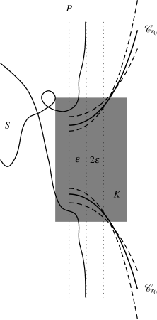
Figure 1. Proof of the Euclidean half-space theorem

We conclude that in small neighbourhood of $r_{0}$,

$$\operatorname{dist}(\mathcal{C}_{r},S)\geq\min(\operatorname{dist}(\mathcal{C}_{r}\cap K,S\cap K),\operatorname{dist}(\mathcal{C}_{r}\cap K^{c},S\cap K^{c}))>0,$$

thereby proving our claim.

Therefore, the set of parameters for which $\mathcal{C}_{r}$ and $S$ do intersect is closed, so there is a first catenoid $\mathcal{C}_{r_{1}}$ touching $S$ at a point $p$. Since the boundaries of all $\mathcal{C}_{r}$ with $r\in(0,1]$ are disjoint from $S$, the touching point $p$ is an interior point, contradicting the maximum principle. ∎

3. Coordinate surfaces of revolution

We take the following coordinates:

$$\operatorname{Nil}_{3} :=(\mathbb{R}^{3},\mathrm{d}s^{2}), \mathrm{d}s^{2} =\mathrm{d}x^{2}+\mathrm{d}y^{2}+(2\tau x\mathrm{d}y-\mathrm{d}z)^{2} \text{with }\tau \geq 0.$$

An orthonormal frame of the tangent space is given by

$$E_{1} =\partial_{x}, E_{2} =\partial_{y}+2\tau x\partial_{z}, E_{3} =\partial_{z},$$

and the Riemannian connection in these coordinates is determined by

(1) $$\nabla_{E_{1}}E_{2} =-\nabla_{E_{2}}E_{1}=\tau E_{3}, \nabla_{E_{1}}E_{3} =\nabla_{E_{3}}E_{1}=-\tau E_{2},$$

$$\nabla_{E_{2}}E_{3} =\nabla_{E_{3}}E_{2}=\tau E_{1}, \nabla_{E_{i}}E_{j} =0\text{ in all other cases.}$$

The Heisenberg space is a Riemannian fibration $\pi\colon\mathbb{R}^{3}\to\mathbb{R}^{2}$ with vanishing base curvature. The bundle curvature of $\operatorname{Nil}_{3}$ is given by $\frac{1}{2}g(\nabla_{E_{1}}E_{2}-\nabla_{E_{2}}E_{1},E_{3})=\tau$ and for $\tau=0$ we recover $\mathbb{R}^{3}$.

Let us consider a curve $c(t)=(0,t,r(t))$ in Heisenberg space with a positive function $r$ and $t\geq 0$. By rotating around the $y$-axis, we get an immersion

$$f\colon[t_{0},\infty)\times[0,2\pi)\to\operatorname{Nil}_{3},\quad(t,\varphi)\mapsto\begin{pmatrix}-r(t)\sin\varphi\\ t\\ r(t)\cos\varphi\end{pmatrix}.$$

In order to apply the proof of Hoffman/Meeks, we will construct Euclidean rotational surfaces around the $y$-axis. With the Heisenberg space metric, these rotations are not isometric, because the $4$-dimensional isometry group of $\operatorname{Nil}_{3}$ contains only translations and rotations around the vertical axis. Therefore, the mean curvature of such a surface will depend on the angle of rotation $\varphi$. We will need to find a surface with mean curvature vector pointing to the half-space to arrive at the desired contradiction with the maximum principle.

The tangent space of $M:=f([t_{0},\infty)\times[0,2\pi))$ is spanned by

$$v_{1} =-r^{\prime}(t)\sin\varphi E_{1}+E_{2}+(2\tau r(t)\sin\varphi+r^{\prime}(t)\cos\varphi)E_{3},$$

$$v_{2} =-r(t)\cos\varphi E_{1}-r(t)\sin\varphi E_{3},$$

so the inner normal of $M$ is

$$N=\frac{1}{W}(\sin\varphi E_{1}+(r^{\prime}(t)+2\tau r(t)\sin\varphi\cos\varphi)E_{2}-\cos\varphi E_{3}),$$

where $W=\sqrt{1+(2\tau r(t)\sin\varphi\cos\varphi+r^{\prime}(t))^{2}}$.

We will now compute the first and second fundamental forms of $M$. We easily get

$$G_{ij} =\mathrm{d}s^{2}(v_{i},v_{j})$$

$$=\begin{pmatrix}\sin^{2}\!\varphi\,r^{\prime}(t)^{2}+\left(2\tau r(t)\sin\varphi+\cos\varphi r^{\prime}(t)\right)^{2}+1&-2\tau r(t)^{2}\sin^{2}\varphi\\ -2\tau r(t)^{2}\sin^{2}\varphi&r(t)^{2}\\ \end{pmatrix}$$

with determinant $\det G=r(t)^{2}W^{2}$.

The most tedious part of the calculation is the second fundamental form. We have to compute $B_{ij}=\mathrm{d}s^{2}(\nabla_{v_{i}}v_{j},N)$. To start, (1) gives

$$\nabla_{v_{1}}E_{1} =(-2\tau^{2}r(t)\sin\varphi-\tau r^{\prime}(t)\cos\varphi)E_{2}-\tau E_{3},$$

$$\nabla_{v_{1}}E_{2} =(2\tau^{2}r(t)\sin\varphi+\tau r^{\prime}(t)\cos\varphi)E_{1}-\tau r^{\prime}(t)\sin\varphi E_{3},$$

$$\nabla_{v_{1}}E_{3} =\tau E_{1}+\tau r^{\prime}(t)\sin\varphi E_{2}.$$

We calculate

$$\nabla_{v_{1}}v_{1}= -r^{\prime\prime}(t)\sin\varphi E_{1}+(2\tau r^{\prime}(t)\sin\varphi+r^{\prime\prime}(t)\cos\varphi)E_{3}$$

$$-r^{\prime}(t)\sin\varphi\nabla_{v_{1}}E_{1}+\nabla_{v_{1}}E_{2}+(2\tau r(t)\sin\varphi+r^{\prime}(t)\cos\varphi)\nabla_{v_{1}}E_{3}$$

$$= (-r^{\prime\prime}(t)\sin\varphi+4\tau^{2}r(t)\sin\varphi+2\tau r^{\prime}(t)\cos\varphi)E_{1}$$

$$+(4\tau^{2}r(t)r^{\prime}(t)\sin^{2}\varphi+2\tau r^{\prime}(t)^{2}\sin\varphi\cos\varphi)E_{2}$$

$$+(2\tau r^{\prime}(t)\sin\varphi+r^{\prime\prime}(t)\cos\varphi)E_{3},$$

and obtain the first entry of $B$ as

$$B_{11}=\frac{1}{W}\bigg{(}-r^{\prime\prime}(t)+4\tau^{2}r(t)r^{\prime}(t)^{2}\sin^{2}(\varphi)+8\tau^{3}r(t)^{2}r^{\prime}(t)\sin^{3}(\varphi)\cos(\varphi)+4\tau^{2}r(t)\sin^{2}(\varphi)$$

$$+2\tau r^{\prime}(t)^{3}\sin(\varphi)\cos(\varphi)+4\tau^{2}rr^{\prime 2}\sin^{2}(\varphi)\cos^{2}(\varphi)\bigg{)}.$$

The other three entries arise similarly from

$$\nabla_{v_{2}}v_{1}=\nabla_{v_{1}}v_{2}= -(\tau r(t)\sin\varphi+r^{\prime}(t)\cos\varphi)E_{1}$$

$$+(\tau r(t)\left(2\tau r(t)\sin\varphi\cos\varphi+r^{\prime}(t)\cos(2\varphi\right))E_{2}$$

$$+(\tau r(t)\cos\varphi-r^{\prime}(t)\sin\varphi)E_{3},$$

$$\nabla_{v_{2}}v_{2}= r(t)\sin\varphi E_{1}-2\tau r(t)^{2}\sin\varphi\cos\varphi E_{2}-r(t)\cos\varphi E_{3}.$$

They are

$$B_{12}=B_{21} =\frac{\tau r(t)\left(4\tau r(t)r^{\prime}(t)\sin\varphi\cos^{3}\varphi+\tau^{2}r(t)^{2}\sin^{2}(2\varphi)+\cos(2\varphi)r^{\prime}(t)^{2}-1\right)}{W},$$

$$B_{22} =-\frac{r(t)\left(\tau r(t)\sin(2\varphi)\left(\tau r(t)\sin(2\varphi)+r^{\prime}(t)\right)-1\right)}{W}.$$

We obtain the mean curvature $H$ for our coordinate surface of revolution:

Lemma 1.

The mean curvature $H=H(t,\varphi)$ of $f$ is given by

$$H :=\frac{1}{2}\operatorname{tr}(G^{-1}B)$$

$$=\frac{G_{22}B_{11}-G_{12}B_{21}-G_{21}B_{12}+G_{11}B_{22}}{2r(t)^{2}W^{2}}$$

$$=\frac{1+r^{\prime}(t)^{2}-r(t)r^{\prime\prime}(t)+4\tau^{2}r(t)^{2}\sin^{4}\varphi+2\tau r(t)r^{\prime}(t)\sin\varphi\cos\varphi}{2r(t)W^{3}}.$$

4. Half-space theorem in Heisenberg space

As expected, for $\tau=0$ Lemma 1 recovers the mean curvature for rotational surfaces in Euclidean space. For $\tau\neq 0$, the two additional terms depending on $\varphi$ in the nominator of $H$ arise because the horizontal rotation is not an isometry of Heisenberg space. Our goal is to exhibit a family of rotational surfaces satisfying $H\leq 0$ with respect to the normal $N$.

Consider the rotational surface $f_{c}$ given in terms of

(2) $$r_{c}(t):=\exp\left(\frac{1}{c}\exp(ct)\right)$$

with $c>c_{0}:=4\tau^{2}+2\tau+1$. We claim that this surface satisfies $H\leq 0$ for $t>0$. Indeed, the following estimate for the denominator of $H$ holds:

$$2r(t)W^{3}H \leq 1+r_{c}^{\prime}(t)^{2}-r_{c}(t)r_{c}^{\prime\prime}(t)+4\tau^{2}r_{c}(t)^{2}+2\tau r_{c}(t)r_{c}^{\prime}(t)$$

$$=1+r_{c}(t)^{2}(\exp(ct)(2\tau-c)+4\tau^{2})$$

$$\leq 1+r_{c}(t)^{2}(4\tau^{2}+2\tau-c)\leq 1+4\tau^{2}+2\tau-c\leq 0.$$

Since we consider a rotational surface with an embedded meridian, the embeddedness of $M_{c}:=f_{c}([t_{0},\infty)\times[0,2\pi))$ is obvious. Also, the boundary $\partial M_{c}=\{\exp(1/c)\cdot(\sin\varphi,0,\cos\varphi)\colon\varphi\in[0,2\pi)\}$ is explicitly known.

It is also important to note that for each $c$ and any given $\varepsilon>0$, there exists a compact set such that the distance between $M_{c}$ and the plane $\{y=0\}$ is larger than $\varepsilon$ in the complement of this compact set.

Let us summarize the result:

Lemma 2.

The coordinate surface of revolution whose meridian is defined by (2) satisfies for $c>c_{0}$

1. $H\leq 0$ with respect to the normal $N$,

2. for $c\to\infty$, the surface $M_{c}$ converges uniformly to a subset of $\{y=0\}$ on compact sets,

3. $M_{c}$ is properly embedded,

4. $\partial M_{c}=\{\exp(1/c)\cdot(\sin\varphi,0,\cos\varphi)\colon\varphi\in[0,2\pi)\}$ for all $c$.

Using the surfaces $M_{c}$, our proof of the Euclidean half-space theorem literally applies to Heisenberg space.