Sampled-data design for robust control of a single qubit

Abstract

This paper presents a sampled-data approach for the robust control of a single qubit (quantum bit). The required robustness is defined using a sliding mode domain and the control law is designed offline and then utilized online with a single qubit having bounded uncertainties. Two classes of uncertainties are considered involving the system Hamiltonian and the coupling strength of the system-environment interaction. Four cases are analyzed in detail including without decoherence, with amplitude damping decoherence, phase damping decoherence and depolarizing decoherence. Sampling periods are specifically designed for these cases to guarantee the required robustness. Two sufficient conditions are presented for guiding the design of unitary control for the cases without decoherence and with amplitude damping decoherence. The proposed approach has potential applications in quantum error-correction and in constructing robust quantum gates.

Nomenclature

Throughout this paper, we use the following notation:
$|\psi\rangle$         state vector (quantum pure state)
$a^{*}$          complex conjugate of $a$
$L^{T}$          transpose of $L$
$L^{\dagger}$          adjoint of $L$
$\text{tr}(A)$       trace of $A$
$\langle\psi|$         adjoint of $|\psi\rangle$
$\langle\phi|\psi\rangle$      inner product of $|\phi\rangle$ and $|\psi\rangle$
$\rho$           density operator
$\sigma_{x,y,z}$       Pauli matrices
$\omega(t)$         uncertainty amplitude in $\sigma_{z}$
$\epsilon_{x}(t)$       uncertainty amplitude in $\sigma_{x}$
$\epsilon_{y}(t)$        uncertainty amplitude in $\sigma_{y}$
$\mathbf{R}$         set of real numbers
$\gamma$          coupling strength
$\delta\gamma_{t}$       uncertainty in coupling strength
$\mathcal{D}_{c}$        sliding mode domain of closed systems
$\mathcal{D}_{a}$        sliding mode domain of quantum systems with amplitude damping decoherence
$\mathcal{D}_{p}$        sliding mode domain of quantum systems with phase damping decoherence
$\mathcal{D}_{d}$        sliding mode domain of quantum systems with depolarizing decoherence
$C$         coherence
$P$          purity
$p_{0}$        probability of failure

I INTRODUCTION

Controlling quantum phenomena is becoming an important task in different research areas such as quantum optics, physical chemistry and quantum information [1]-[4]. The development of quantum control theory can provide systematic methods and a theoretical framework for analyzing and synthesizing quantum control problems. Several theoretical tools and design methods in classical control have been applied to the quantum domain. For example, Lie groups and Lie algebras have been used to establish controllability conditions for closed quantum systems [5]. Optimal control theory has been applied to control analysis and the design of several quantum control tasks such as population transfer with minimum energy or in the shortest time [6]-[9]. Learning control has become a powerful tool for the direct laboratory discovery of laser pulses controlling a variety of atomic and molecular phenomena [3]. Feedback control has been utilized for the control of quantum entanglement, quantum error-correction and quantum state preparation [10]-[20]. The development of quantum control theory needs to consider the special characteristics of quantum systems (e.g., measurement collapse and non-commutative relationships) and the unique objectives of quantum control (e.g., entanglement generation and decoherence control) (For more discussion, see, e.g., [1]).

Robust control is one of the most important research areas in classical control theory. Attaining robust control for quantum systems has been recognized as a key issue in the development of practical quantum technology [21]-[25], since many types of uncertainties are unavoidable (including control noise, environmental disturbances, etc.) for most practical quantum systems. Several methods have been proposed for the robust control of quantum systems. For example, James et al. [26] formulated and solved a quantum robust control problem using the $H^{\infty}$ method for linear quantum stochastic systems. A risk-sensitive control problem has been solved for a sampled-data feedback model of quantum systems [27]. Quantum robust control is still in its infancy, and it is necessary to develop new tools to deal with different types of uncertainties.

Dong and Petersen [28]-[30] developed sliding mode control to enhance the robustness of quantum systems. In particular, two approaches based on sliding mode design [31] have been proposed for the control of quantum systems, and potential applications of sliding mode control to quantum information processing have been presented [28]. Sliding mode control for two-level quantum systems was presented to deal with bounded uncertainties in the system Hamiltonian [29]. This paper will employ the concept of a sliding mode domain to define the required robustness and develop a new sampled-data design approach [32], [33] to enhance the performance of a controlled quantum system with uncertainties in the Hamiltonian as well as in the system-environment interaction.

Sampled-data control has been widely applied in industrial electronics, process control and signal processing [33]. The sampled data are used to design controllers while the sampling (measurement) process is usually assumed not to affect the system’s state. However, in quantum control, the sampling process unavoidably destroys the system’s state according to the measurement collapse postulate (see, e.g., [4]). Hence, measurement can be used as the means for information acquisition as well as a control tool. For example, several incoherent control schemes have been presented where measurements are used as a control tool to affect the system dynamics [34]-[36]. A framework of quantum operations including unitary control and projective measurements has been developed to investigate feedback control of quantum systems [37], [38]. One well known example where measurement modifies the system dynamics is the quantum Zeno effect, which is the inhibition of transitions between quantum states by frequent measurement of the state (see, e.g., [39] and [40]). However, it is usually a difficult task to make frequent measurements with practical quantum systems. We may assume that the smaller the measurement period is, then the bigger the cost of accomplishing the periodic measurements becomes. Hence, in contrast to the quantum Zeno effect, in this paper we will use the sampling (projective measurement) process as a control tool and design sampling periods as large as possible to guarantee the required robustness for several classes of quantum control tasks including control design for quantum systems with uncertainties in the system Hamiltonian and robust decoherence control of Markovian open quantum systems.

Decoherence occurs when a quantum system interacts with an uncontrollable environment [41]. Decoherence has been recognized as a bottleneck for the development of practical quantum information technology [42]. Various methods have been proposed for decoherence control including quantum error-avoiding codes [43]-[45], quantum error-correction codes [46], dynamical decoupling [47], [48] and quantum feedback control [49]. In quantum error-avoiding codes, quantum information is encoded in a decoherence free subspace which is inherently immune to decoherence due to specific symmetries in the system-environment interaction [50]. Quantum error-correction codes are active methods to detect and counteract the effects of errors during quantum information processing via encoding redundant qubits. Dynamical decoupling of decoherence control is an open-loop control approach which often employs bang-bang control pulses to dynamically cancel the effect of decoherence. Quantum feedback and optimal control theory also provide powerful tools for the analysis and design of decoherence control [51], [52]. However, there are few results which consider robustness when uncertainties or inaccurate parameters exist in the system Hamiltonian or the system-environment interaction. Here we consider a robust decoherence control scheme for quantum systems subject to Markovian decoherence [4]. In particular, we will focus on a single qubit subject to amplitude damping decoherence, phase damping decoherence and depolarizing decoherence [4]. We propose a sampling-based design approach to guarantee the robustness of a single qubit system with uncertainties in the system Hamiltonian and the coupling strength of the system-environment interaction.

The paper is organized as follows. Section II presents the control problem formulation and defines the required robustness. In Section III, we present the main methods and results for robust control design. Section IV gives the proofs of the main results. Concluding remarks are given in Section V.

II Control problem formulation

For an open quantum system, its state is described by the positive Hermitian density matrix (or density operator) $\rho$ satisfying $\text{tr}\rho=1$, and the evolution of $\rho$ cannot generally be described in terms of a unitary transformation. In many situations, a quantum master equation for $\rho(t)$ (or $\rho_{t}$) is a suitable way to describe the dynamics of an open quantum system. One of the simplest cases is when a Markovian approximation can be applied under the assumption of a short environmental correlation time permitting the neglect of memory effects [41]. For an $N$-dimensional open quantum system with Markovian dynamics, its state $\rho(t)$ can be described by the following Markovian master equation (for details, see, e.g., [41], [53], [54]):

$$\dot{\rho}(t)=-i[H(t),\rho(t)]+\frac{1}{2}\sum_{j,k=0}^{N^{2}-1}\alpha_{jk}\{[L_{j}\rho(t),L^{\dagger}_{k}]+[L_{j},\rho(t)L^{\dagger}_{k}]\}.$$ (1)

Here for an arbitrary operator $X$, $[X,\rho]=X\rho-\rho X$ is the commutation operator, $\{L_{j}\}_{j=0}^{N^{2}-1}$ is a basis for the space of linear bounded operators on the Hilbert space $\mathcal{H}$ with $L_{0}=I$, the coefficient matrix $A=(\alpha_{jk})$ is positive semidefinite and physically specifies the relevant relaxation rates and we have set $\hbar=1$ in this paper. Markovian master equations have been widely used to model controlled quantum systems in quantum control [55]-[57], especially for Markovian quantum feedback [2].

In this paper, we will focus on a two-level quantum system (a single qubit) with Markovian dynamics whose evolution can be described by the following Lindblad equation:

$$\dot{\rho}(t)=-i[H(t),\rho(t)]+\sum_{k=1}^{K}\gamma_{k}\mathfrak{D}[L_{k}]\rho(t),$$ (2)

where

$$\mathfrak{D}[L_{k}]\rho=L_{k}\rho L_{k}^{{\dagger}}-\frac{1}{2}L_{k}^{{\dagger}}L_{k}\rho-\frac{1}{2}\rho L_{k}^{{\dagger}}L_{k}.$$

For such a single qubit system, we can divide $H(t)$ into three parts $H(t)=H_{0}+H_{\Delta}+H_{u}$, where the free Hamiltonian is $H_{0}=\frac{1}{2}\sigma_{z}$, the control Hamiltonian is $H_{u}=\sum_{j=x,y,z}u_{j}(t)I_{j}$, ($u_{j}(t)\in\mathbf{R}$, $I_{j}=\frac{1}{2}\sigma_{j}$), and the uncertainties in the system Hamiltonian are $H_{\Delta}=\omega(t)I_{z}+\epsilon_{x}(t)I_{x}+\epsilon_{y}(t)I_{y}$ ($\omega(t),\epsilon_{x}(t),\epsilon_{y}(t)\in\mathbf{R}$). The Pauli matrices $\sigma=(\sigma_{x},\sigma_{y},\sigma_{z})$ take the following form:

$$\sigma_{x}=\begin{pmatrix}0&1\\ 1&0\\ \end{pmatrix},\ \ \ \ \sigma_{y}=\begin{pmatrix}0&-i\\ i&0\\ \end{pmatrix},\ \ \ \ \sigma_{z}=\begin{pmatrix}1&0\\ 0&-1\\ \end{pmatrix}.$$ (3)

$H_{\Delta}$ is the first class of uncertainties we will consider in this paper. The unitary errors in [21] belong to this class of uncertainties, and one-qubit gate errors also correspond to this class of uncertainties [28]. A second class of uncertainties are uncertainties $\delta\gamma_{k}$ residing in the coupling strength $\gamma_{k}$. Since the Lindblad equation is an approximate equation for the open quantum system coupling with its environment, this class of uncertainties may come from inaccurate modeling as well as time-varying coupling between the system and environment. We assume that all the uncertainties are bounded, i.e., $|\omega(t)|\leq\omega$, $\sqrt{\epsilon_{x}^{2}(t)+\epsilon_{y}^{2}}\leq\epsilon$ and $|\delta\gamma_{k}|\leq\gamma$, where constants $\omega\geq 0$, $\epsilon>0$ and $\gamma\geq 0$ are given.

For a qubit system, its state $\rho$ can be represented in terms of the Bloch vector $\mathbf{r}=(x,y,z)=(\text{tr}\{\rho\sigma_{x}\},\text{tr}\{\rho\sigma_{y}\},\text{tr}\{\rho\sigma_{z}\})$:

$$\rho=\frac{I+\mathbf{r}\cdot\sigma}{2}.$$ (4)

After representing the state $\rho$ with the Bloch vector, the pure states (i.e., with $\text{tr}(\rho^{2})=1$) for the qubit system lie on the surface of the Bloch sphere and the mixed states (i.e., with $\text{tr}(\rho^{2})<1$) occupy the interior of the Bloch sphere. The purity of $\rho$ is defined as $P=\text{tr}(\rho^{2})$. A pure state can also be represented by a unit vector $|\psi\rangle$ in a complex Hilbert space, where $\rho=|\psi\rangle\langle\psi|$, $\langle\psi|=(|\psi\rangle)^{\dagger}$ and the operation $X^{\dagger}$ refers to the adjoint of $X$. The fidelity of an arbitrary state $\rho$ in terms of $|\psi\rangle$ can be defined as $\langle\psi|\rho|\psi\rangle$. Thus, the fidelity between two pure states $|\psi\rangle$ and $|\phi\rangle$ reduces to $|\langle\psi|\phi\rangle|^{2}$. A projective measurement with $\sigma_{z}$ on the qubit in state $\rho$ will make the state collapse into $|0\rangle$ with probability $\langle 0|\rho|0\rangle$ or into $|1\rangle$ with probability $\langle 1|\rho|1\rangle$ (such a process is referred as the measurement collapse postulate), where $|0\rangle$ and $|1\rangle$ are the eigenstates of $\sigma_{z}$ with corresponding eigenvalues 1 and -1, respectively. Another useful quantity is the coherence which can be defined as $C=x^{2}+y^{2}$, where $x=\text{tr}(\rho\sigma_{x})$ and $y=\text{tr}(\rho\sigma_{y})$ (see, e.g., [58], [59], [13]). A decoherence process due to the interaction of a quantum system with its environment may reduce its purity or coherence.

We will consider the following four cases in this paper:

A) No decoherence (i.e., $\gamma_{k}\equiv 0$). This case corresponds to a closed quantum system with a pure state $\rho_{t}$ satisfying the Schrödinger equation

$$\dot{\rho}_{t}=-i[H(t),\rho_{t}].$$ (5)

B) Amplitude damping decoherence. In this case, the population of the quantum system can change (e.g., through loss of energy by spontaneous emission). The evolution of $\rho_{t}$ can be described by the following equation:

$$\dot{\rho_{t}}=-i[H(t),\rho_{t}]+\gamma_{t}(\sigma_{-}\rho_{t}\sigma_{+}-\frac{1}{2}\sigma_{+}\sigma_{-}\rho_{t}-\frac{1}{2}\rho_{t}\sigma_{+}\sigma_{-})$$ (6)

where $\sigma_{-}=\frac{1}{2}(\sigma_{x}-i\sigma_{y})$, $\sigma_{+}=\frac{1}{2}(\sigma_{x}+i\sigma_{y})$ $\gamma_{t}=\gamma_{0}+\delta\gamma_{t}$ and $|\delta\gamma_{t}|\leq\gamma$. We also assume that $\gamma_{0}\geq\gamma$, which guarantees the coupling strength $\gamma_{t}\geq 0$.

C) Phase damping decoherence. In this case, a loss of quantum coherence can occur without loss of energy in the quantum system. The evolution of the state may be described by the following equation:

$$\dot{\rho_{t}}=-i[H(t),\rho_{t}]+\gamma_{t}(\sigma_{z}\rho_{t}\sigma_{z}-\rho_{t}).$$ (7)

D) Depolarizing decoherence. This decoherence maps pure states into mixed states. The dynamics can be described by the following equation:

$$\dot{\rho_{t}}=-i[H(t),\rho_{t}]+\gamma_{t}(\sigma_{x}\rho_{t}\sigma_{x}-\rho_{t})+\gamma_{t}(\sigma_{y}\rho_{t}\sigma_{y}-\rho_{t})+\gamma_{t}(\sigma_{z}\rho_{t}\sigma_{z}-\rho_{t}).$$ (8)

The objective of this paper is to design control laws for single qubit systems guaranteeing required robustness with the two classes of uncertainties. The required robustness for the four cases above is defined using the concept of a sliding mode domain, respectively, as follows.

Definition 1

[29] The sliding mode domain for a single qubit system without decoherence (closed systems) is defined as $\mathcal{D}_{c}=\{|\psi\rangle:|\langle 0|\psi\rangle|^{2}\geq 1-p_{0},0<p_{0}<1\}$.

Definition 2

The sliding mode domain for an open qubit system with amplitude damping decoherence is defined as $\mathcal{D}_{a}=\{\rho:\langle 0|\rho|0\rangle\geq 1-p_{0},0<p_{0}<1\}$.

Definition 3

The sliding mode domain for an open qubit system with phase damping decoherence is defined as $\mathcal{D}_{p}=\{\rho:x^{2}+y^{2}\geq\bar{C},x=\text{tr}(\rho\sigma_{x}),y=\text{tr}(\rho\sigma_{y}),0<\bar{C}\leq 1\}$.

Definition 4

The sliding mode domain for an open qubit system with depolarizing decoherence is defined as $\mathcal{D}_{d}=\{\rho:\text{tr}\rho^{2}\geq\bar{P},0.5<\bar{P}\leq 1\}$.

Remark 1

The definition of $\mathcal{D}_{c}$ implies that the system’s state has a probability of at most $p_{0}$ (which we call the probability of failure) to collapse out of $\mathcal{D}_{c}$ when making a projective measurement with the operator $\sigma_{z}$. We aim to drive and then maintain a single qubit’s state in the sliding mode domain $\mathcal{D}_{c}$. However, the uncertainties $H_{\Delta}$ may take the system’s state away from $\mathcal{D}_{c}$. The sampling process (a measurement operation) unavoidably makes the sampled system’s state change. Thus, we expect that the control law will guarantee that the system’s state remains in $\mathcal{D}_{c}$, except that the sampling process may take it away from $\mathcal{D}_{c}$ with a small probability (not greater than $p_{0}$). The definition of $\mathcal{D}_{a}$ has a similar meaning to $\mathcal{D}_{c}$. The difference lies in the fact that the quantum state in Definition 2 could be a mixed state $\rho$ and the system is also subject to amplitude damping decoherence. From Definition 3, we know all states in $\mathcal{D}_{p}$ have coherence of at least $\bar{C}$. Definition 4 defines $\mathcal{D}_{d}$ as a set where the purity of an arbitrary quantum state is not less than $\bar{P}$.

III Main Methods and Results

In this paper, we propose a sampled-data design method for robust control of quantum systems with uncertainties. A key task is to design a sampling period as large as possible to guarantee the required robustness defined using a sliding mode domain. The sampling process is taken as an important control tool to modify the system dynamics nonunitarily. For the cases without decoherence and with amplitude damping decoherence, it is also necessary to design a control law to drive the system’s state back to the corresponding sliding mode domain when the sampling process makes the system’s state collapse out of the sliding mode domain. Such a control law corresponds to a unitary transformation and we refer to it as “unitary control” in this paper. The sequel will provide the main methods and results for the four cases of uncertain quantum systems and then present some illustrative examples.

III-A No decoherence

The objective is to develop a control strategy to guarantee the required robustness when bounded uncertainties exist in the system Hamiltonian. According to Definition 1, we specify the required robustness as follows: (a) maintain the system’s state in the sliding mode domain $\mathcal{D}_{c}$ in which the system’s state has a high fidelity ($\geq 1-p_{0}$) with the sliding mode state $|0\rangle$, and (b) once the system’s state collapses out of $\mathcal{D}_{c}$ upon making a measurement (sampling), drive it back to $\mathcal{D}_{c}$ within a short time period $\beta T_{c}$ and maintain the state in $\mathcal{D}_{c}$ for the following time period $(1-\beta)T_{c}$ (where $0\leq\beta<1$ and $T_{c}$ is the sampling period). $\beta$ is used to characterize the proportion of time that the unitary control is applied within the corresponding sampling period. Generally we choose $\beta$ to satisfy $\frac{\beta}{1-\beta}\ll 1$, and this assumption will be helpful for designing the unitary control, which is demonstrated in the examples. To guarantee the required robustness, we design a control law based on sampled-data measurements as follows: For any sampling time $nT_{c}$ ($n=0,1,2,\dots$), (i) if the measurement data corresponds to $|0\rangle$, let the system evolve with zero control and sample again at the time $(n+1)T_{c}$; (ii) otherwise, apply a unitary control to drive the system’s state back into a subset $\mathcal{E}_{c}$ of $\mathcal{D}_{c}$ from the time $nT_{c}$ to $(n+\beta)T_{c}$, then sample again at time $(n+1)T_{c}$. The control operation is switched between (i) and (ii) based on the sampled data measurements. In (ii), to guarantee the desired goal when $t\in[(n+1-\beta)T_{c},(n+1)T_{c}]$, the unitary control should drive the system’s state into $\mathcal{E}_{c}\subset\mathcal{D}_{c}$. $\mathcal{E}_{c}$ can be defined as $\mathcal{E}_{c}=\{|\psi\rangle:|\langle 0|\psi\rangle|^{2}\geq 1-\alpha p_{0},0<p_{0}<1,0\leq\alpha\leq 1\}$. The sampling period $T_{c}$ and the unitary control can be designed offline in advance. The basic method we use is illustrated in Fig. 1. The sequel will outline the design of the sampling period and establish a relationship between $\alpha$ and $\beta$ to guarantee the required robustness.

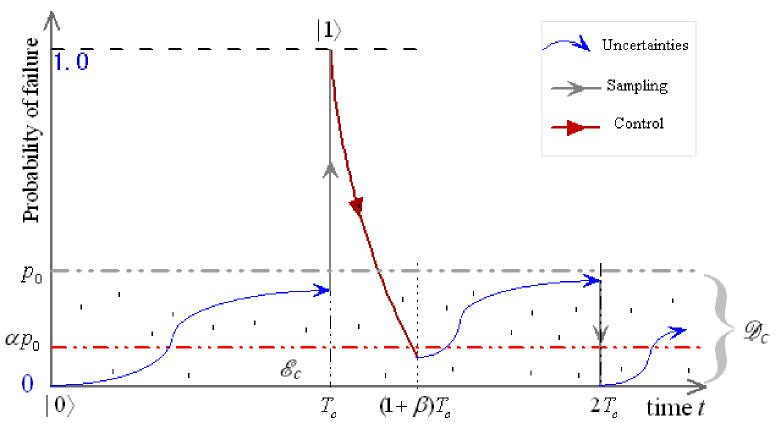
Figure 1: The proposed sampled-data control scheme for a single qubit system without decoherence. The labels “Control”, “Sampling” and “Uncertainties” refer to the evolution process under the unitary control, the sampling process, and uncertainties in the system Hamiltonian, respectively.

Using a similar argument to Theorem 1 in [29], we have the following result [30].

Lemma 5

For a single qubit with initial state $|\psi(0)\rangle=|0\rangle$ at time $t=0$, the system evolves to $|\psi(t)\rangle$ under the action of $H(t)=[1+\omega(t)]I_{z}+\epsilon_{x}(t)I_{x}+\epsilon_{y}(t)I_{y}$ (where $|\omega(t)|\leq\omega$, $\omega\geq 0$, $\sqrt{\epsilon_{x}^{2}(t)+\epsilon_{y}^{2}(t)}\leq\epsilon$ and $\epsilon>0$). If $t\in[0,T_{c}]$, where

$$T_{c}=\frac{\arccos(1-2p_{0})}{\epsilon},$$ (9)

the state will remain in $\mathcal{D}_{c}=\{|\psi\rangle:|\langle 0|\psi\rangle|^{2}\geq 1-p_{0}\}$ (where $0<p_{0}<1$). When a projective measurement is made with the operator $\sigma_{z}$ at time $t$, the probability of failure $p=|\langle 1|\psi(t)\rangle|^{2}$ is not greater than $p_{0}$.

We use $T_{c}$ defined in (9) as the sampling period to guarantee the required performance. If the sampling data corresponds to $|1\rangle$, a unitary control is required to drive the state back to a subset $\mathcal{E}_{c}$ of $\mathcal{D}_{c}$. The following theorem gives a sufficient condition on the relationships between $\alpha$, $p_{0}$ and $\beta$ to guarantee the required robustness.

Theorem 6

For a single qubit with initial state $|\psi(0)\rangle$ satisfying $|\langle\psi(0)|1\rangle|^{2}$ $\leq\alpha p_{0}$ ($0\leq\alpha\leq 1$) at time $t=0$, the system evolves to $|\psi(t)\rangle$ under the action of $H(t)=[1+\omega(t)]I_{z}+\epsilon_{x}(t)I_{x}+\epsilon_{y}(t)I_{y}$ (where $\sqrt{\epsilon_{x}^{2}(t)+\epsilon_{y}^{2}(t)}\leq\epsilon$, $\epsilon>0$, $|\omega(t)|\leq\omega$ and $\omega\geq 0$). If $t\in[0,(1-\beta)T_{c}]$ and

$$\alpha\leq\frac{1-\cos[\beta\arccos(1-2p_{0})]}{2p_{0}}$$ (10)

where $0\leq\beta<1$ and

$$T_{c}=\frac{\arccos(1-2p_{0})}{\epsilon},$$ (11)

then the state will remain in $\mathcal{D}_{c}=\{|\psi\rangle:|\langle 0|\psi\rangle|^{2}\geq 1-p_{0}\}$ (where $0<p_{0}<1$). When a projective measurement is made with the operator $\sigma_{z}$ at time $t$, the probability of failure $p=|\langle 1|\psi(t)\rangle|^{2}$ is not greater than $p_{0}$.

Remark 2

Using Lemma 5 and Theorem 6, we aim to maintain the state in $\mathcal{D}_{c}$ by implementing periodic sampling with period $T_{c}$ in (9). This theorem provides a sufficient condition to guarantee the required robustness. Given $p_{0}$, $\beta$, we can select $\alpha$ satisfying (10) in Theorem 6. If the sampled result is $|1\rangle$, we apply a unitary control to drive the state into $\mathcal{E}_{c}$. The sampling period and the unitary control can be designed in advance. Different approaches can be used to design such a unitary control law. In this paper, we will employ a Lyapunov method [60]-[63] in Example 2 to accomplish this task for the closed quantum system.

Remark 3

The design scheme above involves a sampling process and a unitary control. It is similar to the approach used in [29]. The difference lies in the fact that the scheme in this paper involves a fixed sampling period $T_{c}$. However, the approach in [29] involves at least two measurement periods $T$ (equivalent to $T_{c}$ in this paper) and $T_{1}$ ($T_{1}\ll T$). This situation means that the approach of [29] may require measurements which are very close together, which may be difficult to achieve in practice. In this sense, the sampled-data design in this paper is more practical than the method in [29].

III-B Amplitude damping decoherence

For single qubit systems with amplitude damping decoherence, if the initial state is excited state $|0\rangle$, the decoherence will drive this excited state to the ground state $|1\rangle$. The objective is to design a control law to guarantee the required robustness defined by $\mathcal{D}_{a}$. We use a similar sampled-data design method to that in the case without decoherence. That is, if the state is $|0\rangle$ at $t=nT_{a}$ ($n=0,1,2,\dots$), we design a sampling period to maintain the system’s state in $\mathcal{D}_{a}$ by implementing periodic sampling with period $T_{a}$; if the measurement makes the state collapse into $|1\rangle$ (with a probability $p\leq p_{0}$), we design a unitary control to drive the state back into a subset $\mathcal{E}_{a}$ of $\mathcal{D}_{a}$ from $t=nT_{a}$ to $(n+\beta)T_{a}$, and then sample again at $t=(n+1)T_{a}$. In order to determine the required sampling period, we have the following results.

Theorem 7

For a single qubit with initial state $|0\rangle$ at time $t=0$, the system evolves to $\rho(t)$ subject to (6) where $H(t)=[1+\omega(t)]I_{z}+\epsilon_{x}(t)I_{x}+\epsilon_{y}(t)I_{y}$ ($\sqrt{\epsilon_{x}^{2}(t)+\epsilon_{y}^{2}(t)}\leq\epsilon$, $\epsilon>0$, $|\omega(t)|\leq\omega$ and $\omega\geq 0$) and the coupling strength of amplitude damping decoherence is $\gamma_{t}=\gamma_{0}+\delta\gamma_{t}$ ($|\delta\gamma_{t}|\leq\gamma$). If $t\in[0,T_{a}]$ with

$$T_{a}=\frac{2p_{0}}{\sqrt{4\epsilon^{2}+(\gamma_{0}+\gamma)^{2}}+(\gamma_{0}+\gamma)},$$ (12)

the state will remain in $\mathcal{D}_{a}=\{\rho:\langle 0|\rho|0\rangle\geq 1-p_{0}\}$ (where $0<p_{0}<1$). When a projective measurement is made with the operator $\sigma_{z}$ at time $t$, the probability of failure $p=\langle 1|\rho|1\rangle$ is not greater than $p_{0}$.

Corollary 8

If $p_{0}\leq\frac{1}{2}-\frac{\gamma_{0}+\gamma}{2\sqrt{4\epsilon^{2}+(\gamma_{0}+\gamma)^{2}}}$ and $t\in[0,T_{a}^{\prime}]$, the sampling period $T_{a}$ in (12) can be replaced by $T_{a}^{\prime}$ to guarantee the same robustness as in Theorem 7, where

$$T_{a}^{\prime}=\frac{2p_{0}}{4\epsilon\sqrt{p_{0}-p_{0}^{2}}+2(\gamma_{0}+\gamma)(1-p_{0})}.$$ (13)

When there exist no uncertainties in the system Hamiltonian (i.e., $H_{\Delta}\equiv 0$), the sampling period can be designed using the following proposition.

Proposition 9

For a single qubit with initial state $|0\rangle$ at time $t=0$, the system evolves to $\rho(t)$ subject to (6) where $H(t)=I_{z}$ and the coupling strength of amplitude damping decoherence is $\gamma_{t}=\gamma_{0}+\delta\gamma_{t}$ ($|\delta\gamma_{t}|\leq\gamma$). If $t\in[0,T_{a}^{\prime\prime}]$ with

$$T_{a}^{\prime\prime}=-\frac{\ln(1-p_{0})}{\gamma_{0}+\gamma},$$ (14)

the state will remain in $\mathcal{D}_{a}=\{\rho:\langle 0|\rho|0\rangle\geq 1-p_{0}\}$ (where $0<p_{0}<1$). When a projective measurement is made with the operator $\sigma_{z}$ at time $t$, the probability of failure $p=\langle 1|\rho|1\rangle$ is not greater than $p_{0}$.

Remark 4

From the proof of Proposition 9, it is clear that $T_{a}^{\prime\prime}=-\frac{\ln(1-p_{0})}{\gamma_{0}+\gamma}$ exactly corresponds to the case $\delta\gamma_{t}\equiv\gamma$ when $H_{\Delta}\equiv 0$. In this sense, the sampling period $T_{a}^{\prime\prime}=-\frac{\ln(1-p_{0})}{\gamma_{0}+\gamma}$ is optimal to guarantee the required robustness. From the proofs of Theorem 7 and Corollary 8, it is clear that $T_{a}^{\prime}\geq T_{a}$. The relationship $T_{a}^{\prime\prime}\geq T_{a}$ for arbitrary $p_{0}$ can be proved by the following steps: (a) Define $F(p_{0})=T_{a}^{\prime\prime}-T_{a}$; (b) observe $F(p_{0}=0)=0$; and (c) verify $\frac{\text{d}F}{\text{d}p_{0}}\geq 0$.

Hence, for different situations we may use $T_{a}$, $T_{a}^{\prime}$ or $T_{a}^{\prime\prime}$ as the sampling period to guarantee the required performance. If the sampled data corresponds to $|1\rangle$, a unitary control is required to drive the state back to a subset $\mathcal{E}_{a}$ of $\mathcal{D}_{a}$. The subset $\mathcal{E}_{a}$ may be defined as $\mathcal{E}_{a}=\{\rho:\langle 0|\rho|0\rangle\geq 1-\alpha p_{0},0<p_{0}<1,0\leq\alpha\leq 1\}$. The following theorem gives a sufficient condition on the relationships between $\alpha$, $p_{0}$ and $\beta$ to guarantee the required robustness (The following conclusion is also true when $T_{a}$ can be replaced by $T_{a}^{\prime}$ or $T_{a}^{\prime\prime}$).

Theorem 10

For a single qubit with initial state $\rho(0)$ satisfying $\langle 1|\rho(0)|1\rangle$ $\leq\alpha p_{0}$ ($0\leq\alpha\leq 1$) at time $t=0$, the system evolves to $\rho(t)$ subject to (6) where $H(t)=[1+\omega(t)]I_{z}+\epsilon_{x}(t)I_{x}+\epsilon_{y}(t)I_{y}$ ($\sqrt{\epsilon_{x}^{2}(t)+\epsilon_{y}^{2}(t)}\leq\epsilon$, $\epsilon>0$, $|\omega(t)|\leq\omega$ and $\omega\geq 0$) and the coupling strength of amplitude damping decoherence is $\gamma_{t}=\gamma_{0}+\delta\gamma_{t}$ ($|\delta\gamma_{t}|\leq\gamma$). If $t\in[0,(1-\beta)T_{a}]$ and

$$\alpha\leq\beta$$ (15)

where $0<\beta\leq 1$ and

$$T_{a}=\frac{2p_{0}}{\sqrt{4\epsilon^{2}+(\gamma_{0}+\gamma)^{2}}+(\gamma_{0}+\gamma)},$$ (16)

the state will remain in $\mathcal{D}_{a}=\{\rho:\langle 0|\rho|0\rangle\geq 1-p_{0}\}$ (where $0<p_{0}<1$). When a projective measurement is made with the operator $\sigma_{z}$ at time $t$, the probability of failure $p=\langle 1|\rho|1\rangle$ is not greater than $p_{0}$.

III-C Phase damping decoherence

For a single qubit with phase damping decoherence, we define the coherence as $C=x^{2}+y^{2}$ where $x=\text{tr}(\rho\sigma_{x})$ and $y=\text{tr}(\rho\sigma_{y})$. The phase damping decoherence will reduce the coherence of the system. The objective is to guarantee that the state has coherence not less than $\bar{C}$ by periodic sampling when there exist uncertainties in the coupling strength of system-environment interaction and in the system Hamiltonian. To determine the required sampling period, we have the following results.

Theorem 11

For a single qubit with initial state $\rho_{0}$ satisfying $C_{0}=[\text{tr}(\rho_{0}\sigma_{x})]^{2}+[\text{tr}(\rho_{0}\sigma_{y})]^{2}=1$ at time $t=0$, the system evolves to $\rho_{t}$ subject to (7) where $H(t)=[1+\omega(t)]I_{z}+\epsilon_{x}(t)I_{x}+\epsilon_{y}(t)I_{y}$ ($\sqrt{\epsilon_{x}^{2}(t)+\epsilon_{y}^{2}(t)}\leq\epsilon$, $\epsilon>0$, $|\omega(t)|\leq\omega$ and $\omega\geq 0$) and the coupling strength of the phase damping decoherence is $\gamma_{t}=\gamma_{0}+\delta\gamma_{t}$ ($|\delta\gamma_{t}|\leq\gamma$). If $t\in[0,T_{p}]$ with

$$T_{p}=\begin{cases}\frac{1-\bar{C}}{4\sqrt{2}(\gamma_{0}+\gamma)},\ \ \ \text{when}\ 4(\gamma_{0}+\gamma)^{2}\geq\epsilon^{2};\\ \frac{(1-\bar{C})\sqrt{\epsilon^{2}-2(\gamma_{0}+\gamma)^{2}}}{2\epsilon^{2}},\ \ \ \text{when}\ 4(\gamma_{0}+\gamma)^{2}<\epsilon^{2},\end{cases}$$ (17)

the state will remain in $\mathcal{D}_{p}=\{\rho_{t}:[\text{tr}(\rho_{t}\sigma_{x})]^{2}+[\text{tr}(\rho_{t}\sigma_{y})]^{2}\geq\bar{C},0<\bar{C}\leq 1\}$. When a periodic projective measurement is made with the operator $\sigma_{x}$ on the system, the sampling (measurement) period $T_{p}$ can guarantee that the state remains in $\mathcal{D}_{p}$.

Corollary 12

When $\epsilon^{2}=2(\gamma_{0}+\gamma)^{2}$, the sampling period $T_{p}$ in (17) can be replaced by $T_{p}^{\prime}$ to guarantee the same robustness as in Theorem 11, where

$$T_{p}^{\prime}=\frac{1-\sqrt{\bar{C}}}{2\sqrt{2}(\gamma_{0}+\gamma)}.$$ (18)

If $H_{\Delta}\equiv 0$, we can design the sampling period using the following proposition.

Proposition 13

For a single qubit with initial state $\rho_{0}$ satisfying $C_{0}=[\text{tr}(\rho_{0}\sigma_{x})]^{2}+[\text{tr}(\rho_{0}\sigma_{y})]^{2}=1$ at time $t=0$, the system evolves to $\rho(t)$ subject to (7) where $H(t)=I_{z}$ and the coupling strength of the phase damping decoherence is $\gamma_{t}=\gamma_{0}+\delta\gamma_{t}$ ($|\delta\gamma_{t}|\leq\gamma$). If $t\in[0,T_{p}^{\prime\prime}]$ with

$$T_{p}^{\prime\prime}=-\frac{\ln\bar{C}}{4(\gamma_{0}+\gamma)},$$ (19)

the state will remain in $\mathcal{D}_{p}=\{\rho_{t}:[\text{tr}(\rho_{t}\sigma_{x})]^{2}+[\text{tr}(\rho_{t}\sigma_{y})]^{2}\geq\bar{C},0<\bar{C}\leq 1\}$. If a periodic projective measurement is made with the operator $\sigma_{x}$, the sampling period $T_{p}^{\prime\prime}$ can guarantee that the system’s state remains in $\mathcal{D}_{p}$.

Remark 5

For $2(\gamma+\gamma_{0})^{2}=\epsilon^{2}$, it is straightforward to prove that $T_{p}^{\prime}\geq T_{p}$. The relationship $T_{p}^{\prime\prime}\geq T_{p}$ can be proved by the following steps: (a) Denote $Y=1-\bar{C}$; (b) define $F(Y)=T_{p}^{\prime\prime}-T_{p}$; (c) observe $F(Y=0)=0$; and (d) verify $\frac{\text{d}F(Y)}{\text{d}Y}\geq 0$. From the proof of Proposition 13, it is clear that the sampling period $T_{p}^{\prime\prime}$ is optimal to guarantee the required robustness when $H_{\Delta}\equiv 0$. For this case with phase damping decoherence, we can also make projective measurements with the operator $\sigma_{y}$, which does not affect the conclusions. Moreover, in this case, no unitary control is required and measurement is the only tool needed for guaranteeing the required robustness. It is worth mentioning that several methods based only on measurements have recently been proposed for controlling quantum systems (see, e.g., [64]-[67]).

Remark 6

We can also consider a class of imperfect measurements. This class of uncertainties may arise from precision limitations of the measurement apparatus or from system errors in the measurement device. Measurement with the operator $\sigma_{z}$ will make the system collapse into $|0\rangle$ or $|1\rangle$ (eigenstates of $H_{0}$). We consider the imperfect measurement model shown as in Fig. 2. $p_{01}$ is the error probability of measurement from $|0\rangle$ to $|1\rangle$, that is, the probability that one obtains the result $|1\rangle$ when making a measurement on the system in $|0\rangle$; $p_{10}$ is the error probability of measurement from $|1\rangle$ to $|0\rangle$, where $0\leq p_{01}<1$ and $0\leq p_{10}<1$. This class of imperfect measurements does not affect the effectiveness of the sampled-data design. Thus, the proposed method can tolerate this additional uncertainty in the sampling process.

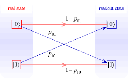
Figure 2: The model for imperfect measurement. $p_{01}$ is the error probability of measurement from $|0\rangle$ to $|1\rangle$ and $p_{10}$ is the error probability of measurement from $|1\rangle$ to $|0\rangle$.

III-D Depolarizing decoherence

For a single qubit, the depolarizing decoherence will reduce the purity $P=\text{tr}(\rho^{2})$ of the system’s state. The objective is to guarantee that the purity of the state is not less than $\bar{P}$ by periodic sampling when there exist uncertainties in the coupling strength of system-environment interaction and in the system Hamiltonian. To determine the required sampling period, we have the following results.

Theorem 14

For a single qubit with initial state $\rho_{0}$ satisfying $\text{tr}(\rho_{0}^{2})=1$ at time $t=0$, the system evolves to $\rho_{t}$ subject to (8) where $H(t)=[1+\omega(t)]I_{z}+\epsilon_{x}(t)I_{x}+\epsilon_{y}(t)I_{y}$ ($\sqrt{\epsilon_{x}^{2}(t)+\epsilon_{y}^{2}(t)}\leq\epsilon$, $\epsilon>0$, $|\omega(t)|\leq\omega$ and $\omega\geq 0$) and the coupling strength of depolarizing decoherence is $\gamma_{t}=\gamma_{0}+\delta\gamma_{t}$ ($|\delta\gamma_{t}|\leq\gamma$). If $t\in[0,T_{d}]$ with

$$T_{d}=-\frac{\ln(2\bar{P}-1)}{8(\gamma_{0}+\gamma)},$$ (20)

the state will remain in $\mathcal{D}_{d}=\{\rho_{t}:\text{tr}(\rho_{t}^{2})\geq\bar{P},0.5<\bar{P}\leq 1\}$. If periodic projective measurements are made with the operator $\sigma_{z}$, the sampling period $T_{d}$ can guarantee that the state remains in $\mathcal{D}_{d}$.

Remark 7

The selection of measurement operators (i.e., $\sigma_{x}$, $\sigma_{y}$ or $\sigma_{z}$), uncertainties in the system Hamiltonian ($H_{\Delta}\neq 0$ or $H_{\Delta}\equiv 0$) and the imperfect measurement described in Fig. 2 do not affect the conclusion in Theorem 14. The sampling period $T_{d}$ is also optimal to guarantee the required robustness.

The sampling periods for the different cases considered above are summarized in Table 1.

Table 1: Summary of sampling periods for different cases. $H_{\Delta}(x,y,z)=\omega(t)I_{z}+\epsilon_{x}(t)I_{x}+\epsilon_{y}(t)I_{y}$ (where $\sqrt{\epsilon_{x}^{2}(t)+\epsilon_{y}^{2}(t)}\leq\epsilon$, $\epsilon>0$, $|\omega(t)|\leq\omega$ and $\omega\geq 0$), $f(\epsilon,\gamma_{0},\gamma)=\frac{1}{2}-\frac{\gamma_{0}+\gamma}{2\sqrt{4\epsilon^{2}+(\gamma_{0}+\gamma)^{2}}}$, and coupling strength $\gamma_{t}=\gamma_{0}+\delta\gamma_{t}$ ($|\delta\gamma_{t}|\leq\gamma$). $H_{\Delta}(x,y,z)$ is also considered for the two cases $p_{0}\leq f(\epsilon,\gamma_{0},\gamma)$ and $\epsilon^{2}=2(\gamma_{0}+\gamma)^{2}$. The parameters values $p_{0}=0.01$, $\gamma_{0}=0.9$, $\gamma=0.1$ and $\bar{C}=\bar{P}=0.95$ are assumed for the calculation of the right two columns. When $4(\gamma_{0}+\gamma)^{2}\geq\epsilon^{2}$, $\overline{T}=\frac{1-\bar{C}}{4\sqrt{2}(\gamma_{0}+\gamma)}$; when $4(\gamma_{0}+\gamma)^{2}<\epsilon^{2}$, $\overline{T}=\frac{(1-\bar{C})\sqrt{\epsilon^{2}-2(\gamma_{0}+\gamma)^{2}}}{2\epsilon^{2}}$.

cases		sampling period	$\epsilon=0.2$	$\epsilon=\sqrt{2}$
closed system with $H_{\Delta}(x,y,z)$		$T_{c}=\frac{\arccos(1-2p_{0})}{\epsilon}$	$T_{c}=1.0017$	$T_{c}=0.1417$
amplitude	$H_{\Delta}(x,y,z)$	$T_{a}=\frac{2p_{0}}{\sqrt{4\epsilon^{2}+(\gamma_{0}+\gamma)^{2}}+(\gamma_{0}+\gamma)}$	$T_{a}=0.0096$	$T_{a}=0.0050$
damping	$p_{0}\leq f(\epsilon,\gamma_{0},\gamma)$	$T_{a}^{\prime}=\frac{2p_{0}}{4\epsilon\sqrt{p_{0}-p_{0}^{2}}+2(\gamma_{0}+\gamma)(1-p_{0})}$	$-$	$T_{a}^{\prime}=0.0079$
decoherence	$H_{\Delta}\equiv 0$	$T_{a}^{\prime\prime}=-\frac{\ln(1-p_{0})}{\gamma_{0}+\gamma}$	$T_{a}^{\prime\prime}=0.0101$	$T_{a}^{\prime\prime}=0.0101$
phase	$H_{\Delta}(x,y,z)$	$T_{p}=\overline{T}$	$T_{p}=0.0088$	$T_{p}=0.0088$
damping	$\epsilon^{2}=2(\gamma_{0}+\gamma)^{2}$	$T_{p}^{\prime}=\frac{1-\sqrt{\bar{C}}}{2\sqrt{2}(\gamma_{0}+\gamma)}$	$-$	$T_{p}^{\prime}=0.0090$
decoherence	$H_{\Delta}\equiv 0$	$T_{p}^{\prime\prime}=-\frac{\ln\bar{C}}{4(\gamma_{0}+\gamma)}$	$T_{p}^{\prime\prime}=0.0128$	$T_{p}^{\prime\prime}=0.0128$
depolarizing	$H_{\Delta}(x,y,z)$	$T_{d}=-\frac{\ln(2\bar{P}-1)}{8(\gamma_{0}+\gamma)}$	$T_{d}=0.0131$	$T_{d}=0.0131$
decoherence	$H_{\Delta}\equiv 0$	$T_{d}=-\frac{\ln(2\bar{P}-1)}{8(\gamma_{0}+\gamma)}$	$T_{d}=0.0131$	$T_{d}=0.0131$

III-E Illustrative examples

Example 1 (Sampling periods)

The values of sampling periods are shown in the right two columns of Table 1 for several specific cases, where we have assumed $p_{0}=0.01$, $\gamma_{0}=0.9$, $\gamma=0.1$ and $\bar{C}=\bar{P}=0.95$. Further, we can consider a real quantum system of a superconducting box in [2], [68]. Let the resonance frequency $\tilde{\omega}_{0}=2\pi\times 100\text{MHz}$ and the cavity decay rate $\tilde{\gamma}_{0}=2\pi\times 0.8\text{MHz}$. Assume that $\tilde{\gamma}=\frac{2\pi\times 0.8\text{MHz}}{9}$ and $\tilde{\epsilon}=2\pi\times 1.0\text{MHz}$. Hence, the cavity decay time $T_{\gamma}=198.9\text{ns}$. Using the results in Table 1, we can get the real sampling periods as $\tilde{T}_{c}=8.0\text{ns}$, $\tilde{T}_{a}=1.0\text{ns}$, $\tilde{T}_{a}^{\prime\prime}=1.8\text{ns}$, $\tilde{T}_{p}=1.6\text{ns}$, $\tilde{T}_{p}^{\prime\prime}=2.3\text{ns}$ and $\tilde{T}_{d}=2.5\text{ns}$.

Example 2 (Unitary control for Case A))

Theorem 6 gives a sufficient condition for designing a unitary control to guarantee the required robustness. Here we employ a Lyapunov method [60]-[62] to design such a unitary control where the Lyapunov function is constructed based on the Hilbert-Schmidt distance between a state $|\psi\rangle$ and the sliding mode state $|0\rangle$; i.e., $V(|\psi\rangle,|0\rangle)=\frac{1}{2}(1-|\langle 0|\psi\rangle|^{2}).$ The control values can be selected as (for details, see [29], [63]):

$$u_{k}=K_{k}f_{k}(\Im[e^{i\angle\langle\psi|\phi_{j}\rangle}\langle 0|I_{k}|\psi\rangle]),\ \ \ (k=x,y,z)$$ (21)

where $\Im[a+bi]=b$ ($a,b\in\mathbf{R}$). Here $\angle c$ denotes the argument of a complex number $c$, the parameter $K_{k}>0$ may be used to adjust the control amplitude, and $f(\cdot)$ satisfies $xf(x)\geq 0$. We define $\angle\langle\psi|0\rangle=0^{\circ}$ when $\langle\psi|0\rangle=0$ and adopt the parameter values of $p_{0}=0.01$, $\epsilon=0.2$ and $\beta=0.05$. From the simulation in [29], we find that the Lyapunov control is not sensitive to small uncertainties in the system Hamiltonian. Additional simulation results suggest that the robustness of the Lyapunov control can be enhanced if we choose the terminal condition $|\langle 1|\psi(t)\rangle|^{2}\leq\eta\alpha p_{0}$ (where $0<\eta<1$) instead of $|\langle 1|\psi(t)\rangle|^{2}\leq\alpha p_{0}$. Here, we select $\eta=0.8$. Hence, we design the sampling period $T_{c}=1.0017$ using (9). Using Theorem 6, we select $\alpha=2.5\times 10^{-3}$. We design the Lyapunov control using (21) and the terminal condition $|\langle 1|\psi(t)\rangle|^{2}\leq\eta\alpha p_{0}=2.0\times 10^{-5}$ with the control Hamiltonian $H_{u}=\frac{1}{2}u(t)\sigma_{y}$. Using (21), we select $u(t)=K(\Im[e^{i\angle\langle\psi(t)|0\rangle}\langle 0|\sigma_{y}|\psi(t)\rangle])$, $K=500$, and let the time stepsize be $\delta t=10^{-6}$. We obtain the probability curve for $|0\rangle$ shown in Fig. 3(a) and the control value shown in Fig. 3(b). For the noise $\epsilon(t)I_{x}$ or $\epsilon(t)I_{y}$ where $\epsilon(t)$ is a uniform distribution in $[-0.2,0.2]$, additional simulation results show that the state is also driven into $\mathcal{E}_{c}$ using the Lyapunov control in Fig. 3(b).

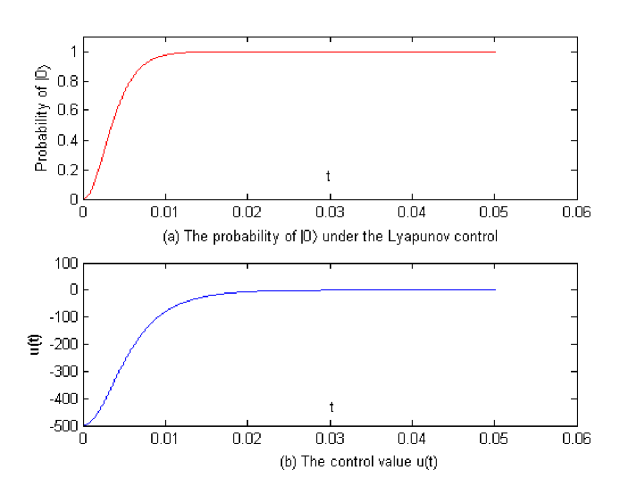
Figure 3: The probability of $|0\rangle$ and the control value $u(t)$ under the Lyapunov control.

Example 3 (Unitary control for Case B))

For amplitude damping decoherence, Theorem 10 gives a sufficient condition for designing a unitary control to guarantee the required robustness. Here, we employ a constant control $H_{u}=\frac{1}{2}u\sigma_{y}$ ($u=6466$), and assume $p_{0}=0.01$, $\epsilon=0.2$, $\gamma_{0}=0.9$ and $\beta=0.05$. Using Theorem 10, we may select $\alpha=0.05$. Let the time stepsize be $\delta t=10^{-7}$. The curve for $z_{t}=\text{tr}(\rho_{t}\sigma_{z})$ is shown in Fig. 4.

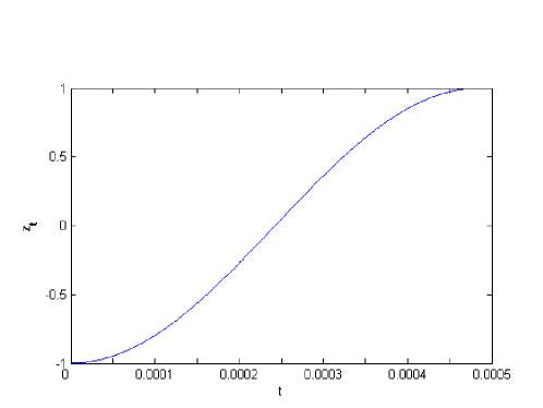
Figure 4: The curve of $z_{t}$ for the case with amplitude damping decoherence, where $H_{u}=3233\sigma_{y}$.

Remark 8

The required unitary control can be designed using strategies such as the Lyapunov method and optimal control theory. In Example 2 and Example 3, we used simulation to find appropriate control amplitudes for achieving the required objectives. Additional simulation experiments also show that $u(t)$ can tolerate small uncertainties. Since it is necessary to drive the state back to a subset of the sliding mode domain within a small time period, the required control amplitudes generally are relatively large, which is similar to the case of decoherence control based on dynamical decoupling [24], [47]. The selection of small $\beta$ makes it reasonable that we first design the unitary control by ignoring possible uncertainties and then verify the robustness of the unitary control to uncertainties by simulation. Here, we present only simulated examples to demonstrate how such a unitary control can be designed. A systematic investigation into the design of the unitary control and finding optimal control amplitudes that can tolerate uncertainties will be the subject of future work.

IV Proof of the Main Results

IV-A Proof of Theorem 6

To prove Theorem 6, we first prove two lemmas (Lemma 15 and Lemma 16). Lemma 15 compares the probabilities of failure for $H(t)=[1+\omega(t)]I_{z}+\epsilon\cos\phi_{0}I_{y}+\epsilon\sin\phi_{0}I_{x}$ and $H(t)=\epsilon\cos\phi_{0}I_{y}+\epsilon\sin\phi_{0}I_{x}$. Lemma 15 together with Lemma 16 demonstrates that $H=\epsilon I_{x}$ can be used to estimate an upper bound on the probability of failure for $H(t)=[1+\omega(t)]I_{z}+\epsilon_{x}(t)I_{x}+\epsilon_{y}(t)I_{y}$ when $z_{0}=1$.

Lemma 15

For a single qubit with initial state $(x_{0},y_{0},z_{0})=(0,0,1)$, the system evolves to $(x^{A}_{t},y^{A}_{t},z^{A}_{t})$ and $(x^{B}_{t},y^{B}_{t},z^{B}_{t})$ under the action of $H^{A}=[1+\omega(t)]I_{z}+\epsilon\cos\phi_{0}I_{y}+\epsilon\sin\phi_{0}I_{x}$ (with constant $\epsilon>0$ and $|\omega(t)|\leq\omega$) and $H^{B}=\epsilon\cos\phi_{0}I_{y}+\epsilon\sin\phi_{0}I_{x}$, respectively. For arbitrary $t\in[0,\frac{\pi}{2\sqrt{4+\epsilon^{2}}}]$, $z^{A}_{t}\geq z^{B}_{t}$.

Proof:

For the system with Hamiltonian $H^{A}=[1+\omega(t)]I_{z}+\epsilon\cos\phi_{0}I_{y}+\epsilon\sin\phi_{0}I_{x}$, using (4) and (5), we obtain the following state equations

$$\left(\begin{array}[]{c}\dot{x}_{t}^{A}\\ \dot{y}_{t}^{A}\\ \dot{z}_{t}^{A}\\ \end{array}\right)=\left(\begin{array}[]{ccc}0&-[1+\omega(t)]&\epsilon\cos\phi_{0}\\ 1+\omega(t)&0&-\epsilon\sin\phi_{0}\\ -\epsilon\cos\phi_{0}&\epsilon\sin\phi_{0}&0\\ \end{array}\right)\left(\begin{array}[]{c}x_{t}^{A}\\ y_{t}^{A}\\ z_{t}^{A}\\ \end{array}\right),$$ (22)

where $(x_{0}^{A},y_{0}^{A},z_{0}^{A})=(0,0,1)$.

Consider $\omega(t)$ as a control input and select the performance measure as

$$J(\omega)=z_{f}.$$ (23)

We introduce the Lagrange multiplier vector $\lambda(t)=(\lambda_{1}(t),\lambda_{2}(t),\lambda_{3}(t))^{T}$ and obtain the corresponding Hamiltonian function as follows:

$$\mathbb{H}({\mathbf{r}(t),\omega(t),\mathbf{\lambda}(t),t})\equiv\lambda^{T}(t)\left(\begin{array}[]{ccc}0&-[1+\omega(t)]&\epsilon\cos\phi_{0}\\ 1+\omega(t)&0&-\epsilon\sin\phi_{0}\\ -\epsilon\cos\phi_{0}&\epsilon\sin\phi_{0}&0\\ \end{array}\right)\left(\begin{array}[]{c}x_{t}\\ y_{t}\\ z_{t}\\ \end{array}\right),$$ (24)

where $\mathbf{r}(t)=(x_{t},y_{t},z_{t})$. That is

$$\begin{array}[]{c}\mathbb{H}({\mathbf{r}(t),\omega(t),\mathbf{\lambda}(t),t})\\ =[1+\omega(t)](\lambda_{2}(t)x_{t}-\lambda_{1}(t)y_{t})+\epsilon\cos\phi_{0}(\lambda_{1}(t)z_{t}-\lambda_{3}(t)x_{t})-\epsilon\sin\phi_{0}(\lambda_{2}(t)z_{t}-\lambda_{3}(t)y_{t}).\end{array}$$ (25)

According to Pontryagin’s minimum principle [69], a necessary condition for $\omega^{*}(t)$ to minimize $J(\omega)$ is

$$\mathbb{H}({\mathbf{r}^{*}(t),\omega^{*}(t),\mathbf{\lambda}^{*}(t),t})\leq\mathbb{H}({\mathbf{r}^{*}(t),\omega(t),\mathbf{\lambda}^{*}(t),t}).$$ (26)

Hence, if we do not consider singular cases (i.e., $\lambda_{2}(t)x_{t}-\lambda_{1}(t)y_{t}\equiv 0$), the optimal control $\omega^{*}(t)$ should be chosen as follows:

$$\omega^{*}(t)=-\omega\text{sgn}(\lambda_{2}(t)x_{t}-\lambda_{1}(t)y_{t}).$$ (27)

That is, the optimal control strategy for $\omega(t)$ is bang-bang control; i.e., $\omega^{*}(t)=\bar{\omega}=+\omega\ \text{or}-\omega$. Now we consider $H^{A}=(1+\bar{\omega})I_{z}+\epsilon\cos\phi_{0}I_{y}+\epsilon\sin\phi_{0}I_{x}$, which leads to the following state equations

$$\left(\begin{array}[]{c}\dot{x}_{t}^{A}\\ \dot{y}_{t}^{A}\\ \dot{z}_{t}^{A}\\ \end{array}\right)=\left(\begin{array}[]{ccc}0&-(1+\bar{\omega})&\epsilon\cos\phi_{0}\\ 1+\bar{\omega}&0&-\epsilon\sin\phi_{0}\\ -\epsilon\cos\phi_{0}&\epsilon\sin\phi_{0}&0\\ \end{array}\right)\left(\begin{array}[]{c}x_{t}^{A}\\ y_{t}^{A}\\ z_{t}^{A}\\ \end{array}\right),$$ (28)

where $(x_{0}^{A},y_{0}^{A},z_{0}^{A})=(0,0,1)$. The corresponding solution is

$$\left(\begin{array}[]{c}x_{t}^{A}\\ y_{t}^{A}\\ z_{t}^{A}\\ \end{array}\right)=\\ \left(\begin{array}[]{c}\frac{\epsilon\cos\phi_{0}}{\sqrt{(1+\bar{\omega})^{2}+\epsilon^{2}}}\sin\upsilon t-\frac{(1+\bar{\omega})\epsilon\sin\phi_{0}}{(1+\bar{\omega})^{2}+\epsilon^{2}}\cos\upsilon t+\frac{(1+\bar{\omega})\epsilon\sin\phi_{0}}{(1+\bar{\omega})^{2}+\epsilon^{2}}\\ -\frac{\epsilon\sin\phi_{0}}{\sqrt{(1+\bar{\omega})^{2}+\epsilon^{2}}}\sin\upsilon t-\frac{(1+\bar{\omega})\epsilon\cos\phi_{0}}{(1+\bar{\omega})^{2}+\epsilon^{2}}\cos\upsilon t+\frac{(1+\bar{\omega})\epsilon\cos\phi_{0}}{(1+\bar{\omega})^{2}+\epsilon^{2}}\\ \frac{\epsilon^{2}}{(1+\bar{\omega})^{2}+\epsilon^{2}}\cos\upsilon t+\frac{(1+\bar{\omega})^{2}}{(1+\bar{\omega})^{2}+\epsilon^{2}}\\ \end{array}\right),$$ (29)

where $\upsilon=\sqrt{(1+\bar{\omega})^{2}+\epsilon^{2}}$. From (29), we know that $z_{t}$ is a monotonically decreasing function in $t$ when $t\in[0,\frac{\pi}{2\sqrt{4+\epsilon^{2}}}]$. Hence, we only consider the case $t\in[0,t_{f}]$ where $t_{f}\in[0,\frac{\pi}{2\sqrt{4+\epsilon^{2}}}]$.

Now consider the optimal control problem with a fixed final time $t_{f}$ and a free final state $\mathbf{r}_{f}=(x_{f},y_{f},z_{f})$. According to Pontryagin’s minimum principle, $\lambda^{*}(t_{f})=\frac{\partial}{\partial\mathbf{r}}\mathbf{r}^{*}(t_{f})$, and it is straightforward to verify that $(\lambda_{1}(t_{f}),\lambda_{2}(t_{f}),\lambda_{3}(t_{f}))=(0,0,1)$. Now consider another necessary condition $\dot{\lambda}(t)=-\frac{\partial\mathbb{H}({\mathbf{r}(t),\epsilon(t),\mathbf{\lambda}(t),t})}{\partial\mathbf{r}}$ which leads to the following relationships:

$$\dot{\mathbf{\lambda}}(t)=\left(\begin{array}[]{c}\dot{\lambda}_{1}(t)\\ \dot{\lambda}_{2}(t)\\ \dot{\lambda}_{3}(t)\\ \end{array}\right)=\left(\begin{array}[]{ccc}0&-(1+\bar{\omega})&\epsilon\cos\phi_{0}\\ 1+\bar{\omega}&0&-\epsilon\sin\phi_{0}\\ -\epsilon\cos\phi_{0}&\epsilon\sin\phi_{0}&0\\ \end{array}\right)\left(\begin{array}[]{c}\lambda_{1}(t)\\ \lambda_{2}(t)\\ \lambda_{3}(t)\\ \end{array}\right),$$ (30)

where $(\lambda_{1}(t_{f}),\lambda_{2}(t_{f}),\lambda_{3}(t_{f}))=(0,0,1)$. The corresponding solution is

$$\left(\begin{array}[]{c}\lambda_{1}(t)\\ \lambda_{2}(t)\\ \lambda_{3}(t)\\ \end{array}\right)=\left(\begin{array}[]{c}-\frac{\epsilon\cos\phi_{0}}{\sqrt{(1+\bar{\omega})^{2}+\epsilon^{2}}}\sin\upsilon(t_{f}-t)-\frac{(1+\bar{\omega})\epsilon\sin\phi_{0}}{(1+\bar{\omega})^{2}+\epsilon^{2}}\cos\upsilon(t_{f}-t)+\frac{(1+\bar{\omega})\epsilon\sin\phi_{0}}{(1+\bar{\omega})^{2}+\epsilon^{2}}\\ \frac{\epsilon\sin\phi_{0}}{\sqrt{(1+\bar{\omega})^{2}+\epsilon^{2}}}\sin\upsilon(t_{f}-t)-\frac{(1+\bar{\omega})\epsilon\cos\phi_{0}}{(1+\bar{\omega})^{2}+\epsilon^{2}}\cos\upsilon(t_{f}-t)+\frac{(1+\bar{\omega})\epsilon\cos\phi_{0}}{(1+\bar{\omega})^{2}+\epsilon^{2}}\\ \frac{\epsilon^{2}}{(1+\bar{\omega})^{2}+\epsilon^{2}}\cos\upsilon(t_{f}-t)+\frac{(1+\bar{\omega})^{2}}{(1+\bar{\omega})^{2}+\epsilon^{2}}\\ \end{array}\right).$$ (31)

We obtain

$$\lambda_{2}(t)x_{t}-\lambda_{1}(t)y_{t}=\frac{\epsilon^{2}(1+\bar{\omega})}{\upsilon^{3/2}}[\sin\upsilon t+\sin\upsilon(t_{f}-t)-\sin\upsilon t_{f}].$$ (32)

It is easy to show that the quantity $(\lambda_{2}(t)x_{t}-\lambda_{1}(t)y_{t})\geq 0$ occurring in (27) does not change sign when $t_{f}\in[0,\frac{\pi}{2\sqrt{4+\epsilon^{2}}}]$ and $t\in[0,t_{f}]$. Hence, the optimal control is $\delta^{*}(t)=\bar{\omega}=-\omega$.

We now exclude the possibility that there exists a singular case. Suppose that there exists a singular interval $[t_{0},t_{1}]$ (where $t_{0}\geq 0$ and we assume that $[t_{0},t_{1}]$ is the first singular interval) such that when $t\in[t_{0},t_{1}]$

$$h(t)=\lambda_{2}(t)x_{t}-\lambda_{1}(t)y_{t}\equiv 0.$$ (33)

We also have the following relationship

$$\ddot{h}(t)=\lambda_{3}(t)x_{t}-\lambda_{1}(t)z_{t}\equiv 0$$ (34)

where we have used (22) and the following costate equation

$$\dot{\mathbf{\lambda}}(t)=\left(\begin{array}[]{c}\dot{\lambda}_{1}(t)\\ \dot{\lambda}_{2}(t)\\ \dot{\lambda}_{3}(t)\\ \end{array}\right)=\left(\begin{array}[]{ccc}0&-[1+\omega(t)]&\epsilon\cos\phi_{0}\\ 1+\omega(t)&0&-\epsilon\sin\phi_{0}\\ -\epsilon\cos\phi_{0}&\epsilon\sin\phi_{0}&0\\ \end{array}\right)\left(\begin{array}[]{c}\lambda_{1}(t)\\ \lambda_{2}(t)\\ \lambda_{3}(t)\\ \end{array}\right).$$ (35)

If $t_{0}=0$, we have $(x_{0},y_{0},z_{0})=(0,0,1)$. By the principle of optimality [69], we may consider the case $t_{f}=t_{1}$. Using (33), (34) and $(\lambda_{1}(t_{1}),\lambda_{2}(t_{1}),\lambda_{3}(t_{1}))=(0,0,1)$, we have $x_{t_{1}}=0$ and $y_{t_{1}}=0$. Using the relationship of $x^{2}_{t}+y^{2}_{t}+z_{t}^{2}=1$, we obtain $z_{t_{1}}=1$ or $-1$. If $z_{t_{1}}=1$, the initial and final states are the same state $|0\rangle$. However, if we use the control $\omega(t)=\bar{\omega}$, from (29) we have $z_{t_{1}}(\bar{\omega})=\frac{\epsilon^{2}}{(1+\bar{\omega})^{2}+\epsilon^{2}}\cos\upsilon t_{1}+\frac{(1+\bar{\omega})^{2}}{(1+\bar{\omega})^{2}+\epsilon^{2}}<z_{t_{1}}=1$. Hence, this contradicts the fact that we are considering the optimal case $\min z_{f}$. If $z_{t_{1}}=-1$, there exists $0<\tilde{t}_{1}<t_{1}$ such that $z_{\tilde{t}_{1}}=0$. By the principle of optimality [69], we may consider the case $t_{f}=\tilde{t}_{1}$. From the two equations (33) and (34), we know that $z^{2}_{\tilde{t}_{1}}=1$ which contradicts $z_{\tilde{t}_{1}}=0$. Hence, no singular condition can exist if $t_{0}=0$.

If $t_{0}>0$, using (27) we must select $\omega(t)=\bar{\omega}$ when $t\in[0,t_{0}]$. From (32), we know that there exist no $t_{0}\in(0,t_{f})$ satisfying $\lambda_{2}(t_{0})x_{t_{0}}-\lambda_{1}(t_{0})y_{t_{0}}=0$. Hence, there exist no singular cases for our problem. From the previous analysis, $\omega(t)=-\omega$ is the optimal control when $t\in[0,\frac{\pi}{2\sqrt{4+\epsilon^{2}}}]$.

For the system with Hamiltonian $H^{B}=\epsilon\cos\phi_{0}I_{y}+\epsilon\sin\phi_{0}I_{x}$, using (4) and (5), we obtain the following state equations

$$\left(\begin{array}[]{c}\dot{x}_{t}^{B}\\ \dot{y}_{t}^{B}\\ \dot{z}_{t}^{B}\\ \end{array}\right)=\left(\begin{array}[]{ccc}0&0&\epsilon\cos\phi_{0}\\ 0&0&-\epsilon\sin\phi_{0}\\ -\epsilon\cos\phi_{0}&\epsilon\sin\phi_{0}&0\\ \end{array}\right)\left(\begin{array}[]{c}x_{t}^{B}\\ y_{t}^{B}\\ z_{t}^{B}\\ \end{array}\right),$$ (36)

where $(x_{0}^{B},y_{0}^{B},z_{0}^{B})=(0,0,1)$. The corresponding solution is

$$\left(\begin{array}[]{c}x_{t}^{B}\\ y_{t}^{B}\\ z_{t}^{B}\\ \end{array}\right)=\\ \left(\begin{array}[]{c}\cos\phi_{0}\sin\epsilon t\\ -\sin\phi_{0}\sin\epsilon t\\ \cos\epsilon t\\ \end{array}\right).$$ (37)

We define $F(t)$ and $f(t)$ as follows:

$$F(t)=z_{t}^{A}-z_{t}^{B}=\frac{\epsilon^{2}}{(1-\omega)^{2}+\epsilon^{2}}\cos\upsilon t+\frac{(1-\omega)^{2}}{(1-\omega)^{2}+\epsilon^{2}}-\cos\epsilon t,$$ (38)

$$f(t)=\dot{F}(t)=-\frac{\epsilon^{2}}{\sqrt{(1-\omega)^{2}+\epsilon^{2}}}\sin\upsilon t+\epsilon\sin\epsilon t.$$ (39)

Now, consider $t\in[0,\frac{\pi}{2\sqrt{4+\epsilon^{2}}}]$ to obtain

$$\dot{f}(t)=\epsilon^{2}(\cos\epsilon t-\cos\upsilon t)\geq 0.$$ (40)

It is clear that $\dot{f}(t)=0$ only when $t=0$. Hence $f(t)$ is a monotonically increasing function and

$$\min_{t}{f(t)}=f(0)=0.$$

Hence, we have

$$f(t)\geq 0.$$ (41)

From this result, it is clear that $F(t)$ is a monotonically increasing function and

$$\min_{t}{F(t)}=F(0)=0.$$

Hence $F(t)\geq 0$ when $t\in[0,\frac{\pi}{2\sqrt{4+\epsilon^{2}}}]$. Therefore, we can conclude that $z^{A}_{t}\geq z^{B}_{t}$ for arbitrary $t\in[0,\frac{\pi}{2\sqrt{4+\epsilon^{2}}}]$. ∎

We now present another lemma.

Lemma 16

For a single qubit with initial state $(x_{0},y_{0},z_{0})=(0,0,1)$, suppose that the system evolves to $(x_{t},y_{t},z_{t})$ under the action of $H=\epsilon(\cos\phi I_{y}+\sin\phi I_{x})$ ($\phi$ is a constant). Then, $z_{t}$ is independent of $\phi$.

Proof:

For $H=\omega(\sin\phi I_{x}+\cos\phi I_{y})$, from (37), we have

$$z_{t}=\cos\epsilon t.$$

It is clear that $z_{t}$ is independent of $\phi$. ∎

Remark 9

Since $z_{t}$ is independent of $\phi$, it is enough to consider a special case $\phi=\frac{\pi}{2}$ when analyzing $z_{t}$ under $H=\epsilon(\cos\phi I_{y}+\sin\phi I_{x})$.

Now we can prove Theorem 6.

Proof:

For a single qubit, assume that the state at time $t$ is $\rho_{t}$. If we make a measurement with the operator $\sigma_{z}$, the probability $p$ that the state will collapse into $|1\rangle$ (the probability of failure) is

$$p=\langle 1|\rho_{t}|1\rangle=\frac{1-z_{t}}{2}.$$ (42)

For a closed single qubit system, its state $|\psi\rangle$ can be represented as

$$|\psi\rangle=\cos{\frac{\theta}{2}}|0\rangle+e^{i\varphi}\sin{\frac{\theta}{2}}|1\rangle,$$ (43)

where its bloch vector corresponds to $(x,y,z)=(\sin\theta\cos\varphi,\sin\theta\sin\varphi,\cos\theta)$, $\theta\in[0,\pi]$, $\varphi\in[0,2\pi]$.

For $H^{A}=[1+\omega(t)]I_{z}+\epsilon_{x}(t)I_{x}+\epsilon_{y}(t)I_{y}$, using $\dot{\rho}=-i[H^{A},\rho]$ and (4), we obtain the following state equations

$$\left(\begin{array}[]{c}\dot{x}_{t}^{A}\\ \dot{y}_{t}^{A}\\ \dot{z}_{t}^{A}\\ \end{array}\right)=\left(\begin{array}[]{ccc}0&-[1+\omega(t)]&\epsilon_{y}(t)\\ 1+\omega(t)&0&-\epsilon_{x}(t)\\ -\epsilon_{y}(t)&\epsilon_{x}(t)&0\\ \end{array}\right)\left(\begin{array}[]{c}x_{t}^{A}\\ y_{t}^{A}\\ z_{t}^{A}\\ \end{array}\right).$$ (44)

Define $\epsilon(t)=\sqrt{\epsilon_{x}^{2}(t)+\epsilon_{y}^{2}(t)}$ and $\epsilon_{x}(t)=\epsilon(t)\sin\phi_{t}$ , $\epsilon_{y}(t)=\epsilon(t)\cos\phi_{t}$. This leads to the following equation

$$\left(\begin{array}[]{c}\dot{x}_{t}^{A}\\ \dot{y}_{t}^{A}\\ \dot{z}_{t}^{A}\\ \end{array}\right)=\left(\begin{array}[]{ccc}0&-[1+\omega(t)]&\epsilon(t)\cos\phi_{t}\\ 1+\omega(t)&0&-\epsilon(t)\sin\phi_{t}\\ -\epsilon(t)\cos\phi_{t}&\epsilon(t)\sin\phi_{t}&0\\ \end{array}\right)\left(\begin{array}[]{c}x_{t}^{A}\\ y_{t}^{A}\\ z_{t}^{A}\\ \end{array}\right).$$ (45)

For $H^{B}=\epsilon I_{x}$, we have

$$\left(\begin{array}[]{c}\dot{x}_{t}^{B}\\ \dot{y}_{t}^{B}\\ \dot{z}_{t}^{B}\\ \end{array}\right)=\left(\begin{array}[]{ccc}0&0&0\\ 0&0&-\epsilon\\ 0&\epsilon&0\\ \end{array}\right)\left(\begin{array}[]{c}x_{t}^{B}\\ y_{t}^{B}\\ z_{t}^{B}\\ \end{array}\right).$$ (46)

When $(x_{0}^{A},y_{0}^{A},z_{0}^{A})=(x_{0}^{B},y_{0}^{B},z_{0}^{B})=(0,0,1)$, for $\Delta t\rightarrow 0$, we have from Lemma 15 and Lemma 16

$$z_{\Delta t}^{A}\geq z_{\Delta t}^{B}.$$ (47)

We will now prove that the relationship $z_{\Delta t}^{A}\geq z_{\Delta t}^{B}$ ($\Delta t\rightarrow 0$) is also true for $z_{0}^{A}=z_{0}^{B}=\cos\theta_{0}$ (where $\theta_{0}\in(0,\pi)$). We assume that there exist $\tilde{t}\in(0,\Delta t]$ such that

$$z_{\tilde{t}}^{A}<z_{\tilde{t}}^{B}.$$ (48)

Define $f(t)=z_{t}^{A}-z_{t}^{B}$. Since $f(t)$ is continuous in $t$ and $f(0)=0$, there exists a time $t^{*}=\sup\{t|0\leq t<\tilde{t},f(t)=0\}$ satisfying $f(t^{*})=0$ and $f(t)<0$ for $t\in(t^{*},\tilde{t}]$. Hence

$$\dot{f}(t)|_{t=t^{*}}\leq 0.$$ (49)

Let $z_{t^{*}}^{A}=z_{t^{*}}^{B}=\cos\theta^{*}$. We can assume $(x_{t^{*}}^{A},y_{t^{*}}^{A},z_{t^{*}}^{A})=(\sin\theta^{*}\cos\varphi^{*},\sin\theta^{*}\sin\varphi^{*},\cos\theta^{*})$ and $(x_{t^{*}}^{B},y_{t^{*}}^{B},z_{t^{*}}^{B})=(0,-\sin\theta^{*},\cos\theta^{*})$ (where $\varphi^{*}\in[0,2\pi]$). Define $N(t)=-\epsilon(t)\sin\theta^{*}\cos(\phi_{t}+\varphi^{*})$. From (45) and (46), we have

$$\dot{f}(t)|_{t=t^{*}}=\dot{z}_{t}^{A}|_{t=t^{*}}-\dot{z}^{B}_{t}|_{t=t^{*}}=\lim_{t\rightarrow t^{*}}N(t)+\epsilon\sin\theta^{*}.$$ (50)

For arbitrary $t$, it is clear that

$$N(t)\geq-\epsilon\sin\theta^{*}.$$ (51)

When $N(t)>-\epsilon\sin\theta^{*}$, $\dot{f}(t)|_{t=t^{*}}>0$, which contradicts (49). When $N(t)=-\epsilon\sin\theta^{*}$, since $\sin\theta^{*}\neq 0$, we have $\epsilon(t^{*})=\epsilon$ and $\phi_{t^{*}}=2\pi-\varphi^{*}$. Using Pontryagin’s minimum principle [69] and a similar argument in Lemma 15 and Lemma 16, we can prove $z^{A}_{t^{*}+\Delta t}\geq z^{B}_{t^{*}+\Delta t}$. Hence we can conclude that for $z_{0}^{A}=z_{0}^{B}=\cos\theta_{0}$ (where $\theta_{0}\in[0,\pi)$) and $\Delta t\rightarrow 0$,

$$z^{A}_{\Delta t}\geq z^{B}_{\Delta t}.$$ (52)

From (46), we know that $z^{B}_{t}=\cos(\theta_{0}+\epsilon t)$. When $0<t<\frac{\pi-\theta_{0}}{\epsilon}$, $z^{B}_{t}$ decreases monotonically in $t$. We now define $g(t)=z^{A}_{t}-z^{B}_{t}$ and assume that there exist $t=t_{1}\in[0,\frac{\pi-\theta_{0}}{\epsilon})$ such that $z^{A}_{t_{1}}<z^{B}_{t_{1}}$. That is, $g(t_{1})<0$. Since $g(t)$ is continuous in $t$ and $g(0)=0$, there exists a time $t^{*}=\sup\{t|0\leq t<t_{1},g(t)=0\}$ satisfying $g(t)<0$ for $t\in(t^{*},t_{1}]$. However, we have established that for any $z_{t}^{A}=z_{t}^{B}$ and $\Delta t\rightarrow 0$, $z_{t+\Delta t}^{A}\geq z_{t+\Delta t}^{B}$, which contradicts $g(t)<0$ for $t\in(t^{*},t_{1}]$. Hence, we have the following relationship for $t\in[0,\frac{\pi-\theta_{0}}{\epsilon})$

$$z^{A}_{t}\geq z^{B}_{t}.$$ (53)

From (42), it is clear that the probabilities of failure satisfy $p^{A}_{t}=\frac{1-z^{A}_{t}}{2}\leq p^{B}_{t}=\frac{1-z^{B}_{t}}{2}$. That is, the probability of failure $p_{t}^{A}$ is not greater than $p^{B}_{t}$ for $t\in[0,\frac{\pi-\theta_{0}}{\epsilon})$.

Since $z_{t}^{B}=\cos(\theta_{0}+\epsilon t)$, we have $\Delta z^{B}_{\beta T_{c}}=\cos\theta_{0}-\cos(\theta_{0}+\epsilon\beta T)$, where

$$T_{c}=\frac{\arccos(1-2p_{0})}{\epsilon}.$$ (54)

When $|\langle\psi(0)|1\rangle|^{2}\leq\alpha p_{0}$, using the previous argument, we have

$$z^{A}_{\beta T_{c}}\geq 1-2\alpha p_{0}+\cos(\theta_{0}+\epsilon\beta T_{c})-\cos\theta_{0}=M.$$

Now let

$$p=\frac{1-z^{A}_{\beta T_{c}}}{2}\leq\frac{1-M}{2}\leq p_{0}.$$

Using the fact $\theta_{0}=\arccos(1-2\alpha p_{0})$, we have the following relationship

$$\alpha\leq\frac{1-\cos[(1-\beta)\arccos(1-2p_{0})]}{2p_{0}}.$$ (55)

∎

IV-B Proof of Theorem 7

Proof:

For the open qubit system subject to (6), when $H(t)=[1+\omega(t)]I_{z}+\epsilon_{x}(t)I_{x}+\epsilon_{y}(t)I_{y}$ ($\sqrt{\epsilon_{x}^{2}(t)+\epsilon_{y}^{2}(t)}\leq\epsilon$, $\epsilon>0$, $|\omega(t)|\leq\omega$ and $\omega\geq 0$), $\gamma_{t}=\gamma_{0}+\delta\gamma_{t}$ ($|\delta\gamma_{t}|\leq\gamma$), using (4), we have

$$\left(\begin{array}[]{c}\dot{x}_{t}\\ \dot{y}_{t}\\ \dot{z}_{t}\\ \end{array}\right)=\left(\begin{array}[]{ccc}-\frac{1}{2}(\gamma_{0}+\delta\gamma_{t})&-(1+\omega(t))&\epsilon_{y}(t)\\ 1+\omega(t)&-\frac{1}{2}(\gamma_{0}+\delta\gamma_{t})&-\epsilon_{x}(t)\\ -\epsilon_{y}(t)&\epsilon_{x}(t)&-(\gamma_{0}+\delta\gamma_{t})\\ \end{array}\right)\left(\begin{array}[]{c}x_{t}\\ y_{t}\\ z_{t}\\ \end{array}\right)+\left(\begin{array}[]{c}0\\ 0\\ -(\gamma_{0}+\delta\gamma_{t})\\ \end{array}\right),$$ (56)

where $(x_{0},y_{0},z_{0})=(0,0,1)$. From (56), we have

$$\begin{array}[]{cc}\dot{z_{t}}&=-\epsilon_{y}(t)x_{t}+\epsilon_{x}(t)y_{t}-(\gamma_{0}+\delta\gamma_{t})(z_{t}+1)\\ &\geq-2\epsilon\sqrt{1-z_{t}^{2}}-(\gamma_{0}+\gamma)(z_{t}+1).\end{array}$$ (57)

Denoting

$$f(z)=2\epsilon\sqrt{1-z_{t}^{2}}+(\gamma_{0}+\gamma)(1+z_{t}),$$ (58)

we have

$$\frac{\text{d}f(z)}{\text{d}z}=(\gamma_{0}+\gamma)-2\epsilon\frac{z_{t}}{\sqrt{1-z_{t}^{2}}}.$$ (59)

Let $\frac{\text{d}f(z)}{\text{d}z}=0$ to find the solution $z=\frac{\gamma_{0}+\gamma}{\sqrt{4\epsilon^{2}+(\gamma_{0}+\gamma)^{2}}}$. Hence,

$$\max f(z)=f(\frac{\gamma_{0}+\gamma}{\sqrt{4\epsilon^{2}+(\gamma_{0}+\gamma)^{2}}})=\sqrt{4\epsilon^{2}+(\gamma_{0}+\gamma)^{2}}+(\gamma_{0}+\gamma).$$ (60)

Hence,

$$\dot{z_{t}}\geq-\max f(z)=-\sqrt{4\epsilon^{2}+(\gamma_{0}+\gamma)^{2}}-(\gamma_{0}+\gamma).$$ (61)

When $t\in[0,T_{a}]$ where

$$T_{a}=\frac{2p_{0}}{\sqrt{4\epsilon^{2}+(\gamma_{0}+\gamma)^{2}}+(\gamma_{0}+\gamma)},$$ (62)

we have

$$z_{t}\geq 1-(\max f(z))t\geq 1-2p_{0}.$$ (63)

Therefore, if one makes a measurement on the system with $\sigma_{z}$, the probability of failure $\langle 1|\rho_{t}|1\rangle=\frac{1-z_{t}}{2}\leq p_{0}$. ∎

IV-C Proof of Corollary 8

Proof:

When $p_{0}\leq\frac{1}{2}-\frac{\gamma_{0}+\gamma}{2\sqrt{4\epsilon^{2}+(\gamma_{0}+\gamma)^{2}}}$, from the proof of Theorem 7, we know for $z\in[1-2p_{0},1]$,

$$\max f(z)=f(1-2p_{0})=4\epsilon\sqrt{p_{0}-p_{0}^{2}}+2(\gamma_{0}+\gamma)(1-p_{0}).$$ (64)

Hence, if $t\in[0,T_{a}^{\prime}]$ where

$$T_{a}^{\prime}=\frac{2p_{0}}{4\epsilon\sqrt{p_{0}-p_{0}^{2}}+2(\gamma_{0}+\gamma)(1-p_{0})},$$ (65)

$$z_{t}\geq 1-[4\epsilon\sqrt{p_{0}-p_{0}^{2}}+2(\gamma_{0}+\gamma)(1-p_{0})]t\geq 1-2p_{0}.$$ (66)

It is clear that the probability of failure $\langle 1|\rho_{t}|1\rangle\leq p_{0}$. ∎

IV-D Proof of Proposition 9

Proof:

When $H(t)=I_{z}$ and $\gamma_{t}=\gamma_{0}+\delta\gamma_{t}$, the state equation of the system in (6) is

$$\left(\begin{array}[]{c}\dot{x}_{t}\\ \dot{y}_{t}\\ \dot{z}_{t}\\ \end{array}\right)=\left(\begin{array}[]{ccc}-\frac{1}{2}(\gamma_{0}+\delta\gamma_{t})&-1&0\\ 1&-\frac{1}{2}(\gamma_{0}+\delta\gamma_{t})&0\\ 0&0&-(\gamma_{0}+\delta\gamma_{t})\\ \end{array}\right)\left(\begin{array}[]{c}x_{t}\\ y_{t}\\ z_{t}\\ \end{array}\right)+\left(\begin{array}[]{c}0\\ 0\\ -(\gamma_{0}+\delta\gamma_{t})\\ \end{array}\right),$$ (67)

where $(x_{0},y_{0},z_{0})=(0,0,1)$. It is clear that

$$\dot{z_{t}}=-(\gamma_{0}+\delta\gamma_{t})(1+z_{t})\geq-(\gamma_{0}+\gamma)(1+z_{t}).$$ (68)

From (68), we have

$$z_{t}\geq 2e^{-(\gamma_{0}+\gamma)t}-1.$$ (69)

If $t\in[0,T_{a}^{\prime\prime}]$ where

$$T_{a}^{\prime\prime}=-\frac{\ln(1-p_{0})}{\gamma_{0}+\gamma},$$ (70)

we have

$$z_{t}\geq 1-2p_{0}.$$ (71)

That is, the probability of failure $\langle 1|\rho_{t}|1\rangle\leq p_{0}$. ∎

IV-E Proof of Theorem 10

Proof:

From the proof of Theorem 7, we know

$$\dot{z_{t}}\geq-\max f(z)=-\sqrt{4\epsilon^{2}+(\gamma_{0}+\gamma)^{2}}-(\gamma_{0}+\gamma).$$

Now if the initial state $z_{0}\geq 1-2\alpha p_{0}$ and $t\in[0,(1-\beta)T_{a}]$, the system’s state satisfies

$$z_{t}\geq z_{0}-(\sqrt{4\epsilon^{2}+(\gamma_{0}+\gamma)^{2}}+(\gamma_{0}+\gamma))(1-\beta)T_{a}\geq 1-2(1+\alpha-\beta)p_{0}.$$ (72)

When $\alpha\leq\beta$, we have the following relationship

$$z_{t}\geq 1-2p_{0}.$$ (73)

Hence, the probability of failure satisfies $\langle 1|\rho_{t}|1\rangle\leq p_{0}$. ∎

IV-F Proof of Theorem 11

Proof:

For a single qubit subject to (7) when $H(t)=[1+\omega(t)]I_{z}+\epsilon_{x}(t)I_{x}+\epsilon_{y}(t)I_{y}$ ($|\omega(t)|\leq\omega$, $\sqrt{\epsilon_{x}^{2}(t)+\epsilon_{y}^{2}(t)}\leq\epsilon$, $\omega\geq 0$ and $\epsilon>0$), $\gamma_{t}=\gamma_{0}+\delta\gamma_{t}$ ($|\delta\gamma_{t}|\leq\gamma$), using (4), we have

$$\left(\begin{array}[]{c}\dot{x}_{t}\\ \dot{y}_{t}\\ \dot{z}_{t}\\ \end{array}\right)=\left(\begin{array}[]{ccc}-2(\gamma_{0}+\delta\gamma_{t})&-(1+\omega(t))&\epsilon_{y}(t)\\ 1+\omega(t)&-2(\gamma_{0}+\delta\gamma_{t})&-\epsilon_{x}(t)\\ -\epsilon_{y}(t)&\epsilon_{x}(t)&0\\ \end{array}\right)\left(\begin{array}[]{c}x_{t}\\ y_{t}\\ z_{t}\\ \end{array}\right),$$ (74)

where $C_{0}=x_{0}^{2}+y_{0}^{2}=1$. Let $C_{t}=x_{t}^{2}+y_{t}^{2}$. We have

$$\begin{array}[]{cc}\dot{C_{t}}&=2x_{t}\dot{x}_{t}+2y_{t}\dot{y}_{t}=-4(\gamma_{0}+\delta\gamma_{t})(x_{t}^{2}+y_{t}^{2})+2z_{t}(\epsilon_{y}(t)x_{t}-\epsilon_{x}(t)y_{t})\\ &\geq-4(\gamma_{0}+\delta\gamma_{t})(x_{t}^{2}+y_{t}^{2})-2\epsilon\sqrt{1-(x_{t}^{2}+y_{t}^{2})}(|x_{t}|+|y_{t}|)\\ &\geq-4(\gamma_{0}+\delta\gamma_{t})(x_{t}^{2}+y_{t}^{2})-2\epsilon\sqrt{1-(x_{t}^{2}+y_{t}^{2})}\sqrt{2(x_{t}^{2}+y_{t}^{2})}\end{array}$$ (75)

Let $N_{t}=2(\gamma_{0}+\gamma)^{2}C_{t}^{2}-\epsilon^{2}C_{t}^{2}+\epsilon^{2}C_{t}$. We have

$$2(\gamma_{0}+\delta\gamma_{t})C_{t}+\epsilon\sqrt{2C_{t}(1-C_{t})}\leq\sqrt{2}\sqrt{4(\gamma_{0}+\delta\gamma_{t})^{2}C_{t}^{2}+2\epsilon^{2}C_{t}(1-C_{t})}\leq 2\sqrt{N_{t}}$$ (76)

Hence, $\dot{C_{t}}\geq-4\sqrt{\max N_{t}}$. According to the definition of $N_{t}$, it is easy to verify the fact

$$\max N_{t}=\begin{cases}2(\gamma_{0}+\gamma)^{2},\ \ \ \text{when}\ 4(\gamma_{0}+\gamma)^{2}\geq\epsilon^{2};\\ \frac{\epsilon^{4}}{4\epsilon^{2}-8(\gamma_{0}+\gamma)^{2}},\ \ \ \text{when}\ 4(\gamma_{0}+\gamma)^{2}<\epsilon^{2}.\end{cases}$$ (77)

If $t\in[0,T_{p}]$ where

$$T_{p}=\begin{cases}\frac{1-\bar{C}}{4\sqrt{2}(\gamma_{0}+\gamma)},\ \ \ \text{when}\ 4(\gamma_{0}+\gamma)^{2}\geq\epsilon^{2};\\ \frac{(1-\bar{C})\sqrt{\epsilon^{2}-2(\gamma_{0}+\gamma)^{2}}}{2\epsilon^{2}},\ \ \ \text{when}\ 4(\gamma_{0}+\gamma)^{2}<\epsilon^{2},\end{cases}$$ (78)

we have $C_{t}\geq\bar{C}$.

∎

IV-G Proof of Corollary 12

Proof:

When $\epsilon^{2}=2(\gamma_{0}+\gamma)^{2}$, from (75) and (76), we have

$$\dot{C_{t}}\geq-4\sqrt{\epsilon^{2}C_{t}}.$$ (79)

It is easy to obtain the following relationship

$$2\text{d}\sqrt{C_{t}}\geq-4\epsilon\text{d}t,$$ (80)

$$\sqrt{C_{t}}\geq 1-2\epsilon t.$$ (81)

If $t\in[0,T_{p}^{\prime}]$ where

$$T_{p}^{\prime}=\frac{1-\sqrt{\bar{C}}}{2\sqrt{2}(\gamma_{0}+\gamma)},$$ (82)

we have $C_{t}\geq\bar{C}.$ ∎

IV-H Proof of Proposition 13

Proof:

When $H(t)=I_{z}$ and $\gamma_{t}=\gamma_{0}+\delta\gamma_{t}$, using (4) and (7), we have

$$\left(\begin{array}[]{c}\dot{x}_{t}\\ \dot{y}_{t}\\ \dot{z}_{t}\\ \end{array}\right)=\left(\begin{array}[]{ccc}-2(\gamma_{0}+\delta\gamma_{t})&-1&0\\ 1&-2(\gamma_{0}+\delta\gamma_{t})&0\\ 0&0&0\\ \end{array}\right)\left(\begin{array}[]{c}x_{t}\\ y_{t}\\ z_{t}\\ \end{array}\right),$$ (83)

where $C_{0}=x_{0}^{2}+y_{0}^{2}=1$. It is clear that

$$\dot{C_{t}}=2x_{t}\dot{x}_{t}+2y_{t}\dot{y}_{t}=-4(\gamma_{0}+\delta\gamma_{t})(x_{t}^{2}+y_{t}^{2})\geq-4(\gamma_{0}+\gamma)C_{t}.$$ (84)

Hence,

$$C_{t}\geq e^{-4(\gamma_{0}+\gamma)t}.$$ (85)

If $t\in[0,T_{p}^{\prime\prime}]$ where

$$T_{p}^{\prime\prime}=-\frac{\ln\bar{C}}{4(\gamma_{0}+\gamma)},$$ (86)

we have $C_{t}\geq\bar{C}$. ∎

IV-I Proof of Theorem 14

Proof:

For a single qubit system subject to (8), when $H(t)=[1+\omega(t)]I_{z}+\epsilon_{x}(t)I_{x}+\epsilon_{y}(t)I_{y}$ ($\sqrt{\epsilon_{x}^{2}(t)+\epsilon_{y}^{2}(t)}\leq\epsilon$, $\epsilon>0$, $|\omega(t)|\leq\omega$ and $\omega\geq 0$), $\gamma_{t}=\gamma_{0}+\delta\gamma_{t}$ ($|\delta\gamma_{t}|\leq\gamma$), using (4), we have

$$\left(\begin{array}[]{c}\dot{x}_{t}\\ \dot{y}_{t}\\ \dot{z}_{t}\\ \end{array}\right)=\left(\begin{array}[]{ccc}-4(\gamma_{0}+\delta\gamma_{t})&-1&0\\ 1&-4(\gamma_{0}+\delta\gamma_{t})&0\\ 0&0&-4(\gamma_{0}+\delta\gamma_{t})\\ \end{array}\right)\left(\begin{array}[]{c}x_{t}\\ y_{t}\\ z_{t}\\ \end{array}\right),$$ (87)

where $P_{0}=x_{0}^{2}+y_{0}^{2}+z_{0}^{2}=1$ and $R_{t}=\text{tr}(\rho_{t}^{2})=x_{t}^{2}+y_{t}^{2}+z_{t}^{2}.$ It is clear that

$$\dot{R_{t}}=-8(\gamma_{0}+\delta\gamma_{t})P_{t}\geq-8(\gamma_{0}+\gamma)R_{t}.$$ (88)

Hence,

$$R_{t}\geq e^{-8(\gamma_{0}+\gamma)t}$$ (89)

If $t\in[0,T_{d}]$ where

$$T_{d}=-\frac{\ln(2\bar{P}-1)}{8(\gamma+\gamma_{0})},$$ (90)

we have $P_{t}\geq\bar{P}.$ ∎

V CONCLUSIONS

Control design for quantum systems with uncertainties is an important task. This paper has proposed a sampled-data design approach for a single qubit with uncertainties. Both closed and Markovian open quantum systems are investigated, and uncertainties in the system Hamiltonian and uncertainties in the coupling strength of the system-environment interaction are analyzed. Several physically meaningful performance indices including fidelity, coherence and purity are used to define the required robustness and several sufficient conditions on the relationships between related parameters in the control system are established to guarantee such robustness. The robust control law can be designed offline and then be used online on the single qubit system with uncertainties. Future work will include the extension of these sampled-data control approaches to other finite dimensional quantum systems and the development of practical applications of the proposed method.

References

- [1] D. Dong and I.R. Petersen, “Quantum control theory and applications: A survey,” IET Control Theory & Applications, Vol. 4, pp. 2651-2671, 2010.
- [2] H.M. Wiseman and G.J. Milburn, Quantum Measurement and Control, Cambridge, England: Cambridge University Press, 2010.
- [3] H. Rabitz, R. de Vivie-Riedle, M. Motzkus and K. Kompa, “Whither the future of controlling quantum phenomena?” Science, Vol. 288, pp. 824-828, 2000.
- [4] M.A. Nielsen and I.L. Chuang, Quantum Computation and Quantum Information, Cambridge, England: Cambridge University Press, 2000.
- [5] D. D’Alessandro, Introduction to Quantum Control and Dynamics, Chapman & Hall/CRC, 2007.
- [6] N. Khaneja, R. Brockett and S.J. Glaser, “Time optimal control in spin systems”, Physical Review A, Vol. 63, p. 032308, 2001.
- [7] D. D’Alessandro and M. Dahleh, “Optimal control of two-level quantum systems,” IEEE Transactions on Automatic Control, Vol. 46, pp. 866-876, 2001.
- [8] S. Grivopoulos and B. Bamieh, “Optimal population transfers in a quantum system for large transfer time,” IEEE Transactions on Automatic Control, Vol. 53, pp.980-992, 2008.
- [9] U. Boscain and P. Mason, “Time minimal trajectories for a spin 1/2 particle in a magnetic field”, Journal of Mathematical Physics, Vol. 47, p. 062101, 2006.
- [10] H.M. Wiseman and G.J. Milburn, “Quantum theory of optical feedback via homodyne detection”, Physical Review Letters, Vol. 70, No. 5, pp.548-551, 1993.
- [11] A.C. Doherty, S. Habib, K. Jacobs, H. Mabuchi and S.M. Tan, “Quantum feedback control and classical control theory”, Physical Review A, Vol. 62, p.012105, 2000.
- [12] R. van Handel, J.K. Stockton and H. Mabuchi, “Feedback control of quantum state reduction”, IEEE Transactions on Automatic Control, Vol. 50, No. 6, pp.768-780, 2005.
- [13] J. Zhang, R.B. Wu, C.W. Li and T.J. Tarn, “Protecting coherence and entanglement by quantum feedback controls”, IEEE Transactions on Automatic Control, Vol. 55, No. 3, pp.619-633, 2010.
- [14] B. Qi and L. Guo, “Is measurement-based feedback still better for quantum control systems? ” Systems & Control Letters, Vol. 59, pp.333-339, 2010.
- [15] C. Sayrin, I. Dotsenko, X. Zhou, B. Peaudecerf, T. Rybarczyk, S. Gleyzes, P. Rouchon, M. Mirrahimi, H. Amini, M. Brune, J.-M. Raimond and S. Haroche, “Real-time quantum feedback prepares and stabilizes photon number states” Nature, Vol. 477, pp.73-77, 2011.
- [16] G. Zhang and M.R. James, “Direct and indirect couplings in coherent feedback control of linear quantum systems”, IEEE Transactions on Automatic Control, Vol. 56, No. 7, pp.1535-1550, 2011.
- [17] A. I. Maalouf and I. R. Petersen, “Sampled-data LQG control for a class of linear quantum systems,” Systems & Control Letters, Vol. 61, pp.369-374, 2012.
- [18] C. Altafini, “Feedback stabilization of isospectral control systems on complex flag manifolds: Application to quantum ensembles,” IEEE Transactions on Automatic Control, Vol. 52, pp. 2019-2028, 2007.
- [19] M. Yanagisawa and H. Kimura, “Transfer function approach to quantum control-part I: Dynamics of quantum feedback systems”, IEEE Transactions on Automatic Control, Vol. 48, pp.2107-2120, 2003.
- [20] M. Mirrahimi and R. van Handel, “Stabilizing feedback controls for quantum systems”, SIAM Optimization and Control, Vol. 46, No. 2, pp.445-467, 2007.
- [21] M.A. Pravia, N. Boulant, J. Emerson, E.M. Fortunato, T.F. Havel, D.G. Cory and A. Farid, “Robust control of quantum information”, Journal of Chemical Physics, Vol. 119, pp. 9993-10001, 2003.
- [22] N. Yamamoto, and L. Bouten, “Quantum risk-sensitive estimation and robustness”, IEEE Transactions on Automatic Control, Vol. 54, pp. 92-107, 2009.
- [23] J.S. Li and N. Khaneja, “Ensemble control of Bloch equations,” IEEE Transactions on Automatic Control, vol. 54, pp.528-536, 2009.
- [24] L. Viola and E. Knill, “Robust dynamical decoupling of quantum systems with bounded controls”, Physical Review Letters, Vol. 90, p. 037901, 2003.
- [25] D. Dong, J. Lam and I.R. Petersen, “Robust incoherent control of qubit systems via switching and optimisation”, International Journal of Control, Vol. 83, pp. 206-217, 2010.
- [26] M.R. James, H.I. Nurdin and I.R. Petersen, “ control of linear quantum stochastic systems”, IEEE Transactions on Automatic Control, Vol. 53, pp. 1787-1803, 2008.
- [27] M.R. James, “Risk-sensitive optimal control of quantum systems”, Physical Review A, Vol. 69, p. 032108, 2004.
- [28] D. Dong and I.R. Petersen, “Sliding mode control of quantum systems”, New Journal of Physics, Vol. 11, p. 105033, 2009.
- [29] D. Dong and I.R. Petersen, “Sliding mode control of two-level quantum systems”, Automatica, Vol. 48, pp.725-735, 2012.
- [30] D. Dong and I.R. Petersen, “Notes on sliding mode control of two-level quantum systems”, Automatica, Vol. 48, pp.3089-3097, 2012.
- [31] V.I. Utkin, “Variable structure systems with sliding modes”, IEEE Transactions on Automatic Control, Vol. AC-22, No. 2, pp. 212-222, 1977.
- [32] D. Dong and I.R. Petersen, “Sampled-data control of two-level quantum systems based on sliding mode design”, Proc. of 50th IEEE CDC-ECC, Orlando, USA, December 12-15, 2011.
- [33] T. Chen and B. Francis, Optimal Sampled-Data Control Systems, London: Springer-Verlag, 1995.
- [34] R. Vilela Mendes and V.I. Man’ko, “Quantum control and the Strocchi map”, Physical Review A, Vol. 67, p.053404, 2003.
- [35] D. Dong, C. Zhang, H. Rabitz, A. Pechen and T.J. Tarn, “Incoherent control of locally controllable quantum systems,” Journal of Chemical Physics, Vol. 129, p. 154103, 2008.
- [36] R. Romano and D. D’Alessandro, “Environment-mediated control of a quantum system”, Physical Review Letters, Vol. 97, p.080402, 2006.
- [37] V.P. Belavkin, “Theory of the control of observable quantum systems”, Automatica and Remote Control, Vol. 44, pp.178-188, 1983.
- [38] L. Bouten, R. van Handel and M.R. James, “A discrete invitation to quantum filtering and feedback control”, SIAM Review, Vol. 51, pp.239-316, 2009.
- [39] B. Misra and E.C.G. Sudarshan, “The Zeno’s paradox in quantum theory”, Journal of Mathematical Physics, Vol. 18, pp.756-763, 1977.
- [40] W.M. Itano, D.J. Heinzen, J.J. Bollinger, and D.J. Wineland, “Quantum Zeno effect”, Physical Review A, Vol. 41, pp.2295-2300, 1990.
- [41] H.-P. Breuer and F. Petruccione, The Theory of Open Quantum Systems, (Oxford University Press, 2002, 1st edn).
- [42] G. Gordon, G. Kurizki and D.A. Lidar, “Optimal dynamical decoherence control of a qubit”, Physical Review Letters, Vol. 101, p.010403, 2008.
- [43] P. Zanardi and M. Rasetti, “Noiseless quantum codes”, Physical Review Letters, Vol. 79, pp.3306-3309, 1997.
- [44] D.A. Lidar, I.L. Chuang and K.B. Whaley, “Decoherence-free subspaces for quantum computation”, Physical Review Letters, Vol. 81, pp.2594-2597, 1999.
- [45] P.G. Kwiat, A.J. Berglund, J.B. Altepeter and A.G. White, “Experimental verification of decoherence-free subspaces”, Science, Vol. 290, pp.498-501, 2000.
- [46] E. Knill, R. Laflamme and L. Viola, “Theory of quantum error correction for general noise”, Physical Review Letters, Vol. 84, pp.2525-2528, 2000.
- [47] L. Viola, E. Knill, and S. Lloyd, “Dynamical decoupling of open quantum systems”, Physical Review Letters, Vol. 82, pp.2417-2421, 1999.
- [48] K. Khodjasteh, D.A. Lidar and L. Viola, “Arbitrarily accurate dynamical control in open quantum systems”, Physical Review Letters, Vol. 104, p.090501, 2010.
- [49] D. Vitali, P. Tombesi and G. J. Milburn, “Controlling the decoherence of a ‘meter’ via stroboscopic feedback”, Physical Review Letters, Vol. 79, pp.2442-2445, 1997.
- [50] V. Protopopescu, R. Perez, C. D’Helon and J. Schmulen, “Robust control of decoherence in realistic one-qubit quantum gates”, Journal of Physics A: Mathematical and General, Vol. 36, pp.2175-2189, 2003.
- [51] J. Zhang, C.W. Li, R.B. Wu, T.J. Tarn and X.S. Liu, “Maximal suppression of decoherence in Markovian quantum systems”, Journal of Physics A: Mathematical and General, 2005, Vol. 38, pp.6587-6601.
- [52] W. Cui, Z.R. Xi and Y. Pan, “Optimal decoherence control in non-Markovian open dissipative quantum systems”, Physical Review A, Vol. 77, p.032117, 2008.
- [53] G. Lindblad, “On the generators of quantum dynamical semigroups,” Communications in Mathematical Physics, 1976, Vol. 48, pp.119-130.
- [54] R. Alicki and K. Lendi, Quantum Dynamical Semigroups and Applications, (Springer, 2007, 2nd edn).
- [55] F. Ticozzi and L. Viola, “Quantum Markovian subsystems: invariance, attractivity, and control,” IEEE Transactions on Automatic Control, 2008, Vol. 53, pp.2048-2063.
- [56] S. Bolognani and F. Ticozzi, “Engineering stable discrete-time quantum dynamics via a canonical QR decomposition”, IEEE Transactions on Automatic Control, Vol. 55, pp.2721-2734, 2010.
- [57] F. Ticozzi and L. Viola, “Analysis and synthesis of attractive quantum Markovian dynamics”, Automatica, Vol. 45, pp.2002-2009, 2009.
- [58] D.A. Lidar and S. Schneider, “Stabilizing qubit coherence via tracking-control”, Quantum Information and Computation, Vol. 5, pp.350-363, 2005.
- [59] M. Zhang, H.Y. Dai, Z.R. Xi, H.W. Xie and D.W. Hu, “Combating dephasing decoherence by periodically performing tracking control and projective measurement”, Physical Review A, 2007, Vol. 76, p.042335.
- [60] M. Mirrahimi, P. Rouchon and G. Turinici, “Lyapunov control of bilinear Schrödinger equations”, Automatica, Vol. 41, pp. 1987-1994, 2005.
- [61] X. Wang and S.G. Schirmer, “Analysis of Lyapunov method for control of quantum states,” IEEE Transactions on Automatic Control, Vol. 55, pp. 2259-2270, 2010.
- [62] X. X. Yi, B. Cui, C. Wu and C. H. Oh, “Effects of uncertainties and errors on a Lyapunov control,” Journal of Physics B: Atomic, Molecular and Optical Physics, Vol. 44, p. 165503, 2011.
- [63] S. Kuang and S. Cong, “Lyapunov control methods of closed quantum systems,” Automatica, Vol. 44, pp. 98-108, 2008.
- [64] L. Roa, A. Delgado, M. L. Ladrón de Guevara and A. B. Klimov, “Measurement-driven quantum evolution”, Physical Review A, Vol. 73, p.012322, 2006.
- [65] A. Pechen, N. Il’in, F. Shuang and H. Rabitz, “Quantum control by von Neumann measurements”, Physical Review A, Vol. 74, p.052102, 2006.
- [66] K. Jacobs, “Feedback control using only quantum back-action”, New Journal of Physics, Vol. 12, p.043005, 2010.
- [67] S. Ashhab and F. Nori, “Control-free control: Manipulating a quantum system using only a limited set of measurements”, Physical Review A, Vol. 82, p.062103, 2010.
- [68] D.I. Schuster, A. Wallraff, A. Blais, L. Frunzio, R.-S. Huang, J. Majer, S. M. Girvin and R. J. Schoelkopf, “ac stark shift and dephasing of a superconducting qubit strongly coupled to a cavity field”, Physical Review Letters, Vol. 94, p.123602, 2005.
- [69] D.E. Kirk, Optimal Control Theory: An Introduction, Englewood Cliffs, New Jersey: Prentice-Hall Inc., 1970.