Continuum Cascade Model of Directed Random Graphs: Traveling Wave Analysis

Abstract

We study a class of directed random graphs. In these graphs, the interval $[0,x]$ is the vertex set, and from each $y\in[0,x]$, directed links are drawn to points in the interval $(y,x]$ which are chosen uniformly with density one. We analyze the length of the longest directed path starting from the origin. In the $x\to\infty$ limit, we employ traveling wave techniques to extract the asymptotic behavior of this quantity. We also study the size of a cascade tree composed of vertices which can be reached via directed paths starting at the origin.

1 Introduction

A random graph is a set of vertices that are connected by random links [1, 2, 3, 4, 5, 6, 7]. Random graphs underlie numerous natural phenomena ranging from polymerization [8, 9] to the spread of infectious diseases [10], and they also have applications to transportation systems, electrical distribution systems, the Internet, the world-wide web, social networks, etc. [11, 12, 13].

In random graph models, links are usually treated as undirected. In a growing number of applications, however, directionality plays a prominent role. One example is modeling of the web growth [14, 15, 16, 12, 13]. In modeling of food webs directionality (reflecting predation) is even more crucial. Food webs are directed graphs with vertexes $\{0,1,\ldots,m\}$ labeling different species. The presence of the directed link $(i,j)$ indicates that species $i$ is eaten by species $j$. Usually in food web only links $(i,j)$ with $i<j$ are allowed. (Loops $(i,i)$ which would account cannibalism are ignored; the directed link $(i,j)$ with $i>j$ could e.g. represent predation on the young of the ‘stronger’ species $i$ by adults of species $j$, but such links are also disregarded in most models.) The simplest cascade model [17, 18, 19, 20, 21, 22] generates a food web at random, namely for each pair of species $i$ and $j$ with $i<j$ the directed link $(i,j)$ is drawn at random with a certain predation probability $c$. A number of questions, particularly those related to the maximal length of food chains, have been investigated in the framework of the this cascade model. For instance, what is the length (the number of links) of the longest direct path starting from the basal species (vertex 0)? A dual question concerns the length of the longest path finishing at the top species (vertex $m$). One can also ask about the length $M$ of the longest path irrespectively on the first and last species.

The simplest cascade model is a kind of ‘standard model’ in the subject, and it had been widely used to interpret ecological data on community food webs [18]. The standard cascade model provides a very natural mechanism for generating directed random graphs and the same model has been suggested in other contexts, e.g. as a model of parallel computation [23, 24] in which the presence of the directed link $(i,j)$ with $i<j$ indicates that task $i$ must be performed before task $j$. For a parallel computation in which each task takes a unit of time, the processing time will be equal $M+1$ (where $M$ is the length of the the longest path).

Food webs typically involve a huge number of species, while the average predation per species is usually not too large. Hence it is interesting to investigate large food webs with small predation probability, more precisely the scaling limit

$$m\to\infty,\quad c\to 0,\quad cm=x={\rm finite}$$ (1)

This suggests to study a continuum cascade model where the vertex set is the interval $[0,x]$. For each species $y$, the number of predator species is random, such species are chosen at random from the interval $(y,x]$ according to the Poisson distribution with unit density. The Poisson distribution immediately follows from the binomial distribution (characterizing the discrete cascade model) in the scaling limit (1). This cascade model is the minimalist continuum model of directed random graphs. Simple models tend to arise in various unrelated subjects and they are interesting on purely intellectual grounds. Nevertheless, for concreteness in the following exposition we shall often use the language of food webs.

The rest of this article is organized as follows. In Sec. 2 we define the model, discuss its simplest properties, and derive a recurrence for the longest directed path starting from the origin. The asymptotic behavior of the solution to that recurrence is analyzed in the following sections 3 and 4. In section 5 we discuss the total number of vertices in a cascade tree with the root at the origin; on the language of food webs it counts the basal species and species feeding on it, both directly and indirectly.

2 Continuum Cascade Model

The vertex set of our random graph is the interval $[0,x]$. In the illustrative picture below we draw only the vertex set and links from the cascade subgraph initiating at the origin (the open circle on the picture). Namely, we draw all links emanating from the origin indicating direct predation on the basal species (there are 3 such predators in the picture); then we draw all the links from these direct predators (4 such predators in the picture); etc. Links are drawn in a cascade manner thereby explaining the name of the model.

Overall, in the above illustrative picture the cascade subgraph is a tree with 10 links and 11 vertices. Six of these vertices (closed circles on the picture) are terminal, that is, there are no links emanating from them. Every cascade subgraph is a tree; the size and the number of terminal vertices in cascade trees fluctuate from realization to realization.

Terminal vertices represent top predators on the language of food webs. It is easy to compute the fraction of top predators:

$$T=\frac{1}{x}\int_{0}^{x}dy\,e^{-y}=\frac{1-e^{-x}}{x}$$ (2)

The fraction of bottom preys, that is, species who do not eat other species, is the same. The overlap of the sets of top predators and bottom preys (one can call them neutral species) is non-empty, the fraction of neutral species is

$$N=\frac{1}{x}\int_{0}^{x}dy\,e^{-y}\,e^{-(x-y)}=e^{-x}$$ (3)

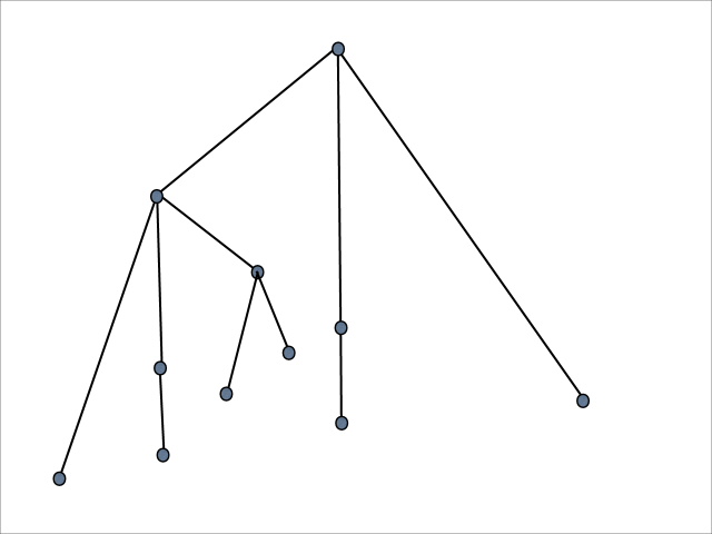
Figure 1: The cascade tree with the basal species (the vertex at the top) playing the role of the root. The height of this cascade tree is equal to 3.

We now turn to more subtle properties of the continuum cascade model which are related to the cascade tree. This tree is finite and it varies from realization to realization; accordingly, the properties of the cascade tree are probabilistic. To define these properties it is convenient to utilize a more traditional way of plotting trees; the cascade tree pictured above is presented on Fig. 1. This figure resembles binary search trees and both the relevant properties of binary search trees and the methods used in analysis of binary search trees [25, 26, 27, 28, 29, 30, 31, 32, 33, 34, 35, 36, 37] are useful in our situation. For instance, the height of the binary search trees has attracted a lot of attention, and a traveling wave analysis [33, 34, 35] has provided a very efficient way of tackling the asymptotic (in number of vertices of the tree) behavior of the height. In the present problem, the height is indeed an interesting quantity, namely it is the length of longest chain from the basal species to the bottom of the cascade tree, and the traveling wave analysis will be helpful as well.

We now establish a recurrence relation for the height distribution. The height is a non-negative integer. It is convenient to work with the cumulative distribution

$$P_{n}(x)={\rm Prob}({\rm height}\leq n)$$ (4)

The basal species is the terminal vertex with probability $e^{-x}$, and therefore

$$P_{0}(x)=e^{-x}$$ (5)

For $n\geq 1$,

$$P_{n}(x) = \sum_{k\geq 0}\frac{x^{k}}{k!}\,e^{-x}\int_{0}^{x}\cdots\int_{0}^{x}P_{n-1}(y_{1})\cdots P_{n-1}(y_{k})\,\frac{dy_{1}}{x}\cdots\frac{dy_{k}}{x}$$

$$= e^{-x}\sum_{k\geq 0}\frac{1}{k!}\left(\int_{0}^{x}P_{n-1}(y)\,dy\right)^{k},$$

where the first line accounts for any possible number $k\geq 0$ of links emanating from the origin and finishing at all possible points $x-y_{j}$. There is no ‘interaction’ between different branches of the cascade tree, so we merely must assure that all cascade trees originating at $x-y_{j}$ have heights not exceeding $n-1$. Computing the sum in the above equation we arrive at our main recurrence

$$P_{n}(x)=\exp\left[-x+\int_{0}^{x}P_{n-1}(y)\,dy)\right]$$ (6)

Starting with (5) we find

$$P_{1}(x)=\exp\!\left[-x+1-e^{-x}\right].$$ (7)

One can recursively determine $P_{2}$, then $P_{3}$; analytical expressions for $P_{n}$ become very cumbersome as $n$ increases. Fortunately, in the large ‘time’ limit, $n\gg 1$, the behavior greatly simplifies, namely the solution acquires a traveling wave form [see Fig. 2],

$$P_{n}(x)\to\Pi(\xi),\quad\xi=x-x_{f},$$ (8)

with the front position growing linearly with ‘velocity’ equal to $e^{-1}$:

$$x_{f}\simeq vn,\quad v=\frac{1}{e}$$ (9)

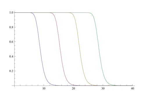
Figure 2: The distribution $P_{n}(x)$ versus $x$ obtained by iteration the recurrence (6). Shown is $P_{n}(x)$ for $n=20,40,60,80$ (left to right). Iterations were performed using Mathematica. The observed velocity of the traveling wave is in a good agreement with the theoretical prediction (9).

The traveling wave profile $\Pi(\xi)$ decreases monotonically from 1 to 0 as $\xi$ increases from $-\infty$ to $\infty$. More precisely,

$$\Pi(\xi)\propto e^{-\xi}\quad{\rm when}\quad\xi\to\infty$$ (10)

and

$$1-\Pi(\xi)\propto e^{e\xi}\quad{\rm when}\quad\xi\to-\infty$$ (11)

In the next section we give an elementary argument which allows one to understand (9). A more comprehensive traveling wave analysis that leads to above results is presented in section 4.

3 Elementary derivation of the traveling wave velocity

Let us begin with the behavior of $P_{n}(x)$ for small $x$. Expanding $P_{0}(x)$ and $P_{1}(x)$, see equation (7), we obtain

$$P_{0}=1-x+\frac{1}{2}x^{2}-\frac{1}{6}x^{3}+\ldots,\quad P_{1}=1-\frac{1}{2}x^{2}+\frac{1}{6}x^{3}+\frac{1}{12}x^{4}+\ldots$$

Using equation (6) we recurrently determine the expansions of the following $P_{n}$ to yield

$$P_{n}=1-\frac{1}{(n+1)!}x^{n+1}+\ldots$$ (12)

This result is easy to prove by induction. One can continue this expansion, e.g.,

$$P_{n}=1-\frac{1}{(n+1)!}x^{n+1}+\frac{1}{(n+2)!}x^{n+2}+\frac{2}{(n+3)!}x^{n+3}+\ldots$$ (13)

is valid for all $n\geq 1$; this is also easily proven by induction.

Let us now estimate the front position $x_{f}$ from the criterion $P_{n}(x_{f})=\frac{1}{2}$. Keeping only two terms as in equation (12) we obtain $x_{f}^{n+1}=\frac{1}{2}(n+1)!$, or $x_{f}=\frac{n+1}{e}$ in the leading order. What will happen if we keep e.g. four terms in the expansion? Using the same criterion $P_{n}(x_{f})=\frac{1}{2}$ in conjunction with equation (13) we get

$$\frac{x_{f}^{n+1}}{(n+1)!}\left[1-\frac{x_{f}}{n+2}-\frac{2x_{f}^{2}}{(n+2)(n+3)}\right]=\frac{1}{2}.$$

In the leading order we recover the previous prediction $x_{f}=\frac{n+1}{e}$. This does not prove equation (9), but at least it shows its consistency with the series (13).

4 Traveling wave analysis: Velocity selection

We want to understand the behavior of the recurrence

$$P_{n+1}(x)=\exp\!\left[-x+\int_{0}^{x}dy\,P_{n}(y)\right]$$ (14)

when $x\gg 1$. We assume the convergence to traveling wave solution and the validity of the traveling wave ansatz (8). Numerical results strongly support this assumption [see Fig. 2] and show that the convergence is rather fast, that is, the asymptotic shape emerges already for not to large $n$. We also assume that $x_{f}=vn$ (for large $n$), but we do not specify $v$. The left-hand side of equation (14) becomes

$$P_{n+1}(x)=\Pi(\xi-v)$$ (15)

while the right-hand side of equation (14) turns into

$$\exp\!\left[-x+\int_{-nv}^{\xi}d\eta\,\Pi(\eta)\right],\qquad\eta=y-nv$$ (16)

We will allow $|\xi|$ to be large, but we will always assume that $|\xi|\ll nv$. In this situation, the integral in equation (16) can be simplified as follows:

$$\int_{-nv}^{\xi}d\eta\,\Pi(\eta) = \int_{-nv}^{0}d\eta\,\Pi(\eta)+\int_{0}^{\xi}d\eta\,\Pi(\eta)$$ (17)

$$= nv+\int_{-nv}^{0}d\eta\,[\Pi(\eta)-1]+\int_{0}^{\xi}d\eta\,\Pi(\eta)$$

$$= nv+\int_{0}^{\xi}d\eta\,\Pi(\eta)-L+L_{n},$$

where we have used the shorthand notation

$$L=\int_{-\infty}^{0}d\eta\,[1-\Pi(\eta)],\quad L_{n}=\int_{-\infty}^{-nv}d\eta\,[1-\Pi(\eta)].$$ (18)

Since $\Pi(\eta)$ quickly approaches to 1 as $\eta\to-\infty$, we drop $L_{n}$ from (17); we shall justify this step a posteriori. Combining (16) and (17) we see that the right-hand side of (14) becomes

$$\exp\!\left[-\xi-L+\int_{0}^{\xi}d\eta\,\Pi(\eta)\right].$$ (19)

Equating (15) and (19) we arrive at

$$\Pi(\xi-v)=\exp\!\left[-\xi-L+\int_{0}^{\xi}d\eta\,\Pi(\eta)\right].$$ (20)

This is the governing equation for $\Pi(\xi)$.

4.1 Far ahead of the front: $\xi\to\infty$

Since $\Pi(\xi)$ quickly approaches to zero as $\xi\to\infty$, equation (20) gives $\Pi(\xi-v)\simeq e^{-\xi-L+R}$, where $R=\int_{0}^{\infty}d\eta\,\Pi(\eta)$. Thus we confirm (10); more precisely we get

$$\Pi(\xi)\simeq e^{R-L-v}\,e^{-\xi}\quad{\rm when}\quad\xi\to\infty.$$ (21)

4.2 Far behind the front: $\xi\to-\infty$

It is more convenient to work with $\Phi(\xi)=1-\Pi(\xi)$ rather than $\Pi(\xi)$. In terms of $\Phi(\xi)$, equation (20) becomes

$$1-\Phi(\xi-v)=\exp\!\left[-L-\int_{0}^{\xi}d\eta\,\Phi(\eta)\right].$$ (22)

From the definition (18) we see that

$$L=\int_{-\infty}^{0}d\eta\,\Phi(\eta).$$

Therefore we can re-write (22) as

$$1-\Phi(\xi-v)=\exp\!\left[-\int_{-\infty}^{\xi}d\eta\,\Phi(\eta)\right].$$ (23)

Equation (23) is equivalent to Eq. (20), we have not made any approximation. Turning to the $\xi\to-\infty$ limit we note that in this regime $\Phi\to 0$ and hence we can expand the exponent on the right-hand side of equation (23). Keeping only two terms we simplify equation (23) to

$$\Phi(\xi-v)=\int_{-\infty}^{\xi}d\eta\,\Phi(\eta).$$ (24)

From (24), or from equation $\Phi^{\prime}(\xi-v)=\Phi(\xi)$ obtained by differentiating of Eq. (24), we see that the solution has an exponential form

$$\Phi(\xi)=D\,e^{a\xi}$$ (25)

Plugging (25) into (24) we arrive at the dispersion relation

$$a\,e^{-av}=1$$ (26)

An elementary analysis of this equation indicates that solutions exist only when $v\leq e^{-1}$. We now invoke the selection principle which asserts that the extremal value, $v=e^{-1}$ in our case, is realized.

Traveling wave solutions have been investigated in the context of partial differential equations. A few partial differential equations admitting traveling wave solutions have been deeply studied. One such equation is the celebrated Fisher-KPP equation [38, 39] for which the selection principle had been proven [39, 40] for sufficiently steep initial conditions. (For more recent work see e.g. [41, 42, 43]. A very comprehensive review of traveling wave solutions of non-linear partial differential equations has been given by van Saarloos [44], a lighter expositions appear in books [45, 46, 9].) More recently, traveling wave solutions have been investigated in the context of nonlinear recurrences arising in the analyses of binary search algorithms [33, 34, 35], kinetic theory [47], and other problems [48, 49, 50, 51]; see [52, 53] for a review of the applications of traveling wave techniques to recurrences.

Asymptotically, the wave front advances at a constant velocity $v=e^{-1}$. The approach to this asymptotic value is rather slow, namely there is a $n^{-1}$ correction in the leading order, resulting in a logarithmic correction to the front position. This correction was first established by Bramson [40] for the Fisher-KPP equation; it was subsequently generalized [41, 42, 43, 44] to more general partial differential equations and to recurrences [33, 34, 35, 48, 49]. This correction generally has the form $\frac{3}{2a}\ln n$. For the selected velocity $v=e^{-1}$, the decay amplitude $a=e$ is implied by dispersion relation (26). Taking into account this logarithmic correction we get

$$x_{f}=e^{-1}n+\frac{3}{2e}\,\ln n+\mathcal{O}(1)$$ (27)

It was convenient to think about $x$ and $n$ as space and time coordinates, so that the front of the traveling wave was advancing and we determined $x_{f}=x_{f}(n)$. In the original problem, the parameter $x$ is fixed and we are interested in the height $H(x)$ of the cascade tree. The height is essentially the inverse to $x_{f}=x_{f}(n)$ which is taken when $x_{f}=x$. Thus

$$H(x)=ex-\frac{3}{2}\,\ln x+\mathcal{O}(1)$$ (28)

The height is of course a random quantity. Equation (28) gives the average height. In the $x\to\infty$ limit, the average provides a faithful description as it is a growing quantity while the variance remains finite. We haven’t proved this assertion, but at least on the physical level of rigor it is obvious: The probability distribution $Pn(x)$ has asymptotically a traveling wave shape with the width of the front remaining finite, and this is essentially equivalent to the finite width of the height distribution.

5 Size of the Cascade Tree

The size $S(x)$ of the cascade tree, that is, the total number of vertices in the tree, is a random variable. Let us compute the average size $\langle S(x)\rangle$. From the definition of the continuum cascade model we deduce

$$\langle S(x)\rangle = 1+\sum_{k=1}^{\infty}\frac{x^{k}}{k!}\,e^{-x}\int_{0}^{x}\cdots\int_{0}^{x}\frac{dy_{1}}{x}\cdots\frac{dy_{k}}{x}\left[\langle S(y_{1})\rangle+\cdots+\langle S(y_{k})\rangle\right]$$ (29)

$$= 1+\sum_{k=1}^{\infty}\frac{x^{k}}{k!}\,e^{-x}k\int_{0}^{x}\frac{dy}{x}\,\langle S(y)\rangle$$

$$= 1+\int_{0}^{x}dy\,\langle S(y)\rangle$$

Differentiating (29) we obtain $\frac{d\langle S\rangle}{dx}=\langle S\rangle$, from which

$$\langle S(x)\rangle=e^{x}$$ (30)

A similar line of reasoning leads to an integral equation for the second moment

$$\langle S^{2}(x)\rangle = 1+\sum_{k=1}^{\infty}\frac{x^{k}}{k!}\,e^{-x}k\int_{0}^{x}\frac{dy}{x}\,\langle S^{2}(y)\rangle+2\sum_{k=1}^{\infty}\frac{x^{k}}{k!}\,e^{-x}k\int_{0}^{x}\frac{dy}{x}\,\langle S(y)\rangle$$

$$+ \sum_{k=1}^{\infty}\frac{x^{k}}{k!}\,e^{-x}\,\frac{k(k-1)}{2}\int_{0}^{x}\frac{dy_{1}}{x}\,\langle S(y_{1})\rangle\int_{0}^{x}\frac{dy_{2}}{x}\,\langle S(y_{2})\rangle$$

Using (30) we simplify above integral equation to

$$\langle S^{2}(x)\rangle=1+\int_{0}^{x}dy\,\langle S(y)\rangle+2(e^{x}-1)+(e^{x}-1)^{2}$$

which is solved to yield

$$\langle S^{2}(x)\rangle=2e^{2x}-e^{x}$$ (31)

One can continue and compute

$$\langle S^{3}(x)\rangle=\frac{15}{4}\,e^{3x}-\frac{11}{4}\,e^{x}-\frac{3}{2}\,xe^{x}$$ (32)

and a few higher moments $\langle S^{p}(x)\rangle$, but results quickly become very cumbersome. The explicit results (30)–(32) show that, in contrast to the height, the size of the cascade tree is the random quantity whose limiting distribution (in the $x\to\infty$ limit) remains broad. More precisely, in the scaling limit

$$x\to\infty,\quad S\to\infty,\quad\sigma=e^{-x}S={\rm finite}$$

the size distribution becomes

$${\rm Prob}[S(x)=S]=e^{-x}F(\sigma)$$

with the limiting distribution being different from the delta function, $F(\sigma)\neq\delta(\sigma-1)$. The normalization requirement together with (30)–(32) and similar equations for higher moments $\langle S^{p}(x)\rangle$ show that the moments $M_{p}=\int_{0}^{\infty}d\sigma\,\sigma^{p}F(\sigma)$ of the limiting distribution are

$$M_{0}=M_{1}=1,\quad M_{2}=2,\quad M_{3}=\frac{15}{4}\,,\quad M_{4}=\frac{34}{3}\,,\quad M_{5}=25,$$

etc.

6 Summary

We proposed a minimalist model of infinite directed random graphs. The model is a continuum version of a model of finite directed random graphs, known as the cascade model, which has been investigated in the context of food webs and parallel computation.

Our model presumes a total order on the set of vertices. We chose the simplest such set, an interval of length $x$. From each $y\in[0,x]$, directed links to points $y^{\prime}>y$ are drawn at random according to the Poisson distribution, that is, the points $y^{\prime}\in(y,x]$ are chosen independently from each other and uniformly with density one. The analysis of this continuum cascade model is actually simpler than the analysis of the discrete cascade model. This is demonstrated by studying the distribution of the length of the longest directed paths starting at the origin (equivalently, the height of the cascade tree with the root at the origin). We employed traveling wave techniques to extract the asymptotic behavior of the length of the longest directed paths in the $x\to\infty$ limit. It will be interesting to understand the limiting distribution of the size of the cascade tree with the root at the origin as well as other properties of the continuum cascade model.

Acknowledgment YI thanks Joel E. Cohen for helpful comments and discussions. YI is supported in part by US National Science Foundation Grant DMS 0443803 to Rockefeller University and by JSPS Grant-in-aid for Scientific Research 23540177.

References

References

- [1] Solomonoff R and Rapaport A 1959 Connectivity of random nets Bull. Math. Biophys. 13 107–117
- [2] Erdős P and Rényi A 1960 On the evolution of random graphs Publ. Math. Inst. Hungar. Acad. Sci. 5 17–61
- [3] Bollobás B 1985 Random Graphs (London: Academic Press)
- [4] Shepp L A 1989 Connectedness of certain random graphs Israel J. Math. 67 23–33
- [5] Durrett R and Kesten H 1990 The critical parameter of the connectedness of some random graphs, A Tribute to Paul Erdős, 161–176 (Cambridge: Cambridge University Press)
- [6] Janson S, Knuth D E, Łuczak T and Pittel B 1993 The birth of the giant component Rand. Struct. Alg. 3 233–358
- [7] Janson S, Luczak T and Rucinski A 2000 Random Graphs (New York: John Wiley & Sons)
- [8] Flory P F 1953 Principles of Polymer Chemistry (Ithaca: Cornell University Press)
- [9] Krapivsky P L, Redner S and Ben-Naim E 2010 A Kinetic View of Statistical Physics (Cambridge: Cambridge University Press)
- [10] Newman M E J 2002 Spread of epidemic disease on networks Phys. Rev. E 66 016128
- [11] Caldarelli G 2007 Scale-Free Networks: Complex Webs in Nature and Technology (Oxford: Oxford University Press)
- [12] Dorogovtsev S N and Mendes J F F 2003 Evolution of Networks: From Biological Nets to the Internet and WWW (Oxford: Oxford University Press)
- [13] Newman M E J 2010 Networks: An Introduction (Oxford: Oxford University Press)
- [14] Broder A, Kumar R, Maghoul F, Raghavan P, Rajagopalan S, Stata R, Tomkins A and Wiener J 2000 Graph structure in the web Computer Networks 33 309–320
- [15] Krapivsky P L, Rodgers G J and Redner S 2001 Degree distributions of growing networks Phys. Rev. Lett. 86 5401–5404
- [16] Krapivsky P L and Redner S 2002 A statistical physics perspective on web growth Computer Networks 39 261–276
- [17] Cohen J E 1990 A stochastic theory of community food webs VI. Heterogeneous alternatives to the cascade model Theor. Popul. Biol. 37 55–90
- [18] Cohen J E, Briand F and Newman C M 1990 Community food webs: Data and Theory (New York: Springer-Verlag)
- [19] Cohen J E and Newman C M 1985 A stochastic theory of community food webs: I. Models and aggregated data Proc. R. Soc. (London) B 224 421–448
- [20] Cohen J E, Briand F and Newman C M 1986 A stochastic theory of community food webs III. Predicted and observed lengths of food chains Proc. R. Soc. (London) B 228 317–353
- [21] Cohen J E and Newman C M 1986 A stochastic theory of community food webs IV. Theory of food chain length in large webs Proc. R. Soc. (London) B 228 355–377
- [22] Newman C M 1992 Chain lengths in certain random directed graphs Rand. Struct. Alg. 3 243–253
- [23] Gelenbe E, Nelson R, Philips T and Tantawi A 1986 An approximation of the processing time for a random graph model of parallel computation, ACM 86 Proceedings of 1986 ACM Fall joint computer conference IEEE Computer Society Press, Los Alamos, 691–697
- [24] Isopi M and Newman C M 1992 Speed of parallel-processing for random task graphs Commun. Pure Appl. Math. 47 361–376
- [25] Drmota M 2009 Random Trees: An Interplay between Combinatorics and Probability (Wien: Springer)
- [26] Sibuya M and Itoh Y 1987 Random sequential bisection and its associated binary tree Ann. Inst. Stat. Math. 39 69–84
- [27] Hattori T and Ochiai H 2006 Scaling limit of successive approximations for Funkcialaj Ekvacioj 39 291–319
- [28] Janson S and Neininger R 2008 The size of random fragmentation trees Probab. Theory Rel. Fields 142 399–442
- [29] Dutour Sikiric M and Itoh Y 2011 Random Sequential Packing of Cubes (London: World Scientific)
- [30] Robson J M 1979 The height of binary search trees, Australian Comput. J. 11 151–153
- [31] Flajolet P and Odlyzko A 1982 The average height of binary tree and other simple tree J. Comput. Syst. Sci. 25 171–213
- [32] Devroye L 1986 A note on the height of binary search trees J. ACM 33 489–498
- [33] Krapivsky P L and Majumdar S N 2000 Traveling waves, front selection, and exact nontrivial exponents in a random fragmentation problem Phys. Rev. Lett. 85 5492–5495
- [34] Ben-Naim E, Krapivsky P L and Majumdar S N 2001 Extremal properties of random trees Phys. Rev. E 64 035101
- [35] Majumdar S N and Krapivsky P L 2002 Extreme value statistics and traveling fronts: Application to computer science Phys. Rev. E 65 036127
- [36] Szpankowski W 2001 Average case analysis of algorithms on sequences (New York: Wiley)
- [37] Itoh Y 2011 Random sequential generation of intervals for the cascade model of food webs arXiv:1106.4701
- [38] Fisher R A 1937 The wave of advance of advantageous genes Ann. Eugenics 7 355–369
- [39] Kolmogorov A, Petrovsky I, and Piskunov N 1937 Mosc. Univ. Bull. Math. A 1 1; translated and reprinted in P. Pelce 1988 Dynamics of Curved Fronts (San Diego: Academic)
- [40] Bramson M 1983 Convergence of Solutions of the Kolmogorov Equation to Traveling Waves American Mathematical Society, Providence, R.I.
- [41] Brunet E and Derrida B 1997 Shift in the velocity of a front due to a cut-off Phys. Rev. E 56 2597–2604.
- [42] Ebert U and van Saarloos W 1998 Universal algebraic relaxation of fronts propagating into an unstable state and implications for moving boundary approximations Phys. Rev. Lett. 80 1650–1653
- [43] Ebert U and van Saarloos W 2000 Front propagation into unstable states: universal algebraic convergence towards uniformly translating pulled fronts Physica D 146 1–99
- [44] van Saarloos W 2003 Front propagation into unstable states Phys. Rep. 386 29–222
- [45] Murray J D 1989 Mathematical Biology (New York: Springer-Verlag)
- [46] Barenblatt G I 1995 Scaling, Self-Similarity, and Intermediate Asymptotics (Cambridge: Cambridge University Press)
- [47] van Zon R, van Beijeren H and Dellago Ch 1998 Largest Lyapunov exponent for many particle systems at low densities Phys. Rev. Lett. 80 2035
- [48] Majumdar S N and Krapivsky P L 2000 Extremal paths on a random Cayley tree Phys. Rev. E 62 7735–7742
- [49] Majumdar S N and Krapivsky P L 2001 The dynamics of efficiency: A simple model Phys. Rev. E 63 045101(R)
- [50] Majumdar S N Traveling front solutions to directed diffusion limited aggregation, digital search trees and the Lempel-Ziv data compression algorithm Phys. Rev. E 68 026103
- [51] D’Souza R M, Krapivsky P L and Moore C 2007 The power of choice in growing trees Eur. Phys. J. B 59 535–543
- [52] Majumdar S N and Krapivsky P L 2003 Extreme value statistics and traveling fronts: Various applications Physica A 318, 161–170
- [53] Majumdar S N, Dean D S and Krapivsky P L 2005 Understanding search trees via statistical physics Pramana J. Phys. 64, 1175–1189