Antibound poles in cutoff Woods–Saxon and in Salamon–Vertse potentials

Abstract

The motion of $l=0$ antibound poles of the $S$-matrix with varying potential strength is calculated in a cutoff Woods–Saxon (WS) potential and in the Salamon–Vertse (SV) potential, which goes to zero smoothly at a finite distance. The pole position of the antibound states as well as of the resonances depend on the cutoff radius, especially for higher node numbers. The starting points (at potential zero) of the pole trajectories correlate well with the range of the potential. The normalized antibound radial wave functions on the imaginary $k$-axis below and above the coalescence point have been found to be real and imaginary, respectively.

I Introduction

Nuclear states are most often described in terms of single-particle (s.p.) bases generated by a spherical potential, mostly of Woods–Saxon (WS) type. Bound and discrete unbound s.p. states all obey the outgoing-wave boundary condition, which is $u(r,k)\sim\exp(ikr)$ when both the charge and the angular momentum $l$ are 0. The general solution behaves like $\exp(-ikr)-S\exp(ikr)$, where $S$, a function of the energy $E$ or the wave number $k$, is called the S-“matrix”. Where the outgoing boundary condition is satisfied, the S-matrix has poles. The bound-state poles belong to $E<0$ or imaginary wave number with ${\rm Im}\,k\equiv\gamma>0$. The resonance poles belong to complex $E$ and $k$, with $k=\pm\kappa-{\rm i}\gamma$ ($\kappa,\,\gamma>0$). For antibound (virtual) states, $E<0$, $k=-{\rm i}\gamma$ ($\gamma>0$).

A WS basis is only complete if, in addition to bound states, it contains continuum scattering states and/or resonances and/or antibound states [Be68] ; [Mi09] . The completeness is understood with respect to a generalized scalar product. The resonance states, which have definite intuitive meanings, have proved to be very useful in describing weakly bound or unbound states of nuclei [Mi09] , unlike antibound states, whose exponential tail, $\exp(\gamma r)$, looks unphysical. However, the inclusion of an antibound state of ¹⁰Li [Ma00] in the description of ^11,12Li was found meaningful [Lov04] ; [Bet04] ; [Bet05] ; [Xu11] . This shows that antibound states and the corresponding S-matrix poles (“antibound poles”) do deserve some attention.

As an extension of recent studies [Sa08] ; [ra11] of the dependence of the S-matrix poles on the tail behavior of the potential, we now study antibound poles. The nuclear potential should in principle have an exponentially decreasing tail, like the folding of the nuclear matter density with the one-pion exchange force. The standard WS potential obeys this criterion, but it can only be treated properly in analytical calculations, and analytical solution to the Schrödinger equation with a WS potential [Ben66] only exists for angular momentum zero. The matter is that in numerically solving the problem with a prescribed boundary condition the solution has to be matched, at a finite distance, to the solution with potential zero (asymptotic solution), and the matching amounts to cutting off the tail of the potential. The error committed in this way is usually believed to be small, but in a recent paper it was shown that, for broad resonances, the poles in a cutoff WS potential strongly depend on the value of the cutoff radius [Sa08] ; [ra11] .

In this work we examine the effect of the cutoff on the WS potential, and compare its behavior with a potential that goes to zero smoothly and is exactly zero beyond a point. This “Salamon–Vertse (SV) potential” contains as many parameters as a cutoff WS potential and its shape is similar except for its tail. The tail of the SV potential can only conform to that of the WS at the expense of the inner region. Conformity in a longer section can be achieved with more parameters. This paper is only concerned with pointing out where problems might appear because of the cutoff.

Unlike in former studies of antibound states we are aware of [Nu59] ; [Mi09] , we now explore the wave functions as well. We limit our attention to $l=0$ since antibound states may only play some role for s-states.

II Potentials

In solving the radial Schrödinger equation, a numerically calculated inner solution has to be matched at a distance $r=r_{a}$ to the solution of the asymptotic equation, and that yields the $S$-matrix. This procedure is tantamount to cutting off the WS potential at $r=R_{\rm max}\leq r_{a}$. The potentials will be given in a form that expresses that they are exactly zero beyond a point, i.e., they are of finite range in a strict sense. The cutoff WS potential is thus

$$V^{\rm WS}(r)=V_{0}f^{\rm WS}(r),$$ (1)

with

$$f^{\rm WS}(r)=\left\{\begin{array}[]{rl}-\left(1+{\rm e}^{\frac{r-R}{a}}\right)^{-1}&\textrm{, if }r<R_{\rm max}\\ 0{}{}{}{}&\textrm{, if }r\geq R_{\rm max}.\end{array}\right.$$ (2)

In the resonance region the pole trajectories obtained by varying $V_{0}$ do depend on the cutoff radius $R_{\rm max}$ [ra11] .

The SV potential becomes zero beyond a finite value $r\geq\rho_{0}$ such that all its derivatives are also zero. Thus the potential is differentiable in the whole domain $r\in[0,\infty)$, in contrast with the cutoff WS potential, which has a discontinuity at the cut.

To follow Eq. (1), we write the SV potential as

$$V^{SV}(r)=V_{0}f^{SV}(r),$$ (3)

where

$$f^{SV}(r)\equiv f^{SV}(r,c_{1},\rho_{0},\rho_{1})=f_{\rho_{0}}(r)-c_{1}f^{\prime}_{\rho_{1}}(r),$$ (4)

with

$$f_{\rho}(r) = \left\{\begin{array}[]{rl}-{\rm e}^{\frac{r^{2}}{r^{2}-\rho^{2}}}&\textrm{, if }r<\rho\\ 0{}{}{}{}&\textrm{, if }r\geq\rho,\end{array}\right.$$ (7)

$$f^{\prime}_{\rho}(r) = \left\{\begin{array}[]{rl}{\frac{2r\rho^{2}}{(r^{2}-\rho^{2})^{2}}}{\rm e}^{\frac{r^{2}}{r^{2}-\rho^{2}}}&\textrm{, if }r<\rho\\ 0{}{}{}{}{}{}{}{}&\textrm{, if }r\geq\rho.\end{array}\right.$$ (10)

The range parameters $\rho_{0}$ and $\rho_{1}$ are chosen as $\rho_{0}>\rho_{1}$, thus the potential in Eq. (3) vanishes at $\rho_{0}$. To make the SV potential conform to the WS potential, we fit its three parameters, $\rho_{0}$, $\rho_{1}$ and $c_{1}$ ($c_{1}>0)$, to the WS form $f^{\rm WS}(r)$ [ra11] .

To have several antibound poles in the same potential, we choose the neutron potential to represent a heavy nucleus, ²⁰⁸Pb. The values $R=1.27\times 208^{1/3}$ fm $=7.525$ fm, $a=0.7$ fm were adopted [Cu89] , with $R_{\rm max}=15$ fm. The SV parameters giving the best fit to the WS shape are: $c_{1}=0.997$, $\rho_{0}=10.963$ fm and $\rho_{1}=8.328$ fm [ra11] .

III Wave functions

Let us sketch briefly how the pole solutions of the radial equation are calculated. For $l=0$ the radial equation is

$$\frac{d^{2}u(r,k)}{dr^{2}}+[k^{2}-U(r)]u(r,k)=0\,,$$ (11)

where $U(r)=(2\mu/\hbar^{2})V(r)$. We introduce an intermediate distance $R_{\rm im}$, where the internal (“left”) and external (“right”) solutions are to be matched. The left solution is defined in the interval $r\in[0,R_{\rm im}]$ such that

$$u_{\rm left}(0,k)=0,\quad\quad\left.\frac{du_{\rm left}(r,k)}{dr}\right|_{r=0}\equiv u^{\prime}(0,k)=1.$$ (12)

The right solution is defined in the interval $r\in[R_{\rm im},r_{\rm a}]$, where $r_{\rm a}$ is in the asymptotic region ($r_{\rm a}\geq R_{\rm max}$ and $r_{\rm a}\geq\rho_{0}$), so that the solution satisfy the boundary condition

$$u_{\rm right}(r_{\rm a},k)={\rm e}^{ikr_{\rm a}}\quad\left(u^{\prime}_{\rm right}(r_{\rm a},k)=ike^{ikr_{\rm a}}\right).$$ (13)

We integrate Eq. (11) numerically starting from the origin up to $R_{\rm im}$ and from $r_{\rm a}$ down to $R_{\rm im}$. The eigenvalue or pole position is defined as the $k$ value for which the left and right logarithmic derivatives

$$L_{\rm left}(k)=\frac{u_{\rm left}^{\prime}(R_{\rm im},k)}{u_{\rm left}(R_{\rm im},k)},\,\,\,L_{\rm right}(k)=\frac{u_{\rm right}^{\prime}(R_{\rm im},k)}{u_{\rm right}(R_{\rm im},k)}$$ (14)

are equal:

$$L_{\rm left}(k_{j})-L_{\rm right}(k_{j})=0,$$ (15)

where, for antibound states, $k_{j}=-i\gamma_{j}$ ($\gamma_{j}>0$), with $j$ denoting the sequence number of the state. If we introduce the matching factor $a_{\rm left}=u_{\rm right}(R_{\rm im},k_{j})/u_{\rm left}(R_{\rm im},k_{j})$ of the left solution, the eigensolution

$$v(r,k_{j})=\left\{\begin{array}[]{rl}a_{\rm left}u_{\rm left}(r,k_{j})&\textrm{, if }r<R_{\rm im}\\ u_{\rm right}(r,k_{j})&\textrm{, if }r\geq R_{\rm im}\end{array}\right.$$ (16)

obtained in this way is well matched but not normalized.

Since $\int_{r_{\rm a}}^{\infty}\exp(2ikr)dr=\infty$ for $k=-i\gamma$ with $\gamma>0$, the norm of an antibound state is infinity in the normal sense. By truncating the norm integral $\int_{0}^{\infty}v^{2}(r,k_{j})dr$ at $r=r_{\rm a}$, the result will depend on $r_{\rm a}$ through a term $(2ik_{j})^{-1}\exp(2ik_{j}r_{\rm a})$, which has to be eliminated. For resonance states this term can be eliminated either by using the prescription of Hokkyo [Ho65] , or by rotating the integration path of $\int_{r_{\rm a}}^{\infty}\exp(2ikr)dr$ onto the complex $r$-plane to the extent that the primitive function go to zero in infinity [GyV71] , which results in $-(2ik)^{-1}\exp(2ikr_{\rm a})$ for the integral, and cancels the spurious dependence on $r_{\rm a}$ resulting from $\int_{0}^{r_{\rm a}}v^{2}(r,k_{j})dr$. This rotation of the integration path provides a sound generalization for the scalar product involving Gamow resonances [Be68] , and makes it possible to construct complete sets involving resonance states. The same prescription also sets the tail term of the norm integral of an antibound state to $-(2ik)^{-1}\exp(2ikr_{\rm a})$ if a more radical rotation (by an angle $>\pi$) is applied, and the results with this formula are meaningful [Ve87] . It is this prescription that allows the inclusion of antibound states in complete sets of states [Ve89] .

With this, the square of the norm of $v(r,k_{j})$ is

$$N^{2}=\int_{0}^{r_{a}}v^{2}(r,k_{j})dr-C(r_{a},k_{j}),$$ (17)

where

$$C(r,k)=\frac{e^{2ikr}}{2ik}.$$ (18)

The antibound wave function normalized to $1$ is thus

$$u(r,k_{j})=\frac{1}{N}v(r,k_{j}).$$ (19)

For $k_{j}=-i\gamma_{j}$ ($\gamma_{j}>0$), the term $C(r_{a},k_{j})$ is positive, just as the first term in Eq. (17). Thus $N^{2}$ may be either positive or negative, a fortiori $N$ as well as $u(r,k_{j})$ may be real or imaginary. Since the radial wave function $u$ enters in the norm integral as $u^{2}$, and $u$ must not be complex conjugated in any matrix elements [Be68] , the imaginary wave function causes a strange behavior [Lov04] .

The pole positions $k_{j}$ and the corresponding normalized radial wave functions were calculated by a modified version of the computer code GAMOW [Ve82] . The accuracy of the calculation was checked by a more accurate program ANTI [Ix95] using Ixaru’s CP method [Ix84] .

IV Numerical results

IV.1 Qualitative behavior of antibound poles

Figures 2 and 2 show the imaginary part of the pole wave number $k$ as a function of the potential depth for the WS and for the SV potential, respectively. For bound and antibound states ${\rm Re}\,(k)=0$. For a very shallow potential, there is just one antibound state, with node number $n=0$. With the attraction increased, the pole passes through the origin at $V_{0}=V_{0,0}$, and the system becomes bound. The ${\rm Im}\,(k)$ versus $V_{0}$ curves belonging to the other poles look like parabolas with horizontal axes. The bound states become antibound as the potential depth is decreased to $V_{0,n}$, and meet another antibound pole at $V_{n}$. What happens beyond their coalescence can only be depicted on the complex $k$-plane (Fig. 3). The two poles part the ${\rm Im}\,(k)$-axis perpendicularly in opposite directions [Ne82] .

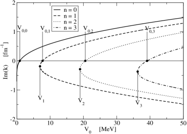
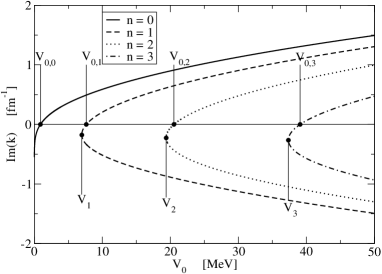
Figure 1: Imaginary part of the pole wave number as a function of the depth of the WS potential. For bound and unbound states ${\rm Im}\,(k)>0$ and ${\rm Im}\,(k)<0$, respectively.

Figure 2: Imaginary part of the pole wave number as a function of the depth of the SV potential.

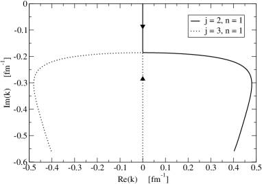
Figure 3: Trajectories of the two $n=1$, $l=0$ poles in the WS potential with $V_{0}$ varied ($R_{\rm max}=15$ fm).

We thus see that, while the bound state poles all move upwards along the imaginary $k$-axis when the potential is deepened, some antibound states behave conversely. The energy shift caused by a perturbation $\delta V_{0}f(r)$ can be estimated by $\delta E=\int_{0}^{r_{\rm a}}u^{2}(r,k_{j})\delta V_{0}f(r)dr$. The sign of $\delta E$ with respect to that of $\delta V_{0}f(r)$ depends on whether $u(r,k_{j})$ is real or imaginary. By looking at the $V_{0}$ dependence of the pole, we can unambiguously infer that the wave function is imaginary on the upper branches of the parabolas, and they are real below. The single $n=0$ antibound-state wave function is imaginary.

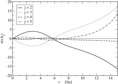
Figure 4: Normalized radial wave functions of antibound states in WS potentials. The $n=1$ ($j=2,3$) and $n=2$ ($j=4,5$) states were produced by $V_{0}=6.9692$ and 19.5 MeV, respectively. The wave numbers $k_{j}$ (in fm^-1) are $k_{2}=-0.183\,{\rm i}$, $k_{3}=-0.188\,{\rm i}$, $k_{4}=-0.410\,{\rm i}$, $k_{5}=-0.422\,{\rm i}$. The functions with $j=2,4$ are imaginary, while those with $j=3,5$ are real.

In Fig. 4 we show the radial wave functions of some normalized antibound states in WS potentials. The antibound states that belong to the same node number in two different branches of the parabola seem to be non-orthogonal to each other although they are generated, pairwise, by the same potential. That is, however, just an appearance. In fact, the tail region of the overlap integral cancels the the contribution of the inner region. The $j=2$ and $j=3$ antibound states are orthogonal to each other, and so are the $j=4$ and $j=5$ states. Thus, pairwise, they may be included in complete sets of states [Be68] simultaneously. (The antibound states of different node numbers are, of course, orthogonal to each other if, unlike in Fig. 4, they are produced by the same potential.)

If we have a centrifugal or Coulomb barrier, the picture is different in that the bound-state poles meet the antibound poles at the origin, and bifurcate there into a pair of resonance poles. In the ($V_{0}$,${\rm Im}\,(k)$) plane this corresponds to parabolas whose apices are at the origin. When the potential bottom is lifted, the antibound poles approach the origin monotonously from below, thus their normalized wave function is real throughout.

IV.2 Quantitative observations

A numerically most sensitive quantity is the apex $V_{n}$ of the parabolas in Fig. 2, and that was used for testing the $R_{\rm max}$-dependence for the WS potential (Table 1). We see that for $n=1,2,3$ the $V_{n}$ values are practically independent of $R_{\rm max}$. The largest variation is in $V_{3}$, most probably due to the enhancement of the error in the numerical solution of the differential equation as discussed in Ref. [Bo95] . The $k$-values of the apices are somewhat more sensitive to $R_{\rm max}$, and the sensitivity gets more pronounced for higher $n$. (We will return to this problem in discussing $R_{\rm max}$-dependence of the pole trajectories, see Fig. 7 later.) The sensitivity to the potential shape has also been tested by comparing the values obtained for the potential strength $V_{0,n}$, which puts the pole at the threshold (Table 2). For WS, $R_{\rm max}=15$ fm was used, but it was ascertained that $V_{0,n}$ is practically independent of $R_{\rm max}\in[15,25]$ fm. The strengths for the two potential forms are very similar, which follows from the shapes being very similar.

Table 1: Well depths $V_{n}$ at the coalescence of the two antibound poles

	$R_{\rm max}$ (fm)	$V_{1}$ (MeV)	$V_{2}$ (MeV)	$V_{3}$ (MeV)
WS	15	6.969	18.995	36.286
	16	6.969	18.992	36.263
	18	6.968	18.989	36.239
	20	6.968	18.989	36.239
	25	6.968	18.989	36.230
SV		6.978	19.378	37.347

Table 2: The values $V_{0,n}$ setting the pole at the threshold

Potential	$V_{0,0}$ (MeV)	$V_{0,1}$ (MeV)	$V_{0,2}$ (MeV)	$V_{0,3}$ (MeV)
WS	0.897	7.727	20.562	39.122
SV	0.893	7.634	20.519	39.072

As we showed in Fig. 3, beyond the coalescence, the pair of antibound poles is transformed into a pair of decaying and capturing resonance poles. We show the trajectories of some of the $l=0$ decaying resonances in the complex $k$-plane in Fig. 5. (The poles of the capturing resonances are the mirror images of the decaying ones with respect to the ${\rm Im}\,(k)$-axis.)

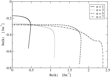
Figure 5: Trajectories of the odd-$n$, $l=0$ poles in the SV potential with $V_{0}$ varied. The even-$n$ trajectories are similar, except for $n=0$, which runs along the imaginary $k$-axis.

The starting point of a trajectory is defined by the limit $k_{j}=\lim_{V_{0}\to 0}\,{k_{j}(V_{0})}$. For a potential of range $R$, an estimate for this limit is given by [Ne82]

$${\rm Re}\,(k_{n})=\frac{n\pi}{R}+O(1).$$ (20)

For large $n$ we can perhaps neglect the term $O(1)$. We approximate $V_{0}=0$ by 5 keV.

In Fig. 5 one can see the trajectories of the $l=0$, $n=1,3,5,7$ poles in the SV potential. Only the (anti)bound states have definite node numbers $n$, but resonances can also be characterized by the node number of the (anti)bound state that they correspond to. The real parts of the starting points are seen to be almost equidistant. Therefore, these ${\rm Re}\,(k_{n})$ values can be fitted well by the straight line: ${\rm Re}\,(k_{n})=a_{0}+a_{1}n$, with a slope $a_{1}=0.32$ fm^-1, which implies $R=9.778$ fm.

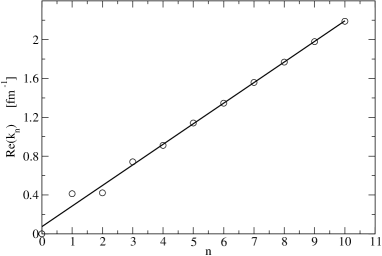
Figure 6: ${\rm Re}\,(k_{n})$ values of starting points of resonance trajectories for the WS potential cut off at $R_{\rm max}=15$ fm fitted with a straight line

As for the WS potential, in Fig. 6 one can see the starting points ${\rm Re}\,(k_{n})$ as a function of $n$, and a straight line fitted to it. Although, for $n<4$, the ${\rm Re}\,(k_{n})$ values are somewhat erratic, the slope of the line, $a_{1}=0.212$ fm^-1, provides $R=14.82$ fm, in good agreement with $R_{\rm max}=15$ fm. To see the dependence of the $R$ value deduced in this manner on $R_{\rm max}$, we repeated the calculations for a set of $R_{\rm max}$ values chosen from the range typically used in practical calculations. The slope of the line was determined from five points with $n=4,\ldots,8$. The results are given in Table 3. The smaller $R_{\rm max}$, the better is the agreement with $R$, and the better is Eq. (20) satisfied. For larger $R_{\rm max}$ the rund-off errors of the numerical solution of the radial equation get larger. This fact forbids one to go substantially beyond $R_{\rm max}=20$ fm.

Table 3: Ranges $R$ obtained from Eq. (20) for different values of the cutoff radii $R_{\rm max}$. The trajectory starting points ${\rm Re}\,(k_{n})$ were fitted by a linear function of $n$, and $R$ was calculated from its slope. The $\sigma$ values show the quality of the fit of the data to the straigt line.

$R_{\rm max}$ (fm)		$R$ (fm)		$\sigma$
11		10.93		$1.6\times 10^{-6}$
14		13.85		$2.0\times 10^{-5}$
17		16.89		$2.0\times 10^{-5}$
20		20.45		$6.4\times 10^{-4}$

We examined the sensitivity of the pole trajectories to the cutoff radius, and in Fig. 7 we illustrate the results with the case of $n=7$, which, for $R_{\rm max}=15$ fm, fits well into the straight line in Fig. 6. In view of the approximate independence of $V_{n}$ on $R_{\rm max}$ (see Table 1), the results look surprising. We see that the $n=7$ trajectory and, indeed, its point of intersection with the imaginary $k$-axis, depend appreciably on the cutoff. While $R_{\rm max}$ is changed between 11 fm and 20 fm, the intersection of the trajectories with the Im$\,(k)$-axis moves from $-{\rm i}0.40$ fm^-1 to $-{\rm i}0.61$ fm^-1, with the potential depth to be set to 166 and 159 MeV, respectively. Thus, similarly to the $n=1,\,2,\,3$ cases, $V_{7}$ is less sensitive to $R_{\rm max}$ than the pole positions.

The stability of $V_{n}$ as a function of $R_{\rm max}$ can be understood, again, in a perturbative picture. The shift of a pole energy caused by changing the cutoff radius $R_{\rm max}$ from $R_{1}$ to $R_{2}$ can be estimated to be $\Delta E=\int_{R_{1}}^{R_{2}}V^{\rm WS}(r)u^{2}(k_{j},r)dr$. Now, the tail of $V^{\rm WS}(r)$ is small, but, for a resonance, $u^{2}(k_{j},r)\sim{\rm e}^{2{\rm i}kr}$ (for $r\in[R_{1},R_{2}]$) is complex and may take large absolute values, and, correspondingly, the resonance poles may be shifted appreciably in the complex $E$-plane as well as in the $k$-plane. For antibound poles, however, the function $u^{2}(k_{j},r)$ is real, so that the pole can only be shifted along the imaginary $k$-axis. In the perturbative approximation the coalescence point of a resonance trajectory is thus shifted into the coalescence point of the shifted trajectory with unchanged $V_{n}$, which suggests that $V_{n}$ need not be changed much when $R_{\rm max}$ is varied even in an accurate calculation.

Looking at the trajectories in Fig. 7, we see that the larger the value of $R_{\rm max}$, the farther from the origin do they intersect with the Im$\,(k)$-axis. Moreover, near vanishing potential, all trajectories start with a vertical section at a certain ${\rm Re}\,(k_{7})=\kappa_{7}$. The larger the value of $R_{\rm max}$, the smaller is $\kappa_{7}$, and the inverse proportionality expressed by Eq. (20) is borne out.

It is interesting to compare this behavior with the case of the square-well potential explored in Ref. [Ba80] . For such a potential with radius $R$, the value of $\beta_{n}(R)=\bar{\gamma}_{n}R$ (with $-$i$\bar{\gamma}_{n}$ denoting the coalescence point) was found to be equal to 1, at least for low $n$ values, independently both of $R$ and of the node number $n$ [Nu59] . For a cutoff WS potential the corresponding $\beta_{n}=R_{\rm max}\bar{\gamma}_{n}$ does depend on $R_{\rm max}$, and, for the $n=7$ case shown in Fig. 7, can be approximated by a first order polynomial: $\beta_{7}(R_{\rm max})=-5.05+0.864R_{\rm max}$.

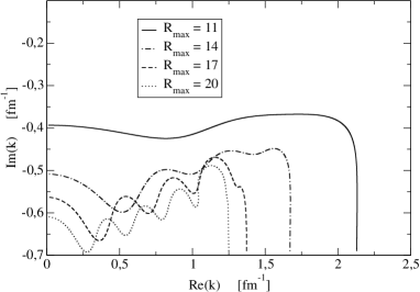
Figure 7: $n=7$ resonance trajectories for the WS potential cut off at different $R_{\rm max}$ values.

V Summary

We can summarize the results as follows.

The strange behavior of the antibound basis state found in Ref. [Lov04] is explained by its normalized radial wave function being imaginary. Except for $n=0$, the poles occur pairwise, and there is a range of potential depths in which there are two antibound states of the same node number: one below, and the other above the coalescence point. It has been shown that the antibound states lying below the coalescence points are real, while those above are imaginary. This seems to be a general property of antibound wave functions. The antibound states may be included in an orthonormal basis. Numerical examples show that even those that belong to the same node number are orthogonal to each other.

The pole belonging to node number $n=0$ is an exception; it starts (with an infinitesimally small attractive potential) as an antibound state, and becomes bound when the potential is deepened, without ever passing into the resonance region. The behavior of all other poles show similarity to the $l>0$ case [ra11] : the real parts of the starting points of the resonance trajectories (near potential zero) are inversely proportional to the potential range. For the WS potential, this range is to be identified with the cutoff radius. For the WS potential the pole trajectories, including the positions of the antibound states, depend on the cutoff radius, and the higher the node number, the stronger the dependence is. Thus, without discrediting the use of the WS potential in representing the nucleus in bound-state or scattering problems, this paper cautions against its indiscriminate use to represent broad resonances or antibound states.

References

- (1) T. Berggren, Nucl. Phys. A109, 265 (1968).
- (2) N. Michel, W. Nazarewicz, M. Ploszajczak and T. Vertse, J. Phys. G: Nucl. Part. Phys. 36, 013101 (2009).
- (3) H. Masui, S. Aoyama, T. Myo, K. Kato, K. Ikeda, Nucl. Phys., A 673, 207 (2000).
- (4) R. G. Lovas, J. Zs. Mezei, T. Vertse, A New Era of Nuclear Structure Physics, Proc. Int. Symp.,Kurokawa Village, Niigata, Japan, Eds. Y. Suzuki, S. Ohya, M. Matsuo, et al., New Jersey etc, World Scientific 141 (2004).
- (5) R. Id Betan, R. J. Liotta, N. Sandulescu, T. Vertse, Physics Lett. B 584, 48 (2004).
- (6) R. Id Betan, R. J. Liotta, N. Sandulescu, T. Vertse, R. Wyss, Phys. Rev. C 72, 054322 (2005).
- (7) Z. X. Xu, R. J. Liotta, C. Qi, T. Roger, P. Roussel-Chomaz, H. Savajols, R. Wyss, Nucl. Phys. A 850, 53 (2011).
- (8) P. Salamon, and T. Vertse, Phys. Rev. C 77, 037302 (2008).
- (9) A. Rácz, P. Salamon, and T. Vertse, Phys. Rev. C 84, 037602 (2011).
- (10) Gy. Bencze, Commentationes Physico-Mathematicae, 31, 4 (1966).
- (11) H. M. Nussenzveig, Nucl. Phys. 11, 499 (1959).
- (12) P. Curutchet, T. Vertse, and R. J. Liotta, Phys. Rev. C 39, 1020 (1989).
- (13) N. Hokkyo, Prog. Theor. Phys., 33, 1116 (1965).
- (14) B. Gyarmati, T. Vertse, Nucl. Phys. A160, 423 (1971).
- (15) T. Vertse, P. Curutchet, and R. J. Liotta, Resonances The Unifying Route Towards the Formulation of Dynamical Processes, Eds. E Brändas N. Elander, Lecture Notes in Physics 325 179 (1987).
- (16) T. Vertse, P. Curutchet, R. J. Liotta, and J. Bang, Acta Phys. Hung. 65, 305 (1989).
- (17) T. Vertse, K. F. Pál, Z. Balogh, Comput. Phys. Commun. 27, 309 (1982).
- (18) L. Gr. Ixaru, M. Rizea, T. Vertse, Comput. Phys. Commun. 85, 217(1995).
- (19) L. Gr. Ixaru, Numerical Methods for Differential Equations and Applications, D. Reidel, Publ. Comp., Dordrecht/Boston/Lancaster, 1984.
- (20) R. G. Newton, Scattering Theory of Waves and Particles, Springer Verl., New York Inc., 1982.
- (21) I. Borbély, T. Vertse, Comput. Phys. Commun. 86, 61 (1995).
- (22) J. Bang, S. N. Ershov, F. A. Gareev, and G. S. Kazacha, Nucl. Phys. A339, 89 (1980).