Partial resolution of complex cones over Fano ${\cal B}$

Abstract

In our recent paper arXiv:1108.2387, we systematized inverse algorithm to obtain quiver gauge theory living on the M2-branes probing the singularities of special kind of Calabi-Yau four-folds which were complex cones over toric Fano ${\mbox{$\mathbb{P}$}}^{3}$, ${\cal B}_{1}$, ${\cal B}_{2}$, ${\cal B}_{3}$. These quiver gauge theories cannot be given a dimer tiling presentation. We use the method of partial resolution to show that the toric data of ${\mbox{$\mathbb{C}$}}^{4}$ and Fano ${\mbox{$\mathbb{P}$}}^{3}$ can be embedded inside the toric data of Fano ${\cal B}$ theories. This method indirectly justifies that the two node quiver Chern-Simons theories corresponding to ${\mbox{$\mathbb{C}$}}^{4}$, Fano ${\mbox{$\mathbb{P}$}}^{3}$ and their orbifolds can be obtained by higgsing matter fields of the three node parent quiver corresponding to Fano ${\cal B}_{1},{\cal B}_{2},{\cal B}_{3},{\cal B}_{4}$ three-folds.

1 Introduction

Initial works of Bagger-Lambert[1, 2, 3] followed by Gustavsson[4, 5], Raamsdonk[6] and Aharony-Bergman-Jafferis-Maldacena (ABJM)[7] led to a flurry of interesting papers during the last four years between supersymmetric Chern-Simons gauge theory on coincident $M2$-branes at the tip of Calabi-Yau four folds and their string duals. In a review article[8], these developments are discussed in detail.

Martelli et al[9] discussed the gauge-gravity correspondence ($AdS_{4}/CFT_{3}$) for some supersymmetric Chern-Simons theories with a quiver diagram description. Earlier works of Hanany et al in the context of Calabi-Yau three-folds[10] called forward algorithm, can be extended to obtain Calabi-Yau four-fold toric data from $2+1$ dimensional quiver supersymmetric Chern-Simons theories.

An elegant combinatorial approach called dimer tilings[11, 12] which gives both the toric data and the corresponding quiver gauge theories was generalised to study quiver Chern-Simons theories[13, 14, 15, 16, 17, 18, 19, 20]. However, the dimer tiling approach is applicable for only a class of quiver gauge theories with $m$-matter fields, $r$ gauge group nodes and $N_{W}$ number of terms in the superpotential $W$ satisfying $r-m+N_{W}=0$. The Chern-Simons (CS) levels of the $r$-nodes can be denoted by the vector $\vec{k}=(k_{1},k_{2},\ldots k_{r})$.

One of the challenging problems was to determine quiver gauge theories corresponding to 18 toric Fano three-folds. A Fano variety in $d$-complex dimension is characterized by positive curvature and one can construct the CY ($d+1$)-fold by taking a complex cone over it. If the Fano variety is toric, the Calabi-Yau constructed from it will also be toric and one can attempt to find the dual quiver gauge theories. In 2 complex dimensions, there are 5 toric Fano 2-folds which are: zeroth Hirzebruch surface $\mathbb{F}_{0}$ and the del Pezzo surfaces $dP_{0}$, $dP_{1}$, $dP_{2}$, $dP_{3}$. The quiver gauge theories living on D3 branes probing the toric CY 3-folds obtained from these 5 Fano 2-folds have been studied in the literature[10]. Moving on to 3 complex dimensions, there are 18 toric Fano 3-folds[21, 22] with nomenclature (as used in [20]) Fanos $\mathbb{P}^{3}$, ${\cal{B}}_{1}$, ${\cal{B}}_{2}$, ${\cal{B}}_{3}$, ${\cal{B}}_{4}$, ${\cal{C}}_{1}$, ${\cal{C}}_{2}$, ${\cal{C}}_{3}$, ${\cal{C}}_{4}$, ${\cal{C}}_{5}$, ${\cal{D}}_{1}$, ${\cal{D}}_{2}$, ${\cal{E}}_{1}$, ${\cal{E}}_{2}$, ${\cal{E}}_{3}$, ${\cal{E}}_{4}$, ${\cal{F}}_{1}$, ${\cal{F}}_{2}$. The next problem was to obtain the quiver CS theory living on the M2 branes probing the toric CY 4-folds obtained from these 18 Fano 3-folds.

From the forward algorithm and dimer tiling method, quiver gauge theories corresponding to fourteen of the toric Fanos ${\cal{B}}_{4}$, ${\cal{C}}_{1}$, ${\cal{C}}_{2}$, ${\cal{C}}_{3}$, ${\cal{C}}_{4}$, ${\cal{C}}_{5}$, ${\cal{D}}_{1}$, ${\cal{D}}_{2}$, ${\cal{E}}_{1}$, ${\cal{E}}_{2}$, ${\cal{E}}_{3}$, ${\cal{E}}_{4}$, ${\cal{F}}_{1}$, ${\cal{F}}_{2}$ were determined[20]. In Ref.[23], we attempted the inverse algorithm of obtaining the quiver gauge theories for the remaining four Fano 3-folds $\mathbb{P}^{3}$, ${\cal{B}}_{1}$, ${\cal{B}}_{2}$, ${\cal{B}}_{3}$. As expected, these quiver gauge theories do not satisfy $r-m+N_{W}=0$ confirming that they cannot be given dimer tiling presentation.

The next immediate question is to understand the embeddings inside the toric Fano ${\cal B}$ three-folds by the method of partial resolution. In particular, we would like to obtain the quiver Chern-Simons theory corresponding to Fano ${\mbox{$\mathbb{P}$}}^{3}$ by partial resolution of Fano ${\cal B}$ three-folds.

Alternatively, we could determine embeddings from higgsing approach[24, 19, 25]: For the quivers with $r$ nodes (usually called parent theories) which admit dimer tiling, we could higgsize some matter fields and obtain quivers with $r-1$ nodes (called daughter theories). Suppose we give a vacuum expectation value (VEV) to a bifundamental matter field $X_{ab}$ where the subscript denotes that the matter field is charged $+1$ with respect to node $a$ with Chern-Simons level $k_{a}$ and charged $-1$ with respect to node $b$ with Chern-Simons level $k_{b}$. This results in coalescing of two nodes $a$ and $b$ into a node with Chern-Simons level $k_{a}+k_{b}$. Higgsing of the three node quiver corresponding to a toric Fano ${\cal B}_{4}$ was discussed from dimer tilings in Ref.[19]. In fact, the daughter theories corresponds to either phase II of ${\mbox{$\mathbb{C}$}}^{4}$ or phase I of ${\mbox{$\mathbb{C}$}}^{2}/{\mbox{$\mathbb{Z}$}}_{2}\times{\mbox{$\mathbb{C}$}}^{2}$ depending upon which bifundamental field was given VEV.

Another approach of higgsing called the algebraic method[24] has been applied on parent quivers[25] corresponding to some toric Fano 3-folds. We shall present the algebraic higgsing for Fano ${\cal B}_{4}$ and show that the toric data corresponding to daughter theories has to be ${\mbox{$\mathbb{C}$}}^{4}$ or orbifolds of ${\mbox{$\mathbb{C}$}}^{4}$. We will also study the method of partial resolution[10] and obtain the ${\mbox{$\mathbb{C}$}}^{4}$ toric data for the daughter theories.

For the $3$-node quivers corresponding to Fano ${\cal B}_{1},{\cal B}_{2}$ and ${\cal B}_{3}$, which do not admit dimer tiling presentation, we have to obtain daughter theories by the algebraic higgsing method[25] or the partial resolution method[10]. We shall show that the algebraic higgsing on these $3$-node quivers always gives ${\mbox{$\mathbb{C}$}}^{4}$ or orbifolds of ${\mbox{$\mathbb{C}$}}^{4}$. We also study the method of partial resolution to check whether the approach gives more information about the embedded theories. Interestingly this method shows that the toric data of Fano ${\mbox{$\mathbb{P}$}}^{3}$ or its orbifolds is embedded in the toric data of Fano ${\cal B}_{2}$ and Fano ${\cal B}_{3}$.

The plan of the paper is as follows: In section 2, we briefly review the well known 2-node quiver Chern-Simons theory with four matter fields and their toric data. In section 3, we will first perform the higgsing of toric Fano ${\cal B}_{4}$ using the algebraic method and determine the daughter quiver theories with $2$-nodes. Finally, we show that the partial resolution method gives ${\mbox{$\mathbb{C}$}}^{4}$ toric data. In section 4, we will briefly present the necessary data of the quiver corresponding to Fano ${\cal B}_{3}$. Then we study the algebraic higgsing and the method of partial resolution for Fano ${\cal B}_{3}$. Particularly, we show that the algebraic higgsing gives ${\mbox{$\mathbb{C}$}}^{4}$ or orbifolds of ${\mbox{$\mathbb{C}$}}^{4}$ whereas the method of partial resolution gives non-trivial embeddings inside Fano ${\cal B}_{3}$. In section 5, we study the method of partial resolution for Fano ${\cal B}_{2}$. We present the results of partial resolution of Fano ${\cal B}_{1}$ in section 6 . We summarize and discuss some open problems in section 7.

2 Two-node quiver Chern-Simons theories

Our aim is to study partial resolution of toric data corresponding to $3$-node parent quiver resulting in a toric data corresponding to a $2$-node daughter quiver. So, in this section we will briefly recapitulate the $2$-node quivers with four matter fields corresponding to toric data of ${\mbox{$\mathbb{C}$}}^{4}$, orbifolds of ${\mbox{$\mathbb{C}$}}^{4}$ and Fano ${\mbox{$\mathbb{P}$}}^{3}$. There can be three possible quivers:

1. Theory with 4 bi-fundamental matter fields $X_{12}^{i}$ and $X_{21}^{i}$ (where $i=1,2$), with CS levels ($k,-k$) and the superpotential $W={\rm Tr}[\epsilon_{ij}X_{12}^{1}X_{21}^{i}X_{12}^{2}X_{21}^{j}]$. For the abelian groups, $W=0$. The quiver diagram is shown in figure 1. This theory admits tiling and the corresponding toric data is[18]:

   $${\cal{G}}_{a}(k)=\left(\begin{array}[]{cccc}p_{1}&p_{2}&p_{3}&p_{4}\\ \hline\cr 1&1&1&1\\ -1&0&-1&0\\ 0&-1&-1&0\\ 0&0&k&0\end{array}\right)~{}.$$ (2.1)

   The charge matrix $Q_{a}$ for this theory given by $Q_{a}.{{\cal{G}}^{T}_{a}(k)}=0$ is trivial, $Q_{a}=0$. This theory is $\mbox{$\mathbb{Z}$}_{k}$ orbifold of $\mbox{$\mathbb{C}$}^{4}$, denoted as $\mbox{$\mathbb{C}$}^{4}/\mbox{$\mathbb{Z}$}_{k}$. For $k=1$, i.e, when the CS-levels of the theory is (1, -1), there is no orbifolding action and this theory in the literature is known as Phase-I of $\mbox{$\mathbb{C}$}^{4}$[18].

   

   Figure 1: Quiver diagram (a)

2. Theory with 2 adjoints $\phi_{2}^{1},\phi_{2}^{2}$ present at the same node (say node 2) and two bifundamentals $X_{12},X_{21}$, with CS-levels ($k,-k$). Abelian $W$ of this theory is again zero with non-abelian superpotential $W={\rm Tr}[X_{12}[\phi_{2}^{1},\phi_{2}^{2}]X_{21}]$. The quiver diagram is shown in figure 2. This theory also admits tiling and the toric data for this theory is[18]:

   $${\cal{G}}_{b}(k)=\left(\begin{array}[]{cccc}p_{1}&p_{2}&p_{3}&p_{4}\\ \hline\cr 1&1&1&1\\ 1&0&1&0\\ 0&-1&0&0\\ 0&0&k&0\end{array}\right)~{}.$$ (2.2)

   The charge matrix $Q_{b}$ of this theory given by $Q_{b}.{{\cal{G}}^{T}_{b}(k)}=0$ is also trivial, $Q_{b}=0$. This is $\left(\mbox{$\mathbb{C}$}^{2}/\mbox{$\mathbb{Z}$}_{k}\right)\times\mbox{$\mathbb{C}$}^{2}$ theory. For $k=1$, this theory is known as Phase-II of $\mbox{$\mathbb{C}$}^{4}$.

   It is pertinent to spell out the following obvious facts:
   (i) We can deduce that the two quiver theories are distinct for $k\neq 1$ because the toric data of the two theories (${\cal{G}}_{a}(k)$ and ${\cal{G}}_{b}(k)$) are not related by any $GL(4,\mbox{$\mathbb{Z}$})$ transformation.
   (ii) When there is no orbifolding- i.e., $k=1$, both the theories are same upto some $GL(4,\mbox{$\mathbb{Z}$})$ transformation. Hence these theories are actually just the phases of $\mbox{$\mathbb{C}$}^{4}$ theory, known as Phase-I and Phase-II of $\mbox{$\mathbb{C}$}^{4}$ respectively.

   

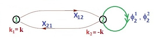
   Figure 2: Quiver diagram (b)

3. Theory with 2 bifundamentals $X_{12}$, $X_{21}$ and adjoints $\phi_{1}$, $\phi_{2}$ at two different nodes with trivial $W=0$. The quiver of this theory is shown in figure 3. This theory does not admit tiling and was first obtained using the inverse algorithm in[23], which was identified as the Fano $\mathbb{P}^{3}$ theory.

   However, we cannot determine the CS levels from the inverse algorithm[23] for all the three $2$-node quiver theories. From the tiling description, we can obtain the CS levels for the quiver diagrams (a) and (b). Comparing the inverse algorithm of the three theories, we had inferred that the theory corresponding to Fano ${\mbox{$\mathbb{P}$}}^{3}$ could have CS-levels $(4,-4)$. As we do not know any method of determining the actual CS levels, the theory shown in quiver diagram (c) with $k=1$ could be Fano ${\mbox{$\mathbb{P}$}}^{3}$ theory.

   A possible choice of toric data for the theory shown in figure 3 can be:

   $${\cal{G}}_{c}(k)=\left(\begin{array}[]{ccccc}p_{1}&p_{2}&p_{3}&p_{4}&p_{5}\\ \hline\cr 1&1&1&1&1\\ 1&-1&0&0&0\\ 0&1&-1&0&0\\ 0&0&k&-k&0\end{array}\right)~{},$$ (2.3)

   which is related to the toric data ${\cal G}_{c}(k=1)\equiv{\cal{G}}_{\mbox{$\mathbb{P}$}^{3}}$ by $GL(4,{\mbox{$\mathbb{Z}$}})$ transformation ${\cal T}(k)$, such that the determinant of $\cal T$ is $k$.

The charge matrix $Q_{c}(k)$ of this theory given by $Q_{c}(k).{{\cal{G}}_{c}(k)}^{T}=0$ consists only of $Q_{F}$ and is given by[23]:

$$Q_{c}(k)=Q_{F}^{{\mbox{$\mathbb{P}$}}^{3}}=(1,1,1,1,-4)~{},$$ (2.4)

for all $k$. This indicates that the charge $Q_{F}$ will not be able to detect the orbifolding ${\mbox{$\mathbb{Z}$}}_{k}$.

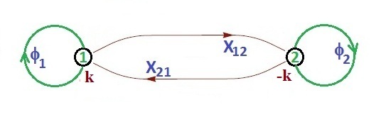
Figure 3: Quiver diagram (c)

We would like to see these Calabi-Yau 4-folds, particularly Fano ${\mbox{$\mathbb{P}$}}^{3}$, as embeddings inside Calabi-Yau 4-fold toric data corresponding to some $3$-node quivers. In the following section, we will extensively discuss the $3$-node quiver corresponding to Fano ${\cal B}_{4}$ which admits dimer tiling. Higgsing of the theory corresponding to Fano ${\cal B}_{4}$[19], from the tiling approach, has shown that the daughter theories are only quiver diagram (b). From the method of algebraic higgsing we get the toric data to be ${\mbox{$\mathbb{C}$}}^{4}$ and orbifolds of ${\mbox{$\mathbb{C}$}}^{4}$ whereas partial resolution gives toric data of $\mbox{$\mathbb{C}$}^{4}$. This will set the necessary tools and notations for studying the embeddings inside other three Fano ${\cal B}_{i}$’s in the later sections.

3 Fano ${\cal B}_{4}$

The quiver corresponding to the complex cone over Fano ${\cal B}_{4}$ is a theory with $3$-nodes and $9$ bifundamental fields $X_{12}^{i}$, $X_{23}^{i}$, $X_{31}^{i}$, where $i=1,2,3$. This theory admits tiling and is known in the literature as Fano ${\cal B}_{4}$ or $M^{1,1,1}$ theory with CS-levels $\vec{k}=(k_{1},k_{2},k_{3})=(1,-2,1)$ [20]. The quiver diagram for this theory is shown in figure 4.

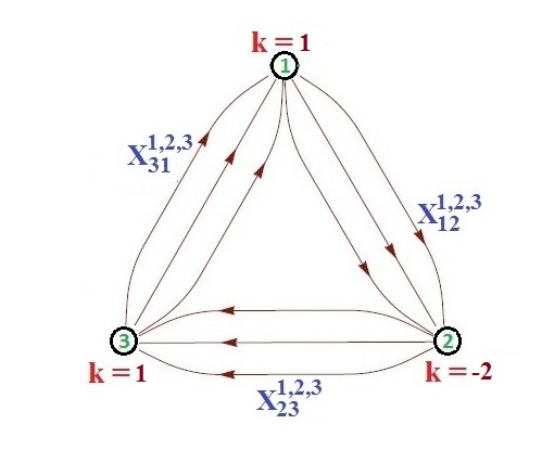
Figure 4: Quiver Diagram for Fano ${\cal B}_{4}$

The superpotential of the theory is given by:

$$W={\rm Tr}\left[\epsilon_{ijk}X_{12}^{i}X_{23}^{j}X_{31}^{k}\right]~{}.$$ (3.1)

The incidence matrix of this theory is given by:

$$d=\left(\begin{array}[]{c|ccccccccc}&X_{12}^{1}&X_{12}^{2}&X_{12}^{3}&X_{23}^{1}&X_{23}^{2}&X_{23}^{3}&X_{31}^{1}&X_{31}^{2}&X_{31}^{3}\\ \hline\cr G=1&1&1&1&0&0&0&-1&-1&-1\\ G=2&-1&-1&-1&1&1&1&0&0&0\\ G=3&0&0&0&-1&-1&-1&1&1&1\end{array}\right)~{},$$ (3.2)

where the rows indicate the gauge groups or the nodes in the quiver, and columns indicate the matter fields.

The projected charge matrix ($\Delta$) will consist of a single row whose elements will be given by

$$\Delta_{i}=k_{2}d_{1i}-k_{1}d_{2i}=-(2d_{1i}+d_{2i})~{}.$$ (3.3)

Hence, $\Delta$ matrix will be given by:

$$\Delta=\left(\begin{array}[]{ccccccccc}X_{12}^{1}&X_{12}^{2}&X_{12}^{3}&X_{23}^{1}&X_{23}^{2}&X_{23}^{3}&X_{31}^{1}&X_{31}^{2}&X_{31}^{3}\\ \hline\cr-1&-1&-1&-1&-1&-1&2&2&2\end{array}\right)~{}.$$ (3.4)

From the superpotential $W$ (3.1), one can find the $F$-term constraints given by the set of equations $\left\{\partial W/\partial X_{i}=0\right\}$, which means that the matter fields $X_{i}$’s can be written in terms of 5 independent $v$-fields, and the relation between them can be encoded in a matrix $K$. The matrix $K$ and its dual matrix $T$ are given as:

$$K=\left(\begin{array}[]{c|ccccc}{}\hfil&v_{1}&v_{2}&v_{3}&v_{4}&v_{5}\\ \hline\cr X_{12}^{(1)}&0&0&1&0&0\\ X_{12}^{(2)}&0&0&1&0&1\\ X_{12}^{(3)}&0&0&1&1&0\\ X_{23}^{(1)}&0&1&0&0&0\\ X_{23}^{(2)}&0&1&0&0&1\\ X_{23}^{(3)}&0&1&0&1&0\\ X_{31}^{(1)}&1&0&0&0&0\\ X_{31}^{(2)}&1&0&0&0&1\\ X_{31}^{(3)}&1&0&0&1&0\end{array}\right)~{};~{}T=\begin{pmatrix}1&0&0&0&0&1\cr 1&0&0&0&1&0\cr 1&0&0&1&0&0\cr-1&0&1&0&0&0\cr-1&1&0&0&0&0\end{pmatrix}~{}.$$ (3.5)

From $K$ and $T$, we can write the matrix $P=K.T$. The entries of the matrix $P$ are all non-negative and it gives the relation of the matter fields $X_{i}$’s with the GLSM fields $p_{i}$’s:

$$P=\left(\begin{array}[]{c|cccccc}&p_{1}&p_{2}&p_{3}&p_{4}&p_{5}&p_{6}\\ \hline\cr X_{12}^{1}&1&0&0&1&0&0\\ X_{12}^{2}&0&1&0&1&0&0\\ X_{12}^{3}&0&0&1&1&0&0\\ X_{23}^{1}&1&0&0&0&1&0\\ X_{23}^{2}&0&1&0&0&1&0\\ X_{23}^{3}&0&0&1&0&1&0\\ X_{31}^{1}&1&0&0&0&0&1\\ X_{31}^{2}&0&1&0&0&0&1\\ X_{31}^{3}&0&0&1&0&0&1\end{array}\right)~{}.$$ (3.6)

The $Q_{F}$ charge matrix is given by the nullspace of $P$:

$$Q_{F}=\left(\begin{array}[]{cccccc}1&1&1&-1&-1&-1\end{array}\right)~{}.$$ (3.7)

The steps done so far in obtaining $P$-matrix and the charge $Q_{F}$ are independent of the CS levels. The information about CS levels is contained only in the charge $Q_{D}$ matrix which is a single row obeying the symmetry of the Calabi-Yau which is given as:

$$Q_{D}=P.\Delta^{t}=\left[\begin{array}[]{cccccc}0&0&0&1&1&-2\end{array}\right]~{}.$$ (3.8)

The total charge matrix can be obtained by concatenating (3.7) and (3.8) in a single matrix $Q$:

$$Q=\left(\begin{array}[]{c}Q_{F}\\ \hline\cr Q_{D}\end{array}\right)=\left(\begin{array}[]{cccccc}1&1&1&-1&-1&-1\\ \hline\cr 0&0&0&1&1&-2\end{array}\right)~{}.$$ (3.9)

The toric data of this theory is[20]:

$${\cal{G}}(1,-2,1)=\left(\begin{array}[]{cccccc}p_{1}&p_{2}&p_{3}&p_{4}&p_{5}&p_{6}\\ \hline\cr 1&1&1&1&1&1\\ 1&-1&0&0&0&0\\ 0&1&-1&0&0&0\\ 0&0&0&1&-1&0\end{array}\right)~{}.$$ (3.10)

Suppose we rescale the levels of this theory as $(k_{1},k_{2},k_{3})=(n,-2n,n)$, where $n$ is some non-zero integer. Since this theory admits brane tiling description, the toric data for the scaled levels $(n,-2n,n)$ can be readily obtained from the Kastelyn matrix method[20]. The toric data is dependent on the scale $n$ and is given below:

$${\cal{G}}(n,-2n,n)=\left(\begin{array}[]{cccccc}1&1&1&1&1&1\\ 1&0&-1&0&0&0\\ -1&1&0&0&0&0\\ 0&0&0&n&-n&0\end{array}\right)$$ (3.11)

Unfortunately, when we perform forward algorithm for the scaled CS levels $(n,-2n,n)$ we see from eqns.(3.3,3.8) that $Q_{D}$ gets scaled by factor $n$ but $Q_{F}$ remains unchanged. Clearly, the toric data ${\cal{G}}(1,-2,1)$ obtained as the null space of total charge matrix $Q$ i.e ${\cal{G}}.Q^{t}=0$ is still satisfied by $Q^{t}=\left(\begin{matrix}Q_{F}^{t}&nQ_{D}^{t}\end{matrix}\right)$.

Equivalently, the toric data ${\cal G}$ obtained from forward algorithm has scaling ambiquity of any of the rows and hence not unique. These arguments on ambiquity of $\cal G$, scaling of $Q_{D}$ and $\Delta$ under $\vec{k}\rightarrow n\vec{k}$ holds for inverse algorithm as well. Following the works on orbifolds of $\mbox{$\mathbb{C}$}^{4}$, it is a well known fact that ${\cal{G}}(n,-2n,n)$ obtained from tiling must be the $\mathbb{Z}_{n}$ orbifold of ${\cal{G}}(1,-2,1)$ theory. The two toric datas are related by a $GL(4,\mathbb{Z})$ transformation ${\cal{T}}$ as:

$${\cal{G}}(n,-2n,n)={\cal{T}}.{\cal{G}}(1,-2,1)~{},$$ (3.12)

where,

$${\cal{T}}=\left(\begin{array}[]{cccc}1&0&0&0\\ 0&1&0&0\\ 0&0&1&0\\ 0&0&0&n\end{array}\right)~{}.$$ (3.13)

Here $|det({\cal{T}})|=n$, which means that the volume of ${\cal{G}}(n,-2n,n)$ theory is $n$ times that of ${\cal{G}}(1,-2,1)$ implying that the former theory is $\mathbb{Z}_{n}$ orbifold of latter theory. This orbifolding action, also scaling of CS levels, is explainable only for those theories which admit tiling. From our forward algorithm discussion, we have explicitly seen that the scaling of CS levels does not give the orbifolding information in the toric data. Reconciling with tiling results, we will hitherto use that fact that the scaling of CS levels represents ${\mbox{$\mathbb{Z}$}}_{n}$ orbifolding of all theories which may or may not admit tiling.

From the tiling approach, higgsing of the quiver diagram in figure 4 has been presented in detail in Ref.[19]. In particular, we can obtain daughter quivers in figure 2 corresponding to ${\mbox{$\mathbb{C}$}}^{4}$ and orbifolds of ${\mbox{$\mathbb{C}$}}^{4}$. We will now study the algebraic approach of higgsing which will be applicable for other quivers that do not admit dimer tiling presentation.

3.1 Algebraic higgsing

We attempt the higgsing of Fano ${\cal B}_{4}$ theory to obtain one of the 2 nodes theories discussed in section 2. In algebraic higgsing, we choose some matter field, say $X_{i}$ and give a non zero VEV to it. Giving a VEV makes the matter field massive and hence removed from the quiver. However, in the process of giving VEV, all those GLSM $p_{j}$ fields which contain the matter field $X_{i}$ also become massive and hence must be removed. To do this, we delete the $i$-th row from the $P$ matrix which corresponds to the matter field $X_{i}$ and also, we remove all those columns ($p$-fields) which have non-zero entry corresponding to $i$-th row (and hence have become massive).

As an example, let us take the $X_{12}^{1}$ field of the ${\cal B}_{4}$ theory and give a VEV to it. Thus, from the $P$ matrix (3.6), we must remove the first row and also the columns $1$ and $4$ which correspond to the GLSM fields $p_{1},p_{4}$ which contain the $X_{12}^{1}$ field. After giving VEV to the $X_{12}^{1}$ field, the nodes 1 and 2 in the figure 4 are collapsed giving a 2 node daughter theory with CS levels $(1,-1)$. Removal of the corresponding row and columns in eqn.(3.6) will give the following reduced $P$-matrix:

$$P_{r}=\left(\begin{array}[]{c|cccc}&p_{2}&p_{3}&p_{5}&p_{6}\\ \hline\cr X_{12}^{2}&1&0&0&0\\ X_{12}^{3}&0&1&0&0\\ X_{23}^{1}&0&0&1&0\\ X_{23}^{2}&1&0&1&0\\ X_{23}^{3}&0&1&1&0\\ X_{31}^{1}&0&0&0&1\\ X_{31}^{2}&1&0&0&1\\ X_{31}^{3}&0&1&0&1\end{array}\right)~{}.$$ (3.14)

The nullspace of this matrix gives the reduced charge matrix $Q_{F_{r}}=0$. Thus, we see that the $Q_{F_{r}}$ of the daughter theory is trivial. The quivers (a) and (b) listed in section 2 have $Q_{F}=0$. So, algebraic higgsing can give daughter quivers (a) as well as quiver (b) with CS levels $(1,-1)$.

By giving VEV to any other matter fields, we have checked that we get the same trivial $Q_{F_{r}}=0$. This suggests that the algebraic higgsing of the parent quiver corresponding to Fano ${\cal B}_{4}$ will give quivers corresponding to ${\mbox{$\mathbb{C}$}}^{4}$ and orbifolds of ${\mbox{$\mathbb{C}$}}^{4}$. It must be mentioned at this point that the algebraic higgsing of Fano ${\cal B}_{1}$, ${\cal B}_{2}$, ${\cal B}_{3}$ also gives a daughter theory with trivial $Q_{F}$. So, the algebraic higgsing tells that only $\mbox{$\mathbb{C}$}^{4}$ or the orbifolds of $\mbox{$\mathbb{C}$}^{4}$ are embedded inside Fano ${\cal B}_{1},{\cal B}_{2},{\cal B}_{3},{\cal B}_{4}$. It may be possible that we may get non-trivial $Q_{F}$ from the method of partial resolution. So, we shall study the method of partial resolution for Fano ${\cal B}_{4}$ toric data.

3.2 Partial Resolution

In partial resolution, we try to remove the points from the toric diagram. The resulting toric diagram corresponds to some daughter theory which is embedded in the parent theory. From the toric diagram of ${\cal B}_{4}$, we will remove some points which amounts to removing the corresponding columns (or the corresponding $p$-fields) from the toric data ${\cal{G}}$. Next, we will check whether this reduced toric data (denoted as ${\cal{G}}_{r}$), which is obtained by removing the columns from original ${\cal{G}}$, is related to any of the toric data of the 2-node theories.

Take the toric data ${\cal{G}}$ of Fano ${\cal B}_{4}$ in eqn.(3.10). We see that if we remove the points $p_{1}$ and $p_{4}$, we get the reduced toric data

$${\cal{G}}_{r}=\left(\begin{array}[]{cccc}1&1&1&1\\ -1&0&0&0\\ 1&-1&0&0\\ 0&0&-1&0\end{array}\right)~{}.$$ (3.15)

This reduced toric data (3.15) is equivalent to the toric datas ${\cal{G}}_{a}(k=1)$ (2.1) and ${\cal{G}}_{b}(k=1)$ (2.2):

$${\cal{G}}_{a}(k=1)=\left(\begin{array}[]{cccc}1&0&0&0\\ 0&1&0&1\\ 0&1&1&1\\ 0&0&0&-1\end{array}\right)~{}.~{}{\cal{G}}_{r}~{},$$ (3.16)

$${\cal{G}}_{b}(k=1)=\left(\begin{array}[]{cccc}1&0&0&0\\ 0&-1&0&-1\\ 0&1&1&0\\ 0&0&0&-1\end{array}\right)~{}.~{}{\cal{G}}_{r}~{}.$$ (3.17)

Thus partial resolution of ${\cal B}_{4}$ toric data (3.10) only gives $\mbox{$\mathbb{C}$}^{4}$ toric data. Explicit coalescing of nodes in tiling/algebraic higgsing allows both $\mbox{$\mathbb{C}$}^{4}$ or $\mbox{$\mathbb{Z}$}_{2}$ orbifold of $\mbox{$\mathbb{C}$}^{4}$ whereas we get only ${\cal{G}}_{a}(k=1)$ or ${\cal{G}}_{b}(k=1)$ in the partial resolution method.

Alternatively, we can take the charge matrix $Q$ of the ${\cal B}_{4}$ theory given in eqn.(3.9) and take a linear combination and set the charge matrix elements corresponding to column $p_{1}$ and $p_{4}$ to zero as described below: Suppose that a row ($r$) of $Q$ of the daughter theory is given as some linear combination of rows ($R_{i}$) of $Q$ (3.9) of parent theory, i.e.

$$r=\sum_{i=1}^{2}(a_{i}R_{i})=(a_{1},a_{1},a_{1},-a_{1}+a_{2},-a_{1}+a_{2},-a_{1}-2a_{2})~{}.$$ (3.18)

Since we are removing $p_{1}$ and $p_{4}$ points, the corresponding columns in $r$ are set to 0 and also removed. This will give the values of $a_{1}$ and $a_{2}$, and we find that $a_{1}=a_{2}=0$. Hence, the $Q$ of the daughter theory is trivial.

We have obtained ${\cal G}_{r}$ by removing all other possible set of points in the toric data of ${\cal B}_{4}$- namely., $\left\{p_{1},p_{5}\right\}$, $\left\{p_{2},p_{4}\right\}$, $\left\{p_{2},p_{5}\right\}$, $\left\{p_{3},p_{4}\right\}$ and $\left\{p_{4},p_{5}\right\}$ and checked that they are again related by $GL(4,\mbox{$\mathbb{Z}$})$ to ${\cal{G}}_{a}(k=1)$ and ${\cal{G}}_{b}(k=1)$. For all these cases, the linear combination of the charge $Q$ matrix (3.9) with the appropriate columns removed gives $Q$ of the daughter theory to be trivial ($Q=0$). Thus we see that $\mbox{$\mathbb{C}$}^{4}$ theory is embedded in the ${\cal B}_{4}$ theory.

The quiver gauge theories corresponding to Fano ${\cal B}_{3}$ and ${\cal B}_{2}$ have non-trivial superpotential $W$[23] and hence can be described by both forward and inverse algorithm. We will briefly present in the next section, the quiver and necessary data for Fano ${\cal B}_{3}$ and study algebraic higgsing and partial resolution.

4 Fano ${\cal B}_{3}$

It is a theory with 3-nodes, 2 adjoint fields $X_{1},X_{2}$ on node-1 and 6 bifundamental fields $X_{3},X_{4},X_{5},X_{6},X_{7},X_{8}$. The quiver diagram for this theory is shown in figure 5. This theory does not admit tiling and was first studied in [23], where it was identified as the quiver gauge theory for Fano ${\cal B}_{3}$ with CS-levels (6,-6,0).

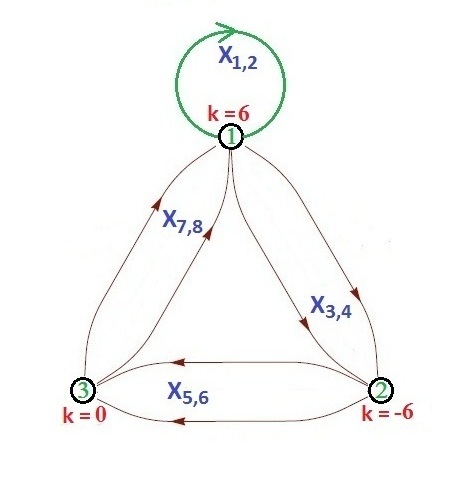
Figure 5: Quiver Diagram for Fano ${\cal B}_{3}$

The superpotential of the theory is given by:

$$W={\rm Tr}\left[\left(X_{1}X_{4}-X_{2}X_{3}\right)\left(X_{5}X_{8}-X_{6}X_{7}\right)\right]~{}.$$ (4.1)

From $W$ given in (4.1), we construct $K$, which gives $T$ and hence $P$:

$$P=\left(\begin{array}[]{c|ccccccc}&p_{1}&p_{2}&p_{3}&p_{4}&p_{5}&p_{6}&p_{7}\\ \hline\cr X_{1}&3&0&1&0&0&0&1\\ X_{2}&0&3&1&0&0&0&1\\ X_{3}&3&0&0&1&0&0&1\\ X_{4}&0&3&0&1&0&0&1\\ X_{5}&0&0&4&0&6&0&1\\ X_{6}&0&0&0&4&6&0&1\\ X_{7}&0&0&4&0&0&6&1\\ X_{8}&0&0&0&4&0&6&1\end{array}\right)~{}.$$ (4.2)

Total charge matrix $Q$ is given by:

$$Q=\left(\begin{array}[]{c}Q_{F}\\ \hline\cr Q_{D}\end{array}\right)=\left(\begin{array}[]{ccccccc}1&1&3&3&-1&-1&-6\\ 1&1&1&1&0&0&-4\\ \hline\cr 0&0&2&2&-2&0&-2\end{array}\right)~{}.$$ (4.3)

The toric data of the theory is given as [23]:

$${\cal{G}}(6,-6,0)=\left(\begin{array}[]{ccccccc}p_{1}&p_{2}&p_{3}&p_{4}&p_{5}&p_{6}&p_{7}\\ \hline\cr 1&1&1&1&1&1&1\\ 1&-1&0&0&0&0&0\\ 0&0&1&-1&0&0&0\\ 0&1&0&-1&-1&-1&0\end{array}\right)~{}.$$ (4.4)

Similar to Fano ${\cal B}_{4}$ theory, if we rescale the levels here to $(k_{1},k_{2},k_{3})=(6n,-6n,0)$, where $n$ is some non-zero integer, we can write the toric data which has information about this scaling. Note that this theory does not admit tiling and the forward/inverse algorithm does not give an explicit dependence of ${\cal{G}}(6n,-6n,0)$ on $n$, but there is a scaling ambiquity of any row of toric data. A choice of the toric data will be

$${\cal{G}}(6n,-6n,0)=\left(\begin{array}[]{ccccccc}1&1&1&1&1&1&1\\ 1&-1&0&0&0&0&0\\ 0&0&1&-1&0&0&0\\ 0&n&0&-n&-n&-n&0\end{array}\right)$$ (4.5)

This toric data is related to that of ${\cal{G}}(6,-6,0)$ by a volume factor $n$ and hence represents the $\mathbb{Z}_{n}$ orbifolding:

$${\cal{G}}(6n,-6n,0)=\left(\begin{array}[]{cccc}1&0&0&0\\ 0&1&0&0\\ 0&0&1&0\\ 0&0&0&n\end{array}\right).{\cal{G}}(6,-6,0)$$ (4.6)

We will now study algebraic higgsing and obtain two-node daughter quivers.

4.1 Algebraic higgsing

If we give a VEV to any of the $X_{i}$ fields, thereby removing the corresponding row and columns from the $P$-matrix (4.2), we see that we get a reduced matrix ($P_{r}$), whose null space (${Q_{F}}_{r}$) is always trivial. Starting from the parent quiver as shown in figure 5, we see that the non-trivial CS levels of the 2-node daughter quiver to be $(6,-6)$. Thus, we can only say that the higgsing of the $\mbox{$\mathbb{Z}$}_{n}$ orbifolds of Fano ${\cal B}_{3}$ theory will give $\mbox{$\mathbb{C}$}^{4}/\mbox{$\mathbb{Z}$}_{6n}$ as the daughter theory. Moreover, we see that the last column ($p_{7}$) of P matrix (4.2) which corresponds to the internal point in the toric diagram of Fano ${\cal B}_{3}$ will always be removed because it contains all the matter fields. So, this method cannot give a daughter theory corresponding to Fano ${\mbox{$\mathbb{P}$}}^{3}$ which has an internal point in the toric diagram. Hence we are forced to study the method of partial resolution to check whether toric Fano ${\mbox{$\mathbb{P}$}}^{3}$ is embedded inside ${\cal B}_{3}$ Fano.

4.2 Partial Resolution

Here, we do the partial resolution of Fano ${\cal B}_{3}$ theory and also check whether we get non-trivial charge $Q$ for the daughter theory.

4.2.1 Embedding of Fano $\mbox{$\mathbb{P}$}^{3}$ inside Fano ${\cal B}_{3}$

It is interesting to see that the method of partial resolution does embed the toric Fano ${\mbox{$\mathbb{P}$}}^{3}$ inside Fano ${\cal B}_{3}$ giving the correct $Q_{F}$ (2.4). Hence we can claim that this method gives more information than algebraic higgsing for quiver which do not admit dimer tiling presentation. Suppose we remove the points $\left\{p_{5},p_{6}\right\}$ from the ${\cal{G}}$ (4.4), we get a reduced toric data

$${\cal{G}}_{r}=\left(\begin{array}[]{ccccc}p_{1}&p_{2}&p_{3}&p_{4}&p_{7}\\ \hline\cr 1&1&1&1&1\\ 1&-1&0&0&0\\ 0&0&1&-1&0\\ 0&1&0&-1&0\end{array}\right)$$ (4.7)

and the toric data ${\cal{G}}_{\mbox{$\mathbb{P}$}^{3}}\equiv{\cal G}_{c}(k=1)$ (2.3) is related to ${\cal{G}}_{r}$ by a $GL(4,\mbox{$\mathbb{Z}$})$ transformation:

$${\cal{G}}_{\mbox{$\mathbb{P}$}^{3}}=\left(\begin{array}[]{cccc}1&0&0&0\\ 0&1&0&0\\ 0&0&-1&1\\ 0&0&1&0\end{array}\right).~{}{\cal{G}}_{r}~{}.$$ (4.8)

A row ($r$) of $Q$ of the daughter theory will be given as linear combination of rows ($R_{i}$) of $Q$ (4.3) i.e,

$$r=\sum_{i=1}^{3}(a_{i}R_{i})=(a_{1}+a_{2},a_{1}+a_{2},3a_{1}+a_{2}+2a_{3},3a_{1}+a_{2}+2a_{3},-a_{1}-2a_{3},-a_{1},-6a_{1}-4a_{2}-2a_{3})~{}.$$

Setting the columns 5,6 in $r$ to 0 gives $a_{1}=a_{3}=0$. Removing these columns gives the reduced charge matrix as:

$$r=(a_{2},a_{2},a_{2},a_{2},-4a_{2})=a_{2}(1,1,1,1,-4)~{}.$$

Thus, $Q$ will have only one row generated by $(1,1,1,1,-4)$. Hence, the charge matrix of daughter theory is same as charge matrix of the Fano ${\mbox{$\mathbb{P}$}}^{3}$ (2.4). Thus, we see that Fano $\mbox{$\mathbb{P}$}^{3}$ is embedded in the Fano ${\cal B}_{3}$ theory. Similar to the partial resolution of ${\cal B}_{4}$ theory, we only get toric data of Fano $\mbox{$\mathbb{P}$}^{3}$ but not the $\mbox{$\mathbb{Z}$}_{6}$ orbifold of $\mbox{$\mathbb{P}$}^{3}$, which is expected from the coalescing of the nodes in figure 5.

4.2.2 Embedding of $\mbox{$\mathbb{C}$}^{4}$ inside Fano ${\cal B}_{3}$

If we remove points $\left\{p_{1},p_{3},p_{5}\right\}$ from the toric data (4.4) we will get a reduced toric data given by:

$${\cal{G}}_{r}=\left(\begin{array}[]{cccc}p_{2}&p_{4}&p_{6}&p_{7}\\ \hline\cr 1&1&1&1\\ -1&0&0&0\\ 0&-1&0&0\\ 1&-1&-1&0\end{array}\right)~{}.$$ (4.9)

Similar to the case of ${\cal B}_{4}$ theory, ${\cal{G}}_{a}(k=1)$ and ${\cal{G}}_{b}(k=1)$ are related to (4.9):

$${\cal{G}}_{a}(k=1)=\left(\begin{array}[]{cccc}1&0&0&0\\ 0&2&-1&1\\ 0&1&0&1\\ 0&-1&1&-1\end{array}\right).~{}{\cal{G}}_{r}~{},$$ (4.10)

$${\cal{G}}_{b}(k=1)=\left(\begin{array}[]{cccc}1&0&0&0\\ 0&-2&1&-1\\ 0&0&1&0\\ 0&-1&1&-1\end{array}\right).~{}{\cal{G}}_{r}~{}.$$ (4.11)

Also, we can find the reduced charge matrix $Q_{r}$ in a similar way as was done for other cases, and we find that it is trivial. Similarly, if we remove the other set of points $\left\{p_{1},p_{4},p_{5}\right\}$, $\left\{p_{2},p_{3},p_{5}\right\}$ and $\left\{p_{2},p_{4},p_{5}\right\}$, we will get trivial $Q_{r}$ and the reduced toric data in each case is only related to ${\cal{G}}_{a}$ and ${\cal{G}}_{b}$ toric datas for $k=1$ which implies $\mbox{$\mathbb{C}$}^{4}$ toric data.

In the following section, we will briefly present the quiver corresponding to Fano ${\cal B}_{2}$ and study the partial resolution.

5 Fano ${\cal B}_{2}$

The quiver Chern-Simons theory corresponding to Fano ${\cal B}_{2}$ [23] has 3 nodes, 12 matter fields with 2 possible quiver diagrams as shown in figure 6 and figure 7 with CS levels $(2,-2,0)$ The superpotential of the theory is given by:

$$W = {\rm Tr}\left(X_{1}X_{4}X_{8}X_{12}-X_{1}X_{4}X_{9}X_{11}-X_{2}X_{5}X_{7}X_{12}\right.$$

$$\left.+X_{2}X_{5}X_{9}X_{10}+X_{3}X_{6}X_{7}X_{11}-X_{3}X_{6}X_{8}X_{10}\right)~{}.$$ (5.1)

This theory does not admit dimer tiling presentation but can be studied using forward algorithm.

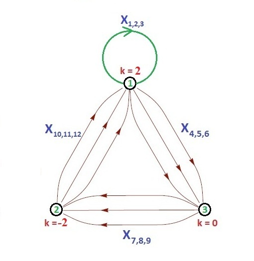
Figure 6: Cyclic quiver for Fano ${\cal B}_{2}$

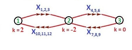
Figure 7: Linear quiver for Fano ${\cal B}_{2}$

Using $W$ given in eqn.(5.1), one can construct $K$ which gives $T$ whence $P$:

$$P=\left(\begin{array}[]{c|cccccccc}&p_{1}&p_{2}&p_{3}&p_{4}&p_{5}&p_{6}&p_{7}&p_{8}\\ \hline\cr X_{1}&2&0&0&2&2&0&0&1\\ X_{2}&0&2&0&2&2&0&0&1\\ X_{3}&0&0&2&2&2&0&0&1\\ X_{4}&2&0&0&0&2&2&0&1\\ X_{5}&0&2&0&0&2&2&0&1\\ X_{6}&0&0&2&0&2&2&0&1\\ X_{7}&4&0&0&2&0&0&2&1\\ X_{8}&0&4&0&2&0&0&2&1\\ X_{9}&0&0&4&2&0&0&2&1\\ X_{10}&4&0&0&0&0&2&2&1\\ X_{11}&0&4&0&0&0&2&2&1\\ X_{12}&0&0&4&0&0&2&2&1\end{array}\right)~{}.$$ (5.2)

A possible choice of the total charge matrix $Q$ is given by:

$$Q=\left(\begin{array}[]{c}Q_{F}\\ \hline\cr Q_{D}\end{array}\right)=\left(\begin{array}[]{cccccccc}1&1&1&-1&-1&-1&-2&2\\ 0&0&0&1&-1&1&-1&0\\ 0&0&0&0&1&0&1&-2\\ \hline\cr 0&0&0&1&1&2&0&-4\end{array}\right)~{}.$$ (5.3)

The toric data of the theory is given as[23]:

$${\cal{G}}(2,-2,0)=\left(\begin{array}[]{cccccccc}p_{1}&p_{2}&p_{3}&p_{4}&p_{5}&p_{6}&p_{7}&p_{8}\\ \hline\cr 1&1&1&1&1&1&1&1\\ 1&-1&0&0&0&0&0&0\\ 0&1&-1&0&0&0&0&0\\ 0&0&1&-1&-1&1&1&0\end{array}\right)~{}.$$ (5.4)

Taking the $P$ matrix (5.2), giving VEV to any of the matter fields gives ${Q_{F}}_{r}=0$. Also from coalescing of nodes in the quiver diagrams given in figure 6 and figure 7, we know that the non-trivial CS level of the 2 node daughter theory will be $(2,-2)$. Thus, the daughter theory will be $\mbox{$\mathbb{Z}$}_{2}$ orbifolds of $\mbox{$\mathbb{C}$}^{4}$. From eqn.(5.2) we see that giving a VEV to any of the matter fields will always remove the last column ($p_{8}$) of the $P$ which corresponds to an internal point in the toric diagram of ${\cal B}_{2}$. So if we do the algebraic higgsing of ${\cal B}_{2}$, we are never going to get the embedding as Fano $\mbox{$\mathbb{P}$}^{3}$ which has an internal point in its toric diagram. We will now work out the partial resolution to see if we can get more information.

5.1 Partial Resolution

In this case, we found that the if we remove the set of points $\left\{p_{1},p_{4},p_{5},p_{7}\right\}$, $\left\{p_{1},p_{4},p_{6},p_{7}\right\}$, $\left\{p_{2},p_{4},p_{5},p_{7}\right\}$, $\left\{p_{2},p_{4},p_{6},p_{7}\right\}$, $\left\{p_{3},p_{4},p_{5},p_{7}\right\}$, $\left\{p_{3},p_{4},p_{6},p_{7}\right\}$ or $\left\{p_{4},p_{5},p_{6},p_{7}\right\}$, we will get a reduced toric data which is related to ${\cal{G}}_{a}(k=1)$ or ${\cal{G}}_{b}(k=1)$ by a $GL(4,\mbox{$\mathbb{Z}$})$ transformation. Further the nullspace, i.e. the reduced charge matrix $Q_{r}$ is trivial. This implies that the toric data of the daughter theory is $\mbox{$\mathbb{C}$}^{4}$.

5.1.1 Embedding of Fano $\mbox{$\mathbb{P}$}^{3}$ inside Fano ${\cal B}_{2}$

If we remove the points $\left\{p_{5},p_{6},p_{7}\right\}$ from the toric data ${\cal{G}}$ given in eqn.(5.4), we will get the reduced toric data:

$${\cal{G}}_{r}=\left(\begin{array}[]{ccccc}p_{1}&p_{2}&p_{3}&p_{4}&p_{8}\\ \hline\cr 1&1&1&1&1\\ 1&-1&0&0&0\\ 0&1&-1&0&0\\ 0&0&1&-1&0\end{array}\right)~{},$$

which is exactly same as the toric data of $\mbox{$\mathbb{P}$}^{3}$. Thus we see that $\mbox{$\mathbb{P}$}^{3}$ is embedded inside ${\cal B}_{2}$.

Taking a row ($r$) of total charge $Q$ of the daughter theory as a linear combination of rows ($R_{i}$) of total charge matrix of ${\cal B}_{2}$ given in eqn.(5.3):

$$r=(a_{1},a_{1},a_{1},-a_{1}+a_{2}+a_{4},-a_{1}-a_{2}+a_{3}+a_{4},-a_{1}+a_{2}+2a_{4},-2a_{1}-a_{2}+a_{3},2a_{1}-2a_{3}-4a_{4})~{}.$$

Setting the columns 5,6,7 in $r$ to 0, we get $a_{1}=a_{2}/3=a_{3}/5=-a_{4}$. The reduced charge matrix after removal of the columns 5,6,7 gives:

$$r=(a_{1},a_{1},a_{1},a_{1},-4a_{1})=a_{1}(1,1,1,1,-4)~{}.$$

Thus, $Q$ will have only 1 row generated by $(1,1,1,1,-4)$. Hence, the charge matrix of daughter theory is $Q=(Q_{F})=(1,1,1,1,-4)$ which is the charge matrix of $\mbox{$\mathbb{P}$}^{3}$. Thus partial resolution only gives $\mbox{$\mathbb{P}$}^{3}$. However from coalescing of nodes in figures 6 and 7, we expect the daughter theory to be $\mbox{$\mathbb{Z}$}_{2}$ orbifold of $\mbox{$\mathbb{P}$}^{3}$.

6 Fano ${\cal B}_{1}$

This theory was studied in [23] where the inverse algorithm was used to find a quiver gauge theory shown in figure 8 with CS levels ($2,0,-2$). The superpotential of this theory was obtained as:

$$W=\text{Tr}\left[X_{2}X_{5}X_{8}\left(X_{1}X_{4}X_{9}X_{3}X_{6}X_{7}-X_{1}X_{6}X_{7}X_{3}X_{4}X_{9}\right)\right]~{}.$$ (6.1)

Note that the abelian $W=0$ and the quiver does not admit tiling. So, there is no way to obtain the toric data of this theory using forward algorithm or dimer tiling approach. The toric data for ${\cal B}_{1}$ theory with multiplicity is given as [23]:

$${\cal{G}}=\left(\begin{array}[]{ccccccc}p_{1}&p_{2}&p_{3}&p_{4}&p_{5}&p_{6}&p_{7}\\ \hline\cr 1&1&1&1&1&1&1\\ 1&-1&0&0&0&0&0\\ 0&1&-1&0&0&0&0\\ 0&0&2&-1&1&1&0\end{array}\right)~{}.$$ (6.2)

From the ansatz given in [23], we can take a choice of $Q_{F}$ and $Q_{D}$ obeying the symmetry of Calabi-Yau over Fano ${\cal B}_{1}$ and the total charge matrix will be given by:

$$Q=\left(\begin{array}[]{c}Q_{F}\\ \hline\cr Q_{D}\end{array}\right)=\left(\begin{array}[]{ccccccc}1&1&1&-2&-2&-2&3\\ 0&0&0&2&1&1&-4\\ \hline\cr 0&0&0&1&0&1&-2\end{array}\right)~{}.$$ (6.3)

The algebraic higgsing in this case gives $\mbox{$\mathbb{Z}$}_{2}$ orbifolds of $\mbox{$\mathbb{C}$}^{4}$ and we also observe that the internal point in the toric Fano ${\cal B}_{1}$ gets removed. The partial resolution by removing the points $\left\{p_{1},p_{4},p_{5}\right\}$, $\left\{p_{2},p_{4},p_{5}\right\}$ or $\left\{p_{3},p_{4},p_{5}\right\}$ gives toric data of $\mbox{$\mathbb{C}$}^{4}$. We could not obtain $\mbox{$\mathbb{P}$}^{3}$ as embedding inside ${\cal B}_{1}$ by this method.

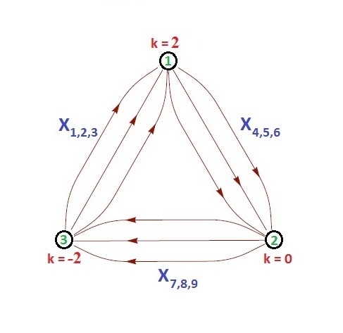
Figure 8: Quiver Diagram for Fano ${\cal B}_{1}$

7 Conclusions

Our main motivation was to determine the $2$-node daughter quivers by the method of higgsing the $3$-node parent quivers. Particularly, we wanted to higgsise matter fields of the $3$-node quivers corresponding to Fano ${\cal B}_{1},{\cal B}_{2},{\cal B}_{3},{\cal B}_{4}$ 3-folds and obtain the daughter quivers. This procedure will determine the CS levels of the daughter quiver theories. Unfortunately, the algebraic method of higgsing does not give any non-trivial charge matrix $Q$.

For the quiver corresponding to Fano ${\cal B}_{4}$, which has dimer tiling presentation, higgsing could be studied by tiling approach as well as by algebraic method. By the algebraic method of higgsing, we get the reduced charge matrix $Q_{r}=0$ which suggests that the two-node daughter theories can be ${\mbox{$\mathbb{C}$}}^{4}$ and orbifolds of ${\mbox{$\mathbb{C}$}}^{4}$. From the method of partial resolution of the toric data corresponding to Fano ${\cal B}_{4}$, we obtained only $\mbox{$\mathbb{C}$}^{4}$. We have shown that the scaling of CS levels $(1,-2,1)\rightarrow(n,-2n,n)$ results in ${\mbox{$\mathbb{Z}$}}_{n}$ orbifolding of Fano ${\cal B}_{4}$ theory. Hence , partial resolution of the orbifolded Fano ${\cal B}_{4}$ will give $\mbox{$\mathbb{C}$}^{4}/\mbox{$\mathbb{Z}$}_{n}$ toric data with trivial $Q_{F}$.

The $3$-node quivers for other Fano ${\cal B}$ which were determined from the inverse algorithm do not admit dimer tiling presentation. So, we cannot study higgsing of these theories from tiling approach. The algebraic higgsing of any matter field removes the information of the internal point in the toric data and always gives trivial reduced charge matrix $Q_{r}=0$. Unlike ${\mbox{$\mathbb{C}$}}^{4}$ and its orbifolds, the toric data of Fano ${\mbox{$\mathbb{P}$}}^{3}$ has an internal point. So, we studied the method of partial resolution for toric Fano ${\cal B}_{1},{\cal B}_{2},{\cal B}_{3}$ 3-folds. We found that the Fano ${\mbox{$\mathbb{P}$}}^{3}$ can be embedded inside Fano ${\cal B}_{3}$ and ${\cal B}_{2}$ theories.

Algebraic higgsing and unhiggsing of quiver theories corresponding to some Fano $3$-folds have been studied recently[25]. Higgsing certain matter fields in the $4$-node quivers corresponding to toric Fano ${\cal C}_{4}$ gives the $3$-node quiver corresponding to Fano ${\cal B}_{4}$. Also higgsing of the quiver corresponding to Fano ${\cal D}_{2}$ gives daughter quiver corresponding to Fano ${\cal B}_{4}$. These results can also be reproduced using the method of partial resolution.

It is not obvious whether we can obtain other Fano ${\cal B}$’s toric data as embeddings inside Fano ${\cal C}_{4}$ and Fano ${\cal D}_{2}$ $3$-folds. One of the issues is about our choice of multiplicity of certain points in the toric data for Fano ${\cal B}_{1},{\cal B}_{2},{\cal B}_{3}$.

We had chosen a charge matrix $Q_{F},Q_{D}$ respecting the ansatz[23] which determined the multiplicity of certain points in the toric data of Fano ${\cal B}$’s. The toric data with the specific multiplicity of certain points was important to obtain sensible quivers. In principle, we would like to do the method of partial resolution for toric data corresponding to some $4$-node quivers and reproduce the toric data of Fano ${\cal B}_{1},{\cal B}_{2},{\cal B}_{3}$ with the correct multiplicity of some of the points. We hope to study in future the embeddings of the toric Fano ${\cal B}$’s inside toric four-folds corresponding to $4$-node quiver Chern-Simons theories.

Acknowledgments: We would like to thank A.Hanany for discussions. We are grateful to T.Sarkar and Rak-Kyeong for their valuable inputs on the orbifolding issues.

References

- [1] J.Bagger and N.Lambert, “Modeling multiple M2’s,” Phys. Rev. D75, 045020 (2007) [arXiv:hep-th/0611108].
- [2] J.Bagger and N.Lambert, “Gauge symmetry and Supersymmetry of Multiple M2-Branes,” Phys. Rev. D77,065008 (2008) [arXiv:0711.0955[hep-th]].
- [3] J.Bagger and N.Lambert, “Comments on Multiple M2-branes,” JHEP0802, 105 (2008) [arXiv:0712.3738[hep-th]].
- [4] A.Gustavsson, “Algebraic structures on parallel M2-branes,” Nucl.Phys. B811, 66 (2009) [arXiv:0709.1260[hep-th]].
- [5] A.Gustavsson,“Selfdual strings and loop space Nahm equations,” JHEP 0804, 083 (2008) [arXiv:0802.3456[hep-th]].
- [6] M.Van Raamsdonk, “Comments on the Bagger-Lambert theory and multiple M2-branes,” JHEP 0805, 105 (2008) [arXiv:0803.3803].
- [7] O.Aharony, O. Bergman, D.L. Jafferis and J. Maldacena, “N=6 superconformal Chern-Simons-matter theories, M2-branes and their gravity duals, ”JHEP 0810,091 (2008) [arXiv:0806.1218[hep-th]].
- [8] I.R.Klebanov and G.Torri, “M2-branes and AdS/CFT,” Int.J.Mod.Phys. A25 332 (2010) [arXiv:0909.1580[hep-th]].
- [9] D.Martelli and J. Sparks, “Moduli spaces of Chern-Simons quiver gauge theories and AdS4/CFT3,” Phys.Rev. D78, 126005 (2008) [arXiv:0808.0912[hep-th]].
- [10] B.Feng, A.Hanany and Y.H.He, “D-brane gauge theories from toric singularities and toric duality,” Nucl. Phys. B595, 165 (2001) [arXiv:hep-th/0003085].
- [11] A. Hanany and K.D. Kennaway, “Dimer models and toric diagrams,” [arXiv:hep-th/0503149].
- [12] S.Franco, A.Hanany, K.D. Kennaway,D.Vegh and B.Wecht, “Brane dimers and quiver gauge theories,” JHEP 0601, 096 (2006) [arXiv:hep-th/ 0504110].
- [13] A.Hanany and A.Zaffaroni, “Tilings, Chern-Simons Theories and M2 branes,” JHEP 0810, 111 (2008) [arXiv:0808.1244[hep-th]].
- [14] K.Ueda and M.Yamazaki, “Toric Calabi-Yau four-folds dual to Chern-Simons-matter theories,” JHEP 0812, 045 (2008) [arXiv:0808.3768[hep-th]].
- [15] A.Hanany, D.Vegh, A.Zaffaroni, “Brane Tilings and M2 branes,” JHEP 0903, 012 (2009) [arXiv:0809.1440].
- [16] S.Franco, A.Hanany, J.Park and D.Rodriguez-Gomez,“Towards M2-brane Theories for Generic Toric Singularities,”JHEP 0812, 110 (2008) [arXiv:0809.3237 [hep-th]].
- [17] A.Hanany and Y.H.He, “M2-branes and Quiver Chern-Simons: A Taxonomic Study,” arXiv:0811.4044[hep-th].
- [18] J.Davey, A.Hanany, N.Mekareeya and G.Torri, “Phases of M2-brane Theories,” JHEP 0906, 025 (2009) [arXiv:0903.3234[hep-th]].
- [19] J.Davey, A.Hanany, N.Mekareeya and G.Torri, “Higgsing M2-brane Theories,” arXiv:0908.4033[hep-th].
- [20] J.Davey, A.Hanany, N.Mekareeya and G.Torri, “M2-Branes and Fano 3-folds,” arXiv:1103.0553[hep-th].
- [21] K. Watanabe, M. Watanabe, Tokyo J. Math, 5, no. 1 (1982)
- [22] V. V. Batyrev, “Toroidal Fano 3-folds,” Math. USSR-Izv 19, 13 (1982)
- [23] S. Dwivedi, P. Ramadevi, “Inverse algorithm and M2-brane theories,” JHEP 1111, 111 (2011) [arXiv:1108.2387v3 [hep-th]].
- [24] P. Agarwal, P. Ramadevi, T. Sarkar, “A note on dimer models and D-brane gauge theories,” JHEP 0806 054 (2008) [arXiv:0804.1902].
- [25] Prabwal Phukon, Tapobrata Sarkar, “On the Higgsing and UnHiggsing of Fano 3-Folds,” JHEP 1201 090 (2012) [arXiv:1108.4237v1].