Collective modes of the order parameter in a triplet superfluid neutron liquid

Abstract

The complete spectrum of collective modes of the triplet order parameter in the superfluid neutron matter is examined in the BCS approximation below the pair-breaking threshold. The dispersion equations both for the unitary and nonunitary excitations are derived and solved in the limit of $q\rightarrow 0$ by taking into account the anisotropy of the energy gap for the case of $P$-wave pairing. By our analysis, there is only one Goldstone mode which is associated with the broken gauge symmetry. We found no additional Goldstone modes associated with the broken rotational symmetry but found that the oscillations of the total angular momentum are qualitatively similar to the ”normal-flapping” mode in the A-phase of superfluid Helium. There are also two collective modes associated with internal vibrations of the structure of the order parameter oscillating with $\omega\left(T=0\right)=1.20\Delta_{0}$ and $\omega\left(T=0\right)=0.61\Delta_{0}$.

LABEL:FirstPage1

I Introduction

The neutron star evolution is governed mostly by microscopic processes occuring in its volume and depend substantially on the spectrum of thermal excitations that can exist in the bulk baryon matter. Strong and electromagnetic interactions form numerous collective excited states in the normal (nonsuperfluid) component of the neutron star matter which have been extensively studied by many authors. H78 -PB .

The purpose of this paper is to present the complete spectrum of collective modes in the superfluid phase of superdense neutron matter. It is generally accepted that the pair condensation in superdense neutron matter occurs into the ${}^{3}P_{2}$ state (with a small admixture of ${}^{3}F_{2}$ ). Such a model is based on the properties of the bare $NN$ interaction, which contains a relatively strong spin-orbit interaction in this channel. Strictly speaking, it is not really clear that a ${}^{3}P_{2}$ pairing instability will survive at the relevant densities in neutron stars (double nuclear saturation density, or more), due to uncertainties in the 3$N$ interaction. Nevertheless this model is conventionally used for estimates of neutrino energy losses in the minimal cooling scenarios of neutron stars.

We do not consider the well discussed processes of pair breaking and formation YKL , L10a but focus on the undamped collective oscillations of the order parameter. The collective excitations below the pair-breaking threshold can play an important role in the thermodynamic properties of the neutron liquid at lowest temperatures when the other possible excitations are strongly suppressed by the superfluidity. Some properties of the anisotropic Goldstone mode in the neutron condensate were discussed in Ref. L11a , and the existence of two spin-wave modes was predicted recently L10b -L11c in the average-angle approximation. In the present paper we consider the solution to the dispersion equations by taking into account the anisotropy of the energy gap and find the whole spectrum of the undamped collective oscillations of the ${}^{3}P_{2}$ order parameter.

In applications to neutron stars it is customary hof to consider the ${}^{3}P_{2}$ state with a preferred magnetic quantum number $M=0$. Sophisticated calculations Khodel -0203046 have shown that, besides the above one-component state, there are also multicomponent states involving several magnetic quantum numbers that compete in energy and represent various phase states of the condensate dependent on the temperature. A delicate difference in the above gap magnitudes occurs owing to small tensor interactions between paired quasiparticles. If we neglect the tensor interactions the multicomponent states are degenerate and can be obtained from the state $M=0$ by trivial rotation of the frame in space. We therefore will focus on the ${}^{3}P_{2}$ neutron pairing into a state with $M=0$.

Previously eigen-modes of the order parameter have been thoroughly studied in the superfluid liquid ³He Wolfe73 -Wolfe1 . The complete analysis of the order-parameter collective modes in anisotropic ³He-A is given in Ref. W . The pairing interaction in ³He is invariant with respect to the rotation of spin and orbital coordinates separately. This admits spin fluctuations independent of the orbital coordinates. In contrast, the spin-triplet neutron condensate arises in the high-density neutron matter mostly owing to the attractive spin-orbit interactions which do not possess the above symmetry. Therefore the results obtained for liquid ³He can not be applied directly to the spin-triplet neutron superfluid, where the most attractive channel of interactions corresponds to spin, orbital, and total angular momenta $S=1$, $L=1$, and $J=2$, respectively, and pairs quasiparticles into the ${}^{3}P_{2}$ states with the projection of the total angular momentum $M=0,\pm 1,\pm 2$.

As is well known the strong interactions in the neutron matter are not restricted by the pairing forces. One can expect that the Fermi-liquid effects are able to renormalize the collective modes. We hope however that the principal effect occurs in the case of the Goldstone mode, where the sound velocity is strongly renormalized by the particle-hole interactions. This effect was already considered in Ref. L11a . Since the Landau parameters are unknown for a dense asymmetric baryon matter it would be meaningless to complicate the calculations by the Fermi liquid effects. Therefore we discard residual particle-hole interactions and consider the problem in the BCS model.

The paper is organized as follows. Section II contains some preliminary notes. We consider the nonequilibrium gap equations for the case of spin-orbit pairing forces and discuss the renormalizations which transform the standard gap equations to a very simple form valid near the Fermi surface. In Sec. III we consider small deviations of the condensate from equilibrium caused by weak external fields and derive the equations for the relevant anomalous three-point vertices. In Sec. IV we derive, in the BCS approximation, the dispersion equations for eigenmodes of the order parameter and find the whole spectrum of the undamped oscillations. Section V represents a discussion of the obtained results and the conclusion. Some intermediate and additional calculations are contained in three appendices for a more deep understanding.

Throughout this paper, we use the standard model of weak interactions, the system of units $\hbar=c=1$ and the Boltzmann constant $k_{B}=1$.

II Formalism

We employ the Matsubara calculation technique for the system in thermal equilibrium and use the standard notation for ordinary propagators of a quasiparticle and a hole, $\hat{G}\left(p_{\kappa}.\mathbf{p}\right)=\parbox{28.45274pt}{\includegraphics[width=28.45274pt]{Gn.eps}}$, $\hat{G}^{-}\left(p_{\kappa}.\mathbf{p}\right)\equiv\hat{G}\left(-p_{\kappa},-\mathbf{p}\right)=\parbox{28.45274pt}{\includegraphics[width=28.45274pt,angle={180}]{Gn.eps}}$, and for anomalous propagators $\hat{F}^{\left(1\right)}=\parbox{28.45274pt}{\includegraphics[width=28.45274pt]{F1.eps}}$ , $\hat{F}^{\left(2\right)}=\parbox{28.45274pt}{\includegraphics[width=28.45274pt]{F2.eps}}$ in the momentum representation, where $\mathbf{p}$ is the quasiparticle momentum, and $p_{\kappa}=\left(2\kappa+1\right)\pi T$ with $\kappa=0,\pm 1,\pm 2,...$ is the fermionic Matsubara frequency which depends on the temperature $T$.

The triplet order parameter, $\hat{D}\equiv D_{\alpha\beta}\left(\mathbf{n}\right)$, in the neutron superfluid represents a symmetric matrix in spin space $\left(\alpha,\beta=\uparrow,\downarrow\right)$ which can be written as $\hat{D}\left(\mathbf{n}\right)=\Delta\mathbf{\bar{b}}\bm{\hat{\sigma}}\hat{g}$, where $\bm{\hat{\sigma}}=\left(\hat{\sigma}_{1},\hat{\sigma}_{2},\hat{\sigma}_{3}\right)$ are Pauli spin matrices, and $\hat{g}=i\hat{\sigma}_{2}$. The angular dependence of the order parameter is represented by Cartesian components of the unit vector $\mathbf{n=p}/p$ which involves the polar angles on the Fermi surface,

$$n_{1}=\sin\theta\ \cos\varphi,\ \ \ n_{2}=\sin\theta\ \sin\varphi,\ \ \ n_{3}=\cos\theta.$$ (1)

The temperature-dependent gap amplitude $\Delta\left(T\right)$ is a real constant (on the Fermi surface), and $\mathbf{\bar{b}}\left(\mathbf{n}\right)$ is a real vector in spin space which we normalize by the condition

$$\left\langle\bar{b}^{2}\left(\mathbf{n}\right)\right\rangle=1~{}.$$ (2)

Hereafter we use the angle brackets to denote angle averages,

$$\left\langle...\right\rangle\equiv\frac{1}{4\pi}\int d\mathbf{n}\cdot\cdot\cdot=\frac{1}{2}\int_{-1}^{1}dn_{3}\int_{0}^{2\pi}\frac{d\varphi}{2\pi}\cdot\cdot\cdot.$$ (3)

The analytic form of the quasiparticle propagators can be written as

$$\hat{G}\left(p_{\kappa},\mathbf{p}\right)=G\left(p_{\kappa},\mathbf{p}\right)\hat{1},~{}\ \ \hat{F}^{\left(1\right)}=F\left(p_{\kappa},\mathbf{p}\right)\mathbf{\bar{b}}\hat{\bm{\sigma}}\hat{g},$$ (4)

$$\ \hat{F}^{\left(2\right)}=\hat{F}^{+}\left(-p_{\kappa},-\mathbf{p}\right)=\hat{g}\hat{\bm{\sigma}}\mathbf{\bar{b}}F\left(p_{\kappa},\mathbf{p}\right),$$ (5)

where we define the scalar Green functions

$$G\left(p_{\kappa},\mathbf{p}\right)=\frac{-ip_{\kappa}-\varepsilon_{p}}{p_{\kappa}^{2}+E_{\mathbf{p}}^{2}},~{}\ \ F\left(p_{\kappa},\mathbf{p}\right)=\frac{\Delta}{p_{\kappa}^{2}+E_{\mathbf{p}}^{2}}.$$ (6)

The quasiparticle energy is given by

$$E_{\mathbf{p}}=\sqrt{\varepsilon_{p}^{2}+\Delta^{2}\bar{b}^{2}\left(\mathbf{n}\right)}$$ (7)

with

$$\varepsilon_{p}\simeq\upsilon_{F}\left(p-p_{F}\right),$$ (8)

where $\upsilon_{F}\ll 1$ is the Fermi velocity of the nonrelativistic neutrons.

At equilibrium, the gap matrix $\hat{D}$ is connected to the anomalous Green’s function $\hat{F}$ by the gap equation gapEq

$$D_{\alpha\beta}\left(\mathbf{p}\right)=-T\sum_{\kappa}\int\frac{d^{3}p^{\prime}}{8\pi^{3}}\Gamma_{\alpha\gamma,\beta\delta}\left(\mathbf{p,p}^{\prime}\right)F_{\gamma\delta}\left(p_{\kappa}.\mathbf{p}^{\prime}\right),$$ (9)

where $\Gamma_{\alpha\beta,\gamma\delta}\left(\mathbf{p,p}^{\prime}\right)$ stands for the block of the interaction diagrams irreducible in the channel of two quasiparticles.

We consider small periodic departure from equilibrium of the form $\propto\exp\left(i\mathbf{qr}-i\omega t\right)$. By assuming that the interactions between quasiparticles are essentially instantaneous on the time scale of the oscillation frequencies the nonequilibrium (time-dependent) gap matrices $\mathfrak{D}_{\alpha\beta}\left(\omega\mathbf{,q;p}\right)\exp\left(i\mathbf{qr}-i\omega t\right)$ must obey the self-consistency conditions (gap equations) which depend now on the energy $\omega$ and space momentum $\mathbf{q}$ of the perturbation. Then the order parameters $\mathfrak{D}_{\alpha\beta}^{\left(1,2\right)}\left(\omega\mathbf{,q;p}\right)$ are to be found as the analytic continuation of the functions $\mathfrak{D}_{\alpha\beta}^{\left(1,2\right)}\left(\omega_{\eta}\mathbf{,q;p}\right)$ connected to the anomalous Green functions $\mathcal{\hat{F}}_{\gamma\delta}^{\left(1,2\right)}\left(\omega_{\eta}\mathbf{,q};p_{\kappa}\mathbf{,p}\right)$ by the equations

$$\mathfrak{D}_{\alpha\beta}^{\left(1\right)}\left(\omega_{\eta}\mathbf{,q;p}\right)=-T\sum_{\kappa}\int\frac{d^{3}p^{\prime}}{8\pi^{3}}\Gamma_{\alpha\gamma,\beta\delta}\left(\mathbf{p,p}^{\prime}\right)\mathcal{\hat{F}}_{\gamma\delta}^{\left(1\right)}\left(\omega_{\eta}\mathbf{,q;}p_{\kappa},\mathbf{p}^{\prime}\right),$$ (10)

$$\mathfrak{D}_{\alpha\beta}^{\left(2\right)}\left(\omega_{\eta}\mathbf{,q;p}\right)=-T\sum_{\kappa}\int\frac{d^{3}p^{\prime}}{8\pi^{3}}\Gamma_{\beta\delta,\alpha\gamma}\left(\mathbf{p}^{\prime}\mathbf{,p}\right)\mathcal{\hat{F}}_{\gamma\delta}^{\left(2\right)}\left(\omega_{\eta}\mathbf{,q;}p_{\kappa},\mathbf{p}^{\prime}\right),$$ (11)

where $\omega_{\eta}=2i\pi\eta T$ with $\eta=0,\pm 1,\pm 2,...$ is the bosonic Matsubara frequency.

In these equations, the integration goes over infinite momentum space while the quasiparticle approach is valid only near the Fermi surface. To get rid of the integration over the regions far from the Fermi surface in Eqs. (10) and (11), we renormalize the interaction as suggested in Refs. Larkin , Leggett . We define

$$\Gamma_{\alpha\gamma,\beta\delta}^{r}\left(\mathbf{p,p}^{\prime};T\right) =\Gamma_{\alpha\gamma,\beta\delta}\left(\mathbf{p,p}^{\prime}\right)$$

$$-T\sum_{\kappa}\int\frac{dp^{\prime\prime}p^{\prime\prime 2}}{\pi^{2}\varrho}\Gamma_{\alpha\mu,\beta\nu}\left(\mathbf{p,p}^{\prime\prime}\right)\left(GG^{-}\right)_{N}^{\prime\prime}\Gamma_{\mu\gamma,\nu\delta}^{r}\left(\mathbf{p}^{\prime\prime}\mathbf{,p}^{\prime};T\right),$$ (12)

where $\varrho=p_{F}M^{\ast}/\pi^{2}$, the effective mass of a neutron quasiparticle is defined as $M^{\ast}=p_{F}/\upsilon_{F}$, and the product $\left(GG^{-}\right)_{N}^{\prime\prime}\equiv G_{N}\left(p_{\kappa},\mathbf{p}^{\prime\prime}\right)G_{N}\left(-p_{\kappa},-\mathbf{p}^{\prime\prime}\right)$ is evaluated in the normal (nonsuperfluid) state by assuming $G_{N}\left(p_{\kappa},\mathbf{p}\right)=\left(ip_{\kappa}-\varepsilon_{p}\right)^{-1}$.

By acting from the left onto the both sides of Eqs. (10) and (11) by the operator

$$1-T\sum_{\kappa}\int\frac{dp^{\prime\prime}p^{\prime\prime 2}}{\pi^{2}\varrho}\Gamma_{\alpha\mu,\beta\nu}^{r}\left(\mathbf{p,p}^{\prime\prime};T\right)\left(GG^{-}\right)_{N}^{\prime\prime}\cdot\cdot\cdot,$$ (13)

and making use of the fact that

$$\Gamma_{\alpha\gamma,\beta\delta}^{r}\left(\mathbf{p,p}^{\prime};T\right) =\Gamma_{\alpha\gamma,\beta\delta}\left(\mathbf{p,p}^{\prime}\right)$$

$$-T\sum_{\kappa}\int\frac{dp^{\prime\prime}p^{\prime\prime 2}}{\pi^{2}\varrho}\Gamma_{\alpha\mu,\beta\nu}^{r}\left(\mathbf{p,p}^{\prime\prime};T\right)\left(GG^{-}\right)_{N}^{\prime\prime}\Gamma_{\mu\gamma,\nu\delta}\left(\mathbf{p}^{\prime\prime}\mathbf{,p}^{\prime}\right),$$ (14)

we can recast Eqs. (10) and (11) to the form

$$\mathfrak{D}_{\alpha\beta}^{\left(1\right)}\left(\mathbf{p}\right)=-T\sum_{\kappa}\int\frac{d^{3}p^{\prime}}{8\pi^{3}}\Gamma_{\alpha\gamma,\beta\delta}^{r}\left(\mathbf{p,p}^{\prime}\right)\left[\mathcal{\hat{F}}_{\gamma\delta}^{\left(1\right)}-\mathfrak{D}_{\gamma\delta}^{\left(1\right)}G_{N}G_{N}^{-}\right]_{\mathbf{p}^{\prime}},$$ (15)

$$\mathfrak{D}_{\alpha\beta}^{\left(2\right)}\left(\mathbf{p}\right)=-T\sum_{\kappa}\int\frac{d^{3}p^{\prime}}{8\pi^{3}}\Gamma_{\beta\delta,\alpha\gamma}^{r}\left(\mathbf{p}^{\prime}\mathbf{,p}\right)\left[\mathcal{\hat{F}}_{\gamma\delta}^{\left(2\right)}-\mathfrak{D}_{\gamma\delta}^{\left(2\right)}G_{N}G_{N}^{-}\right]_{\mathbf{p}^{\prime}}.$$ (16)

For brevity we omit the dependence of functions on $\omega_{\eta}$ and $\mathbf{q}$. The product $G_{N}G_{N}^{-}$ is to be evaluated for $\omega_{\eta}=0$, $\mathbf{q}=0$. In these equations the integrand decreases very rapidly with the distance from the Fermi surface. Since we are interested in the processes near the Fermi surface, we can replace all smooth functions of the momentum $p$ with their expressions at $p=p_{F}$.

The pairing in the high-density neutron matter is mostly caused by the attractive spin-orbit interactions. In the vector notation one can write the renormalized ${}^{3}P_{2}$ interaction in the form

$$\varrho\Gamma_{\alpha\gamma,\beta\delta}^{r}\left(\mathbf{p,p}^{\prime}\right)=-V\sum_{M=-2}^{2}\left[\mathbf{b}_{M}(\mathbf{n})\cdot\hat{\bm{\sigma}}\hat{g}\right]_{\alpha\beta}\left[\hat{g}\hat{\bm{\sigma}}\cdot\mathbf{b}_{M}^{\ast}(\mathbf{n}^{\prime})\right]_{\gamma\delta}~{},$$ (17)

where $V$ is the constant amplitude taken at the Fermi surface, and $\mathbf{b}_{M}\left(\mathbf{n}\right)$ are the vectors in spin space which generate standard spin-angle matrices according to

$$\frac{1}{\sqrt{8\pi}}\mathbf{b}_{M}(\mathbf{n})\bm{\hat{\sigma}}\hat{g}\equiv\sum_{M_{S}+M_{L}=M}\left(\frac{1}{2}\frac{1}{2}\alpha\beta|1M_{S}\right)\left(11M_{S}M_{L}|2M\right)Y_{1,M_{L}}\left(\mathbf{n}\right).$$ (18)

These are given by

$$\mathbf{b}_{0} =\sqrt{1/2}\left(-n_{1},-n_{2},2n_{3}\right),\mathbf{b}_{1}=-\sqrt{3/4}\left(n_{3},in_{3},n_{1}+in_{2}\right),$$

$$\mathbf{b}_{2} =\sqrt{3/4}\left(n_{1}+in_{2},in_{1}-n_{2},0\right),\mathbf{b}_{-M}=\left(-\right)^{M}\mathbf{b}_{M}^{\ast}.$$ (19)

The vectors are mutually orthogonal and are normalized by the condition

$$\left\langle\mathbf{b}_{M^{\prime}}^{\ast}\mathbf{b}_{M}\right\rangle=\delta_{M^{\prime}M}.$$ (20)

It is convenient to divide the integration over the momentum space into integration over the solid angle and over the energy according to

$$\int\frac{d^{3}p}{\left(2\pi\right)^{3}}\operatorname*{Tr}\left(...\right)=\varrho\int\frac{d\mathbf{n}}{4\pi}\int_{-\infty}^{\infty}d\varepsilon_{p}\frac{1}{2}\operatorname*{Tr}\left[...\right]\cdot\cdot\cdot,$$ (21)

and denote

$$\sum_{p,\kappa}...\equiv\int_{-\infty}^{\infty}d\varepsilon_{p}T\sum_{\kappa}\cdot\cdot\cdot.$$

Then instead of Eqs. (15) and (16) we obtain

$$\mathfrak{\hat{D}}^{\left(1\right)}\left(\mathbf{n}\right) =V\sum_{M}\mathbf{b}_{M}\hat{\left(\mathbf{n}\right)\bm{\sigma}}\hat{g}$$

$$\times\left\langle\sum_{p,\kappa}\frac{1}{2}\operatorname*{Tr}\left[\hat{g}\left(\hat{\bm{\sigma}}\mathbf{b}_{M}^{\ast}\right)\left(\mathcal{\hat{F}}^{\left(1\right)}-\mathfrak{\hat{D}}^{\left(1\right)}G_{N}G_{N}^{-}\right)\right]\right\rangle_{\mathbf{n}^{\prime}},$$ (22)

$$\mathfrak{\hat{D}}^{\left(2\right)}\left(\mathbf{n}\right) =V\sum_{M}\hat{g}\hat{\bm{\sigma}}\mathbf{b}_{M}\left(\mathbf{n}\right)$$

$$\times\left\langle\sum_{p,\kappa}\frac{1}{2}\operatorname*{Tr}\left[\left(\mathbf{b}_{M}^{\ast}\hat{\bm{\sigma}}\right)\hat{g}\left(\mathcal{\hat{F}}^{\left(2\right)}-\mathfrak{\hat{D}}^{\left(2\right)}G_{N}G_{N}^{-}\right)\right]\right\rangle_{\mathbf{n}^{\prime}},$$ (23)

where the dependence of functions on $\omega_{\eta}$ and $\mathbf{q}$ is again omitted.

In the absence of external fields the equilibrium order parameters are of the simple form

$$\hat{D}^{\left(1\right)}\left(\mathbf{n}\right)=\hat{D}\left(\mathbf{n}\right)=\Delta\mathbf{\bar{b}}\bm{\sigma}\hat{g},$$ (24)

$$\hat{D}^{\left(2\right)}\left(\mathbf{n}\right)=\hat{D}^{+}\left(-\mathbf{n}\right)=\Delta\hat{g}\hat{\bm{\sigma}}\mathbf{\bar{b}}.$$ (25)

From Eqs. (22) and (23) we obtain

$$\Delta\mathbf{\bar{b}}\left(\mathbf{n}\right)=V\sum_{M}\mathbf{b}_{M}\left(\mathbf{n}\right)\left\langle\mathbf{b}_{M}^{\ast}\mathbf{\bar{b}}\sum_{p,\kappa}\left(F-\Delta G_{N}G_{N}^{-}\right)\right\rangle_{\mathbf{n}^{\prime}}.$$ (26)

Using also the fact that $F\equiv\Delta\left(GG^{-}+\bar{b}^{2}FF\right)$, Eq. (26) can be written in the form

$$\mathbf{\bar{b}}\left(\mathbf{n}\right)=V\sum_{M}\mathbf{b}_{M}(\mathbf{n})\left\langle\mathbf{\bar{b}b}_{M}^{\ast}A\right\rangle,$$ (27)

where the function $A$ is defined as

$$A\left(\mathbf{n}\right)=\int_{-\infty}^{\infty}d\varepsilon_{p}T\sum_{\kappa}\left(GG^{-}-G_{N}G_{N}^{-}+\bar{b}^{2}FF\right).$$ (28)

Its explicit form is given in Eq. (43).

With the aid of the expansion

$$\mathbf{\bar{b}}\left(\mathbf{n}\right)=\sum_{M}\left\langle\mathbf{\bar{b}b}_{M}^{\ast}\right\rangle\mathbf{b}_{M}(\mathbf{n}),$$ (29)

and of Eqs. (2) and (20) one can recast Eq. (27) as

$$1=V\left\langle\bar{b}^{2}A\right\rangle.$$ (30)

III Vertex equations

We now consider the order parameter of the superfluid Fermi-liquid in weak external fields $A^{\mu}\left(\omega,\mathbf{q}\right)\exp\left(i\mathbf{qr}-i\omega t\right)$. The field interaction with a superfluid should be described with the aid of four effective three-point vertices. There are two ordinary effective vertices, $\hat{\tau}_{\mu}\left(\omega,\mathbf{q;p}\right)$ and $\hat{\tau}_{\mu}^{-}\left(\mathbf{p}\right)=\hat{\tau}_{\mu}^{T}\left(-\mathbf{p}\right)$, corresponding to the creation of a particle and a hole by the field (These differ by direction of fermion lines), and two anomalous vertices $\hat{T}_{\mu}^{\left(1,2\right)}\left(\omega,\mathbf{q;p}\right)$ corresponding to the creation of two particles or two holes. The latter describe the linear departure from equilibrium of the matrix order parameters caused by the external field of wave vector $\mathbf{q}$ and frequency $\omega$:

$$\delta\hat{D}^{\left(1,2\right)}\left(\omega\mathbf{,q;p}\right)=e\hat{T}_{\mu}^{\left(1,2\right)}\left(\omega,\mathbf{q;p}\right)A^{\mu}\left(\omega,\mathbf{q}\right).$$ (31)

Here the coupling constant $e$ is specified by the external field and a summation over repeated Dirac indices $\mu=0,1,2,3$ is implied. The linearization of Eqs. (22) and (23) by taking into account Eq. (26) results in equations for the anomalous three-point vertices $\hat{T}_{\mu}^{\left(1,2\right)}(\omega\mathbf{,q;n})$

$$\hat{T}_{\mu}^{\left(1\right)} =-V\sum_{M}\mathbf{b}_{M}\hat{\bm{\sigma}}\hat{g}$$

$$\times\left\langle\sum_{p,\kappa}\frac{1}{2}\operatorname*{Tr}\left[\hat{g}\hat{\bm{\sigma}}\mathbf{b}_{M}^{\ast}\left(\frac{\delta\mathcal{\hat{F}}^{\left(1\right)}}{eA^{\mu}}-\hat{T}_{\mu}^{\left(1\right)}G_{N}G_{N}^{-}\right)\right]\right\rangle,$$ (32)

$$\hat{T}_{\mu}^{\left(2\right)} =-V\sum_{M}\hat{g}\hat{\bm{\sigma}}~{}\mathbf{b}_{M}$$

$$\times\left\langle\sum_{p,\kappa}\frac{1}{2}\operatorname*{Tr}\left[\mathbf{b}_{M}^{\ast}\hat{\bm{\sigma}}\hat{g}\left(\frac{\delta\mathcal{\hat{F}}^{\left(2\right)}}{eA^{\mu}}-\hat{T}_{\mu}^{\left(2\right)}G_{N}G_{N}^{-}\right)\right]\right\rangle,$$ (33)

where the product $G_{N}G_{N}^{-}$ is to be evaluated for $\omega=0,\mathbf{q}=0$. The corrections to the anomalous propagators $\delta\mathcal{\hat{F}}^{\left(1,2\right)}$ arise owing to the variation of the order parameters and the ordinary self-energy of a quasiparticle in the external field and can be depicted symbolically by the graphs in Fig. 1.

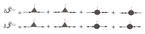
Figure 1: Graphs corresponding to linear corrections to the anomalous propagators. The external field is shown by dashed lines. The anomalous vertices are shown by filled triangles. Filled circles are dressed ordinary vertices.

Analytically one has

$$\frac{\delta\mathcal{\hat{F}}^{\left(1\right)}}{eA^{\mu}} \simeq\hat{G}\left(P_{+}\right)\hat{T}_{\mu}^{\left(1\right)}\hat{G}^{-}\left(P_{-}\right)+\hat{F}^{\left(1\right)}\left(P_{+}\right)\hat{T}_{\mu}^{\left(2\right)}\hat{F}^{\left(1\right)}\left(P_{-}\right)$$

$$+\hat{G}\left(P_{+}\right)\hat{\tau}_{\mu}\hat{F}^{\left(1\right)}\left(P_{-}\right)+\hat{F}^{\left(1\right)}\left(P_{+}\right)\hat{\tau}_{\mu}^{-}\hat{G}^{-}\left(P_{-}\right),$$ (34)

and

$$\frac{\delta\mathcal{\hat{F}}^{\left(2\right)}}{eA^{\mu}} \simeq\hat{G}^{-}\left(P_{+}\right)\hat{T}_{\mu}^{\left(2\right)}\hat{G}\left(P_{-}\right)+\hat{F}^{\left(2\right)}\left(P_{+}\right)\hat{T}_{\mu}^{\left(1\right)}\hat{F}^{\left(2\right)}\left(P_{-}\right)$$

$$+\hat{F}^{\left(2\right)}\left(P_{+}\right)\hat{\tau}_{\mu}\hat{G}\left(P_{-}\right)+\hat{G}^{-}\left(P_{+}\right)\hat{\tau}_{\mu}^{-}\hat{F}^{\left(2\right)}\left(P_{-}\right),$$ (35)

where we denote $P_{+}=\left\{p_{\kappa}+\omega_{\eta},\mathbf{p}+\frac{1}{2}\mathbf{q}\right\}$ and $P_{-}=\left\{p_{\kappa},\mathbf{p}-\frac{1}{2}\mathbf{q}\right\}$.

We shall examine collective excitations of the condensate below the pair-breaking threshold. The eigenmodes are known to manifest themselves as sharp resonances of the linear response of the medium onto external perturbations. Throughout this paper we consider the case of ${}^{3}P_{2}$ neutron pairing, when quasiparticles pair in the most attractive channel with spin, orbital and total angular momenta, $S=1,L=1,J=2$, respectively. This allows one to search for the anomalous vertices near the Fermi surface in the form of expansions over the eigen functions of the total angular momentum $(J,M)$ with $J=2$ and $M=0,\pm 1,\pm 2$:

$$\hat{T}^{\left(1\right)}\left(\omega,\mathbf{q;n}\right)=\sum_{M}B_{M}^{\left(1\right)}\left(\omega,\mathbf{q}\right)\left(\bm{\hat{\sigma}}\mathbf{b}_{M}\right)\hat{g},$$ (36)

$$\hat{T}^{\left(2\right)}\left(\omega,\mathbf{q;n}\right)=\sum_{M}B_{M}^{\left(2\right)}\left(\omega,\mathbf{q}\right)\hat{g}\left(\bm{\hat{\sigma}}\mathbf{b}_{M}\right).$$ (37)

Hereafter we omit the Dirac indices by assuming that the equations are valid for each of the vertex components. Inserting expressions (36) and (37) into Eqs. (32) and (33) by making use of Eq. (6), one can obtain the set of equations for $B_{M}^{\left(1,2\right)}$. The amplitude of the pairing interaction $V$ can be eliminated by virtue of the gap equation (30). Substantial simplifications can be further done by making use of Eqs. (3), (4), and (5).

In this way we obtain two uncoupled sets of equations,

$$\sum_{M^{\prime}}2\left\langle\left[\left(\Omega^{2}-\eta^{2}-\bar{b}^{2}\right)\mathbf{b}_{M}^{\ast}\mathbf{b}_{M^{\prime}}+\left(\mathbf{b}_{M}^{\ast}\mathbf{\bar{b}}\right)\left(\mathbf{b}_{M^{\prime}}\mathbf{\bar{b}}\right)\right]\mathcal{I}_{FF}\right\rangle B_{M^{\prime}}^{-}$$

$$+\left\langle\left(b_{M}^{2}-\bar{b}^{2}\right)A\right\rangle B_{M}^{-}=R_{M}^{-},$$ (38)

and

$$\sum_{M^{\prime}}~{}2\left\langle\left[\left(\Omega^{2}-\eta^{2}\right)\mathbf{b}_{M}^{\ast}\mathbf{b}_{M^{\prime}}-\left(\mathbf{b}_{M}^{\ast}\mathbf{\bar{b}}\right)\left(\mathbf{b}_{M^{\prime}}\mathbf{\bar{b}}\right)\right]\mathcal{I}_{FF}\right\rangle B_{M^{\prime}}^{+}$$

$$+\left\langle\left(b_{M}^{2}-\bar{b}^{2}\right)A\right\rangle B_{M}^{+}=R_{M}^{+},$$ (39)

for the linear combinations of the unknown functions

$$B_{M}^{\pm}=\frac{1}{2}\left(B_{M}^{\left(1\right)}\pm B_{M}^{\left(2\right)}\right),$$ (40)

where

$$\Omega=\frac{\omega}{2\Delta},~{}\eta=\frac{\mathbf{qv}}{2\Delta},$$ (41)

$b_{M}^{2}\equiv\mathbf{b}_{M}^{\ast}\mathbf{b}_{M}$ and $\mathbf{v}$ is a vector with the magnitude of the Fermi velocity $\upsilon_{F}$ and the direction of $\mathbf{n}$. The right-hand sides of Eqs. (38) and (39) are given by

$$R_{M}^{\pm} =\mp\frac{1}{4}\left\langle\operatorname*{Tr}\left[\left(\hat{\bm{\sigma}}\mathbf{b}_{M}^{\ast}\right)\left(\hat{\tau}\hat{\bm{\sigma}}\mathbf{\bar{b}}\mp\hat{\bm{\sigma}}\mathbf{\bar{b}}\hat{\tau}\right)\right]\left(\Omega+\eta\right)\mathcal{I}_{FF}\right\rangle$$

$$\pm\frac{1}{4}\left\langle\operatorname*{Tr}\left[\left(\hat{\bm{\sigma}}\mathbf{b}_{M}^{\ast}\right)\left(\hat{\bm{\sigma}}\mathbf{\bar{b}}\hat{g}\hat{\tau}^{-}\hat{g}\mp\hat{g}\hat{\tau}^{-}\hat{g}\hat{\bm{\sigma}}\mathbf{\bar{b}}\right)\right]\left(\Omega-\eta\right)\mathcal{I}_{FF}\right\rangle.$$ (42)

The function $A\left(\mathbf{n},T\right)$ is of the form

$$A\left(\mathbf{n}\right)\equiv\int_{-\infty}^{\infty}d\varepsilon\left(\frac{1}{2E}\tanh\frac{E}{2T}-\frac{1}{2\varepsilon}\tanh\frac{\varepsilon}{2T}\right),$$ (43)

and the function $\mathcal{I}_{FF}\left(\omega,\mathbf{q;n},T\right)$ is defined in Appendix A. For later use we indicate the explicit form of this function at $\mathbf{q}\rightarrow 0$:

$$\mathcal{I}_{0}\left(\omega\mathbf{,n}\right)\equiv\mathcal{I}_{FF}\left(\omega\mathbf{,q}=0\mathbf{;n}\right)=\int_{-\infty}^{\infty}\frac{d\varepsilon}{E}\frac{\Delta^{2}}{4E^{2}-\left(\omega+i0\right)^{2}}\tanh\frac{E}{2T}~{},$$ (44)

where

$$E=\sqrt{\varepsilon^{2}+\Delta^{2}\bar{b}^{2}\left(\mathbf{n}\right)}~{}\ .$$ (45)

It is necessary to stress that in obtaining Eqs. (39) and (38) the particular form of the gap structure was used, where $\Delta\left(T\right)$ is a real scalar and $\mathbf{\bar{b}}\left(\mathbf{n}\right)$ is a real vector. Therefore the present theory does not allow comparison with the theory of ³He-A by Wolfe W , where $\mathbf{\bar{b}}\left(\mathbf{n}\right)=\left(n_{1}+in_{2}\right)\mathbf{w}$ with $\mathbf{w}$ being a unit vector in spin space. However, the equations can be easily generalized to the case of ³He-B Wolfe1 where $\mathbf{\bar{b}}\left(\mathbf{n}\right)=\mathbf{n}$ (See Appendix B).

IV Eigenmodes of the order parameter

We now look for eigensolutions of Eqs.(38) and (39) in the BCS approximation, i.e. regarding the terms $R_{M}^{\pm}$ involving $\hat{\tau}\equiv\left(\hat{\tau}_{0},\hat{\bm{\tau}}\right)$ as sources which they are in the limit of vanishing Fermi-liquid interactions. We consider the vertices for density, current, spin-density and spin-current perturbations interacting with the corresponding vector or axial-vector field $A^{\mu}$.

Expansions (36) and (37) imply both the unitary and nonunitary excited states. The unitary excitations have no spin polarization. In a nonunitary state the Cooper pairs at point $\mathbf{n}$ have a net average spin Leggett75 , Ketterson . Evidently the unitary perturbations can be excited by the vector external fields while the nonunitary perturbations interact with the axial-vector external fields. In the BCS approximation the corresponding ordinary vector and axial-vector vertices are of the form $\hat{\tau}^{\mu}=\left(1,\mathbf{v}\right)\hat{1}$ and $\left(\mathbf{v\cdot}\hat{\bm{\sigma}},\hat{\bm{\sigma}}\right)$, respectively.

IV.1 Unitary excitations

From Eq. (42) we obtain for the vector field.

$$R_{M}^{-}=\left(\frac{\omega}{\Delta}\left\langle\mathbf{\bar{b}b}_{M}^{\ast}\mathcal{I}_{FF}\right\rangle,~{}\frac{1}{\Delta}\left\langle\mathbf{v}\left(\mathbf{qv}\right)\left(\mathbf{\bar{b}b}_{M}^{\ast}\right)\mathcal{I}_{FF}\right\rangle\right),~{}R_{M}^{+}=0.$$ (46)

In this case from Eq. (39) we obtain the trivial solution $B_{M}^{+}=0$, and inspection of Eq. (38) reveals that the eigenmodes which can be excited by the vector external field satisfy the dispersion equation

$$\det\left|2\left\langle\left[\left(\Omega^{2}-\eta^{2}-\bar{b}^{2}\right)\mathbf{b}_{M}^{\ast}\mathbf{b}_{M^{\prime}}+\left(\mathbf{b}_{M}^{\ast}\mathbf{\bar{b}}\right)\left(\mathbf{b}_{M^{\prime}}\mathbf{\bar{b}}\right)\right]\mathcal{I}_{FF}\right\rangle\right.$$

$$\left.+\delta_{MM^{\prime}}\left\langle\left(b_{M}^{2}-\bar{b}^{2}\right)A\right\rangle\right|=0.$$ (47)

We examine the eigenmodes with $\mathbf{q}=0$. For the ${}^{3}P_{2}$ pairing with $M=0$ one has $\mathbf{\bar{b}=b}_{0}$. Then

$$\bar{b}^{2}=\frac{1}{2}\left(1+3n_{3}^{2}\right),$$ (48)

and the functions $A\left(\mathbf{n}\right)=A\left(n_{3},y\right)$ and $\mathcal{I}_{0}\left(\omega,\mathbf{n};y\right)=\mathcal{I}_{0}\left(\omega,n_{3};y\right)$ are axially symmetric at $\mathbf{q}=0$. Here and below we denote $y=\Delta\left(T\right)/T$. In the case $\mathbf{q}=0$ the azimuth-angle integrals can be performed in Eq. (47) making use of the orthogonality relations

$$\int\frac{d\varphi}{2\pi}\mathbf{b}_{M}^{\ast}\mathbf{b}_{M^{\prime}}=\delta_{MM^{\prime}}b_{M}^{2},$$ (49)

$$\int\frac{d\varphi}{2\pi}\left(\mathbf{b}_{M}^{\ast}\mathbf{b}_{0}\right)\left(\mathbf{b}_{M^{\prime}}\mathbf{b}_{0}\right)=\delta_{M,M^{\prime}}\left(\mathbf{b}_{M}^{\ast}\mathbf{b}_{0}\right)\left(\mathbf{b}_{M}\mathbf{b}_{0}\right),$$ (50)

which can be easily verified. As a result after some algebraic manipulations, the dispersion equation (47) at $\mathbf{q}=0$ can be obtained in the form

$$\prod\limits_{M}f_{M}\left(\omega,y\right)=0$$ (51)

with

$$f_{M}\left(\omega,y\right)=\left\langle\left(b_{M}^{2}-\bar{b}^{2}\right)A+2\left[\left(\frac{\omega^{2}}{4\Delta^{2}}-\bar{b}^{2}\right)b_{M}^{2}+\left(\mathbf{b}_{M}^{\ast}\mathbf{\bar{b}}\right)\left(\mathbf{b}_{M}\mathbf{\bar{b}}\right)\right]\mathcal{I}_{0}\right\rangle.$$ (52)

We thus obtain separate eigenvalue equations for each value of $M=0,\pm 1,\pm 2$ in the vector channel:

$$\left\langle b_{M}^{2}\mathcal{I}_{0}\right\rangle\frac{\omega^{2}}{2\Delta^{2}}=2\left\langle\left[\bar{b}^{2}b_{M}^{2}-\left(\mathbf{b}_{M}^{\ast}\mathbf{\bar{b}}\right)\left(\mathbf{b}_{M}\mathbf{\bar{b}}\right)\right]\mathcal{I}_{0}\right\rangle-\left\langle\left(b_{M}^{2}-\bar{b}^{2}\right)A\right\rangle.$$ (53)

At $\omega>2\Delta\bar{b}$ the function $\mathcal{I}_{0}\left(\omega,n_{3};y\right)$ has the imaginary part owing to the breaking and formation of Cooper pairs. Therefore the undamped collective modes could exist only at $0\leq\omega<2\Delta\sqrt{1/2}$.

From Eq. (53) we obtain the eigenvalue equation for a perturbation with $M=0$,

$$\omega_{0}^{2}\int_{0}^{1}dn_{3}\left(1+3n_{3}^{2}\right)\mathcal{I}_{0}\left(\omega_{0},n_{3};y\right)=0,$$ (54)

yielding

$$\omega_{0}\left(y\right)\equiv 0.$$ (55)

At $M=\pm 1$ we obtain the equation

$$\int_{0}^{1}dn_{3}\left[\frac{1}{2\Delta^{2}}\omega_{1}^{2}\left(1+n_{3}^{2}\right)-\left(3n_{3}^{2}+4n_{3}^{4}+1\right)\right]\mathcal{I}_{0}\left(\omega_{1},n_{3};y\right)$$

$$=-\frac{1}{3}\int_{0}^{1}dn_{3}\left(1-3n_{3}^{2}\right)A\left(n_{3};y\right),$$ (56)

which has no real solutions in the domain $0\leq\omega<2\Delta\sqrt{1/2}$.

For $M=\pm 2$ we find $\omega\left(\mathbf{q}=0\right)=\omega_{2}\left(y\right)$ which satisfy the dispersion equation

$$\int_{0}^{1}dn_{3}\left[\frac{3}{4\Delta^{2}}\omega_{2}^{2}\left(1-n_{3}^{2}\right)-\frac{3}{4}\left(1-n_{3}^{2}\right)\left(1+7n_{3}^{2}\right)\right]\mathcal{I}_{0}\left(\omega_{2},n_{3};y\right)$$

$$=-\int_{0}^{1}dn_{3}\left(1-3n_{3}^{2}\right)A\left(n_{3};y\right).$$ (57)

IV.2 Nonunitary excitations

For the axial-vector field from Eq. (42) we find

$$R_{M}^{-}=0,~{}R_{M}^{+}=-i\left(\frac{1}{\Delta}\left\langle\left(\mathbf{qv}\right)\left(\mathbf{b}_{M}^{\ast}\mathbf{\times\bar{b}}\right)\mathbf{v}\mathcal{I}_{FF}\right\rangle,~{}\frac{\omega}{\Delta}\left\langle\left(\mathbf{b}_{M}^{\ast}\mathbf{\times\bar{b}}\right)\mathcal{I}_{FF}\right\rangle\right).$$ (58)

In this case in Eq. (38) the right-hand side vanishes and we obtain the trivial solution $B_{M}^{-}=0$. Inspection of Eqs. (39) reveals that the eigenmodes of the pseudo-vector current satisfy the dispersion equation

$$\det\left|2\left\langle\left[\left(\Omega^{2}-\eta^{2}\right)\mathbf{b}_{M}^{\ast}\mathbf{b}_{M^{\prime}}-\left(\mathbf{b}_{M}^{\ast}\mathbf{\bar{b}}\right)\left(\mathbf{b}_{M^{\prime}}\mathbf{\bar{b}}\right)\right]\mathcal{I}_{FF}\right\rangle\right.$$

$$\left.+\delta_{MM^{\prime}}\left\langle\left(b_{M}^{2}-\bar{b}^{2}\right)A\right\rangle\right|=0.$$ (59)

In the limit $q=0$ the manipulations with making use of Eqs. (49) and (50) allow one to obtain Eq. (59) in the form

$$\prod\limits_{M}\tilde{f}_{M}\left(\omega,y\right)=0,$$ (60)

where

$$\tilde{f}_{M}\left(\omega,y\right)=\left\langle\left(b_{M}^{2}-\bar{b}^{2}\right)A+2\left[\frac{\omega^{2}}{4\Delta^{2}}b_{M}^{2}-\left(\mathbf{b}_{M}^{\ast}\mathbf{\bar{b}}\right)\left(\mathbf{b}_{M}\mathbf{\bar{b}}\right)\right]\mathcal{I}_{0}\right\rangle.$$ (61)

The eigenvalues $\tilde{\omega}_{M}$ for $M=0,\pm 1,\pm 2$ in the axial-vector channel can be found from the dispersion equation

$$\left\langle\left|b_{M}\right|^{2}\mathcal{I}_{0}\right\rangle\frac{\omega^{2}}{2\Delta^{2}}=2\left\langle\left(\mathbf{b}_{M}^{\ast}\mathbf{\bar{b}}\right)\left(\mathbf{b}_{M}\mathbf{\bar{b}}\right)\mathcal{I}_{0}\right\rangle-\left\langle\left(\left|b_{M}\right|^{2}-\bar{b}^{2}\right)A\right\rangle.$$ (62)

For $M=0$ we obtain

$$\int_{0}^{1}dn_{3}\left[\frac{1}{2\Delta^{2}}\omega^{2}\left(1+3n_{3}^{2}\right)-\left(1+3n_{3}^{2}\right)^{2}\right]\mathcal{I}_{0}\left(\omega,n_{3};y\right)=0.$$ (63)

This equation has no real solutions at $\left|\omega\right|<2\Delta\sqrt{1/2}$.

For $M=\pm 1$ Eq. (62) yields $\omega\left(\mathbf{q}=0\right)=\tilde{\omega}_{1}\left(y\right)$ satisfying

$$\int_{0}^{1}dn_{3}\left[\frac{1}{2\Delta^{2}}\tilde{\omega}_{1}^{2}\left(1+n_{3}^{2}\right)-n_{3}^{2}\left(1-n_{3}^{2}\right)\right]\mathcal{I}_{0}\left(\tilde{\omega}_{1},n_{3};y\right)$$

$$=-\frac{1}{3}\int_{0}^{1}dn_{3}\left(1-3n_{3}^{2}\right)A\left(n_{3};y\right).$$ (64)

At $M=\pm 2$ we find $\omega\left(\mathbf{q}=0\right)=\tilde{\omega}_{2}\left(y\right)$ satisfying the dispersion equation

$$\int_{0}^{1}dn_{3}\left[\frac{1}{\Delta^{2}}\tilde{\omega}_{2}^{2}\left(1-n_{3}^{2}\right)-\left(1-n_{3}^{2}\right)^{2}\right]\mathcal{I}_{0}\left(\tilde{\omega}_{2},n_{3};y\right)$$

$$=-\frac{4}{3}\int_{0}^{1}dn_{3}\left(1-3n_{3}^{2}\right)A\left(n_{3};y\right).$$ (65)

The eigen frequencies of the collective excitations in the limit $q\rightarrow 0$ are represented in Fig. 2 versus reduced temperature $T/T_{c}$. In this plot, the oscillation frequencies are shown both in units of $\Delta_{0}\equiv\Delta\left(T=0\right)=1.\,\allowbreak 68T_{c}$ (See Appendix C) and in units of $\Delta\left(T\right)$. We assume YKL $y\left(T/Tc\right)=\sqrt{2}\sqrt{1-T/T_{c}}(0.7893+1.188T_{c}/T)$.

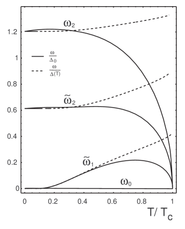
Figure 2: Collective frequencies of the neutron ${}^{3}P_{2}$ condensate at $q=0$ in units of $\Delta_{0}\equiv\Delta\left(T=0\right)$ and in units of $\Delta\left(T\right)$ versus reduced temperature in the BCS approximation.

V Discussion and conclusion

Since the equilibrium state of the condensate corresponds to $M=0$ the variables $B_{0}^{\left(1,2\right)}$ are associated with the broken gauge symmetry. In Fig. 2, the lowest curve $\omega_{0}=0$ represents the corresponding Goldstone’s mode $\omega=\omega_{0}\left(\mathbf{q}\right)$ at $q=0$. The natural appearance of this mode is caused by spontaneous breaking of the baryon number owing to the Cooper condensation. The collective motion of the condensate in this wave is a periodic variation of the total phase without a change of the order parameter structure. The previous analysis L11a has shown that, at $q>0$, the Goldstone’s mode is anisotropic and strongly renormalized by the Fermi-liquid interactions. The sound velocity is found strongly dependent on the Landau parameters describing the residual particle-hole interactions.

It was expected Bed that the spontaneous breaking of rotational invariance owing to the ${}^{3}P_{2}$ pairing leads to the appearance of three more Goldstone bosons (angulons). We found no Goldstone modes associated with the breaking of rotational symmetry. In our model, the variables $B_{\pm 1}^{\left(1,2\right)}$ are associated with a flapping motion of the total angular momentum which represents the nonunitary state, where the excited Cooper pairs have a nonzero average spin. In other words this can be imagined as a departure of the symmetry axis of the bound pair about the symmetry axis of the equilibrated condensate. This is equivalent to oscillations of the preferred direction of the Cooper pair about the axis of the energy gap in the quasiparticle energy. The quasiparticle readjustment can not follow this rapid motion. As a result instead of the angulons we found the modes $\tilde{\omega}_{1}$ which correspond to $M=\pm 1$ and look like the ”normal-flapping” mode in ³He-A W . The temperature variation of $\tilde{\omega}_{1}$ is naturally explained: the moment of inertia associated with the quasiparticles declines owing to a decrease of number of thermal quasiparticles along with a lowering of the temperature. At zero temperature the restoring force is expected to vanish along with the number of thermal quasiparticles. Accordingly, the frequency of these modes passes through a maximum and tends to zero for $T\rightarrow 0$.

The variables $B_{\pm 2}^{\left(1,2\right)}$ are found as $q\rightarrow 0$ to oscillate at frequencies $\omega=\omega_{2}\left(y\right)$ and $\omega=\tilde{\omega}_{2}\left(y\right)$ with $\omega_{2}\left(T=0\right)=1.20\Delta\left(0\right)$ and $\tilde{\omega}_{2}\left(T=0\right)=0.61\Delta\left(0\right)$. To understand the nature of these excitations we introduce three spontaneous orbital axes of the gap $\mathbf{j},\mathbf{k},\mathbf{l}$ with $\mathbf{j}\perp\mathbf{k}$ and $\mathbf{l}=\mathbf{j\times k}$ being the symmetry axis. Then the equilibrium gap matrix of the ${}^{3}P_{2}$ condensate with $M=0$ at the point $\mathbf{n}$ on the Fermi surface can be written as

$$\hat{D}=\frac{1}{\sqrt{2}}\left(\begin{array}[c]{cc}\left(\mathbf{j}-i\mathbf{k}\right)\mathbf{n}&2\mathbf{ln}\\ 2\mathbf{ln}&-\left(\mathbf{j}+i\mathbf{k}\right)\mathbf{n}\end{array}\right).$$

Variation of this matrix caused by the modes with $M=\pm 2$ is of the form (we omit the superscript in $B_{2}^{1}$)

$$\delta\hat{D}_{\left|2\right|}=e^{i\omega t}\left(\begin{array}[c]{cc}-B_{2}\left(\mathbf{j}+i\mathbf{k}\right)\mathbf{n}&0\\ 0&B_{-2}\left(\mathbf{j}-i\mathbf{k}\right)\mathbf{n}\end{array}\right).$$

This form indicates that the oscillations occur in the plane $(\mathbf{j},\mathbf{k})$. The admixture of the $\delta\hat{D}_{2}$ to $\hat{D}$ can be imagined as a clapping motion of $\mathbf{j}$ and $\mathbf{k}$ about their equilibrium relative angle of $\pi/2$.

According to Eqs. (46), in the vector channel of excitation one has $B_{-2}=B_{2}^{\ast}$, and the excited state $\mathfrak{D}=\hat{D}+\delta\hat{D}_{\left|2\right|}$ is unitary. This means the $\omega_{2}$ excitations correspond to the states with no net spin polarization. In the axial-vector channel, from Eqs. (58) one obtains $B_{-2}=-B_{2}^{\ast}$, and the excited state $\mathfrak{D}=\hat{D}+\delta\hat{D}_{\left|2\right|}$ is nonunitary, i.e. for $\tilde{\omega}_{2}$ excitations the average spin expectation value is nonzero. (The same takes place for the flapping mode $\tilde{\omega}_{1}$.) This allows one to term these oscillations by spin waves.

The flapping mode $\tilde{\omega}_{1}$ needs special discussion. The oscillation frequency for this mode is small, $\tilde{\omega}_{1}^{2}\ll 4\Delta^{2}$. This allows one to neglect $\omega^{2}$ in the integrand of Eq. (44) thus obtaining

$$\mathcal{I}_{0}\left(\tilde{\omega}_{1}\mathbf{,n}\right)\simeq\tilde{I}_{0}\left(\mathbf{n}\right)\equiv\frac{\Delta^{2}}{4}\int_{-\infty}^{\infty}\frac{d\varepsilon}{E^{3}}\tanh\frac{E}{2T}\text{ }$$ (66)

with $E=\sqrt{\varepsilon^{2}+\Delta^{2}\bar{b}^{2}\left(n_{3}\right)}$.

After this simplification we find  the analytic solution of the form

$$\tilde{\omega}_{1}^{2}=\Delta^{2}\frac{2\int_{0}^{1}dn_{3}\left[3n_{3}^{2}\left(1-n_{3}^{2}\right)\tilde{I}_{0}-\left(1-3n_{3}^{2}\right)A\right]}{3\int_{0}^{1}dn_{3}\left(1+n_{3}^{2}\right)\tilde{I}_{0}}.$$ (67)

In previous works L10c the right-hand side of Eq. (67) was evaluated in the average-angle approximation assuming that the anisotropic gap in the quasiparticle energy is replaced by its average-angle magnitude, $\bar{b}^{2}\Delta^{2}\left(T\right)\rightarrow\Delta^{2}\left(T\right)$. Such approach results in $\tilde{\omega}_{1}^{\mathsf{av}}=\Delta\left(T\right)/\sqrt{5}$ with a simple temperature dependence of the excitation energy only through the gap amplitude. Owing to the gap anisotropy the energy of the spin density oscillations depends more dramatically on the temperature, as shown in Fig. 2. As can be seen the gap anisotropy leads to a strong decreasing of the level energy along with a lowering of the temperature. This is to suppress substantially the neutrino energy losses caused by the spin wave decays because the rate of neutrino losses is strongly dependent on the wave energy. Since we have found also the new collective modes, which are kinematically able to decay into neutrino pairs, the problem of neutrino emissivity of the ${}^{3}P_{2}$ condensate at lowest temperatures is to be revisited.

It is necessary to note finally that the Fermi-liquid effects can somewhat modify the collective frequencies as compared to that found in the BCS approximation.

Appendix A Functions used

We denote as $L_{X,X}\left(\omega,\mathbf{q;p}\right)$ the analytical continuation of the Matsubara sums:

$$L_{XX^{\prime}}\left(\omega_{\eta},\mathbf{p+}\frac{\mathbf{q}}{2}\mathbf{;p-}\frac{\mathbf{q}}{2}\right)=T\sum_{\kappa}X\left(P_{+}\right)X^{\prime}\left(P_{-}\right),$$ (1)

where $X,X^{\prime}\in G,F,G^{-}$ and operate with integrals over the quasiparticle energy:

$$\mathcal{I}_{XX^{\prime}}\left(\omega,\mathbf{n,q};T\right)\equiv\int_{-\infty}^{\infty}d\varepsilon_{p}L_{XX^{\prime}}\left(\omega,\mathbf{p+}\frac{\mathbf{q}}{2}\mathbf{,p-}\frac{\mathbf{q}}{2}\right).$$ (2)

These are functions of $\omega$, $\mathbf{q}$ and the direction of a quasiparticle momentum $\mathbf{n}$, except the function $\mathcal{I}_{G_{N}G_{N}^{-}}$ which is to be evaluated for $\omega=0$, $\mathbf{q}=0$ in all cases. One can easily check that

$$\mathcal{I}_{G^{-}G}=\mathcal{I}_{GG^{-}}~{},~{}\mathcal{I}_{GF}=-\mathcal{I}_{FG}~{},~{}\mathcal{I}_{G^{-}F}=-\mathcal{I}_{FG^{-}}~{}.$$ (3)

We use also the following relations valid for arbitrary $\omega,\mathbf{q},T$

$$\mathcal{I}_{G^{-}F}=\frac{\omega-\mathbf{qv}}{2\Delta}\mathcal{I}_{FF}~{},$$ (4)

$$\mathcal{I}_{FG}=\frac{\omega+\mathbf{qv}}{2\Delta}\mathcal{I}_{FF}~{},$$ (5)

and

$$\mathcal{I}_{GG^{-}}-\mathcal{I}_{G_{N}G_{N}^{-}}+\bar{b}^{2}\mathcal{I}_{FF}=A+\frac{\omega^{2}-\left(\mathbf{qv}\right)^{2}}{2\Delta^{2}}\mathcal{I}_{FF},$$ (6)

The function $A\left(\mathbf{n}\right)$ is defined by Eq. (28) and can be written as

$$A\left(\mathbf{n}\right)=\left[\mathcal{I}_{GG^{-}}-\mathcal{I}_{G_{N}G_{N}^{-}}+\bar{b}^{2}\mathcal{I}_{FF}\right]_{\omega=0,\mathbf{q}=0}.$$ (7)

The explicit form of this function is given in Eq. (43).

Appendix B Eigenmodes in ³He-B

In the liquid ³He-B, the pairing occurs owing to the exchange central interaction which is independent of the total angular momentum of the bound pair, $J$. In this case the interaction in the channel $S=1$, $L=1$ can be written in the same form as given in Eq. (17) but the summation over the total angular momentum $J=0,1,2$ is to be added with $-J\leq M\leq J$. Then instead of Eqs. (47) and (59) one obtains, respectively,

$$\det\left|~{}\left\langle\left(\mathbf{b}_{J^{\prime}M^{\prime}}\mathbf{b}_{JM}^{\ast}-\delta_{JJ^{\prime}}\delta_{MM^{\prime}}\mathbf{\bar{b}}^{2}\right)A\right\rangle\right.$$

$$\left.+\left\langle\left[\left(\frac{\omega^{2}-\left(\mathbf{qv}\right)^{2}}{2\Delta^{2}}-2\bar{b}^{2}\right)\left(\mathbf{b}_{J^{\prime}M^{\prime}}\mathbf{b}_{JM}^{\ast}\right)+2\left(\mathbf{b}_{JM}^{\ast}\mathbf{\bar{b}}\right)\left(\mathbf{b}_{J^{\prime}M^{\prime}}\mathbf{\bar{b}}\right)\right]\mathcal{I}_{0}\right\rangle\right|=0,$$ (8)

and

$$\det\left|~{}\left\langle\left(\mathbf{b}_{J^{\prime}M^{\prime}}\mathbf{b}_{JM}^{\ast}-\delta_{JJ^{\prime}}\delta_{MM^{\prime}}\mathbf{\bar{b}}^{2}\right)A\right\rangle\right.$$

$$\left.+\left\langle\left[\frac{\omega^{2}-\left(\mathbf{qv}\right)^{2}}{2\Delta^{2}}\left(\mathbf{b}_{J^{\prime}M^{\prime}}\mathbf{b}_{JM}^{\ast}\right)-2\left(\mathbf{b}_{JM}^{\ast}\mathbf{\bar{b}}\right)\left(\mathbf{b}_{J^{\prime}M^{\prime}}\mathbf{\bar{b}}\right)\right]\mathcal{I}_{0}\right\rangle\right|=0,$$ (9)

where the vectors $\mathbf{b}_{JM}$ for $J=2$ are given by Eq. (19) and for $J=0,1$ one has

$$\mathbf{b}_{0,0} =\left(-n_{1},-n_{2},-n_{3}\right),$$

$$\mathbf{b}_{1,0} =\sqrt{\frac{3}{2}}\left(in_{2},-in_{1},0\right),$$

$$\mathbf{b}_{1,1} =\mathbf{b}_{1,-1}^{\ast}=\sqrt{\frac{3}{4}}\left(-n_{3},-in_{3},n_{1}+in_{2}\right),$$ (10)

In ³He-B, the equilibrium state of the condensate corresponds to the bound pairs with $J=0$. The order parameter in such a system is $\mathbf{\bar{b}}=\mathbf{b}_{0,0}$, and the energy gap $\Delta\bar{b}\left(\mathbf{n}\right)=\Delta$ is isotropic ($\bar{b}^{2}=1$). The latter means that, in Eqs. (8), (9), the functions $A$ and $\mathcal{I}_{0}$ are isotropic and can be moved beyond the integrals. Using also the orthogonality condition, $\left\langle\mathbf{b}_{JM}\mathbf{b}_{J^{\prime}M^{\prime}}^{\ast}\right\rangle=\delta_{JJ^{\prime}}\delta_{MM^{\prime}}$, we find

$$~{}\left\langle\mathbf{b}_{J^{\prime}M^{\prime}}\mathbf{b}_{JM}^{\ast}-\delta_{JJ^{\prime}}\delta_{MM^{\prime}}\mathbf{\bar{b}}^{2}\right\rangle=0~{},$$ (11)

thus obtaining from Eq. (8) the dispersion equation

$$\det\left|\left\langle\left(\frac{\omega^{2}-\left(\mathbf{qv}\right)^{2}}{2\Delta^{2}}-2\right)\left(\mathbf{b}_{J^{\prime}M^{\prime}}\mathbf{b}_{JM}^{\ast}\right)+2\left(\mathbf{b}_{JM}^{\ast}\mathbf{\bar{b}}\right)\left(\mathbf{b}_{J^{\prime}M^{\prime}}\mathbf{\bar{b}}\right)\right\rangle\right|=0.$$ (12)

We examine solutions to this equation for $\mathbf{q}=0$. A straightforward calculation of the angle integrals results in

$$\left\langle\left(\mathbf{b}_{JM}^{\ast}\mathbf{\bar{b}}\right)\left(\mathbf{b}_{J^{\prime}M^{\prime}}\mathbf{\bar{b}}\right)\right\rangle=\delta_{JJ^{\prime}}\delta_{MM^{\prime}}\left(\delta_{J0}\delta_{M0}+\frac{2}{5}\delta_{J2}\right).$$ (13)

Implying $J=0,1,2$ and $\left|M\right|\leq J$ we obtain the dispersion equation

$$\Omega^{2}\left(\Omega^{2}-1\right)^{3}\left(\Omega^{2}-\frac{3}{5}\right)^{5}=0,$$ (14)

where we denote

$$\Omega=\frac{\omega}{2\Delta\left(T\right)}.$$ (15)

From this equation we find one mode with frequency $\omega=0$, five degenerate modes with frequency $\omega=\sqrt{12/5}\Delta$, and three degenerate modes with frequency $\omega=2\Delta$. In the same way starting from Eq. (9) we obtain the dispersion equation for eigenmodes of spin density and spin-current density which can be excited by the axial-vector external field

$$\left(\Omega^{2}-1\right)\left(\Omega^{2}\right)^{3}\left(\Omega^{2}-\frac{2}{5}\right)^{5}=0.$$ (16)

From this equation we find one mode with frequency $\omega=2\Delta$, five degenerate modes with frequency $\omega=\sqrt{8/5}\Delta$, and three degenerate modes with frequency $\omega=0$. This completes the enumeration of the 18 B-phase collective modes for $\mathbf{q}=0$. Note these results are identical to ones obtained earlier in Refs. Wolfe1 , Ketterson .

Appendix C Critical temperature

Combining Eq. (30) for $T>0$ with the same equation for $T=0$ one can obtain the equality

$$\left\langle\bar{b}^{2}\int_{-\infty}^{\infty}d\varepsilon\left[\left(\varepsilon^{2}+\Delta_{0}^{2}\bar{b}^{2}\right)^{-1/2}-\left(\varepsilon^{2}+\Delta^{2}\bar{b}^{2}\right)^{-1/2}\right]\right\rangle=-\left\langle 2\bar{b}^{2}\int_{-\infty}^{\infty}\frac{d\varepsilon}{E}\left(e^{E/T}+1\right)^{-1}\right\rangle,$$ (17)

where $E=\sqrt{\varepsilon^{2}+\Delta^{2}\bar{b}^{2}}$. Performing the integral in the left-hand side we find

$$\ln\frac{\Delta_{0}}{\Delta}=2\left\langle\bar{b}^{2}\int_{0}^{\infty}\frac{dx}{\sqrt{x^{2}+y^{2}\bar{b}^{2}}}\left(e^{\sqrt{x^{2}+y^{2}\bar{b}^{2}}}+1\right)^{-1}\right\rangle.$$ (18)

The internal integral in the right-hand side is calculated in Ref. lif . Close to the transition point $T\rightarrow T_{c}$ one obtains

$$\ln\frac{\Delta_{0}}{\Delta}=\left\langle\bar{b}^{2}\left(\ln\frac{\pi T}{\gamma\Delta\bar{b}}+\frac{7\zeta\left(3\right)}{8\pi^{2}}\frac{\Delta^{2}}{T^{2}}\right)\right\rangle,$$ (19)

where $\ln\gamma=C=0.577$ is Euler’s constant. According to this equation the gap vanishes at the temperature

$$T_{c}=\Delta_{0}\frac{\gamma}{\pi}\exp\left\langle\bar{b}^{2}\ln\bar{b}\right\rangle.$$ (20)

We evaluate this relation for $\bar{b}^{2}=\left(1+3n_{3}^{2}\right)/2$ to find

$$\frac{T_{c}}{\Delta_{0}}=\frac{\sqrt{2}\gamma}{\pi}e^{\frac{1}{27}\pi\sqrt{3}-\frac{1}{2}}=0.595.$$ (21)

References

(1)P. Haensel, Nucl. Phys. A 301, 53 (1978).
(2)L. B. Leinson, V. N. Oraevsky, and V. B. Semikoz, Physics Lett.
B, 209, 80 (1988).
(3)C. J. Horowitz and K. Wehrberger, Nucl. Phys. A 531, 665 (1991).
(4)C. J. Horowitz and K. Wehrberger, Phys. Lett. B 266,
236 (1991).
(5)E. Braaten and D. Segel, Phys.Rev. D 48, 1478 (1993).
(6)F. Matera and V. Yu. Denisov, Phys. Rev. C 49, 2816 (1994).
(7)S. Reddy, M. Prakash, J. M. Lattimer, and J. Pons, Phys. Rev. C
59, 2888 (1999).
(8)L. B. Leinson, Phys. Lett. B 469, 166 (1999).
(9)L. B. Leinson, Phys. Lett. B 473, 318 (2000).
(10)L. B. Leinson, Nucl. Phys. A 687, 489 (2001).
(11)V. Greco, M. Colonna, M. Di Toro, and F. Matera, Phys. Rev. C
67, 015203 (2003).
(12)C. Providência, L. Brito, A. M. S. Santos, D. P. Menezes, and
S. S. Avancini, Phys. Rev. C. 74, 045802 (2006).
(13)D. G. Yakovlev, A. D. Kaminker, and K. P. Levenfish, Astron.
Astrophys. 343, 650 (1999).
(14)L. B. Leinson, Phys. Rev. C 81, 025501 (2010).
(15)L. B. Leinson, Phys. Rev. C 83, 055803 (2011).
(16)L. B. Leinson, Phys. Lett. B 689, 60 (2010).
(17)L. B. Leinson, Phys. Rev. C 82, 065503 (2010).
(18)L. B. Leinson, Phys. Lett. B 702, 422 (2011).
(19)L. B. Leinson, Phys. Rev. C 84, 045501 (2011).
(20)M. Hoffberg, A. E. Glassgold, R. W. Richardson, M. Ruderman,
Phys. Rev. Lett. 24, 775 (1970).
(21)M.V. Zverev, J. W. Clark, and V. A. Khodel, Nucl. Phys. A
720, 20 (2003).
(22)V. A. Khodel, J. W. Clark, and M.V. Zverev, Phys. Rev. Lett.
87, 031103 (2001).
(23)V. A. Khodel, J. W. Clark, and M.V. Zverev, e:Print: arXiv:nucl-th/0203046.
(24)P. Wölfe, Phys. Rev. Lett. 30, 1169 (1973).
(25)P. Wölfe, Phys. Rev. Lett. 31, 1437 (1973).
(26)K. Maki and H. Ebisawa, J.Low Temp. Phys. 15, 213 (1974).
(27)R. Combescot, Phys. Rev. A 10, 1700 (1974).
(28)R. Combescot, Phys. Rev. Lett. 33, 946 (1974).
(29)H. Ebisawa and K. Maki, Prog. Theor. Phys. 51, 337 (1974).
(30)P. Wölfe, Physica B 90, 96 (1977).
(31)P. Wölfe, Phys. Rev. Lett. 37, 1279 (1976).
(32)L. Amundsen and E. Østgaard, Nucl. Phys. A 442, 163 (1985).
(33)A. I. Larkin and A. B. Migdal, Zh. Eksp. Teor. Fiz.
44, 1703 (1963) [Sov. Phys. JETP 17, 1146 (1963)].
(34)A. J. Leggett, Phys. Rev. 147, 119 (1966).
(35)A. J. Leggett, Rev. Mod. Phys, 47, 331 (1975)
(36)J. B. Ketterson and S. N. Song, Superconductivity, (University press, Cambridge, 1999), p. 414.
(37)P. F. Bedaque, G. Rupak, and M. J. Savage, Phys. Rev. C
68, 065802 (2003).
(38)E. M. Lifshitz, L. P. Pitaevskii, Statistical Physics,
Part 2 (Pergamon Press, Oxford, 1980).