Type-Ia SUPERNOVA REMNANT SHELL AT $z=3.5$ SEEN IN THE THREE SIGHTLINES TOWARD THE GRAVITATIONALLY LENSED QSO B1422+231

Abstract

Using the Subaru 8.2m Telescope with an IRCS Echelle spectrograph, we obtained high-resolution ($R=$10,000) near-infrared (1.01-1.38$\mu$m) spectra of images A and B of the gravitationally lensed QSO B1422+231 ($z=3.628$) consisting of four known lensed images. We detected Mg II absorption lines at $z=3.54$, which show a large variance of column densities ($\sim$0.3 dex) and velocities ($\sim$10 km s^-1) between the sightlines A and B with a projected separation of only $8.4h_{70}^{-1}$ pc at the redshift. This is the smallest spatial structure of the high-$z$ gas clouds ever detected after Rauch et al. found a 20-pc scale structure for the same $z=3.54$ absorption system using optical spectra of images A and C. The observed systematic variances imply that the system is an expanding shell as originally suggested by Rauch et al. By combining the data for three sightlines, we managed to constrain the radius and expansion velocity of the shell ($\sim$50-100 pc, 130 km s^-1), concluding that the shell is truly a supernova remnant (SNR) rather than other types of shell objects, such as a giant H II region. We also detected strong Fe II absorption lines for this system, but with much broader Doppler width than that of $\alpha$-element lines. We suggest that this Fe II absorption line originates in a localized Fe II-rich gas cloud that is not completely mixed with plowed ambient interstellar gas clouds showing other $\alpha$-element low-ion absorption lines. Along with the Fe richness, we conclude that the SNR is produced by an SNIa explosion.

1. Introduction

Gravitationally lensed QSOs provide us precious opportunities to study spatial structures of high-$z$ gas clouds which intersect the multiple sightlines toward the QSO (e.g., Weymann & Foltz, 1983; Foltz et al., 1984; Smette et al., 1995; Rauch et al., 1999, 2001a, 2001b, 2002; Kobayashi et al., 2002; Churchill et al., 2003a; Ellison et al., 2004; Lopez et al., 2005; Monier et al., 2009). By comparing the profiles of absorption lines between multiple sightlines, we can study the density and velocity gradients of intersecting gas clouds directly even at high redshift. Such spatial properties of absorbing gas at high redshift may provide a key to understand the galaxy formation processes.

The statistical studies of absorption line systems with the gravitationally lensed QSOs have revealed that the Mg II systems, which trace low-ionization systems are relatively small ($<$ a few hundred pc) and have clumpy spatial structures (Rauch et al., 2002; Ellison et al., 2004), in contrast to the C IV systems which are typically a few kpc in size and have fewer structures (Rauch et al., 2001a; Ellison et al., 2004). Studies of single line-of-sight observations and CLOUDY photoionization modeling (Ferland et al., 1998) also suggest that the Fe-rich low-ionization systems should be as small as 10 pc (Rigby et al., 2002; Narayanan et al., 2008). Thus, low-ionization systems appear to have small clumpy spatial structures that directly relate to star forming activities, such as giant molecular clouds. It is important to investigate their spatial properties with multiple sightlines of gravitationally lensed QSOs, since only the gravitational lens can directly reveal fundamental parameters such as the size and kinematics of gas clouds.

The quadruple gravitationally lensed QSO B1422+231 (Patnaik et al., 1992) is one of the best objects for such a study because of the relatively small separations among multiple sightlines due to the large distance between the lense galaxy ($z=0.339$; Kundic et al., 1997; Tonry, 1998) and the QSO ($z=3.628$). This QSO has been observed frequently as one of the most luminous gravitationally lensed high-$z$ QSOs (Bechtold & Yee, 1995; Songaila & Cowie, 1996; Petry et al., 1998; Rauch et al., 1999, 2001a, 2001b). Rauch et al. (1999, , hereafter RSB99) obtained high-resolution optical spectra of images A and C of B1422+231 using Keck HIRES (Vogt et al., 1994) and detected C IV, Si IV, C II, Si II, and O I absorption lines from the $z=3.54$ absorption system originally identified by Songaila & Cowie (1996) with strong Ly$\alpha$ and Ly$\beta$ absorption lines. The projected separation between A and C sightlines is only 22.2$h^{-1}_{70}$pc at the redshift. RSB99 suggested that the absorption system is an expanding shell of mass ejection or supernova remnants (SNRs) by analyzing the differences of the absorption profiles of lower ionization species between the images A and C.

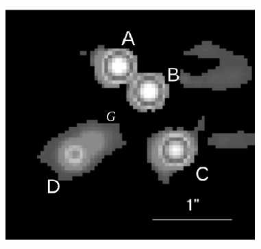
Figure 1.— HST F555W image of B1422+231 from CASTLES homepage (http://www.cfa.harvard.edu/castles). North is up, east is to the left. Four white point sources show gravitationally lensed images A, B, C and D. The extended object (G) to the northwest of image D shows the lensing galaxy of this system. We obtained spectra of the two brightest and closest components, A and B.

In this paper, we report the results of the Subaru near-infrared spectroscopic observations of images A and B of B1422+231. Previous studies of low ionization gas with Mg II QSO absorption lines were limited to the optical wavelength range and thus to redshifts $<2.5$, beyond which this transition moves into the infrared waveband. Thanks to the advent of highly sensitive near-infrared high-resolution spectroscopy with 8-10 m class telescope, it is possible now to study this unexplored redshift range. We are conducting a systematic high-resolution spectroscopic survey of high-$z$ Mg II systems with the Subaru IRCS Echelle spectrograph. We observed B1422+231 as one of the initial targets, and detected Mg II doublet and Fe II absorption lines for the $z=3.54$ system. Moreover, we succeeded in spatially resolving spectra of images A and B owing to the high spatial resolution in the infrared and the very good seeing of the Subaru Telescope site. This paper is composed as following. The details of our observations are summarized in §2. The data reduction and calibration of spectra are described in §3. In §4, we show the properties of detected Mg II and Fe II absorption lines. We interpret the properties as signatures of a Type Ia supernova (SN Ia) remnant, which is discussed in §5 in detail. §6 is the summary of this paper. We adopt a standard cosmology with $\Omega_{\Lambda}=0.7$, $\Omega_{m}=0.3$, $\Omega_{k}=0$ and $H_{0}=70h_{70}=70$ km s^-1 Mpc^-1 throughout this paper.

2. Observation

We observed images A and B of B1422+231 (Figure 1) using Subaru 8.2m Telescope (Iye et al., 2004) with IRCS Echelle spectrograph (Tokunaga et al., 1998; Kobayashi et al., 2000) in $Y$ (1.01$-$1.19$\mu$m) and $J$ (1.16$-$1.38$\mu$m) bands. The data were obtained on 2003 February 13 and 2002 April 28 for $Y$ and $J$ bands, respectively. The weather condition for both observing runs was photometric and the seeing was good ($\sim 0^{{}^{\prime\prime}}.5$) during observations for both bands. The integration time per frame was 600 sec, and the total integration time was 9000 s and 9600 s for $Y$ and $J$ bands, respectively. The slit widths were $0^{{}^{\prime\prime}}.60$ and $0^{{}^{\prime\prime}}.30$, and corresponding spectral resolutions ($R=\lambda/\Delta\lambda$) were $5,000$ and $10,000$ for $Y$ and $J$ bands, respectively, while the slit length was $3^{{}^{\prime\prime}}.47$ for both observations. Although we used the Subaru Adaptive Optics 36-elements (AO 36) system (Takami et al., 2004) for the $Y$-band observation, the improvement of image quality was not good enough that we used the wider slit. The slit position angle (P.A.) was set at P.A. = $39^{\circ}_{.}2$ to put both A and B images on the slit simultaneously. The telescope was nodded by $1^{{}^{\prime\prime}}.5$ arcsec along the A$-$B direction as shown in Figure 2 between alternating frames to offset the sky emission in the subsequent data reduction. We call the frames for positions “a” and “b” as shown in Figure 2. We also observed a standard star, 10 Boo, for flux calibration and removal of telluric absorption lines for both bands. The airmass of the target was distributed in a wide range from 1.0 to 1.5 for both bands, while that of the standard star was about 1.0 and 1.5 for $Y$ and $J$ bands, respectively.

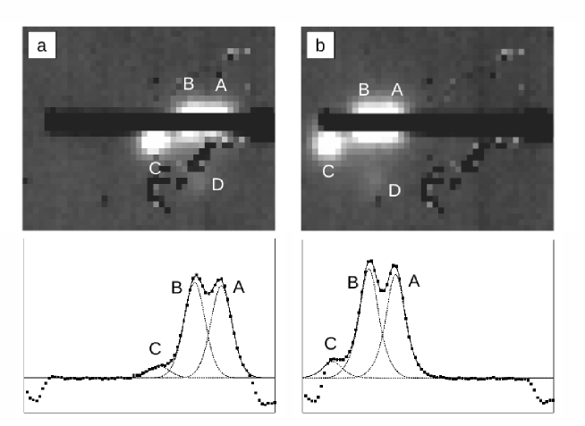
Figure 2.— Upper panels: the slitviewer $K$-band images obtained during the echelle observation. These are raw images with an integration time of 120 s without corrections for hot/bad pixels. The pixel scale is $0^{{}^{\prime\prime}}.075$ pixel^-1. The horizontal black thick bar near the center of the images is the shadow of the slit, and four point sources which are seen in white are the images A, B, C and D of B1422+231. The left and right panels correspond to the dither patterns “a” and “b” (see the text for detail). The contamination of image C in the slit is slightly seen in this image. Lower panels: the spatial profiles of the spectra along the slit. Points show the observed data. Dotted lines show fitted profiles for each image A, B, and C, while thick lines show the combined profile of the three images. To show the spatial profile clearly, the data are averaged in the dispersion axis over one cross-disperser order (order 44 of $J$ band). The hollows at both edges show the areas beyond the end of the slit, which are not used for the profile fitting.

3. Data Analysis

3.1. Reduction

We used IRAF for data reduction following standard procedures. First, we subtracted “b” frames from corresponding “a” frames to cancel out the dark counts and the sky OH emission lines. All the subtracted frames were combined after the flat-fielding correction and hot/bad pixel correction. Then, we extracted two-dimensional (2D) spectra with the spatial axis along the slit and the dispersion axis perpendicular to the slit for each cross-disperser order using IRAF task “apall” in the “echelle” package. The 2D spectra of each order were combined after applying the wavelength calibration with Argon lamp spectra, which were obtained after the observation.

3.2. Deconvolution of A and B Spectra

The lower panel of Figure 2 shows the spatial profile of the 2D spectra of B1422+231 along the slit. The images A and B are almost resolved, but the overlap is not negligible. Image C, which is not a target of this study, is contaminated slightly in the spatial profiles. To obtain precise one-dimensional (1D) spectra of images A and B from the 2D spectra, we fitted the observed spatial profile with the point spread functions (PSFs) of the three images pixel by pixel in the dispersion axis. This method is similar to that of Lopez et al. (2005), who also observed the multiple images of a gravitational-lensed QSO in a slit simultaneously.

Because the tail of PSF was found to decline slower than that of a Gaussian function, we assumed the following double Gaussians as the form of a PSF:

$$f_{i}(x,\lambda)=\frac{a_{i}(\lambda)}{2}\left(\exp\Big{[}-\frac{(x-b_{i})^{2}}{\sigma_{s}^{2}}\Big{]}+\exp\Big{[}-\frac{(x-b_{i})^{2}}{\sigma_{d}^{2}}\Big{]}\right),$$ (1)

where $i=$A, B, C are the indices for the lensed images, $x$ is the coordinate of pixels in the spatial axis, $a_{i}(\lambda)$ is the peak value of each image at wavelength $\lambda$, $b_{i}$ is the center position of each image, and $\sigma_{s}$ and $\sigma_{d}$ are the width of each Gaussian function ($\sigma_{s}<\sigma_{d}$ ; the subscripts “s” and “d” mean sharp and diffuse, respectively). This function was found to fit the observed profile precisely as shown in the lower panel of Figure 2.

The parameters $b_{i}$, $\sigma_{s}$, and $\sigma_{d}$ have to be fixed for linear fitting, which is necessary to converge the fit for observed profiles with low signal to noise ratio (S/N). These parameters are successfully determined from the fit of the high S/N spatial profile made by summing the spatial profiles for 50 pixels along the dispersion axis. The “fit” command of gnuplot was used for the fitting procedure. Though this program is not designed for numerical fitting, it is good enough to conduct the linear fitting. The flux density count at wavelength $\lambda$ for image $i$ was determined by the integral of the PSF $f_{i}(x,\lambda)$ along the spatial axis, which can be analytically calculated as $\sqrt{\pi}a_{i}(\lambda)(\sigma_{s}+\sigma_{d})/2$ for double Gaussians. When all the fitting parameters are determined for the entire wavelength range, the final 1D spectrum of each image is constructed by plotting the flux density count along the dispersion axis.

Figure 3.— Upper panel: the whole $Y$- and $J$-band spectra of images A (lower spectra) and B (upper spectra) of B1422+231. The observed spectra were telluric-corrected and smoothed with an 11 pixel ($\sim 3$Å) box car to clearly show the spectra with an effective spectral resolution of R$\sim$4,000. The bumps on the continuum are broad Mg II and Fe II emission lines from the QSO itself at $z=$3.628. The vertical bars show the expected positions of absorption lines associated with the $z=3.54$ system: solid and dashed lines show the positions of the detected and non-detected lines, respectively. Lower panel: the telluric absorption spectrum in the same wavelength range. This is made by normalizing the spectrum of the standard star, 10 Boo, after removing two hydrogen absorption lines (Pa$\beta$ and Pa$\gamma$) with Voigt profile fitting.

Figure 4.— Upper panel: the normalized spectrum of image A around Mg II doublet lines of the $z=3.54$ system after the telluric corrections. Lower panel: the normalized spectrum of the standard star 10 Boo, showing the telluric absorption lines. The strong O₂ absorption band at around 12690 Å apparently affects the detection and profiles of components 1 and 2 of Mg II $\lambda$2796.

3.3. 1D Spectra

Many telluric absorptions of e.g., water (H₂O) and oxygen (O₂) plus emission lines of OH appear on the near-infrared spectra for ground-based observations. Although the emission lines are removed by the substraction of images of alternative pointing (§3.1), the absorption lines are still superposed on the extracted spectra of the object. For both bands, we removed the telluric absorption lines by dividing the object spectra by that of a A0 standard star, 10 Boo, which has few intrinsic absorption lines except for two strong hydrogen absorption lines : Pa$\gamma$ ($\sim$ 10935 Å) in $Y$ band (order 51 and 52) and Pa$\beta$ ($\sim$ 12815Å) in $J$ band (order 44). Before the division, we removed these hydrogen lines by fitting with Voigt profile, and scaling the telluric absorption lines to correct the airmass difference (§2). Figure 3 shows the flux calibrated spectra of images A and B. We used the continuum of the telluric standard star 10 Boo (5.67 mag in $J$-band from SIMBAD) for flux calibration, assuming the effective temperature of 9480 K.

To avoid the influence of many bumps due to Fe II and Mg II emission lines from the QSO itself on the continuum fitting, the normalized absorption spectra were made by fitting the continuum in a velocity range of $\pm 500$ km s^-1, which is narrower than the velocity widths of the emission lines ($\sim 1000$ km s^-1), around the detected absorption lines using spline3 function.

Heliocentric corrections of $-$21.89 km s^-1 and $-$5.18 km s^-1 were applied to $Y$- and $J$-band spectra, respectively. By comparing the detected Mg II absorption lines with C II and Si II absorption lines for image A (RSB99), a residual offset of $-$3.4 km s^-1 (about a half pixel) was found in our $J$-band spectrum. We shifted the absorption line spectrum by +3.4 km s^-1 to match the wavelength of the C II/Si II absorption lines with those derived by RSB99 because their spectral resolution ($R=$70,000, $\Delta v=4.4$ km s^-1) is much better than ours ($R=$10,000, $\Delta v=30$ km s^-1). This offset is likely to come from the slight change of the instrument setting that occurred between the observation of targets and the acquisition of the Argon lamp spectrum. For $Y$-band data, no absorption lines that have obvious peaks as Mg II absorption lines of the $z=3.54$ system were detected. Therefore, we did not shift the spectra after the heliocentric correction.

4. $z=3.54$ System

Table 1Detected Mg II absorption lines.

Image	Comp	$W_{r}$($\lambda$2796)(Å)	$W_{r}$($\lambda$2803)(Å)	Doublet ratio
A	1	(0.020)	0.018	(1.1)
	2	(0.074)	0.052	(1.4)
	3	0.191	0.124	1.5
B	2	(0.080)	0.040	(1.6)
	3	0.111	0.056	2.0

Note. — $W_{r}$ of the components that are significantly affected by telluric absorption lines are shown with parentheses.

4.1. Velocity Components

In the final $J$-band spectrum, strong Mg II $\lambda\lambda$2796, 2803 absorption lines with two velocity components at $z=3.54$ are clearly detected for both images A and B (Figure 3). The corresponding Fe II $\lambda$2383 ($f=0.320$) and $\lambda$2600 ($f=0.2394$) absorption lines of this system are also detected in image A (Figure 3), while other Fe II absorption lines, such as $\lambda$2344 ($f=0.1142$) and $\lambda$2587 ($f=0.0691$), are not detected probably because of their small oscillator strengths. Hereafter, we will focus only on this $z=3.54$ Mg II system: the search for other systems and their results will be discussed separately in S. Kondo et al. (in preparation). Unfortunately, the Mg II $\lambda$2796 line is overlapping with the telluric O₂ band as shown in Figure 4 and the systematic uncertainty may be left in the profile of Mg II $\lambda$2796 even after the removal of the telluric absorption lines (§3.3). The impact of the telluric absorption lines will be discussed in the following subsection (§4.2) for each velocity component.

This $z=3.54$ system was first detected by Songaila & Cowie (1996) as an H I system with $N$(H I) = $2.3\times 10^{16}$cm^-2 in their high-resolution optical spectrum with Keck HIRES. Later RSB99 detected various metal absorption lines also with Keck HIRES in spatially-separated spectra of images A and C. Figure 5 shows the Mg II absorption lines of the $z=3.54$ system for both images A and B from our $J$-band data, and C II, Si II, and O I absorption lines of images A and C from RSB99’s optical data.

For the Mg II absorption lines, we clearly detected two velocity components for both images A and B at $\sim-80$ km s^-1 and $\sim+90$ km s^-1, which are identified as “component 2” and “component 3” in RSB99. The Mg II absorption line that corresponds to “component 1” is also detected at $\sim-130$ km s^-1, but only for image A (Figure 5). The rest-frame equivalent widths ($W_{r}$) of detected Mg II $\lambda\lambda$2796, 2803 absorption lines are summarized in Table 1. Note that the equivalent widths of lines that are affected by the strong telluric absorption lines are shown with parentheses. The total rest-frame equivalent width of $\lambda 2796$ for this system is calculated as 0.28Å. Therefore, this system is classified as a “weak Mg II system” which is defined as a system with $W_{r}(2796)<0.3$ Å (Churchill et al., 1999). The corresponding Fe II $\lambda 2383,\lambda 2600$ absorption lines are also detected for component 3 but only for image A as shown in Figure 6 (left panel). The Mg I absorption line is not detected for any component for both images within the uncertainty.

We fit a Voigt profile to the Mg II and Fe II absorption lines and measured the column density, the relative velocity, and the Doppler width using VPFIT(Carswell et al., 1987) and VPGUESS software assuming each velocity component is composed of just one velocity sub-component, which is a good approximation for estimating column densities from our data with the velocity resolution of $\Delta v=30$km s^-1 at most. The results are summarized in Table 2. The shown uncertainty is only that for the VPFIT fitting. For non-detected absorption lines, we calculated the $3\sigma$ upper limit of the column density from the S/N of the continuum around the absorption lines. We discuss the characteristics of the detected Mg II and Fe II absorption lines in the following.

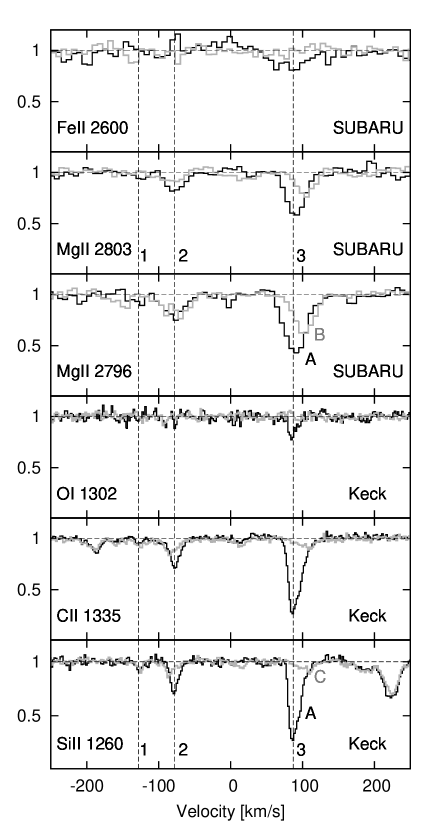
Figure 5.— Spectra of the $z=3.54$ absorption system of images A (black lines), B (gray lines for Mg II and Fe II), and C (gray lines for Si II, C II and O I) of B1422+231. The spectral resolutions are about 10,000 and 70,000 for our SUBARU data (top three panels) and RSB99’s Keck data (bottom three panels), respectively. The vertical dashed lines show the peak position of the three velocity components of image A. The velocity is relative to $z=3.53850$. The atomic species and their rest-frame wavelengths are shown at the left bottom corner of each plot.

4.2. Mg II Absorption Lines

Table 1 summarizes the Mg II doublet ratio, which is defined as $W_{r}(2796)$/$W_{r}(2803)$, for each component of each image. Where both $\lambda\lambda$2796, 2803 absorption lines are not saturated, the doublet ratio should be equal to 2 by simply reflecting the oscillator strengths. For the strongest component (component 3), the doublet ratio is found to be 1.5 for image A, while equal to 2 for image B. Therefore, the absorption line of image A may be slightly saturated while that of image B is not. Although the other weaker components are also unlikely to be saturated in view of the smaller $W_{r}(2803)$ than that for the component 3 of image B, the doublet ratios for those components show values less than 2. This is probably because $W_{r}(2796)$ of components 1 and 2 is underestimated due to the incomplete removal of the heavy telluric absorption lines that are overlapped on those components (Figure 4). Here, we discuss details of the Mg II absorption lines for each component 1, 2, and 3 .

Component 1. For this component, RSB99 shows that there is no difference between the absorption lines of images A and C, thus the same absorption profile was expected for image B, which is located in between images A and C on the sky. However, we could not detect component 1 in image B despite its existence in the spectrum of image A (Figure 5). In particular, we had expected to detect the Mg II $\lambda 2803$ absorption line because it is not affected by the strong O₂ telluric absorption lines unlike the Mg II $\lambda 2796$ absorption line. The Mg II $\lambda$2803 absorption line for component 1 is located right in between two weak telluric absorptoin lines (Figure 4) and should not be affected by the removal of the telluric absorption lines. Therefore, we conclude that the gas cloud of component 1 covers only images A and C on the sky, suggesting a small-scale sub-structure on this high-redshift cloud.

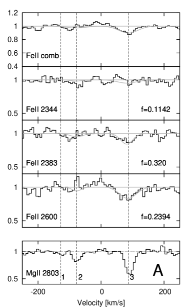
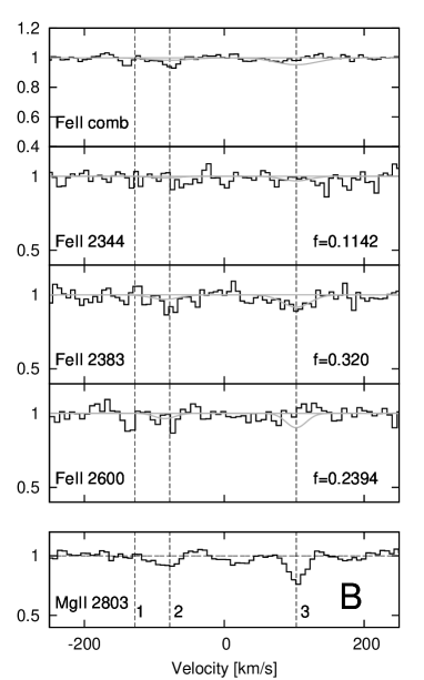
Figure 6.— Spectra of Fe II lines of the $z=3.54$ system for images A and B. The spectrum of Mg II $\lambda$2803 line is also shown at the bottom as a reference. The top spectrum “Fe II comb” shows the combined spectra of Fe II $\lambda$2344, $\lambda$2383 and $\lambda$2600. The species and the rest-frame wavelength are shown at the bottom left of each spectrum. The oscillator strength of each line from Morton (1991) is shown at the bottom right of each plot. The spectral resolution of Fe II $\lambda$ 2600 and Mg II $\lambda$2803 spectra is $R\sim 10,000$, while that of Fe II $\lambda$2383, 2344 and “Fe II comb” is $R\sim 5000$. The vertical dashed lines show the center positions of three velocity components of each images. The gray lines show the Fe II absorption profiles predicted from the Mg II profiles (see the detail in Section 4.3).

Table 2The Results of Voigt Profile Fitting with VPFIT

Species	Component	$\log N_{A}\text{(cm}^{-2}\text{)}$	$\log N_{B}\text{(cm}^{-2}\text{)}$	$v_{A}$(km s-1)	$v_{B}$(km s-1)	$b_{A}$(km s-1)	$b_{B}$(km s-1)
Mg II	1	11.9$\pm$1.9	$\cdots$	-127$\pm$16	$\cdots$	2$\pm$55	$\cdots$
	2	12.4$\pm$0.1	12.20$\pm$0.07	-78$\pm$5	-85$\pm$3	7.2$\pm$1.3	10 $\pm$ 9
		(12.5$\pm$ 0.4)		(-77$\pm$6)		(5$\pm$29)
	3	13.03$\pm$0.07	12.66$\pm$0.04	90.6$\pm$0.6	102.9$\pm$0.6	9$\pm$1	7$\pm$1
Fe II	2	$<12.1$	$<12.1$	$\cdots$	$\cdots$	$\cdots$	$\cdots$
	3	12.72$\pm$0.05	$<12.1$	83$\pm$3	$\cdots$	23 $\pm$6	$\cdots$
Mg I	2	$<11.1$	$<11.1$	$\cdots$	$\cdots$	$\cdots$	$\cdots$

Note. — The column densities, relative velocities from $z=$3.53850, and Doppler widths measured with VPFIT are shown for both line of sight A and B.

Component 2. Although we tried to fit both Mg II $\lambda\lambda$2796, 2803 lines of component 2 simultaneously, the uncertainties of the three fitting parameters (column density, redshift and Doppler width) were found to be very large and we could not get any reliable estimate. This is most likely due to the strong telluric O₂ band on the Mg II $\lambda$2796 line (Figure 4): systematic uncertainties may be left in the profile of Mg II $\lambda$2796 even after the removal of telluric absorption lines (§3-3), which is consistent with the strange doublet ratios for component 2 described above. Therefore, we used only the Mg II $\lambda$2803 line for the Voigt profile fitting for both images A and B for this component. The results are summarized in Table 2. Due to the lack of the information on Mg II $\lambda$2796, the uncertainties are fairly large especially for the Doppler width.

For image A, fortunately, we have the information on the Doppler width with a high precision from the high-resolution optical spectrum (RSB99). We tried to estimate the Doppler width of Mg II $\lambda$2803 line from those of C II (9.8 $\pm$ 0.5 km s^-1) and Si II (6.7 $\pm$ 0.5 km s^-1) lines. Generally, a Doppler width $b$ consists of thermal ingredient $b_{\text{th}}$ and turbulence ingredient $b_{\text{tu}}$:

$$b^{2}=b_{\text{th}}^{2}+b_{\text{tu}}^{2}$$ (2)

and the thermal ingredient is expressed as :

$$b_{\text{th}}^{2}=\frac{2kT}{m},$$ (3)

where $k$ is the Boltzman constant, $T$ is the equilibrium temperature of a gas cloud, and $m$ is the particle mass. From the Doppler widths of two species of different mass (carbon and silicon), the temperature and the turbulence Doppler width were estimated as $T=65,000\pm 18,000$ K, and $b_{\text{tu}}=2.6\pm 2.7$ km s^-1, respectively, resulting in the Doppler width of Mg II of $7.2\pm 1.3$ km s^-1. This value is consistent with the Doppler width estimated solely from the Mg II $\lambda$2803 line (5$\pm$29 km s^-1), but with much improved uncertainty.

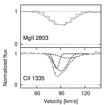
Figure 7.— Upper panel: the Mg II $\lambda$2803 absorption profile of component 3 of image A ($R\sim$10,000). The gray line shows the fitted Voigt profile. Although this velocity component is known to be composed of three sub-velocity components (RSB99), we fitted just one component because the Mg II absorption profile is convolved with the instrumental function of $\sim$30 kms^-1 which is much larger than the intrinsic width ($\sim$10 kms^-1) of the velocity sub-components. Lower panel:the C II $\lambda$1335 absorption profile of component 3 of image A ($R\sim$70,000). The black line shows the observed normalized spectrum from RSB99. The three black dashed lines show the fitted Voigt profiles while the gray line shows the combined profile.

Component 3. Because the influence of the telluric absorption lines is little for component 3 (Figure 4), which is consistent with the doublet ratio of component 3 for image B as discussed above, we fitted a Voigt profile to this component for both Mg II $\lambda\lambda$2796, 2803 lines simultaneously (Table 2). Because the optical absorption profiles are asymmetric for both images A and C (see Figure 5), RSB99 fitted three velocity sub-components to the profile of image A. Because they did not show the fitting results in their paper, we newly fitted the three sub-components to their data (Figure 7) : the fitting results for the three sub-components are $\log N$(C II)[cm^-2]=13.06, 13.49, 12.96, and b=3.5, 9.4, 14.9 km s^-1, respectively. The observed Mg II absorption profile of component 3 is also found to be slightly asymmetric. Although, at first, we tried to fit multi-components to component 3, Mg II absorption lines with the three components identified by RSB99, the resultant fitting uncertainties were very large because of the lower spectral resolution ($\Delta v\sim 30$ km s^-1) compared with the widths of three components ($b<10$ km s^-1). Therefore, we treat component 3 as a single component for both images in the fitting with VPFIT. Although the resultant Doppler width does not have any physical meaning, the estimated column density is expected to be accurate, at least for image B, because the Mg II absorption lines are not saturated for image B as expected from the doublet ratio. For image A, though the Mg II $\lambda$2803 line is expected to be slightly saturated in view of the column density (10¹³ cm^-2) and the expected smallest Doppler width (9 km s^-1), the resultant column density of Mg II is expected to be reasonably accurate.

4.3. Fe II Absorption Lines

Because iron is essential to assess the chemical abundance of the object, the detection of Fe II absorption lines for the $z=3.54$ system is important to understand the nature of this high-$z$ gas cloud. Note that the detection of Fe II $\lambda$1608 in Keck HIRES spectra is not reported so far because the past optical observations of B1422+231 (Rauch et al., 2001a; Songaila & Cowie, 1996) do not cover the wavelength of the shifted Fe II $\lambda$1608 absorption line of $z=3.54$ system ($\sim$ 7300 Å). In our Subaru IRCS spectra, two Fe II lines, $\lambda$2383, $\lambda$2600, with the largest oscillator strengths were detected, but only for component 3 of image A, which has a higher column density for all the $\alpha$-elements.

In order to examine the other velocity components of the Fe II absorption lines for each image A and B, we combined spectra for $\lambda$2344, $\lambda$2383 and $\lambda$2600 lines to improve the S/N for Fe II detection. We did not use $\lambda$2587 for this combining because of the intrinsic weakness and the resultant low S/N. First we transformed the profiles of $\lambda$2344, $\lambda$2383 lines to that of $\lambda$2600 using the following equation:

$$s^{\prime}(\lambda)=1-\left(1-s(\lambda\times\frac{\lambda_{2600}}{\lambda_{2344\ \text{or}\ 2383}})\right)\frac{f_{2600}}{f_{2344\ \text{or}\ 2383}}$$ (4)

where $s(\lambda)$ is the observed spectrum, $s^{\prime}(\lambda)$ is the transformed spectrum, and $f$ is the oscillator strength of the lines. Before the combining, the spectrum for Fe II $\lambda$2600 ($R=$10,000, $\Delta v=30\ \text{km s}^{-1}$) is smoothed to match the spectral resolution to that of $\lambda$2344 and $\lambda$2383 ($R=$5,000, $\Delta v=60\ \text{km s}^{-1}$). Finally each spectrum is combined with weighting by square of the S/N of the continuum around the absorption lines. The resultant spectra are shown at the top of Figure 6. We also plotted the expected absorption lines with gray lines in Figure 6 assuming $\log N$(Mg II)/$N$(Fe II) = 0.31, which is the value for component 3 of image A in Table 2 when we assume that the absorption line is composed of a single velocity component. As a result of Voigt profile fitting for these detected Fe II absorption lines, they are found to have a very large Doppler width ($23\pm 6$ km s^-1, Table 2).

For image A, component 3 is clearly detected again on the combined spectrum, confirming the detection. A weak absorption line is newly noticed between the wavelengths of component 1 and component 2. However, because the center velocity has a large offset from that of the Mg II line, it is hard to confirm the detection at more than a $3\sigma$ level with the present data. Similarly, for image B, two dips near the center velocities of components 1 and 2 are found in the combined spectrum, but the detection is tentative because the expected absorption is much weaker in view of the corresponding weak Mg II absorption lines.

For component 3 of image B, compared to the expected absorption profile shown with gray line in the right panel of Figure 6, the observed combined spectrum is almost flat and the absorption appears to be significantly less than the expected amount. The 3$\sigma$ upper limit is calculated as $\log N=12.1$ for this non-detected component. From this, the column density ratio Mg II to Fe II for the component 3 of image B is estimated to be $>0.5$, which appears to be much larger than that of image A, 0.31. This may suggest a large variance of the column density ratio, $\log N$(Mg II)/$N$(Fe II), even in a small scale of $\sim 8\text{pc}$, which is the projected separation between sightlines A and B at $z=3.54$.

Figure 8.— Velocity profiles of the $z=3.54$ system for images $A$(Mg II, $R=$10,000), $B$(Mg II, $R=$10,000), and $C$(C II from RSB99, $R=$70,000) from bottom to top. The velocity is relative to $z=3.53850$. The vertical dashed lines show the peak velocity of components 2 and 3 of image A. The horizontal dashed lines show the normalized continuum level.

5. Discussion

5.1. Small-scale Structure of Absorbing Gas Cloud at $z=3.54$

By comparing the results for images A and B, considerable differences of the column densities of Mg II absorption lines ($\log(N_{A}/N_{B})\sim$ 0.20$\pm 0.12$ dex and 0.37 $\pm 0.08$ dex for component 2 and component 3, respectively) and considerable velocity shears ($|v_{A}-v_{B}|\sim$ 7.0$\pm 5.8$ km s^-1 and 12.3$\pm 0.8$ km s^-1 at $z=3.53850$ for component 2 and component 3, respectively) are found as shown in Figure 8. Considering the alignment of three images A, B, and C, the differences were as expected from RSB99’s interpretation of their optical spectra of images A and C in that the relations of the column densities and the relative velocities among three images are $\log N_{A}>\log N_{B}>\log N_{C}$ (assuming $\log N(\text{{Mg~{}II}})/N(\text{{C~{}II}})$ is equal for both images B and C ) and $|v_{A}|<|v_{B}|<|v_{C}|$ for both components 2 and 3. The projected distances at $z=3.54$ between images are $d_{AB}=8.4h_{70}^{-1}$ pc and $d_{AC}=22.2h_{70}^{-1}$ pc. This very high spatial resolution (10 pc at $z=3.54$ corresponds to $\sim$ 1 mas angular resolution for direct imaging) shows the power of the gravitational lensing (RSB99).

B1422+231 also has a QSO absorption system at slightly higher redshift (z=3.624) and the transverse distance reaches 1 pc, which is the smallest separation for QSO absorption systems ever studied with gravitationally lensed QSOs (Bechtold & Yee, 1995; Rauch et al., 2001a), though the system shows few variations of absorption lines among multiple images (see Figure 5 of Rauch et al., 2001a) and this system is likely to be associated with the QSO itself. Therefore, the $\sim$ 10 pc structure for the $z=3.54$ system is the smallest spatial structure ever detected for QSO absorption systems.

Ellison et al. (2004) observed three lensed images of gravitationally lensed QSO APM08279+5255(z=3.911) with Hubble Space Telescope (HST). They detected many metal absorption lines at $1.1<z<3.8$, which correspond to the transverse distance, from 30 $h_{70}^{-1}$ pc to 2.7 $h_{70}^{-1}$ kpc. They found large variations of EWs for lower ionization systems, which are traced with Mg II doublet lines, even on the spatial scale of a few hundred pc while the higher ionization systems, which are traced with C IV doublet lines, show less variations of EWs (Rauch et al., 2001a; Ellison et al., 2004). Therefore, low ionization systems should reflect small scale gas clouds, which are likely to be related to star formation activities in galaxies. Because this $z=3.54$ system’s spatial scale ($\sim$ 10 pc) corresponds to that of the typical Galactic gas clouds, such as giant molecular clouds, H II regions, and SNRs (Rauch et al., 1999), the $z=3.54$ system toward B1422+231 is a very precious target that enables the study of such Galactic-scale objects in detail at the galaxy-forming epoch.

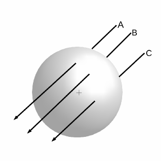
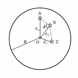
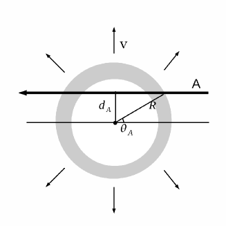
Figure 9.— Images of the expanding shell to illustrate the formulation in the text (Section 5.2.1) for the case where information from three sightlines, A, B, and C, is available. Left panel: the 3D image of sightlines that pass through the shell. Middle panel: the expanding shell seen from the direction of sightlines, showing the definitions of $d_{A},d_{B},d_{C}$, and $\phi$. Right panel: the cross-section of the shell that contains the sightline of image A and the center of the shell, showing the definition of $\theta_{A}$. Similarly, $\theta_{B}$ and $\theta_{C}$ are defined for the sightlines of images B and C, respectively.

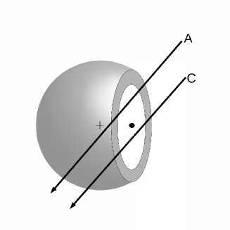
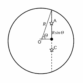
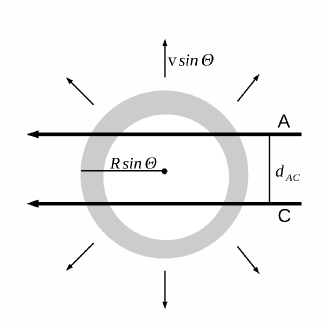
Figure 10.— Images of the expanding shell to illustrate the formulation in the text (Section 5.2.1) for the case where information from two sightlines, A and C, is available. Left panel: the 3D image of sightlines that pass through a circle that is off the center of the shell. Middle panel: the expanding shell seen from the direction of sightlines, showing the definition of $\Theta$. The radius of the cross-section is $R\sin\Theta$. Right panel: the cross-section of the shell that contains the sightlines of images A and C. Though we can constrain $R\sin\Theta$ and $v\sin\Theta$, we cannot infer the radius $R$ and expansion velocity $v$ due to the lack of information of another independent sightline, such as the sightline B.

5.2. Expanding SNR Shell

5.2.1 Shell Model

The column densities and the velocities of Mg II absorption lines of components 2 and 3 vary among three sightlines as $\log N_{A}>\log N_{B}>\log N_{C}$ and $|v_{A}|<|v_{B}|<|v_{C}|$. What types of object can generate these systematic variances on such a small scale? Based on the nearly symmetric velocity profiles of components 2 and 3 with respect to the systemic velocity that corresponds to $z=3.53850$ that are seen in optical spectra of both images A and B (see the profiles for C II and Si II in Figure 5), RSB99 suggested that the components 2 and 3 of the $z=3.54$ system can be an expanding shell, such as an SNR. When the sightline passes through the center of a gas cloud of the expanding shell, the observed velocity becomes highest because the gas expands along the direction of the sightline while the column density becomes lowest because the path of the sightline in the shell is shortest at the center. On the other hand, when the sightline passes through the outer edge, the observed velocity becomes lowest, while the column density becomes highest. Applying this model to the $z=3.54$ system, RSB99 found that the sightlines of images A and C pass near the outer edge and near the center of an expanding gaseous shell, respectively. The absorption lines of image B, which is newly observed in this study, shows intermediate values for both column density and relative velocity; this systematic kinematics seen in this gas cloud support the idea of RSB99 that this $z=3.54$ system is truly an expanding shell. Although a contracting (or collapsing) shell is an alternative choice, such an astronomical object is unlikely because the central object of the shell has to pull all the gas symmetrically in a subtle manner: normally such gas should fall through a disk or infalling envelope (not a shell). In fact, no such object is known in the Galaxy and near-by galaxies (see the listed examples of astronomical objects in Section 5.2 in Rauch et al. 2002).

Following RSB99 and Rauch et al. (2002), we will consider a model of a three-dimensional (3D) expanding shell (Figure 9) that has a radius of $R$ and an expansion velocity of $v_{\text{exp}}$. Those parameters can be constrained by two kinds of observables: the physical distance between two sightlines at the redshift (e.g., $d_{AB}$) and the velocity difference of the two absorption components seen in a single sightline (e.g., $\Delta v_{A}$). In case only two sightlines are available, only the parameters for the expansion “ring” that is on the plane of the two sightlines can be constrained: one is the radius of the ring ($R\sin\Theta$) and the other is the expansion velocity of the ring ($v_{\text{exp}}\sin\Theta$), where $\Theta$ is the declination of the ring on the sphere (Figure 10). Although the relation between $R\sin\Theta$ and $v_{\text{exp}}\sin\Theta$ can be obtained, the 3D radius ($R$) and the expansion velocity ($v_{\text{exp}}$) can never be determined because of the complete lack of the information on the absolute location of the ring ($\Theta$) on the sphere: only the possible range of $R\sin\Theta$ and the lower-limit of $v_{\text{exp}}\sin\Theta$ can be obtained (RSB99).

On the other hand, in case three independent sightlines (not on a single plane) are available, we can put a strong constraint on the expanding sphere. Since the absolute location of the planes that contain the sightlines cannot be determined in a unique way, $R$ and $v_{\text{exp}}$ still cannot be determined. However, if the $R$ value is fixed, the other parameter $v_{\text{exp}}$ is determined because two $\Theta$s for the sets of two sightlines (e.g., A/B and B/C) can be determined from the two equations for two rings. Therefore, the relation between $R$ and $v_{\text{exp}}$, which is useful to elucidate the astronomical nature of the shell, can be obtained as a final product (see the detailed description in Appendix of Rauch et al. 2002). In fact, Rauch et al. (2002) suggested that the $z=0.5656$ absorption system in the three sightlines of gravitationally lensed QSO Q2237+0305 is also an expanding shell because the absorption lines showed variances similar to those of the $z=3.54$ system. They analysed the relation between the radius and expansion velocity of the 3D shell and concluded that the expanding shell at $z=0.5656$ can be interpreted as a supershell or a superbubble of 1-2 kpc size that is frequently observed in the Galaxy and extra-galaxies.

Based on the radial velocities in the two lines of sight (images A and C), RSB99 managed to constrain the parameters in a ring for the $z=3.54$ system as 9 $h_{70}^{-1}<R\sin\Theta<$ 34 $h_{70}^{-1}$ pc and $v_{\text{exp}}\sin\Theta>98\ \text{km s}^{-1}$. Now, with the additional information of image B, we can obtain the relation of $R$ and $v_{\text{exp}}$ of the expanding shell at $z=3.54$. Note that the model parameters can be completely determined if we have four independent sightlines. Because B1422+231 has four independent gravitationally lensed images, future observations of the fourth image would be very valuable.

We formulated the geometry of the expanding shell as shown in Figure 9 to obtain the radius-velocity relation of the $z=3.54$ system. The difference of velocities of components 2 and 3 in the sightline of image A, $(\Delta v)_{A}$, and the distance from the center of the shell to the sightline A, $d_{A}$, can be expressed as

$$(\Delta v)_{A}=2v_{\text{exp}}\cos\theta_{A}$$ (5)

$$d_{A}=R\sin\theta_{A},$$ (6)

where $\theta_{A}$ is the angle from the center of the shell to the sightline A (see Figure 9). The equations for images B and C can be given similarly, resulting in six equations in total. Next, we can derive two equations about the geometry of triangle ABC :

$$d_{A}^{2}=d_{B}^{2}+\overline{AB}^{2}+2d_{B}\overline{AB}\cos{\phi}$$ (7)

$$d_{C}^{2}=d_{B}^{2}+\overline{BC}^{2}+2d_{B}\overline{BC}\cos{[\angle ABC-\phi]},$$ (8)

where $\overline{AB}$ and $\overline{BC}$ are projected distances between images at $z=3.54$, $\phi$ is the angle between BA and BO, and $\angle ABC$ is the angle between BA and BC. Now, the parameters $(\Delta v)_{A}$, $(\Delta v)_{B}$, $(\Delta v)_{C}$, $\overline{AB}$, $\overline{BC}$, $\angle ABC$, are observed and the nine parameters $R$, $v_{\text{exp}}$, $d_{A}$, $d_{B}$, $d_{C}$, $\theta_{A}$, $\theta_{B}$, $\theta_{C}$, $\phi$ are not determined. If these eight equations are combined, the $R(v_{\text{exp}})$ relation can be obtained as a solution.

For the $z=3.54$ system, the projected distances are $\overline{AB}=8.4h_{70}^{-1}$ pc, $\overline{BC}=14.4h_{70}^{-1}$ pc, and $\overline{AC}=22.2h_{70}^{-1}$ pc at $z=3.54$. The angle between AB and BC is 153^∘. The velocity differences between components 2 and 3 are $(\Delta v)_{A}=168\pm 1$ km s^-1, $(\Delta v)_{B}=188\pm 3$ km s^-1, and $(\Delta v)_{C}=197\pm 1$ km s^-1. By putting those values into the equations, we obtained the function $R(v_{\text{exp}})$ that is shown with a solid line in Figure 11 along with two dashed lines that show the 1$\sigma$ uncertainty range of our calculation : each line corresponds to the cases of $(\Delta v)_{B}=$ 185 km s^-1, 191 km s^-1. Here, we are only concerned with the uncertainty of $(\Delta v)_{B}$ because it is the largest among six observables : the available spectrum of image B is only our lower-resolution near-infrared data while the available spectra of the other two images A and C are higher-resolution optical data of RSB99.

Figure 11.— Relation of radius and expansion velocity of the expanding shell model. The solid line shows the relation for the $z=3.54$ system in the case of $(\Delta v)_{B}=188$ km s^-1, which is the most likely value from the observation (see Section 5.2.1 for detail). The dotted lines along the solid line are the case of $(\Delta v)_{B}=185,191$ km s^-1, showing 1$\sigma$ uncertainty of our calculation. The filled and open circles show the radius and expansion velocity of the observed SNRs and H II regions in our Galaxy (Koo & Heiles, 1991; Shields, 1990; Kothes & Kerton, 2002; Arnal & Corti, 2007; Daigle et al., 2007; Cappa et al., 2008; Cichowolski et al., 2008).

5.2.2 The SNR Origin of the Shell

Figure 11 shows that the radius of the shell is larger than $\sim 20$ pc and the expansion velocity is larger than $\sim 120$ km s^-1. Although there is no a priori constraints, the shortest radius ($R\leq 30$ pc) is unlikely because it requires: (1) an exact alignment of the shell with the three sightlines that have similar separations as the shell diameter and (2) very high velocity ($v_{\text{exp}}>200$ km s^-1) that appears to be too fast for an H I shell. The largest radius ($R\gg 100$ pc) is also unlikely since it requires similarly very high expansion velocity and all three sightlines must pass near the edge of expanding shell, exactly. Therefore, the bottom of the curve ($R\sim 50-100$ pc, $v_{\text{exp}}\sim 130$ km s^-1) would be the natural choice of the radius and the expansion velocity of the shell (see the original discussion in Rauch et al. 2002 for another QSO absorption system).

To compare to the known astronomical shell-like objects, we also plotted the radii and expansion velocities observed for the Galactic H II regions (Shields 1990; Kothes & Kerton 2002; Arnal & Corti 2007; Daigle et al. 2007; Cappa et al. 2008; Cichowolski et al. 2008) and SNRs that have a structure of expanding shell: the data points of SNR are from Koo & Heiles (1991), who observed 15 old SNRs with H I 21cm line in the disk of our Galaxy. As a result, the location of the $z=3.54$ system on the plot is found to be quite consistent with SNRs while all the H II regions show much smaller expansion velocity less than 20 km s^-1. In fact, the distributions of SNRs match well with the bottom of the curve for the $z=3.54$ system, which is quite consistent with the above consideration that the bottom of the curve is the most likely location of the shell. Therefore, we concluded that the shell is truly an SNR shell, confirming RSB99’s initial suggestion in more solid way.

5.2.3 Physical Parameters of the SNR Shell

Assuming $R=50-100$ pc and $v_{\text{exp}}=130$ km s^-1 as the radius and the expansion velocity of the observed shell, we compare the observed SNR shell with the typical self-similar expansion model to estimate the main physical parameters of the shell. Then, we compare the estimated physical parameters to those of typical SNRs to check the consistency of the SNR interpretation. In the following, we will utilize the formulation described in text-books by Tielens (2005) and Draine (2011) to first estimate the age ($t$) of the SNR shell, and finally the total energy ($E$) of the shell, along with an independent estimate of mass ($M$) of the shell from the column densities of the absorption lines.

If the self-similar concept is introduced with a simple power laws ($R\propto t^{\eta}$), the age of the shell can be roughly estimated from $R$ and $v_{\text{exp}}$ as $t\sim 10^{5}$yr for $z=3.54$ system since $t\sim R/v_{\text{exp}}$. The SNR shell of this age is in the radiative expansion phase (snowplow phase) rather than adiabatic expansion phase (Sedov phase). In this case, $\eta=2/7$ and the age $t$ can be derived with

$$t=1.1\times 10^{5}\text{yr}\left(\frac{R}{50\text{pc}}\right)\left(\frac{v_{\text{exp}}}{130\text{km s}^{-1}}\right)^{-1}.$$ (9)

For the observed $v_{\text{exp}}$ (130 km s^-1) and the range of $R$ (50 - 100 pc), the age of the $z=3.54$ shell is estimated as:

$$1.1\times 10^{5}\text{yr}\leq t\leq 2.2\times 10^{5}\text{yr}.$$ (10)

In this snowplow phase, the radius and expansion velocity are modeled as

$$R(t)=21.6\text{pc}\left(\frac{E_{0}}{10^{51}\text{erg}}\right)^{\frac{11}{45}}\left(\frac{n_{0}}{1\text{cm}^{-3}}\right)^{-\frac{11}{45}}\left(\frac{v_{\text{exp}}(t)}{250\,\text{km s${}^{-1}$}}\right)^{-\frac{2}{5}},$$ (11)

where $E_{0}$ is the total energy of a supernova, $n_{0}$ is the number density of the interstellar gas before the supernova explosion.

Next, we will discuss the mass of the shell ($M_{\text{tot}}$). RSB99 estimated the number density ($n$) and the size along the line of sight ($L$) for the component 3 of image A using photoionization model as

$$0.16\text{ cm}^{-3}\leq n\leq 1.6\text{ cm}^{-3}$$ (12)

$$0.015\text{ pc}\leq L\leq 1.6\text{ pc}.$$ (13)

From these parameters, RSB99 estimated the mass of a gas cloud ($M_{\text{tot}}$) assuming two geometrical cases ; first is a homogeneous cylindrical slab with a thickness $L$ and radius $\overline{AC}$ as a lower limit of the mass; second is a spherical cloud with a radius $\overline{AC}$ as an upper limit of the mass:

$$0.4M_{\odot}\leq M_{\text{tot}}\leq 2700M_{\odot}.$$ (14)

Here, we newly obtained an additional constraint on the radius $R$ of the gas cloud as $R\sim 50-100$ pc. Assuming that the gas cloud has a shape of spherical shell with an average radius of $R$, thickness of $L$, and number density of $n$, we can calculate the total mass $M_{\text{tot}}$ of the shell with

$$M_{\text{tot}}=4\pi R^{2}Lnm_{\text{{H~{}I}}}\mu,$$ (15)

where $m_{\text{{H~{}I}}}$ is the mass of a hydrogen atom particle ($m_{\text{{H~{}I}}}=1.66\times 10^{-24}$g) and $\mu$ is the reduced mass ($\mu=4/3$). Here we ignored the effect of $\cos\theta_{A}$ on the thickness of the shell (see Figure 9) in view of the large uncertainty of $L$. Using the value range of $n$ and $L$ (Equation 12 and 13) and our result on the radius ($50<R<100\ \text{pc}$), $M_{\text{tot}}$ is estimated as:

$$25M_{\odot}\leq M_{\text{tot}}\leq 1050M_{\odot}.$$ (16)

This is consistent with the original mass estimate by RSB99 (Equation 14), but narrows the mass range by two orders of magnitude.

Because the uncertainty of this estimate is quite large, we try an alternative mass estimate in the following. We will estimate the mass in two ways here, using the column density of H I or Mg II, in order to check the consistency. In both estimates, we will use the column density of component 3 of image A because the ionization parameter, $\log U$, of this component was specifically estimated as $\log U=-4.4$ (RSB99) which is low enough that we can estimate the mass simply from observed column density without any ionization correction. Although the column density of this component may not be the representative value of the shell, we would not expect a large uncertainty of more than an order of magnitude in view of the column density variation among the components seen in images A, B and C.

First, the H I mass of the shell can be simply calculated as :

$$M_{\text{{H~{}I}}}=4\pi R^{2}N_{\text{{H~{}I}}}m_{\text{{H~{}I}}}$$ (17)

where $R$ is the size of the shell and $N_{\text{{H~{}I}}}$ is the observed H I column density. Using $\log N$(H I)=$16.05\pm 0.15$ for component 3 of image A (RSB99), the H I mass is calculated as

$$2.8M_{\odot}\leq M_{\text{{H~{}I}}}\leq 11M_{\odot}$$ (18)

Because this gas cloud is optically thin, almost all of the hydrogen is likely to be ionized. To estimate the total mass of the shell from the H I mass, we must evaluate the degree of ionization. In Donahue & Shull (1991), the fraction of H I is calculated with

$$\frac{n(\text{{H~{}I}})}{n_{H}}=(4.6\times 10^{-6})U^{-1.026},-4.7<\log U<-1.8,$$ (19)

where $n$(H I) is the number density of only H I and $n_{\text{H}}$ is the total number density of hydrogen atom that includes H II. Since the ionization parameter of the component 3 of image A is estimated as $\log U=-4.4$ (RSB99), $n(\text{{H~{}I}})/n(\text{H})$ is calculated as 0.15. Then, the total hydrogen mass is estimated as:

$$19M_{\odot}\leq M_{H}\leq 75M_{\odot}.$$ (20)

Finally, the total mass of the shell can be calculated by multiplying the reduced mass, $\mu$, as:

$$25M_{\odot}\leq M_{\text{tot}}\leq 99M_{\odot}.$$ (21)

This range is consistent with the typical scrambled gas mass of the observed SNR (10 - 1000 $M_{\odot}$), with a radius from about 10 to a few 100 pc (Koo & Heiles, 1991).

Next, we attempt one more independent estimate of the total mass of the shell based on the column density of Mg II instead of H I. The total Mg II mass in the shell can be estimated using Equation (17) but after replacing H I to Mg II. For column density $N_{\text{{Mg~{}II}}}$, we use the value of component 3 of image A because this component is examined in detail by RSB99. As a result, the total Mg II mass is calculated as

$$0.06M_{\odot}<M_{\text{{Mg~{}II}}}<0.24M_{\odot}$$ (22)

for the assumed range of radius.

The total mass of the shell can be estimated first assuming that all the magnesium is in the form of Mg II. This assumption is reasonable because the Mg I absorption lines are not detected (the 3$\sigma$ upper limit is calculated as $\log N(\text{{Mg~{}I}})[\text{cm}^{-2}]<11.1$; see Section 4.1 or Table 2. Although the possibility of the existence of a significant amount of Mg III cannot be dismissed, we ignored the higher ionization states because the ionization parameter $\log U$ of this component is estimated to be quite low as $\log U=-4.4$ (RSB99) based on the photoionization modeling of Donahue & Shull (1991). We assumed the solar abundance, which is suggested by RSB99 for component 3 based on the photoionization modeling by Donahue & Shull (1991). With the solar abundance of magnesium (0.13% in mass; Grevesse et al., 2010), the total mass $M_{\text{tot}}$ is estimated from Equation (22) as

$$47M_{\odot}<M_{\text{tot}}<188M_{\odot}.$$ (23)

This mass range is pretty much consistent with the estimate from H I column density, Equation (21).

From the estimated radius and expansion velocity, we can finally constrain the energy of supernova explosion using Equation (11). The remaining parameter in this equation, $n_{0}$, which is the number density of interstellar medium around the supernova before explosion, can be estimated assuming that the shell consists of all of the gas that existed in the sphere with radius $R$ before explosion, with the following equation:

$$n_{0}=\frac{3M_{\text{tot}}}{4\pi R^{3}m_{H}\mu}.$$ (24)

With the range of $50\leq R\leq 100\text{ pc}$ and $M_{\text{tot}}$ from Equation (23), $n_{0}$ is calculated as:

$$1.8\times 10^{-3}\text{cm}^{-3}<n_{0}<3.6\times 10^{-3}\text{cm}^{-3}$$ (25)

Then, the energy of supernova explosion, $E_{0}$, is calculated with Equation (11):

$$3.8\times 10^{49}\text{erg}<E_{0}<3.2\times 10^{50}\text{erg}$$ (26)

The estimated energy is roughly consistent with the energy of supernova explosion, $\sim 10^{51}$ erg (Tielens, 2005; Draine, 2011). The slight difference can be attributed to the left-over gas inside the shell (see e.g., Koo & Heiles, 1991) that can effectively increase $n_{0}$, thus $E_{0}$ through Equation (11).

In this subsection, we have gone through the physical parameters of the $z=3.54$ system as an expanding shell of an SNR. The expanding shell model and estimated physical parameters appear to be quite consistent with the properties of SNRs observed in the galaxy. With our calculation, this system is likely to be an SNR of about 0.1 Myr with a radius of 50 $-$ 100 pc, an expansion velocity of about 130 km s^-1, and the total energy of $10^{50}$ erg. Therefore, we conclude that this $z=3.54$ system is truly an SNR.

Figure 12.— $N$(Mg II) vs. $N$(Mg II)/$N$(Fe II) of weak Mg II systems. The crosses are from Narayanan et al. (2008), the squares are from Rigby et al. (2002), and a filled circle shows the component 3 of image A of the $z=3.54$ system. The filled squares show confirmed Fe-rich systems while a open square shows confirmed non Fe-rich system (Rigby et al., 2002). The dotted line shows the solar abundance ratio (Asplund et al., 2005). The $z=3.54$ system (filled circle) is located in a horizontal branch near the solar value, where the confirmed Fe-rich systems (filled squares) are distributed.

5.3. Type Ia Supernova ?

Recall the very broad profile of Fe II absorption lines of component 3 in image A, which is described in Section 4.2. What does this feature mean in the SNR interpretation of the $z=3.54$ system? To answer this question, we first discuss the iron richness of the SNR shell, then examine the broad absorption feature in a more rigorous way to suggest that the iron is localized in the SNR shell. Finally, we conclude that the SNR shell is related to an SN Ia.

5.3.1 Fe Richness

The amount of iron in the gas cloud is crucial to investigate the chemical enrichment by supernovae. Figure 12 shows the distribution of $\log N(\text{{Mg~{}II}})/N(\text{{Fe~{}II}})$ versus $\log N$(Mg II) for weak Mg II systems. The crosses are from Narayanan et al. (2008), who studied 100 weak Mg II systems at $0.4<z<2.4$ using VLT data. The four squares are weak Mg II systems studied with Keck data by Rigby et al. (2002). Note that neither sample includes the systems whose Fe II are not detected. The filled and open squares are confirmed Fe-rich and non-Fe-rich systems based on their photoionization modeling using CLOUDY, respectively. The filled circle shows the $z=3.54$ system ($\log N(\text{{Mg~{}II}})/N(\text{{Fe~{}II}})$=0.31$\pm$0.07). The dotted line shows the solar abundance ratio, $\log[N(\text{Mg})/N(\text{Fe})]_{\odot}$ = 0.08 (Asplund et al., 2005) for the case that all Mg and Fe atoms are in the Mg II and Fe II ionization states. The value of the $z=3.54$ system is found to be closer to the solar value than those for the other weak Mg II systems with similar $N$(Mg II). Narayanan et al. (2008) suggested that any system near the solar value (dashed line in Figure 12) are truly Fe-rich systems.

Rigby et al. (2002) suggested that their three Fe-rich systems ($N$(Fe II)$\sim$$N$(Mg II)) have small sizes of $\sim 10$pc, and high metallicity of $>0.1Z_{\odot}$ (see filled squares in Figure 12). They specifically predicted that the $z=3.54$ system toward B1422+231 should show strong Fe II lines ($N$(Fe II) $\sim$ $N$(Mg II)) in view of the small spatial structure ($\sim$10 pc) and high metallicity inferred by RSB99. In fact, $\log N(\text{{Mg~{}II}})/N(\text{{Fe~{}II}})$ of the $z=3.54$ system is found to be similarly Fe-rich as the three Fe-rich systems (see Figure 12), suggesting solar to sub-solar metallicity.

All those results support the iron-richness of the SNR shell at $z=3.54$. The high iron abundance of the SNR naturally suggests that it is an SN Ia. In fact, Rigby et al. (2002) suggested that the three iron-rich systems in their samples have [$\alpha$/Fe]$<0$ and have been enriched by SNe Ia because high iron column density that is similar to magnesium column density cannot be explained by other enrichment processes such as SNe II. Therefore, it is highly likely that the $z=3.54$ system is a gas cloud enriched by SNe Ia. More detailed arguments based on abundance estimate using CLOUDY photoionization modeling will be presented in our separate paper (S. Kondo et al. in preparation).

If the gas cloud was truly enriched by SNIa explosion, the total amount of the iron in the gas should be consistent with the yield of the iron from SNIa explosion. Assuming the Fe II absorbing gas is in the form of shell with $R=50-100$ pc as Equation (17), the Fe II mass is estimated as 0.07-0.29 $M_{\odot}$ from the component 3 of image A. Our estimated Fe II mass is consistent with the observed mass of SNeIa. Scalzo et al. (2010) and Silverman et al. (2011) suggest that the estimated mass of radio active ⁵⁶Ni (eventually decays to ⁵⁶Fe) ejected from an SN Ia ranges from 0.02 $M_{\odot}$ to 1.7 $M_{\odot}$. Note that the slightly low estimated energy of the SN (Section 5.2.3) also favors an SNIa interpretation rather than other types of SN with more energetic explosions. Because our estimate does not include the iron in other ionization states, such as Fe III, within the shell as well as the iron inside the shell, the total mass of iron is expected to be more than the estimated value.

5.3.2 Fe Localization

Another characteristic of the Fe II absorption line is the Doppler width ($23\pm 6$ km s^-1) that appears to be unusually broad compared with that of $\alpha$-element (e.g., $b_{\text{{Mg~{}II}}}\sim 9$ km s^-1). This is quite strange for a QSO absorption system, because the mass of an iron atom is much heavier than that of $\alpha$ elements, thus the width of an Fe II absorption line should be smaller than that of $\alpha$ elements. We first compared the widths of Mg II and Fe II lines of the $z=3.54$ system with the past surveys of weak Mg II systems (Rigby et al., 2002; Churchill et al., 2003b; Narayanan et al., 2008). Figure 13 shows correlation of the Doppler widths of Mg II and Fe II lines of weak Mg II systems. The points should be located below the dotted line ($b_{\text{{Mg~{}II}}}=b_{\text{{Fe~{}II}}}$) because iron is heavier than magnesium. In fact, most data points from the literatures are distributed along or below the dotted line. However, the $z=3.54$ system is found to be located significantly above the line even considering the uncertainty, suggesting the uniqueness of this system.

We first checked the possibility of blending of other absorption lines on the Fe II absorption lines. For example, if Mg II absorption systems existed at $z=$3.22 and $z=$2.87, strong metal absorption lines Mg II $\lambda\lambda$2796, 2803 would blend with the Fe II $\lambda$2600 ($\lambda=11804$ Å) and $\lambda$2383 ($\lambda=10814$Å) lines, respectively. However, such absorption systems have not been reported in Songaila & Cowie (1996) and Rauch et al. (2001a), who detected many Lyman series lines and C IV absorption lines of B1422+231. Therefore, we conclude that the broad features of Fe II lines are real.

Here we try to evaluate the excess Fe II absorption by decoupling the broad feature into two sub-components. If we compare the Mg II and Fe II profiles, the excess exists on the blue side of the Mg II absorption peak (Figure 6). Then, we fitted two velocity components to both Fe II $\lambda$2600 and $\lambda$2383 lines with the fixed Doppler widths of 9 km s^-1 , which is the upper limit estimated from the Doppler width of Mg II ($\sim 9$ km s^-1). The results are shown in the bottom panel of Figure 14. The black line shows the component whose redshift is fixed to the value of the Mg II absorption line during the fitting, while the gray line shows the other excess component, for which the redshift was not fixed. The resultant difference of peak velocity between the two velocity components is $26\pm 7$ km s^-1, and the column densities of blue and red components are $\log N$ [cm^-2] = $12.3\pm 0.2$ and $12.5\pm 0.1$, respectively. This fitting appears to match well with the observed data for both Fe II $\lambda$2600 and $\lambda$2383 lines.

Now, the question is what is the blue component ? Because there is no obviously corresponding $\alpha$-element absorption lines, this iron gas cloud is inferred to be localized in the shell. The localization of iron in the SNR also supports the SNIa origin of the SNR shell: the Fe II features imply the ejection of the mass from the SN Ia, while the other $\alpha$-element absorption lines are likely to be the interstellar gas scrambled by the shock of the SNR. In our Galaxy, Hamilton et al. (1997) observed SN1006, which is an SN Ia remnant, with absorption lines on a spectrum of Schweizer and Middleditch star, whose sightline intersects near the center of SN1006. Despite the age difference ($\sim$1000 yr for SN1006, $\sim 10^{5}$ yr for the $z=3.54$ system), it would be useful to compare those two objects in detail to infer the nature of the $z=3.54$ SNR shell because the geometrical configuration is very similar. For SN1006, very broad ($\sim$ 5,000 km s^-1) Fe II absorption line is detected at the systemic velocity while the ejected Si II shows a redshift of $\sim$ 5,000 km s^-1. This suggests that the mixing of ejected iron with interstellar gas occurs after the mixing of ejected $\alpha$-elements. The two velocity sub-components of Fe II absorption lines of component 3 of image A can be interpreted as meaning that the red component with the same velocity as the $\alpha$-element lines comes from Fe gas that mixed with the scrambled interstellar gas, and the blue component comes from Fe gas that has not been mixed with it yet (Figure 15). Therefore, we might witness the mixing process of ejected iron with interstellar gas at $z=3.54$.

Figure 13.— Correlation of Doppler widths of Mg II and Fe II absorption lines of weak Mg II systems. The crosses are from Rigby et al. (2002), Churchill et al. (2003b), Narayanan et al. (2008), while the filled circle shows the $z=3.54$ system (component 3 of image A). The dotted line shows the location where the widths of Mg II and Fe II are identical. While the crosses are distributed along or below the dotted line, the point of the $z=3.54$ system is located above the line with a large offset.

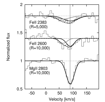
Figure 14.— Voigt profile fitting to the Mg II $\lambda$2803 (bottom), Fe II $\lambda$2600 (middle) and $\lambda$2383 (top) absorption lines of component 3 of image A. The thin lines show the observed spectra. The solid thick lines show the fitted Voigt profiles with the Doppler width and redshift fixed to the values of Mg II absorption lines. The gray lines show the fitted Voigt profiles to the residual absorption. The dashed lines show the combined profiles of black and gray components.

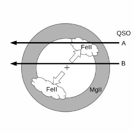
Figure 15.— Schematic image of the SNR shell of the $z=3.54$ system. The Fe-rich gas clouds are localized in the expanding shell, while the $\alpha$ element gas clouds, such as Mg II, are distributed homogenously in the expanding shell.

5.3.3 SNe Ia at High Redshift

In this section, we saw the evidence of the richness and localization of iron in the SNR shell at $z=3.54$. The detected iron richness cannot be explained by processes other than SN Ia. Moreover, the suggested localization of iron in the shell supports the SN Ia interpretation. From these facts, we conclude that the $z=3.54$ system is an SN Ia remnant.

The extragalactic SN Ia has been studied extensively for the supernova cosmology (Goobar & Leibundgut, 2011). However, even the most distant SN Ia event ever detected is at $z=1.55$ (Rodney et al., 2012) and more distant objects that are important for the study of cosmic chemical enrichment history are hard to detect and with 8-10 m class telescopes. For studying such high-$z$ SNe Ia, absorption systems toward gravitational-lensed QSO may serve as good targets as is the case for this $z=3.54$ system toward B1422+231. Even for the single sightline, the Fe-rich absorption systems as seen in Figure 12 would become good targets for studying chemical enrichment history at high-redshift ($z>2$) with more data available with sensitive high-resolution spectroscopy with adaptive optics (see Kobayashi et al., 2005).

6. Summary

We obtained near-infrared high-resolution ($R=$10,000) spectra of images A and B of gravitationally lensed QSO B1422+231 with the Subaru 8.2 m telescope and the IRCS echelle spectrograph. Although the observed PSFs of images A and B are partially overlapping in the slit, we managed to extract spectra for each image A and B to examine the differences of absorption lines. We detected Mg II $\lambda\lambda$2796, 2803 absorption lines of the $z=3.54$ system, which had been found in images A and C in optical spectra by RSB99. Corresponding Fe II $\lambda$2383, $\lambda$2600 absorption lines are also detected but only for the component 3 of image A. The projected separation between A and B images at $z=3.54$ is just $8.4h_{70}^{-1}$ pc and we found considerable differences of column density ($\Delta(\log N)\sim 0.3$ dex) and velocity shear ($\Delta v\sim 10$ kms^-1) between both images on such a small scale. These differences suggest the smallest structure of gas clouds ever detected for QSO absorption systems.

Considering the physical origin of the differences of $\alpha$-elements absorption lines among three images A, B, and C, we conclude that the $z=3.54$ system is an expanding shell as originally suggested by RSB99. The information of three images enable us to analyse the 3D structure of the absorbing gas cloud and concluded that this $z=3.54$ system is an SNR shell whose radius and expansion velocity are 50$-$100 pc and $\sim$ 130 km s^-1, respectively. We estimated several physical parameters of the shell, which are found to be consistent with SNRs: the age is $\sim 10^{5}$ yr, the mass of the shell is $\sim$ 100 $M_{\odot}$, and the energy of the SNe is $\sim 10^{50}$ erg.

We also found that the Fe II absorption lines of $z=3.54$ system have much larger column density and Doppler width than those of the weak Mg II systems in the literature. The small column density ratio $\log N$(Mg II)/$N$(Fe II) (=0.31$\pm$0.07) is indicative of the richness of the iron of the $z=3.54$ system. We also estimated the mass of Fe II as 0.07$-$0.29 $M_{\odot}$ which is roughly consistent with the yield of observed SNe Ia. Moreover, the large Doppler width of Fe II, which is interpreted as the existence of one more velocity component that is blueshifted and extremely Fe-rich, suggests that the Fe-rich gas cloud is localized in the expanding shell of SNR. From these results, we conclude that the SNR shell at $z=3.54$ is produced by an SN Ia explosion.

Supernova explosions are thought to be one of the most important processes that drive the formation of galaxy through the dynamical energy input and the chemical enrichment. If this $z=3.54$ system is truly an SNR, it is the farthest sample of a supernova ever observed. If higher S/N and/or higher spectral resolution data of B1422+231 were obtained in the future, the difference between iron and $\alpha$-elements would be more clearly confirmed. Then, physics of the mixing of interstellar gas with ejected gas from supernovae could be discussed in detail. If the spectrum of image D is also obtained, the radius and expansion velocity can be strictly determined with the expanding shell model.

This $z=3.54$ system illustrates the power of the gravitational lensing effect for the study of QSO absorption systems with the extremely high spatial resolution and multiple sightlines. In the case of present study, the separation between images A and B is only $<$ 10 pc at z=3.5 that corresponds to about 1 mas angular resolution. More observations of gravitationally lensed QSOs will reveal the kinematics (e.g., expansion) of gas clouds on interstellar scales at high redshift during crucial phases of galaxy formation.

We are grateful to all of the IRCS and AO team members and the Subaru Telescope observing staffs for their efforts, which made it possible to obtain these data. We are grateful to Dr. Rauch for kindly providing us their B1422+231 optical spectra obtained with Keck/HIRES. This work was supported by KAKENHI Grant-in-Aid for Scientific Research(B) (No. 20340042; N. Kobayashi) from JSPS, and in part by the Graduate University for Advanced Studies (Sokendai). This research has been partially supported by the Private University Strategic Research Foundation Support Program of the Ministry of Education, Science, Sports and Culture of Japan, S0801061.

References

- Arnal & Corti (2007) Arnal, E. M., & Corti, M. 2007, A&A, 476, 255
- Asplund et al. (2005) Asplund, M., Grevesse, N., & Sauval, A. J. 2005, in ASP Conf. Ser. 336. Cosmic Abundances as Records of Stellar Evolution and Nucleosynthesis, ed: T. G. Barnes III & F. N. Bash (San Francisco, CA: ASP), 25
- Bechtold & Yee (1995) Bechtold, J., & Yee, H. K. C. 1995, AJ, 110, 1984
- Cappa et al. (2008) Cappa, C., Niemela, V. S., Amorín, R., & Vasquez, J. 2008, A&A, 477, 173
- Carswell et al. (1987) Carswell, R. F., Ibb, J. K., Baldwin, J. A., & Atwood, B. 1987, ApJ,319, 709
- Churchill et al. (2003a) Churchill, C. W., Mellon, R. R., Charlton, J. C., & Vogt, S. S. 2003, ApJ, 593, 203
- Churchill et al. (1999) Churchill, C. W., Rigby, J. R., Charlton, J. C., & Vogt, S. S. 1999, ApJS, 120, 51
- Churchill et al. (2003b) Churchill, W. C., Vogt, S. S., & Charlton, C. J., 2003b, AJ, 125, 98
- Cichowolski et al. (2008) Cichowolski, S., Romero, G. A., Ortega, M. E., Cappa, C. E., & Vasquez, J. 2008, Boletin de la Asociacion Argentina de Astronomia La Plata Argentina, 51, 185
- Daigle et al. (2007) Daigle, A., Joncas, G., & Parizeau, M. 2007, ApJ, 661, 285
- Donahue & Shull (1991) Donahue, M., & Shull, J. M. 1991, ApJ, 383, 511
- Draine (2011) Draine, B. T. 2011, Physics of the Interstellar and Intergalactic Medium ( Princeton, NJ: Princeton Univ. Press)
- Ellison et al. (2004) Ellison, S. L., Ibata, R., Pettini, M., et al. 2004, A&A, 441, 79
- Ferland et al. (1998) Ferland, G. J., Korista, K. T., Verner, D. A., et al. 1998, PASP, 110, 761
- Foltz et al. (1984) Foltz, C. B., Weymann, R. J., Roser, H.-J., & Chaffee, F. H., Jr. 1984, ApJ, 281, L1
- Grevesse et al. (2010) Grevesse, N., Asplund, M., Sauval, A. J., & Scott, P. 2010, Ap&SS, 328, 179
- Goobar & Leibundgut (2011) Goobar, A., & Leibundgut, B. 2011, Ann. Rev. Nucl. Part. Sci., 61, 251
- Hamilton et al. (1997) Hamilton, A. J. S., Fesen, R. A., Wu, C.-C., Crenshaw, D. M., & Sarazin, C. L. 1997, ApJ, 481, 838
- Iye et al. (2004) Iye, M., Karoji, H., Ando, H., et al. 2004, PASJ, 56, 381.
- Kobayashi et al. (2000) Kobayashi, N., Tokunaga, A. T., Terada, H., et al. 2000, Proc. SPIE, 4008, 1056
- Kobayashi et al. (2002) Kobayashi, N., Terada, H., Goto, M., & Tokunaga, A. 2002, ApJ, 569, 676
- Kobayashi et al. (2005) Kobayashi, N., Tsujimoto, T., & Minowa, Y. 2005, in Science with Adaptive Optics, ed. W. Brandner & M. E. Kasper (Berlin: Springer), 352
- Koo & Heiles (1991) Koo, B.-C., & Heiles, C. 1991, ApJ, 382, 204
- Kothes & Kerton (2002) Kothes, R., & Kerton, C. R. 2002, A&A, 390, 337
- Kundic et al. (1997) Kundic, T., Hogg, D. W., Blandford, R. D., et al. 1997, AJ, 114, 2276
- Lopez et al. (2005) Lopez, S., Reimers, D., Gregg, M. D., et al. 2005, ApJ, 626, 767
- Morton (1991) Morton, D. C. 1991, ApJS, 77, 119
- Monier et al. (2009) Monier, E. M., Turnshek, D. A., & Rao, S. 2009, MNRAS, 397, 943
- Narayanan et al. (2008) Narayanan, A., Charlton, J. C., Misawa, T., Green, R. E., & Kim, T.-S. 2008, ApJ, 689, 782
- Patnaik et al. (1992) Patnaik, A. R., Browne, I. W. A., Walsh, D., Chaffee, F. H., & Foltz, C. B. 1992, MNRAS, 259, 1P
- Petry et al. (1998) Petry, C. E., Impey, C. D., & Foltz, C. B. 1998, ApJ, 494, 60
- Rauch et al. (1999) Rauch, M., Sargent, W. L. W., & Barlow, T. A. 1999, ApJ, 515, 500
- Rauch et al. (2001a) Rauch, M., Sargent, W. L. W., & Barlow, T. A. 2001, ApJ, 554, 823
- Rauch et al. (2001b) Rauch, M., Sargent, W. L. W., Barlow, T. A., & Carswell, R. F. 2001, ApJ, 562, 76
- Rauch et al. (2002) Rauch, M., Sargent, W. L. W., Barlow, T. A., & Simcoe, R. A. 2002, ApJ, 576, 45
- Rigby et al. (2002) Rigby, J. R., Charlton, J. C., & Churchill, C. W. 2002, ApJ, 565, 743
- Rodney et al. (2012) Rodney, S. A., Riess, A. G., Dahlen, T., et al. 2012, ApJ, 746, 5
- Scalzo et al. (2010) Scalzo, R. A., Aldering, G., Antilogus, P., et al. 2010, ApJ, 713, 1073
- Shields (1990) Shields, G. A. 1990, ARA&A, 28, 525
- Silverman et al. (2011) Silverman, J. M., Ganeshalingam, M., Li, W., et al. 2011, MNRAS, 410, 585
- Smette et al. (1995) Smette, A., Robertson, J. G., Shaver, P. A., 1995, A&AS, 113, 199
- Songaila & Cowie (1996) Songaila, A., & Cowie, L. L. 1996, AJ, 112, 335
- Takami et al. (2004) Takami, H., Takato, N., Hayano, Y., et al. 2004, PASJ, 56, 225
- Tielens (2005) Tielens, A. G. G. M. 2005, The Physics and Chemistry of the Interstellar Medium ( Cambridge: Cambridge Univ. Press)
- Tokunaga et al. (1998) Tokunaga, A. T., Kobayashi, N., Bell, J., et al. 1998, Proc. SPIE, 3354, 512
- Tonry (1998) Tonry, J. L. 1998, AJ, 115, 1
- Vogt et al. (1994) Vogt, S. S., Allen, S. L., Bigelow, B. C., et al. 1994, Proc. SPIE, 2198, 362
- Weymann & Foltz (1983) Weymann, R. J., & Foltz, C. B. 1983, ApJ, 272, L1