Efficient Quantum Ratchet

Abstract

Quantum resonance is one of the main characteristics of the quantum kicked rotor, which has been used to induce accelerated ratchet current of the particles with a generalized asymmetry potential. Here we show that by desynchronizing the kicked potentials of the flashing ratchet [Phys. Rev. Lett. 94, 110603 (2005)], new quantum resonances are stimulated to conduct directed currents more efficiently. Most distinctly, the missed resonances $\kappa=1.0\pi$ and $\kappa=3.0\pi$ are created out to induce even larger currents. At the same time, with the help of semiclassical analysis, we prove that our result is exact rather than phenomenon induced by errors of the numerical simulation. Our discovery may be used to realize directed transport efficiently, and may also lead to a deeper understanding of symmetry breaking for the dynamical evolution.

Extraction of work from a system without macroscopic bias is a topic of interest all the time, and it has drawn attentions of researchers from all kinds of fields Rei02 ; Ha09 ; Ro11 . Ratchet effect, the phenomenon of creating out directed current from periodic configuration without macroscopic bias under the situation of symmetry breaking, offers an effective way of extracting work. In order to display directed current, the system must be driven out of equilibrium, and obtain a broken symmetry. Depend on different kinds of working mechanism, there are dissipative ratchets and Hamiltonian ratchets. For the dissipative ratchets, noise play an indispensable role As02 ; Ha05 . While for the latter, where noise is absent, the ratchet currents may be induced by chaos Ju96 . The quantum version of ratchet effect has also attracted intensive attention in the past few decades. Most of the investigations of quantum ratchet effect concentrate on open quantum system suffering from noise Lin99 , and current reversal due to quantum effect has been shown.

Due to the advance in optical lattice, coherent quantum ratchets realized with cold atoms Jon04 ; Jon07 and Bose-Einstein condensate Da08 ; Sal09 have been a new spot of research Mon02 ; Gon06 ; Gon07 ; Chen09 . In addition, the effect of nonlinear interaction among the Bose-Einstein condensate on its dynamics has been concerned Zh04 ; Mon09 . It was first shown in Ref. Lun05 that low order quantum resonances could be used to create out accelerated ratchet currents in the quantum flashing ratchet, and later high order quantum resonances were found to induce even larger ratchet currents as the effective strength of the flashing potential increase Ken08 . The quantum flashing ratchet is a generalization of the quantum kicked-rotor. As a paradigm for quantum chaos, the quantum kicked-rotor with symmetry potential has been explored intensively since 1980s Ca79 ; Iz80 ; Sh82 ; Fi82 ; Ch86 ; Mo95 ; Le08 . It was found that the quantum kicked-rotor will display quantum resonance when the ratio between the effective Plank number $\kappa$ and $4\pi$ is a rational number, at which the average energy of the system over time is proportional to the square of the kicked numbers, and dynamical localization when $\kappa$ is a general value, at which the average energy over time becomes saturated after a few periods.

In this paper we study the transport of a particle driven by delta kicks in one dimensional optical lattice much like the flashing ratchet demonstrated in Ref. Jon04 . We show that by desynchronizing the two standing laser waves employed in Refs. Lun05 ; Ken08 , quantum resonances can be stimulated to give rise to directed currents more efficiently. By numerical simulation, we find that when the time delay between the two symmetry potentials ($\sin(2x)$ and $\sin x$) equals half of the period, new quantum resonances are stimulated to induce ratchet currents. The low order quantum resonances $\kappa=\pi$ and $3\pi$ missed out in Refs. Lun05 ; Ken08 have been created out to induce even larger currents. We also make sure of our numerical results with the help of semiclassical analysis at quantum resonance $\kappa=1.0\pi$. What is more, high order quantum quantum resonances can be stimulated with even weaker strength of the potential, which may be a piece of good news for directed transport in biological system.

In dimensionless units, the model we concern about is a generalization of the flashing ratchet Lun05 , which is described by

$${\rm i}\kappa\frac{\partial\psi}{\partial t} = -\frac{\kappa^{2}}{2}\frac{\partial^{2}\psi}{\partial x^{2}}+K\big{[}v_{1}(x)\sum_{n=0}^{\infty}\delta(t-n-\eta)$$ (1)

$$+ v_{2}(x)\sum_{n=1}^{\infty}\delta(t-n)\big{]},$$

with $v_{1}(x)=\alpha\sin(2x)$ and $v_{2}(x)=\sin x$. $\alpha$ denotes the relative strength of the two periodic potentials realized with two standing laser waves, whose spatial periodicity are $\lambda/4$ and $\lambda/2$ ($\lambda=2\pi/k_{L}$) respectively. $0\leq 1-\eta<1$ denotes the time delay between the two periodic potentials. $\kappa=8\omega_{R}T$ is the effective Plank constant, which defines the quantum nature of the system (quantum resonance and dynamical localization), where $\omega_{R}=\kappa k^{2}_{L}/2m$ is the recoil frequency of the applied field with periodicity $\lambda$, and $T$ is the period of the flashing potential with the same frequency. $K=\frac{\kappa TV_{0}}{\hbar}$ is the effective strength of the potential, where $V_{0}$ is the amplitude of the potential induced by the kicked filed. To make the following expression more convenient, we also define $P=K/\kappa$.

The time evolution of the system in one period is composed of a succession of free evolution with the total time interval 1 separated by two sequences of flashing kicked potentials, and is given by

$$|\psi(t+1)\rangle = e^{-{\rm i}Pv_{2}(x)}e^{-{\rm i}(1-\eta)\kappa\hat{k}^{2}/2}$$ (2)

$$\times e^{-{\rm i}Pv_{1}(x)}e^{-{\rm i}\eta\kappa\hat{k}^{2}/2}|\psi(t)\rangle,$$

where $\hat{k}=-{\rm i}\partial/\partial x$ is the effective momentum operator, and the wave function shown here is valid only at integer time $t$.

As we have noted above, in order to get directed currents, symmetry breaking is needing. Here, in order to remove the effect of symmetry breaking in the dynamical evolution induced by the initial condition, we concentrate on the uniform zero momentum state $\psi(x,t=0)=\frac{1}{\sqrt{2\pi}}$, which is also a good approximation of the ultra-cold atoms loaded on optical lattice spreading over several periods. At the same time, we take $\alpha=0.3$ throughout the whole paper.

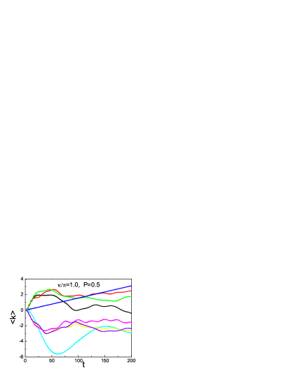
Figure 1: (Color online) The dependence of ratchet current over time for different time delays $\eta$ at quantum resonance $\kappa=1.0\pi$, with $\eta=1/7,2/7,3/8,1/2,5/9,2/3,7/10,4/5$ represented by the black, red, green, blue, cyan, magenta, and violet lines respectively.

As has been shown in Refs. Lun05 ; Ken08 , we find that there are no accelerated ratchet currents for general values of $\eta$ at the quantum resonance $\kappa=1.0\pi$. But there are ratchet currents at short time interval. What is more, the directions of the currents depend on the time delay between the two sequences of symmetry kicked potentials. For little value of $\eta$, it tends to develop current parallel with the $x$ axis in the first few tens of kicks, while for large value of $\eta$, it tends to get reverse current, as in shown in Figure 1, with the effective strength of the potential $P=0.5$. It indicates that, with different time delays, there are different degrees of imbalance between the left and right sides.

The result is unique at the time delay $\eta=1/2$, as is shown in Fig. 1 that accelerated ratchet current emerges. At the macro-level, the accelerated ratchet current signifies considerable asymmetry between different directions. Here, the broken symmetry is the result of desynchronizing of the two time sequences of symmetry potentials, and the degree of asynchronization can be accessed by the quantity $\textsf{min}\{\frac{\eta}{1-\eta},\frac{1-\eta}{\eta}\}$. Then, at least at the quantum resonance $\kappa=1.0\pi$, time asynchronization can lead to the symmetry breaking of dynamical evolution more efficiently than that induced by instantaneously potentials with broken symmetry in the position space. As can be seen in Fig. 2(a), due to the time delay $\eta=0.5$, the ratchet current created out at $\kappa=1.0\pi$ exceeds that at $\kappa=0.5\pi$ even with a weak potential strength $P=0.5$. In addition, as the time delay $\eta$ increase from 0 to 0.5, the ratchet current at $\kappa=0.5\pi$ becomes larger too. But as demonstrated in Fig. 2(b), the atom with $\eta=0.5$, cannot absorb energy as efficiently as it with $\eta=0$. Fig. 2(c) shows the currents with different strength of potentials over 200 periods. The ratchet current stimulated out of quantum resonance $\kappa=1.0\pi$ with time delay $\eta=0.5$ performs much better than that out of $\kappa=0.5$ without a too much strong potential, so it can be used as new operating point to realize directed transport.

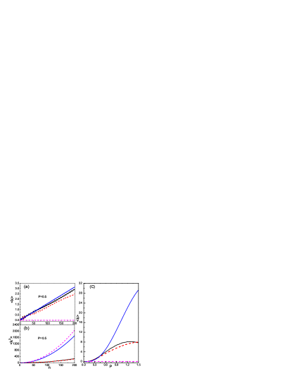
Figure 2: (Color online) The development of (a) the ratchet currents $<k>$ and (b) effective energies $<k^{2}>$, with the strength of potential equals $P=0.5$. (c) Ratchet currents $<k>$ with different values of the potential strength over 200 periods. Here, the dark solid line represents $\kappa=0.5\pi,\eta=0.5$, red dashed line $\kappa=0.5\pi,\eta=0.0$, blue solid line $\kappa=1.0\pi,\eta=0.5$, and magenta dashed line represents $\kappa=1.0\pi,\eta=0.0$.

It is well known that all kinds of properties of the Hamiltonian system are fixed by its energy spectrum. From the microscopic observation, Floquet analysis Lun06 can be exploited to deal with our system due to the fact that the system is subjected to time periodic interactions. The quasienergy spectra of our system at quantum resonance $\kappa=1.0\pi$ and time delay $\eta=0.5$ are given by

$$\omega^{1,3}_{x_{0}} = \pi/4\mp S(x_{0})$$

$$\omega^{1,3}_{x_{0}} = \pi/4\mp\overline{S}(x_{0})$$ (3)

here $S(x)$ and $\overline{S}(x)$ are given by

$$S(x_{0}) = \arctan\bigg{[}\frac{\sqrt{1+\frac{1}{2}\cos^{2}(\overline{v_{2}}(x_{0}))q_{1}(x_{0})}}{\cos(\overline{v_{2}}(x_{0}))p_{1}(x_{0})}\bigg{]}$$

$$\overline{S}(x_{0}) = \arctan\bigg{[}\frac{\sqrt{1+\frac{1}{2}\cos^{2}(\overline{v_{2}}(x_{0}+\frac{\pi}{2}))q_{2}(x_{0})}}{\cos(\overline{v_{2}}(x_{0}+\frac{\pi}{2}))p_{2}(x_{0})}\bigg{]}$$ (4)

with $p_{1}(x_{0})=\cos\big{(}\overline{v_{1}}(x_{0})+\frac{\pi}{4}\big{)}$, $p_{2}(x_{0})=\cos\big{(}\overline{v_{1}}(x_{0})-\frac{\pi}{4}\big{)}$, $q_{1}(x_{0})=\sin\big{(}2\overline{v_{1}}(x_{0})\big{)}-1$, and $q_{2}(x_{0})=\sin\big{(}2\overline{v_{1}}(x_{0})\big{)}+1$. In order to make our expression more compact we have used $\overline{v_{i}}(x)$ in place of $Pv_{i}(x)$, with $i=1,2$.

As is shown in Fig. 3(b), due to the time delay, the quasienergy spectra are split into four bands, with bands $\omega^{1}_{x_{0}}$ ($\omega^{2}_{x_{0}}$) and $\omega^{3}_{x_{0}}$ ($\omega^{4}_{x_{0}}$) intersect at some position of $x_{0}$. While for the case of $\eta=0$ Lun05 ; Ken08 ; Lun06 , as is shown in Fig. 3(a), things are quite different, where there are only two bands of quasienergy spectra without crossing. The corresponding eigenvectors $\alpha^{\rm i}$ at $\eta=0.5$ with ($i=1,2,3,4$) are given by

$$\alpha^{1,3}_{x_{0},0} = \frac{p_{2}(x_{0})e^{-{\rm i}\big{(}\overline{v_{2}}(x_{0})\pm S(x_{0})\big{)}}}{\sqrt{2-2p_{1}(x_{0})\cos\big{(}\overline{v_{2}}(x_{0})\pm S(x_{0})\big{)}}},$$

$$\alpha^{1,3}_{x_{0},2} = \frac{-{\rm i}\big{[}1-p_{1}(x_{0})e^{-{\rm i}\big{(}\overline{v_{2}}(x_{0})\pm S(x_{0})\big{)}}\big{]}}{\sqrt{2-2p_{1}(x_{0})\cos\big{(}\overline{v_{2}}(x_{0})\pm S(x_{0})\big{)}}},$$

$$\alpha^{1,3}_{x_{0},1} = \alpha^{1,3}_{x_{0},3}=0.$$ (5)

and

$$\alpha^{2,4}_{x_{0},1} = \frac{p_{1}(x_{0})e^{-{\rm i}\big{(}\overline{v_{2}}(x_{0}+\frac{\pi}{2})\pm\overline{S}(x_{0})\big{)}}}{\sqrt{2-2p_{2}(x_{0})\cos\big{(}\overline{v_{2}}(x_{0}+\frac{\pi}{2})\pm\overline{S}(x_{0})\big{)}}},$$

$$\alpha^{2,4}_{x_{0},3} = \frac{-{\rm i}\big{[}1-p_{2}(x_{0})e^{-{\rm i}\big{(}\overline{v_{2}}(x_{0}+\frac{\pi}{2})\pm\overline{S}(x_{0})\big{)}}\big{]}}{\sqrt{2-2p_{2}(x_{0})\cos\big{(}\overline{v_{2}}(x_{0}+\frac{\pi}{2})\pm\overline{S}(x_{0})\big{)}}},$$

$$\alpha^{2,4}_{x_{0},0} = \alpha^{2,4}_{x_{0},2}=0,$$ (6)

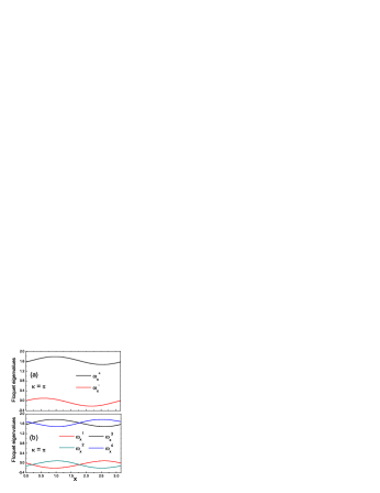
Figure 3: (Color online) Floquet eigenvalues as functions of position $x$, with the strength of potential equals $P=0.5$, at quantum resonance $\kappa=1.0\pi$. (a) The flashing ratchet without time delay $\eta=0$ Lun05 , has two bands of quasienergy spectra. (b) The flashing ratchet with time delay $\eta=1/2$, has four bands of quasienergy spectra.

With the help of these basics elements, the wave function of the system at integer time reads

$$\psi(x,t)=\frac{1}{\sqrt{2\pi}}\sum_{\mu,l,k}\alpha^{\mu*}_{x-l\pi/2,k}e^{-{\rm i}\omega^{\mu}_{x-l\pi/2}t}\alpha^{\mu}_{x-l\pi/2,l}.$$ (7)

The wave function at half integer time can be obtained from the wave function at integer time by reversing the action of the second flashing potential $v_{2}(x)$ and the free evolution of the system with time interval 0.5, so it is given by

$$\psi(x,t-\frac{1}{2}) = \langle x|e^{{rmi}\pi\hat{k}^{2}/4}e^{{\rm i}\overline{v_{2}}(x)}|\psi(x,t)\rangle$$ (8)

$$= \sum_{k=-\infty}^{\infty}e^{{\rm i}\pi k^{2}/4-{\rm i}k(x-x^{\prime})}e^{{\rm i}\overline{v_{2}}(x^{\prime})}\psi(x,t).$$

It can be shown straightforward through a simply numerical simulation that at the limit of large value of $t$, the average force exerted on the atom over one period is a non zero constant. So under the situation of semiclassical, we can now make sure that our numerical results at quantum resonance $\kappa=1.0\pi$ and time delay $\eta=0.5$ demonstrate the real accelerated directed currents. The formulation of the force can be given by

$$\langle\psi(t-\frac{1}{2})|\frac{d\overline{v_{1}}(x)}{dx}|\psi(t-\frac{1}{2})\rangle+\langle\psi(t)|\frac{d\overline{v_{2}}(x)}{dx}|\psi(t)\rangle$$ (9)

$$\propto \int_{0}^{2\pi}dx\bigg{(}\psi^{*}(t-\frac{1}{2})\frac{d\overline{v_{1}}(x)}{dx}\psi(t-\frac{1}{2})$$

$$+ \psi^{*}(t)\frac{d\overline{v_{2}}(x)}{dx}\psi(t)\bigg{)}.$$

In fact, we also find that when we reverse the order of the two symmetry potentials $v_{1}(x)$ and $v_{2}(x)$, there is hardly any difference. For $P=1.0$ the relative difference measured by $|2\times\frac{<k_{1}>-<k_{2}>}{<k_{1}>+<k_{2}>}|$ over 200 periods is 0.7 percent, and for $P=3.0$, it is 0.4 percent (Here $<k_{1}>$ is the average current when $v_{1}(x)$ is first exerted, and $<k_{2}>$ is the average current when $v_{2}(x)$ is first exerted). Current reverse is found around $P=2.6$ for both cases.

It is found that, at time delay $\eta=0.5$, high order quantum resonances can be stimulated to lead to accelerated ratchet currents more efficiently than those at $\eta=0$. An example in point is quantum resonance $\kappa=2.625\pi$, it can induce a ratchet current even at $P=1.5$ much smaller than that without time delay. Another unique low order quantum resonance is $\kappa=3.0\pi$, it can develop directed current as efficiently as $\kappa=1.0\pi$. So it could be valuable for directed transport in biological system, in which the external potential imposed on the organism should be never too strong.

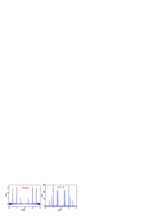
Figure 4: (Color online) Ratchet currents measured by the mean wave number $<k>$ as functions of effective Plank constant $\kappa$ after 200 periods, with $\eta=0.5$. (a) At strength of potential $P=0.5$. (b) At strength of potential $P=1.5$.

In Fig. 4, we show the average wave number $<k>$ over 200 periods, with time delay $\eta=0.5$ for different values of effective Plank constant $\kappa$. As is shown, when the potential strength $P$ increase from 0.5 in Fig. 4(a), to 1.5 in Fig. 4(b), almost all the quantum resonances lead to larger ratchet currents. Higher order quantum resonances begin to surpass the low order ones as the potential strength increase. But quantum resonances $\kappa=1.0\pi$ and $\kappa=3.0\pi$ still mark themselves with large ratchet currents, which are the result of the time asymmetry among the flashing kicks. The other resonances are correlated with both configuration space asymmetry and time series asymmetry whose effects may not be always in phase. We also find that when we reverse the time order of $v_{1}(x)$ and $v_{2}(x)$, there is hardly any difference.

In conclusion, in this paper we have studied the ratchet effect by desynchronizing the two symmetry kicked potentials. It is found that with a time delay $\eta=0.5$ between the two symmetry potentials, quantum resonances $\kappa=1.0\pi$ and $\kappa=3.0\pi$ are stimulated to lead much larger ratchet currents than other quantum resonances at weak potential strength, so they can be chosen as new operating points in order to exploit directed transport. The ratchet effect of $1.0\pi$ ($3.0\pi$) is the result of time asymmetry of the two kicked series of potentials. At this point, time asymmetry may lead to symmetry breaking of the dynamical evolution between different directions more efficiently than that with asymmetry in the position space at discrete times. At the same time, we find that high order quantum resonances can be created out to lead ratchet currents more efficiently than those without a time delay.

This work was supported by National Fundamental Research Program, National Natural Science Foundation of China (Grant Nos.60921091, 10874162).

References

- (1) P. Reimann, Phys. Rep. 361, 57 (2002).
- (2) P. Hänggi and F. Marchesoni, Rev. Mod. Phys. 81, 387 (2009).
- (3) E. M. Roeling, W. C. Germs, B. Smalbrugge, E. J. Geluk, T. de Vries, R. A. Janssen and M. Kemerink, Nat. Mater. 10, 51 (2011).
- (4) R. D. Astumain and P. Hänggi, Phys. Today 55, 33 (2002).
- (5) P. Hänggi and F. Marchesoni and F. Marchesoni and F. Nori, Ann. Phys. 14, 51 (2005).
- (6) P. Jung, J. G. Kissner and P. Hänggi Phys. Rev. Lett. 76, 3436 (1996).
- (7) H. Linke, T. E. Humphrey, A. Löfgren, A. O. Sushkov, R. Newbury, R. P. Taylor and P. Omling, Science 286, 2134 (1999).
- (8) T. S. Monteiro, P. A. Dando, N. A. C. Hutchings and M. R. Isherwood, Phys. Rev. Lett. 89, 194102 (2002).
- (9) J. Gong and P. Brumer, Phys. Rev. Lett. 97, 240602 (2006).
- (10) J. Gong and J. Wang, Phys. Rev. E 76, 036217 (2007).
- (11) L. Chen, C.-F. Li, M. Gong and G.-C. Guo, Phys. A 388, 4328 (2009).
- (12) P. H. Jones, M. M. Stocklin, G. Hur and T. S. Monteiro, Phys. Rev. Lett. 93, 223002 (2004).
- (13) P. H. Jones, M. Goonasekera, D. R. Meacher, T. Jonckheere and T. S. Monteiro, Phys. Rev. Lett. 98, 073002 (2007).
- (14) I. Dana, V. Ramareddy, I. Talukdar and G. S. Summy, Phys. Rev. Lett. 100, 024103 (2008).
- (15) T. Salger, S. Kling, T. Hecking, C. Geckeler, L. M. Molina and M. Weitz, Science 326, 1241 (2009).
- (16) C. Zhang, J. Liu, M. G. Raizen and Q. Niu, Phys. Rev. Lett. 92, 054101 (2004).
- (17) T. S. Monteiro, A. Rançon and J. Ruostekoski, Phys. Rev. Lett. 102, 014102 (2009).
- (18) E. Lundh and M. Wallin, Phys. Rev. Lett. 94, 110603 (2005).
- (19) A. Kenfack, J. Gong and A. K. Pattanayak, Phys. Rev. Lett. 100, 044104 (2008).
- (20) G. Casati, B. V. Chirikov, F. M. Izrailev and J. Ford, Lect. Notes Phys. 93, 334 (1979).
- (21) F. M. Izrailev and D. L. Shepelyanskii, Theor. Math. Phys. 43, 553 (1980).
- (22) D. L. Shepelyanskii, Theor. Math. Phys. 49, 925 (1982).
- (23) S. Fishman, D. R. Grempel and R. E. Prange, Phys. Rev. Lett. 49, 509 (1982).
- (24) B. V. Chirikov and D. L. Shepelyanskii, Radiofizika. 29, 787 (1986).
- (25) F. L. Moore, J. C. Robinson, C. F. Bharucha, B. Sundaram and M. G. Raizen, Phys. Rev. Lett. 75, 4598 (1995).
- (26) M. Lepers, V. Zehnlé and J. C. Garreau, Phys. Rev. A 77, 043628 (2008).
- (27) E. Lundh, Phys. Rev. E 74, 016212 (2006).