Probing neutralino properties in minimal supergravity
with bilinear $R$-parity violation

Abstract

Supersymmetric models with bilinear $R$-parity violation (BRPV) can account for the observed neutrino masses and mixing parameters indicated by neutrino oscillation data. We consider minimal supergravity versions of BRPV where the lightest supersymmetric particle (LSP) is a neutralino. This is unstable, with a large enough decay length to be detected at the CERN Large Hadron Collider (LHC). We analyze the LHC potential to determine the LSP properties, such as mass, lifetime and branching ratios, and discuss their relation to neutrino properties.

I Introduction

Elucidating the electroweak breaking sector of the Standard Model (SM) constitutes a major challenge for the Large Hadron Collider (LHC) at CERN. Supersymmetry provides an elegant way to stabilize the Higgs boson scalar mass against quantum corrections provided supersymmetric states are not too heavy, with some of them expected within reach for the LHC. Searches for supersymmetric particles constitute a major item in the LHC agenda Chatrchyan:2011zy ; daCosta:2011qk ; ATLAS:2011ad ; Aad:2011qa ; Aad:2011cwa ; Aad:2011zj ; Khachatryan:2011tk ; Chatrchyan:2011bz ; Chatrchyan:2011wba ; Chatrchyan:2011ff , as many expect signs of supersymmetry (SUSY) to be just around the corner. However the first searches up to $\sim$ 5 fb^-1 at the LHC interpreted within specific frameworks, such as Constrained Minimal Supersymmetric Standard Model (CMSSM) or minimal supergravity (mSUGRA) indicate that squark and gluino masses are in excess of $\sim 1$ TeV Bechtle:2012zk .

Despite intense efforts over more than thirty years, little is known from first principles about how exactly to realize or break supersymmetry. As a result one should keep an open mind as to which theoretical framework is realized in nature, if any. Supersymmetry search strategies must be correspondingly re-designed if, for example, supersymmetry is realized in the absence of a conserved R parity ATLAS:2011ad ; Aad:2011zb .

Another major drawback of the Standard Model is its failure to account for neutrino oscillations nakamura2010review ; Maltoni:2004ei , whose discovery constitutes one of the major advances in particle physics of the last decade. An important observation is that, if supersymmetry is realized without a conserved R parity, the origin of neutrino masses and mixing may be intrinsically supersymmetric aulakh:1982yn ; hall:1983id ; ross:1984yg ; Ellis:1984gi .

Indeed an attractive dynamical way to generate neutrino mass at the weak scale is through non-zero vacuum expectation values of SU(3) $\otimes$ SU(2) $\otimes$ U(1) singlet scalar neutrinos masiero:1990uj ; romao:1992vu ; romao:1997xf . This leads to the minimal effective description of R parity violation, namely BRPV hirsch:2004he . In contrast to the simplest variants of the seesaw mechanism valle:2006vb such supersymmetric alternative has the merit of being testable in collider experiments, like the LHC decampos:2005ri ; decampos:2007bn ; decampos:2008re ; DeCampos:2010yu . Here we analyze the LHC potential to determine the lightest neutralino properties such as mass, decay length and branching ratios, and discuss their relation to neutrino properties.

II Bilinear $\mathbf{R}$-parity violating SUSY models

The bilinear R-Parity violating models are characterized by two properties: first the usual MSSM R-conserving superpotential is enlarged according to diaz:1997xc

$$W_{\text{BRPV}}=W_{\text{MSSM}}+\varepsilon_{ab}\epsilon_{i}\widehat{L}_{i}^{a}\widehat{H}_{u}^{b}\;,$$ (1)

where there are 3 new superpotential parameters ($\epsilon_{i}$), one for each fermion generation . The second modification is the addition of an extra soft term

$$V_{\text{soft}}=V_{\text{MSSM}}-\varepsilon_{ab}B_{i}\epsilon_{i}\widetilde{L}_{i}^{a}H_{u}^{b}$$ (2)

that depends on three soft mass parameters $B_{i}$. For the sake of simplicity we considered the R-conserving soft terms as in minimal supergravity (mSUGRA). Notice that the presence of the new soft interactions prevents the new bilinear terms in Eq. (1) to be rotated away diaz:1997xc .

The new bilinear terms break explicitly R parity as well as lepton number and induce non-zero vacuum expectation values $v_{i}$ for the sneutrinos. As a result, neutrinos and neutralinos mix at tree level giving rise to one tree–level neutrino mass scale, which we identify with the atmospheric scale. The other two neutrino masses are generated through loop diagrams Hirsch:2000ef ; diaz:2003as . This model provides a good description of the observed neutrino oscillation data Maltoni:2004ei .

The BRPV–mSUGRA model is defined by eleven parameters

$$m_{0}\,,\,m_{1/2}\,,\,\tan\beta\,,\,{\mathrm{sign}}(\mu)\,,\,A_{0}\,,\,\epsilon_{i}\>{\mathrm{,and}}\,\,B_{i}\,,$$ (3)

where $m_{1/2}$ and $m_{0}$ are the common gaugino mass and scalar soft SUSY breaking masses at the unification scale, $A_{0}$ is the common trilinear term, and $\tan\beta$ is the ratio between the Higgs field vacuum expectation values (vevs). In our analyzes the new parameters ($\epsilon_{i}$ and $B_{i}$) are determined by the neutrino masses and mixings, therefore, we have only to vary the usual mSUGRA parameters. For the sake of simplicity in what follows we fix $A_{0}=-100$ GeV, $\tan\beta=10$ and ${\mathrm{sign}}(\mu)>0$ and present our results in the plane $m_{0}\otimes m_{1/2}$.

Due to the smallness of the neutrino masses, the BRPV interactions turn out to be rather feeble, consequently the LSP has a lifetime long enough that its decay appears as a displaced vertex. We show in figure 1 the LSP decay length as a function of $m_{0}$ and $m_{1/2}$, when the remaining values for sign$(\mu),\leavevmode\nobreak\ A$ and $\tan\beta$ are taken as mentioned above. Therefore, we can anticipate that the LSP decay vertex can be observed at the LHC within a large fraction of the parameter space.

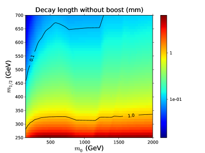
Figure 1: Lightest neutralino decay length as a function of mSUGRA parameters $m_{0}$ and $m_{1/2}$, for $A_{0}=-100$ GeV, $\tan\beta=10$ and ${\mathrm{sign}}(\mu)>0$.

Depending on the SUSY spectrum the lightest neutralino decay channels include fully leptonic decays

$$\tilde{\chi}^{0}_{1}\to\nu\ell^{+}\ell^{-}\;\;\;\;,\;\;\;\;\tilde{\chi}^{0}_{1}\to\nu\tau^{+}\tau^{-}\;\;\;\;\hbox{ and }\;\;\;\;\tilde{\chi}^{0}_{1}\to\nu\tau^{\pm}\ell^{\mp}\,$$

with $\ell=e$ or $\mu$; as well as semi-leptonic decay modes

$$\tilde{\chi}^{0}_{1}\to\nu q\bar{q}\;\;\;\;,\;\;\;\;\tilde{\chi}^{0}_{1}\to\tau q^{\prime}\bar{q}\;\;\;\;,\;\;\;\;\tilde{\chi}^{0}_{1}\to\ell q^{\prime}\bar{q}\;\;\;\;\hbox{ and }\;\;\;\;\tilde{\chi}^{0}_{1}\to\nu b\bar{b}\;.$$

If kinematically allowed, some of these modes take place via two–body decays, like $\tilde{\chi}^{0}_{1}\to W^{\mp}\mu^{\pm}$, $\tilde{\chi}^{0}_{1}\to W^{\mp}\tau^{\pm}$, $\tilde{\chi}^{0}_{1}\to Z\nu$, or $\tilde{\chi}^{0}_{1}\to h\nu$, followed by the $Z$, $W^{\pm}$ or $h$ decay; for further details see Ref. porod:2000hv ; decampos:2007bn . In addition to these channels there is also the possibility of the neutralino decaying invisibly into three neutrinos, however, this channel reaches at most a few per-cent porod:2000hv .

Neutrino masses and mixings as well as LSP decay properties are determined by the same interactions, therefore, there are connections between high energy LSP physics at the LHC and neutrino oscillation physics. For instance, the ratio between charged current decays

$$\frac{\hbox{Br}(\tilde{\chi}^{0}_{1}\to W^{\pm}\mu^{\mp})}{\hbox{Br}(\tilde{\chi}^{0}_{1}\to W^{\pm}\tau^{\mp})}$$ (4)

is directly related to the atmospheric mixing angle datta:1999xq , as illustrated in the right panel of figure 2; this relation was already considered in Ref. DeCampos:2010yu . The vertical bands in figure 2 correspond to the latest 2$\sigma$ precision in the determination of $\theta_{23}$ and $\Delta m_{32}^{2}$ from Ref. Tortola:2012te .

Another interesting interconnection between LSP properties and neutrino properties is the direct relation between neutrino mass squared difference $\Delta m^{2}_{32}$ and the ratio

$$R_{32}=\frac{L_{0}}{\hbox{Br}(\tilde{\chi}^{0}_{1}\to W\ell+Z\nu)}$$ (5)

as is illustrated in left panel of figure 2. Here $L_{0}$ is the LSP decay length and one has to sum over all leptons and neutrinos in the final states. One can understand this relation in the following way. In the BRPV model the tree-level neutrino mass is proportional to $m_{\nu}^{\rm Tree}\propto|\Lambda|^{2}$, where $|\Lambda|^{2}=\sum_{i}\Lambda_{i}^{2}$, with $\Lambda_{i}=\epsilon v_{d}+\mu v_{i}$, is the so-called alignment vector. Couplings between the gauginos and gauge bosons plus leptons/neutrinos are proportional to $\Lambda_{i}$ as well porod:2000hv . Thus, one expects that after summing over the lepton generations the partial width of the neutralino into gauge bosons is also proportional to $|\Lambda|^{2}$. The decay length is the inverse width and dividing by the branching ratio into gauge boson final states picks out the partial width of the neutralino into gauge bosons. This leads to the correlation of $R_{32}$ with the atmospheric neutrino mass scale, since $m_{\rm Atm}$ is identified mostly with $m_{\nu}^{\rm Tree}$, apart from some minor 1-loop corrections.

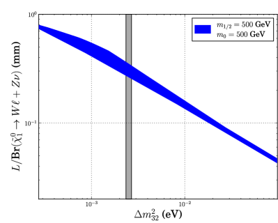
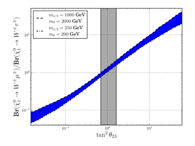
Figure 2: Correlating LSP decay properties with neutrino oscillation parameters. The left panel shows the connection between the displayed LSP decay length parameter and the atmospheric squared mass scale $\Delta m^{2}_{32}$. The right panel depicts the relation between $\hbox{Br}(\tilde{\chi}^{0}_{1}\to W^{\pm}\mu^{\mp})/\hbox{Br}(\tilde{\chi}^{0}_{1}\to W^{\pm}\tau^{\mp})$ and the atmospheric mixing angle. The vertical shaded bands indicate the 2$\sigma$ allowed values of the corresponding neutrino oscillation parameters Tortola:2012te .

III Analyses framework and basic cuts

Our analyzes aim to study the LHC potential to probe the LSP properties exploring its detached vertex signature. We simulated the SUSY particle production using PYTHIA version 6.408 Sjostrand:2000wi ; Sjostrand:1993yb where all the properties of our BRPV-mSUGRA model were included using the SLHA format Skands:2003cj . The relevant masses, mixings, branching ratios, and decay lengths were generated using the SPHENO code Porod:2003um ; Porod:2011nf .

In our studies we used a toy calorimeter roughly inspired by the actual LHC detectors. We assumed that the calorimeter coverage is $|\eta|<5$ and that its segmentation is $\Delta\eta\otimes\Delta\varphi=0.10\times 0.098$. The calorimeter resolution was included by smearing the jet energies with an error

$$\frac{\Delta E}{E}=\frac{0.50}{\sqrt{E}}\oplus 0.03\;.$$

Jets were reconstructed using the cone algorithm in the subroutine PYCELL with $\Delta R=0.4$ and jet seed with a minimum transverse energy $E_{T,min}^{cell}=2$ GeV.

Our analyzes start by selecting events that pass some typical triggers employed by the ATLAS/CMS collaborations, i.e. an event to be accepted should fulfill at least one of the following requirements:

• the event contains one electron or photon with $p_{T}>20$ GeV;

• the event has an isolated muon with $p_{T}>6$ GeV;

• the event exhibits two isolated electrons or photons with $p_{T}>15$ GeV;

• the event has one jet with transverse momentum in excess of 100 GeV;

• the events possesses missing transverse energy greater than 100 GeV.

We then require the existence of, at least, one displaced vertex that is more than $5\sigma$ away from the primary vertex decampos:2007bn – that is, the detached vertex is outside the ellipsoid

$$\left(\frac{x}{5\delta_{xy}}\right)^{2}+\left(\frac{y}{5\delta_{xy}}\right)^{2}+\left(\frac{z}{5\delta_{z}}\right)^{2}=1\;,$$ (6)

where the $z$-axis is along the beam direction. We used the ATLAS expected resolutions in the transverse plane ($\delta_{xy}=20\leavevmode\nobreak\ \mu$m) and in the beam direction ($\delta_{z}=500\leavevmode\nobreak\ \mu$m). To ensure a good reconstruction of the displaced vertex we further required that the LSP decays within the tracking system i.e. within a radius of $550$ mm and $z$–axis length of $3000$ mm. In our model the decay lengths are such that this last requirement is almost automatically satisfied; see figure 1.

IV LSP mass measurement

In order to accurately measure the LSP mass from its decay products we focused our attention on events where the LSP decays into a charged lepton ($e^{\pm}$ or $\mu^{\pm}$) and a $W$ that subsequently decays into a pair of jets. In addition to the basic cuts described above we further required charged leptons to have

$$p_{T}^{\ell}>20\hbox{ GeV and }|\eta_{\ell}|<2.5\;.$$ (7)

We demanded the charged lepton to be isolated, i.e. the sum of the transverse energy of the particles in a cone $\Delta R=0.3$ around the lepton direction should satisfy

$$\sum_{\Delta R<0.3}E_{T}<5\hbox{ GeV}\;.$$ (8)

We identified the hadronically decaying $W$ requiring that its decay jets are central

$$p_{T}^{j}>20\hbox{ GeV}\;\;\;\;,\;\;\;\;|\eta_{j}|<2.5\;,$$ (9)

and that their invariant mass is compatible with the $W$ mass:

$$|\eta_{j}|<2.5\;\;\;\;\hbox{and}\;\;\;\;|M_{jj}-M_{W}|<20\hbox{ GeV}\;.$$ (10)

In order to obtain the LSP mass, we considered points in the $m_{0}\otimes m_{1/2}$ plane with more than 10 expected events for an integrated luminosity of 100 fb^-1. We have performed a Gaussian fit to the lepton–jet–jet invariant mass; as an illustration of the lepton–jet–jet invariant mass spectrum see figure 3. As we can see from this figure, the actual LSP mass (101 GeV) is with 1% of its fitted value (100.4 GeV).

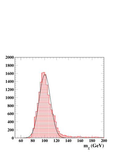
Figure 3: Illustration of the lepton–jet–jet invariant mass spectrum fitted to obtain the LSP mass. In this figure we considered $m_{0}=250$ GeV, $m_{1/2}=250$ GeV, $\tan\beta=10$, $A_{0}=-100$ GeV, and $\hbox{sgn}(\mu)>0$ which leads to a LSP mass of 101 GeV.

In order to better appreciate the precision with which the LSP mass can be determined for other choices of mSUGRA parameters we have repeated the analysis for a wide grid of values in the $m_{0}\otimes m_{1/2}$ plane. The left panel of figure 4 depicts the achievable precision in the LSP mass measurement for an integrated luminosity of 100 fb^-1 as a function of $m_{0}\otimes m_{1/2}$ for $A_{0}=-100$ GeV, $\tan\beta=10$, and $\hbox{sgn}(\mu)>0$. As one can see the LSP mass can be measured with an error between 10 and 15 GeV within a sizeable fraction of the ($m_{0}\otimes m_{1/2}$) plane. Only at high $m_{1/2}$ there is a degradation of the precision due to poor statistics. The right panel in figure 4 shows that indeed this is enough to determine the LSP mass to within 5 to 10% in a relatively wide chunk of parameter space.

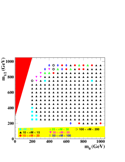
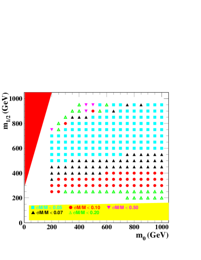
Figure 4: The left panel presents the error ($\sigma_{M}$) on the LSP mass as a function of the $m_{0}\otimes m_{1/2}$ point for $A_{0}=-100$ GeV, $\tan\beta=10$, $\hbox{sgn}\mu>0$ and an integrated luminosity of 100 fb^-1, while the right panel displays the relative error in the LSP mass determination $\sigma_{M}/M_{\tilde{\chi}^{0}_{1}}$.

V LSP decay length measurement

Another important feature of the LSP in our BRPV-mSUGRA model is its decay length (lifetime). Within the simplest mSUGRA bilinear R parity violating scheme this is directly related to the squared mass splitting $\Delta m_{32}^{2}$, well measured in neutrino oscillation experiments Tortola:2012te . In this analysis we considered events where the LSP decay contains at least three charged tracks, i.e. the LSP decays into $\ell jj$, with $\ell=e$ or $\mu$. Here we sum over all jets as well as over $\tilde{\chi}^{0}_{1}\to\ell W\to\ell jj$ and all three body decays leading to the same final state.

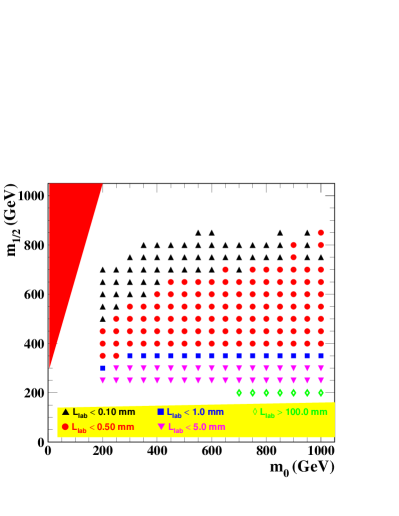
Figure 5: Average distance traveled by the LSP in the laboratory frame as a function of the $m_{0}\otimes m_{1/2}$ point for $A_{0}=-100$ GeV, $\tan\beta=10$, and sgn $\mu>0$.

In figure 5 we depict the average distance traveled by the LSP as observed in the laboratory frame. As we can see, a substantial fraction of the LSP decays takes place within the pixel detector, except for very low $m_{1/2}$ values. It is interesting to notice that the pattern shown in the figure is similar to the one in figure 1, as we could easily expect. Since most of the LSP decays occur inside the beam pipe we can anticipate a small backgrounds associated to particles scattering in the detector material.

In order to obtain the LSP decay length ($L_{0}$) from the distance traveled in the laboratory frame ($d$) we considered the $m_{obs}d/p_{obs}$ distribution, with $m_{obs}$ ($p_{obs}$) being the measured invariant mass (momentum) associated to the displaced vertex, and then we fitted it with an exponential

$$e^{-\frac{m_{obs}d}{p_{obs}L_{0}}}$$

where the fitting parameter ($L_{0}$) is the LSP decay length.

In order to disentangle the energy and momentum uncertainties and the statistical errors from the intrinsic limitation associated to the tracking we first neglect the latter one. In the left panel of figure 6 we present the expected precision in the decay length determination in the plane $m_{0}\otimes m_{1/2}$ for an assumed integrated luminosity of 100 fb^-1. As one can see, these sources of error have a small impact in the determination of the decay length, except for heavier LSP masses where we run out of statistics. In fact, the contribution of these sources of uncertainty is smaller than 5% for neutralino masses up to 280 GeV ($m_{1/2}\simeq 700$ GeV).

Clearly, the actual achievable precision of LSP lifetime determination at the LHC experiments depends on the ability to measure the LSP traveled distance in the laboratory. We present in the right panel of figure 6 the attainable precision on the decay length assuming a 10% tracking error ross:2011pr in the LSP flight distance to get a rough idea. Clearly the precision in the decay length gets deteriorated, however, it is still better than 15% within a relatively large fraction of the parameter space under this assumption but would get corresponding worse if this uncertainty were larger.

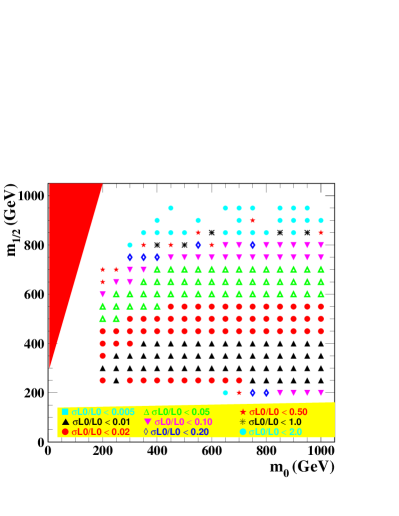
Figure 6: Relative error ($\sigma_{L_{0}}/L_{0}$) in the determination of the LSP decay length as a function of the $m_{0}\otimes m_{1/2}$ for $A_{0}=-100$ GeV, $\tan\beta=10$, sgn $\mu>0$, and an integrated luminosity of 100 fb^-1. The left (right) panel assumes no error (10% error) in the measurement of distance traveled by the LSP.

VI LSP Branching ratio measurements

As we have already mentioned, the neutrino mass squared difference $\Delta m_{32}^{2}$ controls the ratio given in Eq. 5, therefore we should also study how well the neutralino LSP decay ratio into $\ell W$ and $\nu Z$ can be determined. In order to illustrate the LHC capabilities in probing LSP properties at high energies we present the reconstruction efficiency for the benchmark scenario

$$m_{1/2}=250\hbox{ GeV }\;\;\hbox{and}\;\;m_{0}=250\hbox{ GeV}$$

that yields a rather light LSP ($m_{\rm LSP}\simeq 101$ GeV) and heavy scalars. For this point in parameter space the LSP possesses a decay length $c\tau=30$ $\mu$m and its dominant decay modes have the following branching ratios:

$$\begin{array}[]{lcrlcrlcr}\mathrm{BR}(\tilde{\chi}_{1}^{0}\to W^{\pm}e^{\mp})&=&0.2\%,&\mathrm{BR}(\tilde{\chi}_{1}^{0}\to W^{\pm}\mu^{\mp})&=&27.6\%,&\mathrm{BR}(\tilde{\chi}_{1}^{0}\to W^{\pm}\tau^{\mp})&=&31.3\%,\\ \mathrm{BR}(\tilde{\chi}_{1}^{0}\to b\bar{b}\nu)&=&7.1\%,&\mathrm{BR}(\tilde{\chi}_{1}^{0}\to Z\nu)&=&11.9\%,&\\ \mathrm{BR}(\tilde{\chi}_{1}^{0}\to e^{\pm}\tau^{\mp}\nu)&=&5.5\%,&\mathrm{BR}(\tilde{\chi}_{1}^{0}\to\mu^{\pm}\tau^{\mp}\nu)&=&5.5\%,&\mathrm{BR}(\tilde{\chi}_{1}^{0}\to\tau^{\pm}\tau^{\mp}\nu)&=&9.5\%\end{array}$$

$N_{eqq^{\prime}}$	$N_{\mu qq^{\prime}}$	$N_{\tau qq^{\prime}}$	$N_{e\tau\nu}$	$N_{\mu\tau\nu}$	$N_{\tau\tau\nu}$
0.291	0.106	0.011	0.087	0.126	0.061

Table 1: Reconstruction efficiencies for neutralino LSP decays for our benchmark point. For the $\tau$ lepton only hadronic final states have been considered while the $\tau$ decays into electrons and muons were included in the first two entries.

We present in Table 1 the reconstruction efficiencies of the LSP decay modes for our chosen benchmark point. The reconstruction efficiencies for final states containing $\tau$’s are much smaller, as expected, leading to a loss of statistics in these final states. For an exhaustive study of the reconstruction efficiencies see Ref. DeCampos:2010yu .

We present in figure 7 the expected error on the LSP branching ratio $\hbox{Br}(\tilde{\chi}^{0}_{1}\to\ell W+\nu Z)$ as a function $m_{0}\otimes m_{1/2}$ for an integrated luminosity of 100 fb^-1. In order to evaluate this error we studied the reconstruction efficiency for this final state and simulated 100 fb^-1 of data for several points in the $m_{0}\otimes m_{1/2}$ plane. As one can see, this branching ratio can be well determined in the regions of large production cross section, i.e. small $m_{0}$ and $m_{1/2}$. Although for heavier neutralinos the precision diminishes, still this branching ratio can be determined to within 20% in a large portion of the parameter space. In order to study the possibility of LHC to probe the atmospheric mass, we have evaluated Br$(\tilde{\chi}^{0}_{1}\rightarrow W\ell)$ + Br$(\tilde{\chi}^{0}_{1}\to Z\nu)$ appearing in Eq. 5. The $W\ell$ channel is obtained by first reconstructing displaced vertices with hadronic $W$ decays, $jj\ell$, in the final state. Beside the cuts described in sections III and IV we have applied an invariant mass cut on the jet pair: $|M_{W}-M_{jj}|<20$ GeV to disentangle the $W$-contribution to this final state. Afterward we get the branching ratio for $W\ell$ using

$$\mathrm{Br}(\tilde{\chi}^{0}_{1}\rightarrow W\ell)=\frac{\mathrm{Br}(\tilde{\chi}^{0}_{1}\rightarrow jj\ell)}{N_{lqq^{\prime}}}\times\left(1+\frac{\mathrm{Br}(W\rightarrow\ell\nu)}{\mathrm{Br}(W\rightarrow qq\prime)}\right)\;\;.$$ (11)

The $Z\nu$ channel was calculated similarly by reconstructing the displaced vertices with hadronic $Z$ decays, $jj\nu$, in the final state and properly rescaling it. Also here we have applied an invariant mass cut on the jet pair: $|M_{Z}-M_{jj}|<20$ GeV.

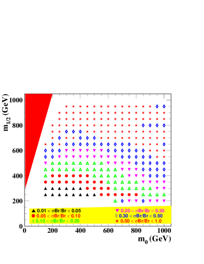
Figure 7: Expected error on the $\hbox{Br}(\tilde{\chi}^{0}_{1}\to\ell W+\nu Z)$ as a function $m_{0}\otimes m_{1/2}$ for an integrated luminosity of 100 fb^-1.

VII LSP properties and atmospheric neutrino oscillations

As seen in Section II, the MSSM augmented with bilinear $R$–parity violation exhibits correlations between LSP decay properties and the neutrino oscillation parameters Hirsch:2000ef ; diaz:2003as , which are by now well measured in neutrino oscillation experiments Tortola:2012te . In particular the squared mass difference $\Delta m_{32}^{2}$ is connected to the ratio $R_{32}$ between the LSP decay length and its branching ratio into $\ell W$ and $\nu Z$; see the right panel of figure 2. In figure 8 we display the expected accuracy on the ratio $R_{32}$ as a function of $m_{0}\otimes m_{1/2}$ for an integrated luminosity of 100 fb^-1 and assuming 10% precision in the determination of the LSP traveled distance. As we can see $R_{32}$ can be determined with a precision 20–30% in a large fraction of the $m_{0}\otimes m_{1/2}$ plane and, as expected, the precision is lost for heavy LSPs. For small LSP masses the error on $R_{32}$ is dominated by the uncertainty on the decay length, while for heavier LSPs the dominant contribution comes from the branching ratio determination due to the limited statistics.

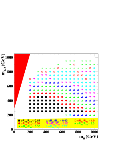
Figure 8: Expected accuracy on the ratio $R_{32}$ as a function of $m_{0}\otimes m_{1/2}$ for an integrated luminosity of 100 fb^-1.

It is interesting to notice from the right panel of figure 2 that a measurement of $R_{32}$ with 20–30% precision it is enough to determine the correct magnitude of $\Delta m_{32}^{2}$ using the BRPV-mSUGRA framework. Nevertheless, a much higher precision is needed to obtain uncertainties similar to the neutrino experiments such as MINOS/T2K Tortola:2012te . On the other hand, the relation between the atmospheric mixing angle and the ratio of the LSP branching ratios into $\tau W$ and $\mu W$ can lead to more stringent tests of the BRPV–mSUGRA model. In Ref. DeCampos:2010yu it was shown that this ratio can be determined at the LHC with a precision better than 20% in a large fraction of the $m_{0}\otimes m_{1/2}$ plane. From figure 2 we can see that this precision is enough to have a determination for $\tan^{2}\theta_{23}$ with an error similar to the low energy neutrino oscillation measurements. Looking from a different point of view, the collider data can be combined with neutrino data to determine the underlying parameters of the model. In this case collider and neutrino data give ’orthogonal’ information as has been shown in Thomas:2011kt .

VIII Conclusions

We have analyzed the LHC potential to determine the LSP properties, such as mass, lifetime and branching ratios, within minimal supergravity with bilinear $R$-parity violation. We saw that the LSP mass determination is rather precise, while the LSP lifetime and branching ratios can be determined with a 20% error in a large fraction of the parameter space. This is enough to allow for qualitative test of the BRPV–mSUGRA model using the $R_{32}$–$\Delta m_{32}^{2}$ correlation. On the other hand, semi-leptonic LSP decays to muons and taus correlate extremely well with neutrino oscillation measurements of $\theta_{23}$.

In the BRPV model for low values of $M_{1/2}$ one can have sizeable branching ratios into the final states $e\tau\nu$ and $\mu\tau\nu$. These decays are potentially interesting for testing another aspects of the model associated with solar neutrino physics. As shown in diaz:2003as in regions of parameter space where the scalar taus are not very heavy, usually the loop with taus-staus in the diagram dominates the 1-loop neutrino mass. In this case the solar angle is predicted to be proportional to $(\tilde{\epsilon}_{1}/\tilde{\epsilon}_{2})^{2}\propto\tan^{2}\theta_{\odot}$. Here, $\tilde{\epsilon}=V_{\nu}^{T,tree}{\vec{\epsilon}}$, with $V_{\nu}^{T,tree}$ being the matrix which diagonalizes the tree-level neutrino mass. Note that $V_{\nu}^{T,tree}$ is entirely determined in terms of the $\Lambda_{i}$. In the BRPV model, RPV couplings of the scalar tau are proportional to the superpotential parameters $\epsilon_{i}$. Ratios of the decays Br$(\chi^{0}_{1}\to e\tau\nu)/$Br$(\chi^{0}_{1}\to\mu\tau\nu)$ are then given, to a very good approximation by Br$(\chi^{0}_{1}\to e\tau\nu)/$Br$(\chi^{0}_{1}\to\mu\tau\nu)\propto(\epsilon_{1}/\epsilon_{2})^{2}$. If the $\Lambda_{i}$ where known, this could be turned into a test of the prediction for the solar angle. Note that in the limit where the reactor angle is exactly zero and the atmospheric angle exactly maximal one obtains $(\tilde{\epsilon}_{1}/\tilde{\epsilon}_{2})^{2}=2(\epsilon_{1}/\epsilon_{2})^{2}$. However, the $\Lambda_{i}$ are currently not well fixed, due to the comparatively large uncertainty in the atmospheric angle. Thus the correlation between three-body leptonic decays of the neutralino with tau final states and the solar angle has a rather large uncertainty. This prevents a stringent consistency test of the model using these decays.

All in all we have shown that neutralino decays can be used to extract some of their properties rather well in models with bilinear $R$-parity violation. Properties such as the decay length and the ratio of semi-leptonic decay branching ratios to muons and taus correlate rather well with atmospheric neutrino oscillation parameters. These features should also apply to schemes where the gravitino is the LSP and the neutralino is the next to lightest SUSY particle Hirsch:2005ag ; Restrepo:2011rj . For gravitino masses in the allowed range where it plays the role of cold dark matter, its R-parity conserving decays are negligible compared to its R parity violating decays. The latter follow the same patter studied in the present paper, so that the results derived here should also hold.

References

- (1) CMS Collaboration, S. Chatrchyan et al., Phys.Rev.Lett. 107, 221804 (2011), arXiv:1109.2352.
- (2) Atlas Collaboration, G. Aad et al., Phys.Lett. B701, 186 (2011), arXiv:1102.5290.
- (3) ATLAS Collaboration, G. Aad et al., Phys.Rev. D85, 012006 (2012), arXiv:1109.6606.
- (4) Atlas Collaboration, G. Aad et al., JHEP 1111, 099 (2011), arXiv:1110.2299.
- (5) ATLAS Collaboration, G. Aad et al., Phys.Lett. B709, 137 (2012), arXiv:1110.6189.
- (6) ATLAS Collaboration, G. Aad et al., Phys.Lett. B710, 519 (2012), arXiv:1111.4116.
- (7) CMS Collaboration, V. Khachatryan et al., Phys.Lett. B698, 196 (2011), arXiv:1101.1628.
- (8) CMS Collaboration, S. Chatrchyan et al., JHEP 1106, 026 (2011), arXiv:1103.1348.
- (9) CMS Collaboration, S. Chatrchyan et al., JHEP 1106, 077 (2011), arXiv:1104.3168.
- (10) CMS Collaboration, S. Chatrchyan et al., Phys.Lett. B704, 411 (2011), arXiv:1106.0933.
- (11) P. Bechtle et al., (2012), arXiv:1204.4199.
- (12) ATLAS Collaboration, G. Aad et al., Phys.Lett. B707, 478 (2012), arXiv:1109.2242.
- (13) K. Nakamura et al., Journal of Physics G: Nuclear and Particle Physics 37, 075021 (2010).
- (14) M. Maltoni, T. Schwetz, M. A. Tortola, and J. W. F. Valle, New J. Phys. 6, 122 (2004), hep-ph/0405172.
- (15) C. S. Aulakh and R. N. Mohapatra, Phys. Lett. B119, 13 (1982).
- (16) L. J. Hall and M. Suzuki, Nucl. Phys. B231, 419 (1984).
- (17) G. G. Ross and J. W. F. Valle, Phys. Lett. B151, 375 (1985).
- (18) J. R. Ellis and et al., Phys. Lett. B150, 142 (1985).
- (19) A. Masiero and J. W. F. Valle, Phys. Lett. B251, 273 (1990).
- (20) J. C. Romao, C. A. Santos, and J. W. F. Valle, Phys. Lett. B288, 311 (1992).
- (21) J. C. Romao, A. Ioannisian, and J. W. F. Valle, Phys. Rev. D55, 427 (1997), hep-ph/9607401.
- (22) M. Hirsch and J. W. F. Valle, New J. Phys. 6, 76 (2004).
- (23) J. W. F. Valle, J. Phys. Conf. Ser. 53, 473 (2006), hep-ph/0608101, Review lectures at Corfu.
- (24) F. de Campos et al., Phys. Rev. D71, 075001 (2005), hep-ph/0501153.
- (25) F. de Campos et al., JHEP 05, 048 (2008).
- (26) F. de Campos, O. J. P. Eboli, M. B. Magro, and D. Restrepo, Phys. Rev. D79, 055008 (2009), arXiv:0809.0007.
- (27) F. De Campos et al., Phys. Rev. D82, 075002 (2010).
- (28) M. A. Diaz, J. C. Romao, and J. W. F. Valle, Nucl. Phys. B524, 23 (1998).
- (29) H.-P. Nilles and N. Polonsky, Nucl. Phys. B484, 33 (1997), hep-ph/9606388.
- (30) G. F. Giudice and A. Masiero, Phys. Lett. B206, 480 (1988).
- (31) M. Hirsch et al., Phys. Rev. D62, 113008 (2000), hep-ph/0004115, Err-ibid. D65:119901,2002.
- (32) M. A. Diaz et al., Phys. Rev. D68, 013009 (2003).
- (33) W. Porod et al., Phys. Rev. D63, 115004 (2001).
- (34) M. Gonzalez-Garcia, J. Romao, and J. Valle, Nucl.Phys. B391, 100 (1993).
- (35) A. Bartl et al., Nucl.Phys. B502, 19 (1997), arXiv:hep-ph/9612436.
- (36) M. Hirsch and W. Porod, Phys. Rev. D74, 055003 (2006), arXiv:hep-ph/0606061.
- (37) M. Hirsch, A. Vicente, and W. Porod, Phys. Rev. D77, 075005 (2008), arXiv:0802.2896.
- (38) A. Datta, B. Mukhopadhyaya, and F. Vissani, Phys. Lett. B492, 324 (2000), hep-ph/9910296.
- (39) D. Forero, M. Tortola, and J. Valle, (2012), arXiv:1205.4018, this updates previous results in New J.Phys. 13 (2011) 109401 and New J.Phys. 13 (2011) 063004 by including recent Double Chooz, Daya-Bay and RENO reactor measurements.
- (40) T. Sjostrand et al., Comput. Phys. Commun. 135, 238 (2001), hep-ph/0010017.
- (41) T. Sjostrand, Comput. Phys. Commun. 82, 74 (1994).
- (42) P. Skands et al., JHEP 07, 036 (2004), hep-ph/0311123.
- (43) W. Porod, Comput. Phys. Commun. 153, 275 (2003), hep-ph/0301101.
- (44) W. Porod and F. Staub, (2011), arXiv:1104.1573.
- (45) E. Ross, private communication.
- (46) F. Thomas and W. Porod, JHEP 1110, 089 (2011), arXiv:1106.4658.
- (47) M. Hirsch, W. Porod and D. Restrepo, JHEP 0503, 062 (2005) [hep-ph/0503059].
- (48) D. Restrepo, M. Taoso, J. Valle, and O. Zapata, Phys.Rev. D85, 023523 (2012), arXiv:1109.0512.