A Coronal Hole’s Effects on CME Shock Morphology in the Inner Heliosphere

Abstract

We use STEREO imagery to study the morphology of a shock driven by a fast coronal mass ejection (CME) launched from the Sun on 2011 March 7. The source region of the CME is located just to the east of a coronal hole. The CME ejecta is deflected away from the hole, in contrast with the shock, which readily expands into the fast outflow from the coronal hole. The result is a CME with ejecta not well centered within the shock surrounding it. The shock shape inferred from the imaging is compared with in situ data at 1 AU, where the shock is observed near Earth by the Wind spacecraft, and at STEREO-A. Shock normals computed from the in situ data are consistent with the shock morphology inferred from imaging.

1 INTRODUCTION

One aspect of space weather forecasting involves the prediction of coronal mass ejection (CME) arrival times at Earth, which may or may not lead to a geomagnetic storm at that time. Assuming it is reasonably well established that a solar eruption is indeed headed towards Earth, an accurate assessment of its arrival time depends on both an accurate measurement of the CME’s initial velocity, and some estimate of how that velocity will change during its passage through the interplanetary medium (IPM).

The STEREO mission (Kaiser et al., 2008; Howard et al., 2008) provides substantial improvements in our ability to study both these aspects of CME kinematics. The lateral views that the two STEREO spacecraft have of the Sun-Earth line provide ideal vantage points for measuring the radial velocities of Earth-directed CMEs. In contrast, from the perspective of a near-Earth instrument such as the Large Angle Spectrometric Coronagraph (LASCO) instrument (Brueckner et al., 1995) on board the Solar and Heliospheric Observatory (SOHO), an observer will only be able to perceive the lateral expansion of the CME. As for IPM propagation, the heliospheric imagers on board the two STEREO spacecraft allow for continuous CME tracking all the way to 1 AU.

We will be studying here the effects of the ambient solar wind on a shock generated by a fast CME originating on 2011 March 7. The source region of the CME is just to the east of a coronal hole, which has a dramatic effect on the shape of the shock both close to the Sun and in the IPM. The western half of the shock propagates outwards through high speed wind from the coronal hole, ultimately hitting STEREO-A on March 9, while the eastern half propagates outwards through slow speed wind, ultimately hitting Earth a day later on March 10. In addition to the indications of shock deformation provided by the in situ data, heliospheric images of the event also show signatures of the uneven shock geometry caused by the high speed wind from the coronal hole. This is therefore an ideal event for studying the effects of an inhomogeneous solar wind on shock morphology. We will empirically reconstruct the shock shape from the data, and we will also examine whether MHD models of the inner heliosphere can successfully reproduce the inferred shape.

2 OBSERVATIONS

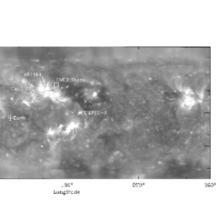
Figure 1: Carrington map of the solar corona for Carrington rotation 2107, based on EUVI $\lambda$195 images from STEREO-A. The two 2011 March 7 CMEs originate in the labeled active regions AR1166 and AR1164. The central trajectories of the flux rope (FR) components of the two CMEs are indicated, as is the inferred central trajectory of the CME2 shock.

Figure 1 shows a Carrington map of EUV emission from the solar corona, for Carrington rotation number 2107, created from 195 Å bandpass EUVI images from STEREO-A. The positions of Earth, STEREO-A, and STEREO-B are indicated for 2011 March 7. At this time, STEREO-A was located $87.6^{\circ}$ ahead of Earth in its orbit around the Sun, at a distance of 0.96 AU from Sun-center, and STEREO-B was $94.9^{\circ}$ behind Earth, at a distance of 1.02 AU. Figure 2 explicitly displays the spacecraft geometry in the ecliptic plane, in heliocentric aries ecliptic coordinates.

There are two CMEs on 2011 March 7 that we will be modeling, one from active region AR1166, and one from AR1164. The locations of these two active regions are identified in Figure 1. The first CME, which we will call CME1, begins with an M1.9 flare from AR1166 at 13:45, while the second CME, CME2, begins with an M3.7 flare from AR1164 at 19:43. It is the second event that we are primarily interested in, but the two CMEs end up overlapping in the inner heliosphere, so it is necessary to consider observations of both.

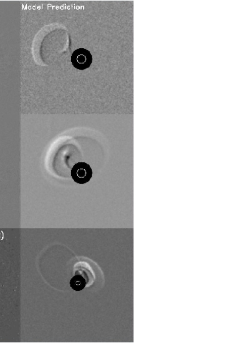
Figure 3: Coronagraphic images of the two 2011 March 7 CMEs from COR2 on STEREO-A and C3 on SOHO/LASCO. Actual images are on the left, and on the right are synthetic images of the CMEs derived from the 3-D reconstruction of the events described in section 4.

Each STEREO spacecraft carries a package of imagers called the Sun-Earth Connection Coronal and Heliospheric Investigation (SECCHI), which includes two coronagraphs (COR1 and COR2) and two heliospheric imagers (HI1 and HI2) that observe CMEs both close to the Sun and in the inner heliosphere (Howard et al., 2008; Eyles et al., 2009). The fields of view of HI1 and HI2 are illustrated in Figure 2. The top two panels of Figure 3 show images of the two March 7 CMEs as seen from STEREO-A’s perspective, specifically by the COR2-A telescope. These images, and all other images shown in this paper, are displayed in running difference format, where the previous image is subtracted from each image to effectively remove static coronal structures and emphasize the dynamic CME.

The second CME consists of two distinct components: the ejecta, which is directed towards the northeast in the image, and a bright front out ahead of the ejecta, which is the shock wave created by this fast, supersonic CME. Curiously, the ejecta is not at all well centered within the shock, in contrast to other CMEs with visible shocks that we have studied recently (Wood & Howard, 2009; Wood et al., 2011). Although both the ejecta and shock have a northward component to their trajectory, the shock appears centered more to the west than the ejecta (i.e., more towards STEREO-A). We attribute this asymmetry to the presence of a coronal hole just to the west of the CME’s source region, as shown in Figure 1. Studying the effects of the coronal hole on this shock’s morphology is the focal point of this paper.

In contrast to CME2, there is no bright front out ahead of CME1 indicative of a shock, presumably because CME1 is a much slower eruption and is not able to create a bright shock front. In COR2-A, the ejecta of the two CMEs are both directed towards the northeast, both possessing an angular extent of about $90^{\circ}$. The more easterly longitude of CME1 is indicated both by the location of its source region relative to that of CME2 (see Figure 1) and by LASCO images of the two CMEs. The bottom panel of Figure 3 is a LASCO/C3 image in which both events are seen, with CME1 directed somewhat to the northeast of the Sun-Earth line, and the brighter CME2 directed to the northwest.

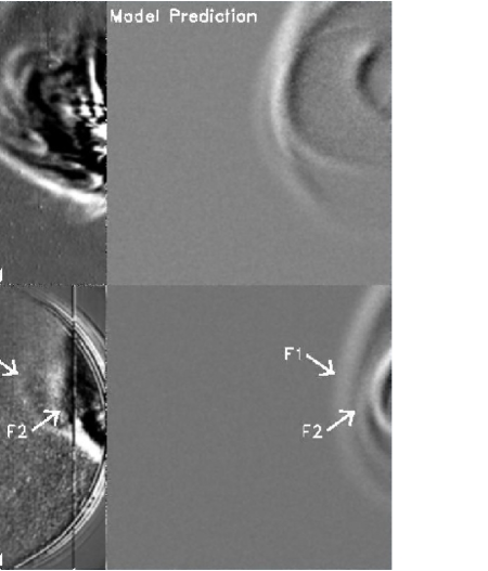
Figure 4: Heliospheric images of CME2 from STEREO-A. Actual images are on the left, and on the right are synthetic images of the CMEs derived from the 3-D reconstruction of the CME (see section 4). The fronts labeled F1 and F2 are both associated with the CME2 shock. Figure 2 illustrates our interpretation of these two fronts as being the consequence of an asymmetric shock shape.

Both 2011 March 7 CMEs can be tracked all the way to 1 AU using STEREO’s heliospheric imagers. For CME1, STEREO-B provides a better vantage point for tracking the CME into the inner heliosphere, while for CME2 STEREO-A is better. Figure 4 shows HI1-A and HI2-A images of CME2. In HI1-A, CME2 quickly overtakes CME1, such that by the time of the image in Figure 4 the two CMEs are superimposed on each other, complicating interpretation of the data. Although the expansion rate of CME2 slows dramatically in HI1-A, its leading edge still moves well in front of CME1, and in the HI2-A image in Figure 4, the CME front seen is entirely that of CME2.

As CME2 approaches the left edge of the HI1-A field, the shock at the front of the CME appears to split in two, as a foreground part of the shock appears to move ahead of a background portion. This “doubling” of the shock front becomes even more apparent early in the HI2-A field of view. The two fronts labeled F1 and F2 in the HI2-A image in Figure 4 are both part of the CME2 shock. Our interpretation of this visage is illustrated in Figure 2. The part of the CME2 shock propagating towards STEREO-A in high speed wind emanating from the coronal hole seen in Figure 1 becomes more radially extended than the part of the shock above the ejecta, which is propagating more towards Earth through slow speed wind. This creates a discontinuity in the shock shape in between the longitudes of Earth and STEREO-A, thereby creating two tangent points with the shock as viewed from STEREO-A. The outermost tangent point creates the outermost front, F1, which is the foreground part of the shock from STEREO-A’s vantage point, and the inner tangent point yields the F2 front, corresponding to the slower part of the shock directed more towards Earth. This kind of asymmetry is to be expected on the basis of models of CME propagation into inhomogeneous solar wind (Riley et al., 1997).

To summarize, images from STEREO demonstrate that the coronal hole’s presence near the CME2 source region significantly affects the shape of the CME2 shock. The two main observational signatures of this are the shock not being centered on the ejecta in COR2-A, and the doubling of the shock front in HI2-A. The shock asymmetry can be studied further using in situ data from STEREO-A, and from Wind at the L1 Lagrangian point near Earth. The CME2 shock is broad enough to have hit both spacecraft, despite a nearly $90^{\circ}$ separation in longitude.

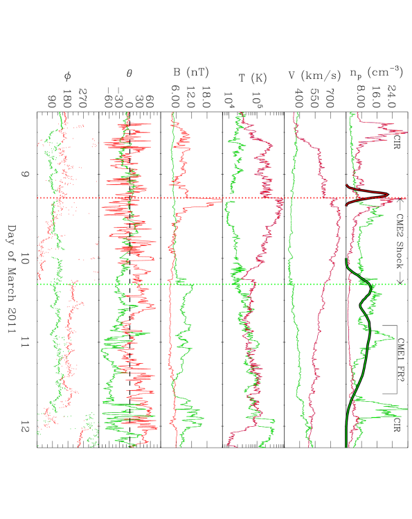
Figure 5: In situ observations of solar wind plasma parameters from STEREO-A (red) and Wind (green). The parameters are, from top to bottom, proton density, velocity, temperature, magnetic field, poloidal magnetic field direction, and azimuthal magnetic field direction. Vertical dotted lines indicate the location of the CME2 shock, at both STEREO-A and Wind. The thick lines in the density panel show the density profiles expected at STEREO-A and Wind based on the 3-D empirical reconstruction described in section 4.

Figure 5 shows plasma parameters measured at STEREO-A and Wind. Focusing first on STEREO-A, where the meaurements are made by the PLASTIC and IMPACT instruments on board the spacecraft (Acuña et al., 2008; Galvin et al., 2008; Luhmann et al., 2008), on March 8 there is a density peak accompanied by a dramatic increase in wind speed and temperature, indicating that this is a corotating interaction region (CIR) associated with the high speed wind emanating from the coronal hole just to the west of the CME2 source region (AR1164; see Figure 1). The shock of CME2 hits STEREO-A at about 6:48 UT on March 9, indicated by substantial jumps in density, velocity, temperature, and magnetic field. After a CME shock, a signature of the CME ejecta driving the shock is often observed. That is not the case at STEREO-A, where nothing but normal high speed wind follows the shock. This is an excellent example of the “driverless shocks” studied by Gopalswamy et al. (2009). The lack of a driver at STEREO-A is not a surprise based on the apparent trajectory of the ejecta away from the Sun-spacecraft line in COR2-A (see Figure 3).

The CME2 shock also hits Wind, but it does so over a day later at about 7:44 UT on March 10 (see Figure 5). This delayed arrival time is consistent with the shock shape displayed in Figure 2. The shock arrival time discrepancy between STEREO-A and Wind provides another valuable diagnostic for the degree of asymmetry in the shock induced by the coronal hole and its high speed wind.

Unlike at STEREO-A, there is ejecta observed following the CME2 shock at Earth. Not only is there a large density peak associated with this ejecta, but a lengthy period of negative $B_{z}$ on March 10–11 (see $\theta$ panel in Figure 5), which produces a modest but lengthy geomagnetic storm at this time, with the planetary K index reaching as high as $K_{p}=6$. The question is whether the ejecta is from CME1 or CME2. For that matter, how sure are we that the shock seen by Wind is associated with CME2 instead of CME1? We will return to these issues after describing in detail how we have tried to empirically reconstruct the morphology and kinematics of the two 2011 March 7 CMEs.

3 KINEMATIC MODELS

Kinematic modeling of CME1 and CME2 is a necessary aspect of their 3-D reconstruction. For both CMEs we track the leading edge of the ejecta (as opposed to the shock in the case of CME2). For CME1, STEREO-B provides the best vantage point to view the CME’s IPM propagation, so STEREO-B images are used to measure its elongation angle, $\epsilon$, from Sun-center as a function of time. For CME2, STEREO-A images are used instead. These elongation angles are converted to actual distances from Sun-center, $r$, using the equation first championed by Lugaz et al. (2009),

$$r=\frac{2d\sin\epsilon}{1+\sin(\epsilon+\phi)},$$ (1)

where $d$ is the observer’s distance to the Sun, and $\phi$ is the angle between the CME trajectory and the observer’s line of sight to the Sun. This equation is derived assuming that CME fronts can be approximated as spheres centered halfway in between their leading edges and the Sun. By at least crudely taking into account a CME’s lateral extent, this equation will be applicable to more viewing geometries than the alternative “Fixed-$\phi$” approxmiation (Kahler & Webb, 2007; Sheeley et al., 2008; Wood et al., 2010),

$$r=\frac{d\sin\epsilon}{\sin(\epsilon+\phi)},$$ (2)

which assumes an infinitely narrow CME. However, for the advantageous near-lateral viewing geometries that we have here for CME1 and CME2, both equations will yield similar results (Lugaz et al., 2011).

Measurements of the CME trajectory angle $\phi$ are ultimately established by the morphological modeling described in section 4. For CME1, $\phi=70^{\circ}$ (from STEREO-B), and for CME2, $\phi=66^{\circ}$ (from STEREO-A). Based on these values and equation (1), Figure 6 shows plots of CME distance versus time for CME1 and CME2. In order to extract velocity profiles from these measurements, we use a simple three-phase kinematic model that we have used before to fit the kinematic profiles of fast CMEs (Wood & Howard, 2009; Wood et al., 2011). This approach assumes the CME’s motion can be approximated by an initial phase of constant acceleration as the CME ramps up to its maximum speed, followed by a phase of constant deceleration as the CME is slowed by its interaction with the IPM, and finally by a phase of constant velocity. Solid lines in Figure 6 indicate the best fits to the data with this model.

For CME1, the leading edge accelerates quickly to a maximum speed of 853 km s^-1 in the COR1 field of view, followed by a deceleration of $-5.3$ m s^-2, until a final velocity of 676 km s^-1 is reached at a distance of 39.1 R_⊙ from the Sun. The faster CME2 accelerates to 1648 km s^-1, followed by a deceleration of $-29.7$ m s^-2, reaching a final velocity of 713 km s^-1 at a distance of 55.6 R_⊙. It is interesting that both CMEs end up at about the same speed, despite starting out so differently. The nearly identical asymptotic velocities indicates that the CMEs are propagating into solar wind with similar properties. This is not surprising considering that the CMEs are propagating in similar directions, but just far apart not to overlap too much.

4 MORPHOLOGICAL RECONSTRUCTION

In recent papers, we have developed tools for empirically reconstructing the 3-D structure of CMEs and their shocks from STEREO imagery (Wood & Howard, 2009; Wood et al., 2010, 2011). For CME ejecta we generally assume a flux rope (FR) geometry, as there exists an extensive literature providing observational support for magnetic FRs lying at the heart of many CMEs. This support comes from both in situ data (e.g., Marubashi, 1986; Burlaga, 1988; Lepping et al., 1990; Bothmer & Schwenn, 1998), and imaging data (Chen et al., 1997; Gibson & Low, 1998; Wu et al., 2001; Manchester et al., 2004; Thernisien et al., 2006; Krall, 2007). In the empirical reconstruction process, 3-D FRs are constructed using a parametrized functional form, which can produce FRs of many shapes and orientations, including ones with elliptical rather than circular cross sections. A similar parametrized prescription is used to generate lobular fronts to estimate the shapes of shock fronts sometimes observed ahead of CMEs, as in the case of CME2 (Wood & Howard, 2009).

Using these parametrized descriptions of CMEs and their shocks, the idea is to create 3-D density distributions that can then be used to compute synthetic images for comparison with actual images. This comparison is done in a very comprehensive fashion, considering observations from STEREO-A, STEREO-B, and SOHO/LASCO; and considering both images of the CME close to the Sun in coronagraphic images, and far from the Sun in STEREO’s heliospheric images. Parameters are adjusted to maximize agreement between the synthetic and actual images. Perfect agreement is not expected, since the model places mass only on the surface of the FR and nothing in its interior, but the goal is for the model to reproduce the basic outline of the CME structure in the images as well as possible.

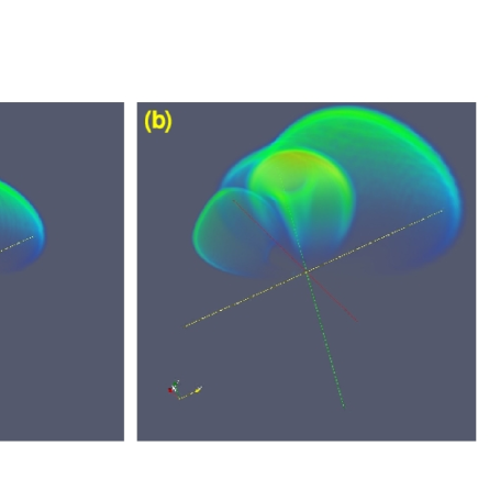
Figure 7: (a) Three-dimensional reconstruction of the two 2011 March 7 CMEs, with CME1 on the left, and CME2 on the right. The ecliptic plane is the xy-plane. The central ejecta of both CMEs is modeled with a flux rope shape. For CME2, the shape of the shock ahead of the flux rope is also modeled. The reconstruction corresponds to a time of UT 21:40 on March 7, by which time the leading edge of CME2 is just entering the HI1-A field of view. (b) Similar to (a), but corresponding to a later time of UT 5:10 on March 8, when CME2 has advanced a little more than halfway through the HI1-A field of view. The faster CME2 has caught up with CME1, and the CME2 shock has been deformed by the solar wind velocity gradient across the longitudinal extent of the shock.

We use these procedures to reconstruct the 3-D morphology of the two 2011 March 7 CMEs, with Figure 7 showing the result. Figure 7a shows the CMEs at 21:40 UT on March 7, before the CME2 FR has decelerated very much. By the time of Figure 7b (at 5:10 UT on March 8) CME2 has caught up with CME1, but it has also decelerated to a speed not much higher than that of CME1 (see Figure 6), so further propagation outwards does not yield much additional motion of the CMEs relative to each other. There is only a modest amount of overlap between the two CMEs in the reconstruction, but this region of overlap happens to be directed towards Earth (see Figure 2). The FR of CME1 is a very fat one, with a highly elliptical cross section. The trajectory of the center of the flux rope is directed $22^{\circ}$ north and $27^{\circ}$ east (e.g., N22E27) of the Sun-Earth line. The west leg of the FR is tilted $45^{\circ}$ above an east-west orientation. For CME2, the FR is directed towards N35W28, with a west leg tilted $75^{\circ}$ below an east-west orientation.

Simple, self-similar expansion is assumed for the FR components of the two CMEs. Such is not the case for the CME2 shock, however. The asymmetric and time-dependent behavior of the shock morphology has already been described qualitatively in section 2. Within the framework of our model, the shock is initially assumed to be a symmetric, lobular front, as shown in Figure 7a, with a trajectory $25^{\circ}$ degrees from that of the CME2 FR, at N45W58 relative to the Sun-Earth line. However, about 5 hours after the start of the CME, while it is in the HI1-A field of view and the CME is decelerating, we allow a discontinuity to develop in the shock front. The western part of the shock headed towards STEREO-A, associated with front F1 in Figure 4, is allowed to expand outwards farther than the eastern part of the shock headed towards Earth, associated with front F2. We experiment with different degrees of asymmetry, and different longitudinal locations for the discontinuity. We settle on a shock extent 1.35 times greater for the western part of the shock than for its eastern part, with the discontinuity at a longitude of W48 relative to Earth. The resulting shock shape is shown in Figures 2 and 7b.

Synthetic images computed from the 3-D reconstruction are shown in the left panels of Figures 3 and 4. These are computed from the model density cubes using full 3-D Thomson scattering calculations (Billings, 1966; Thernisien et al., 2006; Wood & Howard, 2009), and are displayed in the figures in running difference format, consistent with the real images. Some random noise has been added to the synthetic images for aesthetic purposes, to better match the appearance of the images. It is worth emphasizing that when converging on the best possible model parameters, all STEREO and LASCO images are considered, not just the select few we can show in Figures 3 and 4.

The synthetic HI2-A image in Figure 4 shows how the shock discontinuity in the model does yield two distinct fronts (F1 and F2) in the synthetic image. This resembles the shock’s appearance in the real image, although the agreement between the synthetic and real images is far from perfect. For one thing, the model shock clearly extends too far to the south. Improving matters would presumably require making the shock even more asymmetric than it already is, but there is a limit to the shapes that can be made with the parametrized functional forms we are using for FR and shock shape modeling.

The reconstructed shock shape is not only designed to approximate the shape of the shock in the images, but also to reproduce the arrival time of the shock observed at Wind and STEREO-A. This means we need to know precisely the shock kinematics specifically towards Earth and STEREO-A, and Figure 6 explicitly shows the kinematic profiles of the shock in those directions. Towards Earth, the shock distance is smaller than the top of the FR because Earth and Wind are being hit by the flank of the shock (see Figure 2). Since self-similar expansion applies to this part of CME2, this means that the shock velocity towards Earth is proportionally slower as well. Towards STEREO-A, the kinematics are somewhat more complicated because of the shock discontinuity that is allowed to develop while CME2 is decelerating. Figure 6 shows the kinematic profile that results from this discontinuity. Mostly because of the factor of 1.35 increase in shock radial extent, the shock speed at STEREO-A is almost 400 km s^-1 faster than at Earth. Thus, the shock arrives much earlier at STEREO-A than at Wind, as observed.

The top panel of Figure 5 shows the density profiles predicted by the model at Wind and STEREO-A. The density peaks associated with the shock agree with the observed arrival time of the shock to within a couple hours. As mentioned in section 2, at Earth there is geoeffective CME ejecta observed after the shock. Our reconstruction shows a broad density peak after the CME2 shock at Wind, consistent with this. Inspection of Figure 2 reveals that this material is not from CME2 but from CME1. The reconstruction suggests that after the CME2 shock strikes Earth, there is then a glancing blow from the FR component of CME1. Since it is such a grazing incidence, and because the CME2 FR is also not too far away from the Sun-Earth line, confidence in this conclusion is not high, but we do find it more likely that the CME1 FR accounts for the geoeffective ejecta than the CME2 FR. In this interpretation, the density peak seen by Wind at the end of March 10 would be CME1 material that had been shocked by the CME2 shock when CME2 overtakes CME1 shortly after CME2 enters the HI1-A field of view.

Figure 1 shows the inferred trajectories of the various components of CME1 and CME2 relative to their source regions. The CME1 FR is directed somewhat northeast of AR1166, which is where the flare associated with the CME occurs. This trajectory is consistent with the EUV observations of the event from the Solar Dynamics Observatory (SDO), which show that the EUV dimming associated with the eruption is mostly north of AR1166. The CME2 FR ends up directed about $15^{\circ}$ to the east of its source region, AR1164. This eastward deflection is probably caused by the coronal hole to the west of AR1164. Gopalswamy et al. (2009) provide many examples of CME ejecta that are deflected away from coronal holes, demonstrating that this is a common effect. In contrast, the shock expands readily into the fast outflow from the coronal hole. A faster lateral propagation speed through the coronal hole is possibly indicative of higher Alfvén speeds in and above the coronal hole, compared to elsewhere.

5 SHOCK NORMAL MEASUREMENTS

We have associated the March 10 shock observed by Wind with the CME2 shock, but this interpretation is not definite considering the close proximity of CME1, and considering that Earth is near the eastern edge of the CME2 shock. We can search for support for the CME2 association by using the in situ data and the hydromagnetic Rankine-Hugoniot (RH) jump conditions (e.g., Shu, 1992) to infer the shock normal at Wind. The CME2 shock as reconstructed here is centered north of the ecliptic plane, and well to the west of the Earth. Thus, the shock normal at Earth is expected to be in a southeasterly direction. This is the prediction that we intend to test.

It is possible to estimate a shock normal solely from the magnetic field and/or velocity measurements using the coplanarity properties of the RH equations (Colburn & Sonett, 1966; Abraham-Schrauner, 1972). However, these techniques do not work well for all possible shock geometries. They also do not consider all possible constraints on the problem, involving all relevant plasma measurements and the full set of RH equations. Increasingly sophisticated computation techniques have since been developed to more precisely determine shock normal characteristics from single spacecraft measurements (Lepping & Argentiero, 1971; Viñas & Scudder, 1986; Szabo, 1994; Koval & Szabo, 2008).

We have developed our own computational tools to evaluate the normal of the CME2 shock, which closely resembles the prescription of Koval & Szabo (2008, hereafter KS08). We refer the reader to that paper for a full list of the relevant RH equations. The jump conditions are generally expressed as six separate equations, but in practice there are eight, since the equations expressing conservation of tangential momentum flux and tangential electric field are vector equations that can each be decomposed into two scalar equations, for vector components parallel and perpendicular to the shock front (see, e.g., Lepping & Argentiero, 1971). Utilizing these eight equations requires pre- and post-shock measurements of eight quantities: density, temperature (or pressure), vector velocity, and vector magnetic field.

Figure 8 displays these eight quantities for the CME2 shock, both at STEREO-A and at Wind. The data are shown with 1 minute time resolution. Time intervals of about 20 minutes duration are used to assess the pre- and post-shock plasma state. For each plasma quantity an initial mean and standard deviation are computed within the interval. We then throw out points more than 1.5 standard deviations from the mean to exclude particularly anomalous excursions. We then recompute the mean and standard deviation, and the resulting values are illustrated with horizontal lines in Figure 8.

The RH equations apply only in the rest frame of the shock, so the velocity and field components measured in Figure 8 must be rotated into the shock frame before numbers can be plugged into the RH equations. This requires the assumption of a shock normal ($\phi$,$\theta$), and a shock velocity normal to the shock ($V_{S}$). The goal as described by KS08 is to systematically explore the three-dimensional parameter space described by ($\phi$,$\theta$,$V_{S}$) to assess where the RH conditions are most precisely met. Our approach is similar, but rather than keep $V_{S}$ as a free parameter, we instead compute it from the radial shock speed measured in the STEREO images, $V_{rad}$. Figure 6b indicates that $V_{rad}=991$ km s^-1 at STEREO-A, and $V_{rad}=617$ km s^-1 at Wind. If ($\phi$,$\theta$) are defined in a spacecraft-centered RTN coordinate system, then

$$V_{S}=V_{rad}\cos{\phi}\cos{\theta}$$ (3)

Thus, in practice our parameter space is just two-dimensional, defined only by the shock normal ($\phi$,$\theta$).

Each of the eight jump conditions, $X_{i}$ (i=1-8), can be written as

$$X_{i}=\mbox{[pre-shock state]}-\mbox{[post-shock state]}=0.$$ (4)

So for a given ($\phi$,$\theta$) normal we can plug the numbers into each equation and see how close each equation is to zero. However, assessing how well $X_{i}$ are approximating zero requires uncertainties to be computed for each $X_{i}$. We do this using Monte Carlo simulations, where the 8 pre-shock and 8 post-shock measurements illustrated in Figure 8 are varied in a manner consistent with the displayed mean and standard deviation. We also vary $V_{rad}$ in the simulations, assuming 5% uncertainties in our measurements of this parameter. For each trial, we compute a value of $X_{i}$ and after all trials are complete we then compute the standard deviation of these values, $\sigma_{i}$. We can then compute a $\chi^{2}$ number (Bevington & Robinson, 1992) to quantify how well each assumed shock normal is collectively fitting the RH conditions:

$$\chi^{2}(\phi,\theta)=\sum\limits_{i=1}^{8}\left[\frac{X_{i}(\phi,\theta)}{\sigma_{i}(\phi,\theta)}\right]^{2}.$$ (5)

The best fit normal is simply where the $\chi^{2}$ array has its minimum value of $\chi^{2}_{min}$. If we define $\Delta\chi^{2}=\chi^{2}-\chi^{2}_{min}$, then contour plots of $\Delta\chi^{2}(\phi,\theta)$ can be used to define confidence intervals for $\phi$ and $\theta$.

We validate our shock normal computation code using the same synthetic shocks created by KS08 to validate their routine. The one significant difference between our approach and that of KS08, besides the treatment of $V_{S}$ as a measured rather than a free parameter, is that KS08 do not explicitly measure pre- and post-shock plasma parameters (and uncertainties) but instead plug sets of measurements for specific pre- and post-shock times into the RH equations, considering all pre- and post-shock times within some time interval to do their version of our Monte Carlo simulations. We experimented with a version of our code that performs the calculation in this manner, and we did not find any dramatic difference in results for the CME2 shock studied here.

In Figure 9, we show the $\Delta\chi^{2}$ contours for the CME2 shock at both STEREO-A and Wind. Following common practice, we draw contours corresponding to probabilities associated with the 1-, 2-, and 3-$\sigma$ levels of a normal distribution, which are 68.3%, 95.4%, and 99.7% confidence levels. For STEREO-A, the best fit has $\chi^{2}_{min}=1.24$. Interpreting this number requires knowledge of the degrees of freedom, $\nu$, which in this case is $\nu=6$, i.e., eight jump conditions minus two free parameters. Thus, the reduced chi-squared, $\chi^{2}_{\nu}=\chi^{2}_{min}/\nu=0.21$, somewhat below the expectation value of 1 (Bevington & Robinson, 1992). Consultation with a chi-squared probability table (or direct computation of the distribution) reveals that for $\nu=6$, $\chi^{2}_{min}=1.24$ corresponds to a probability value of $p=0.97$, meaning there is a 97% chance that the measured parameter uncertainties illustrated in Figure 8 can explain the magnitude of $\chi^{2}_{min}$. One consequence of the low $\chi^{2}_{min}$ value is that the confidence intervals are rather large for STEREO-A in Figure 9.

In contrast, for the shock at Wind, $\chi^{2}_{min}=8.00$, corresponding to $\chi^{2}_{\nu}=1.33$ and $p=0.24$. A 24% chance that the assumed uncertainties can account for the magnitude of $\chi^{2}_{min}$ is still high enough to consider this a reasonably good fit, although the low value might indicate that the uncertainties in Figure 8 may be a little too low. The confidence contours are naturally much tighter for Wind in Figure 9 than for STEREO-A.

For STEREO-A, we find a shock normal of ($\phi$,$\theta$)=($-31^{\circ}\pm 14^{\circ}$, $-43^{\circ}\pm 10^{\circ}$), while for Wind we find ($\phi$,$\theta$)=($-59^{\circ}\pm 5^{\circ}$, $-28^{\circ}\pm 6^{\circ}$). The quoted 1-$\sigma$ uncertainties are estimated not from the $\Delta\chi^{2}$ contours, but from Monte Carlo simulations where we vary the measurements illustrated in Figure 8 in a manner consistent with the displayed mean and standard deviation, perform the analysis just described, and after many trials the standard deviations of the resulting best fit ($\phi$,$\theta$) values provides the 1-$\sigma$ uncertainties in ($\phi$,$\theta$). We find that uncertainties estimated in this direct manner are larger than those estimated from the $\Delta\chi^{2}$ contours, possibly due to nonnormal characteristics of the uncertainties in this particular problem (Press et al., 1989).

Both normals are south-directed (i.e., negative $\theta$), which is what we would expect given the northward direction of the CME2 shock. At STEREO-A, the shock may be oriented somewhat towards the east (i.e., negative $\phi$), which is not necessarily expected, but uncertainties in $\phi$ are fairly high for STEREO-A. Most importantly, the Wind analysis indicates that the shock there is highly oriented towards the east (i.e., negative $\phi$), consistent with expectations for the CME2 shock, and not consistent with a CME1 association. This provides strong support for the Mar. 10 shock at Wind indeed being the CME2 shock.

In passing, we note that about 10 hours before the CME2 shock hits STEREO-A, it encounters the Venus Express spacecraft at Venus. The location of Venus is shown in Figure 2. A quick coplanarity analysis (Colburn & Sonett, 1966) based only on the magnetic field data yields ($\phi$,$\theta$)=($-57^{\circ}$, $-48^{\circ}$), reasonably consistent with our measurements at STEREO-A, but with an even more eastward orientation, which as mentioned above would not be easy to explain.

6 MHD MODELING

Sophisticated 3-D MHD modeling codes are becoming increasingly useful for modeling the solar wind and transients within it. Models of this sort include the ENLIL code currently being used as an operational space weather modeling tool at NOAA’s Space Weather Prediction Center (Odstrcil & Pizzo, 1999, 2009), and the Space Weather Modeling Framework (SWMF) package (Tóth et al., 2005). We here test whether this sort of modeling can reproduce the general asymmetric shape of the CME2 shock inferred from the empirical reconstruction. The model of Riley et al. (1997) already demonstrates an ability to produce shock asymmetries of this sort due to solar wind inhomogeneities.

The code we use here is a well established model described most extensively by Wu et al. (2007a, b), which has been used to confront STEREO data before (Wood et al., 2011; Wu et al., 2011). This model combines the Hakamada-Akasofu-Fry (HAF) code (version 2; Fry et al., 2001), which computes the solar wind’s evolution out to 18 R_⊙, and a fully 3-D MHD code that then carries the simulation out to 285 R_⊙ (Han et al., 1988). The inner boundary conditions for the HAF part of the code are derived from solar magnetograms and resulting source surface maps using the Wang-Sheeley-Arge model (Wang & Sheeley, 1990; Arge & Pizzo, 2000). This establishes the ambient solar wind into which CME2 is launched. In the model a CME front is produced by introducing a velocity pulse at the inner boundary.

For various reasons, the HAF code cannot properly model the lateral propagation of a CME disturbance into an adjacent coronal hole. For one thing, the HAF code is essentially a 1-D radial propagation model, rather than a 3-D code. For another, the piston used to initiate a fast CME like CME2 is a very large one, which means that part of the velocity pulse extends into the coronal hole right from the start, even if its center is outside the hole. Truly modeling the propagation of a CME front into a coronal hole would probably require a full 3-D MHD model with a lower inner boundary than ours, a smaller piston, and with a higher spatial resolution than we are using.

However, the existing model described above should still be able to study shock asymmetries induced by radial propagation into an inhomogeneous medium. Since the early lateral propagation effects cannot be modeled properly, we place the piston at the empirically inferred center of the shock (N45W58) right from the start rather than at the FR location (N35W28), where the driver is really located. As in past models (e.g., Wu et al., 2007a, b), the velocity pulse is Gaussian-shaped, with the velocity of the piston decreasing with angular distance from piston-center. The width of the piston is described by the Gaussian $\sigma$ parameter (Hakamada & Akasofu, 1982), which in this case is $\sigma=80.2^{\circ}$. Temporally, the velocity pulse consists of a 140 minute exponential rise in velocity up to a maximum speed of 1550 km s^-1 at piston-center, followed by a 140 minute fall back to the original ambient solar wind speed. This leads to a compression wave that arrives at both STEREO-A and Earth near CME2’s actual observed time of arrival at those locations.

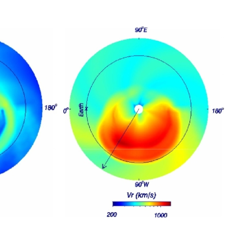
Figure 10: Maps of density (left) and velocity (right) in the ecliptic plane, computed from an MHD model of CME2. The model CME front is shown at a time of 6:00 UT on 2011 March 9, as the CME2 shock approaches 1 AU at STEREO-A’s position $87.6^{\circ}$ west of Earth. The arrows indicate the central longitude of the piston used to initiate the CME in the model.

Figure 10 shows the shape of the modeled disturbance as it approaches 1 AU. Although the model does not precisely reproduce the empirically inferred shock shape in Figure 2, at least qualitatively, the CME front exhibits the same sort of asymmetry inferred for the CME2 shock, being much farther from the Sun west of the piston longitude, where fast solar wind predominates, compared to east of the piston location, where slow wind predominates. This is encouraging for ongoing attempts to explore how these kinds of MHD models can be used to improve CME arrival time forecasts at 1 AU.

7 SUMMARY

We have empirically reconstructed the morphology of two CMEs from 2011 March 7, denoted CME1 and CME2, with a particular focus on the shape of the shock produced by the faster CME2. The location of CME2 in between Earth and STEREO-A, with a shock broad enough to hit both, allows us to bring an extensive collection of observations to bear on assessing the characteristics of the event, involving both imaging and in situ data. Our findings are summarized as follows:

1.

A coronal hole to the west of CME2’s source location has noticeable effects on both the flux rope driver of the CME, which is deflected to the east away from the hole, and the shock front, which in contrast to the flux rope expands more readily over and above the coronal hole. Visual evidence for the shock asymmetry induced by the presence of the coronal hole is apparent in both coronagraphic and heliospheric images of the CME shock.

2.

In situ data also provide evidence for CME2 shock asymmetries induced by the coronal hole, as the shock is observed to arrive at STEREO-A over a day before being observed by Wind near Earth. We use the in situ measurements and the Rankine-Hugoniot shock jump conditions to measure the shock normals at STEREO-A and Wind. The orientations of the shock normals in both locations are in reasonably good agreement with what is expected on the basis of the shock morphology inferred from the STEREO images.

3.

The asymmetries inferred for the CME2 shock are qualitatively reproduced by an MHD model of the CME, which clearly shows the shock expanding radially more rapidly in regions of high speed wind.

4.

After the CME2 shock hits Wind, CME ejecta is also observed that produces a modest geomagnetic storm at Earth. Based on our empirical reconstruction, we tentatively attribute this material not to CME2 but to CME1, which would imply that this is CME1 ejecta that was shocked by the CME2 shock close to the Sun.

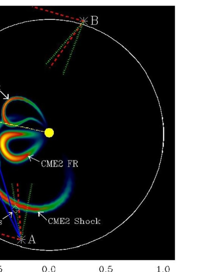
Figure 2: Ecliptic plane map at the time of the two 2011 March 7 CMEs, in heliocentric aries ecliptic coordinates. A slice through the 3-D reconstruction of the two CMEs (see section 4) is shown, indicating the locations of the flux rope (FR) components of CME1 and CME2, and the location of the CME2 shock. Dotted and dashed lines illustrate the fields view of the HI1 and HI2 telescopes on the two STEREO spacecraft. The lines labeled F1 and F2 indicate two tangent points to the CME2 shock as viewed from STEREO-A, which correspond to two separate fronts seen in HI2-A images.

Figure 6: (a) Kinematic model for CME1. The top panel shows measurements of the distance of the top of the CME1 flux rope from Sun-center as a function of time. These measurements are fitted with the simple three-phase kinematic model described in the text, yielding the solid line fit to the data, and the velocity profile shown in the bottom panel. (b) Same as (a), but for the leading edge of the CME2 flux rope. The dashed line indicates the inferred kinematic behavior of the part of the CME2 shock headed towards STEREO-A, and the dot-dashed line shows the kinematic profile of the part of the shock headed towards Earth.

Figure 8: In situ observations of the CME2 shock at both STEREO-A and Wind. From top to bottom the quantities are proton density, temperature, three components of velocity, and three components of magnetic field. The velocity and field components are for an RTN coordinate system. Dotted lines indicate time ranges used to measure pre- and post-shock plasma parameters. These measurements and their uncertainties are shown as horizontal solid and dashed lines, respectively.

Figure 9: Shock normals relative to the Sun-observer axis, computed for the CME2 shock at STEREO-A (left) and Wind (right), based on the plasma measurements in Figure 8 and the Rankine-Hugoniot shock jump conditions. Diamonds indicate the best fit, with surrounding 68.3%, 95.4%, and 99.7% confidence intervals.

References

- Abraham-Schrauner (1972) Abraham-Schrauner, B. 1972, J. Geophys. Res., 77, 736
- Acuña et al. (2008) Acuña, M. H., Curtis, D., Scheifele, J. L., Russell, C. T., Schroeder, P., Szabo, A., & Luhmann, J. G. 2008, Space Sci. Rev., 136, 203
- Arge & Pizzo (2000) Arge, C. N., & Pizzo, V. 2000, J. Geophys. Res., 105, 10465
- Billings (1966) Billings, D. E. 1966. A Guide to the Solar Corona (New York: Academic Press)
- Bevington & Robinson (1992) Bevington, P. R., & Robinson, D. K. 1992, Data Reduction and Error Analysis for the Physical Sciences (New York: McGraw-Hill)
- Bothmer & Schwenn (1998) Bothmer, V., & Schwenn, R. 1998, Ann. Geophys., 16, 1
- Brueckner et al. (1995) Brueckner, G. E, et al. 1995, Sol. Phys., 162, 357
- Burlaga (1988) Burlaga, L. F. 1988, J. Geophys. Res., 93, 7217
- Chen et al. (1997) Chen, J., et al. 1997, ApJ, 490, L191
- Colburn & Sonett (1966) Colburn, D. S., & Sonett, C. P. 1966, Space Sci. Rev., 5, 439
- Eyles et al. (2009) Eyles, C. J., et al. 2009, Sol. Phys., 254, 387
- Fry et al. (2001) Fry, C. D., Sun, W., Deehr, C. S., Dryer, M., Smith, Z., Akasofu, S. -I., Tokumaru, M., & Kojima, M. 2001, J. Geophys. Res., 106, 20985
- Galvin et al. (2008) Galvin, A. B., et al. 2008, Space Sci. Rev., 136, 437
- Gibson & Low (1998) Gibson, S. E., & Low, B. C. 1998, ApJ, 493, 460
- Gopalswamy et al. (2009) Gopalswamy, N., Mäkelä, P., Xie, H., Akiyama, S., & Yashiro, S. 2009, J. Geophys. Res., 114, A00A22
- Hakamada & Akasofu (1982) Hakamada, K., & Akasofu, S. -I. 1982, Space Sci. Rev., 31, 3
- Han et al. (1988) Han, S. M., Wu, S. T., & Dryer, M. 1988, Comput. Fluids, 16, 81
- Howard et al. (2008) Howard, R. A, et al. 2008, Space Sci. Rev., 136, 67
- Kahler & Webb (2007) Kahler, S. W., & Webb, D. F. 2007, J. Geophys. Res., 112, A09103
- Kaiser et al. (2008) Kaiser, M. L., Kucera, T. A., Davila, J. M., St. Cyr, O. C., Guhathakurta, M., & Christian, E. 2008, Space Sci. Rev., 136, 5
- Koval & Szabo (2008) Koval, A., & Szabo, A. 2008, J. Geophys. Res., 113, A10110 (KS08)
- Krall (2007) Krall, J. 2007, ApJ, 657, 559
- Lepping & Argentiero (1971) Lepping, R. P., & Argentiero, P. D. 1971, J. Geophys. Res., 76, 4349
- Lepping et al. (1990) Lepping, R. P., Jones, J. A., & Burlaga, L. F. 1990, J. Geophys. Res., 95, 11957
- Lugaz et al. (2011) Lugaz, N., Roussev, I. I., & Gombosi, T. I. 2011, Adv. Space Res., 48, 292
- Lugaz et al. (2009) Lugaz, N., Vourlidas, A., & Roussev, I. I. 2009, Ann. Geophys., 27, 3479
- Luhmann et al. (2008) Luhmann, J. G., et al. 2008, Space Sci. Rev., 136, 117
- Manchester et al. (2004) Manchester, W. B., Gombosi, T. I., Roussev, I., De Zeeuw, D. L., Sokolov, I. V., Powell, K. G., Tóth, G, & Opher, M. 2004, J. Geophys. Res., 109, A01102
- Marubashi (1986) Marubashi, K. 1986, Adv. Space Res., 6, 335
- Odstrcil & Pizzo (1999) Odstrcil, D., & Pizzo, V. J. 1999, J. Geophys. Res., 104, 28225
- Odstrcil & Pizzo (2009) Odstrcil, D., & Pizzo, V. J. 2009, Sol. Phys., 259, 297
- Press et al. (1989) Press, W. H., Flannery, B. P., Teukolsky, S. A., & Vetterling, W. T. 1989, Numerical Recipes (Cambridge: Cambridge University Press)
- Riley et al. (1997) Riley, P., Gosling, J. T., & Pizzo, V. J. 1997, J. Geophys. Res., 102, 14677
- Sheeley et al. (2008) Sheeley, N. R., Jr., et al. 2008, ApJ, 675, 853
- Shu (1992) Shu, F. S. 1992, The Physics of Astrophysics, Vol. 2: Gas Dynamics (Mill Valley: University Science Books)
- Szabo (1994) Szabo, A. 1994, J. Geophys. Res., 99, 14737
- Thernisien et al. (2006) Thernisien, A. F. R., Howard, R. A., & Vourlidas, A. 2006, ApJ, 652, 763
- Tóth et al. (2005) Tóth, G., et al. 2005, J. Geophys. Res., 110, A011126
- Viñas & Scudder (1986) Viñas, A. F., & Scudder, J. D. 1986, J. Geophys. Res., 91, 39
- Wang & Sheeley (1990) Wang, Y. -M., & Sheeley, N. R., Jr. 1990, ApJ, 355, 726
- Wood & Howard (2009) Wood, B. E., & Howard, R. A. 2009, ApJ, 702, 901
- Wood et al. (2010) Wood, B. E., Howard, R. A., & Socker, D. G. 2010, ApJ, 715, 1524
- Wood et al. (2011) Wood, B. E., Wu, C. -C., Howard, R. A., Socker, D. G., & Rouillard, A. P. 2011, ApJ, 729, 70
- Wu et al. (2011) Wu, C. -C., Dryer, M., Wu, S. T., Wood, B. E., Fry, C. D., Liou, K., & Plunkett, S. 2011, J. Geophys. Res., 116, A12103
- Wu et al. (2007a) Wu, C. -C., Fry, C. D., Dryer, M., Wu, S. T., Thompson, B., Liou, K., & Feng, X. S. 2007a, Adv. Space Res., 40, 1827
- Wu et al. (2007b) Wu, C. -C., Fry, C. D., Wu, S. T., Dryer, M., & Liou, K. 2007b, J. Geophys. Res., 112, A09104
- Wu et al. (2001) Wu, S. T., Andrews, M. D., & Plunkett, S. P. 2001, Space Sci. Rev., 95, 191