†umut.gursoy@cern.ch
‡pgs8b@virginia.edu
On the Temperature Dependence of the Shear Viscosity and Holography
Abstract
We examine the structure of the shear viscosity to entropy density ratio in holographic theories of gravity coupled to a scalar field, in the presence of higher derivative corrections. Thanks to a non-trivial scalar field profile, in this setup generically runs as a function of temperature. In particular, its temperature behavior is dictated by the shape of the scalar potential and of the scalar couplings to the higher derivative terms. We consider a number of dilatonic setups, but focus mostly on phenomenological models that are QCD-like. We determine the geometric conditions needed to identify local and global minima for as a function of temperature, which translate to restrictions on the signs and ranges of the higher derivative couplings. Finally, such restrictions lead to an holographic argument for the existence of a global minimum for in these models, at or above the deconfinement transition.
I Introduction
Over the past decade holography has emerged as a valuable tool for gaining insight into the physics of strongly coupled gauge theories. Top-down studies based on string/M-theory setups have been met by a number of bottom-up constructions, with applications ranging from the realm of quantum chromodynamics (QCD) to that of condensed matter systems. Holographic techniques have been particularly useful for probing the hydrodynamic regime of strongly interacting thermal field theories, a regime which is notoriously difficult to study directly and – unlike thermodynamics – poses a challenge to lattice simulations.
Within this program, many efforts have been directed at better understanding the dynamics of the strongly coupled QCD quark-gluon plasma (QGP), and in particular at computing its transport coefficients. One of the most exciting results which has emerged from the heavy ion program at RHIC – and now at LHC – is the observation that the hot and dense nuclear matter produced in the experiments displays collective motion. In fact, the QGP fireball created in off-central collisions is not azimuthally symmetric, but rather shaped like an ellipse. As a result, the pressure gradients between its center and its edges vary with angle, giving rise to an anisotropic particle distribution. The matter formed in the collisions then responds as a strongly coupled fluid to the differences in these pressure gradients, displaying a collective flow which is well described by nearly ideal hydrodynamics with a very small ratio of shear viscosity to entropy density .
Experimentally, the flow pattern can be quantified by Fourier decomposing the particles’ angular distribution. In particular, it is the second Fourier component , the so-called elliptic flow, which is the largest in non-central collisions and is the observable most directly tied to the shear viscosity. Thus, bounds on can be extracted from elliptic flow measurements, with the most advanced analysis at the moment giving Song:2010mg . Higher order harmonics – initially neglected because they were assumed to be too small for symmetry reasons – also play an important role in determining the shear viscosity (see Section IV for a more detailed discussion). We refer the reader to Teaney:2003kp ; Luzum:2008cw for some early references on the RHIC results and the range of , and to Luzum:2010ag ; Nagle:2011uz ; Shen:2011eg ; Muller:2012zq for more recent ones including discussions of the first LHC results.
A remarkable result that has emerged from holographic studies of strongly coupled gauge theories has been the universality of the shear viscosity to entropy ratio Policastro:2001yc ; Buchel:2003tz , which was shown to take on the particularly simple form in any gauge theory plasma with an Einstein gravity dual description111An exception is the case of anisotropic fluids, as first observed in Erdmenger:2010xm .. Its order of magnitude agreement with RHIC (and now LHC) data was one of the driving motivations behind the efforts to apply holography to the transport properties of the QGP (see CasalderreySolana:2011us ; Adams:2012th for recent reviews). It is by now well understood that deviations from the universal result (both below and above) are generic once curvature corrections to the leading Einstein action are included222For reviews of the shear viscosity bound we refer the reader to Sinha:2009ev ; Cremonini:2011iq ; Banerjee:2011tg .. Moreover, when there is another scale in the system in addition to temperature , the viscosity to entropy ratio typically runs as a function of in such higher derivative theories. We should emphasize that this type of temperature flow for the shear viscosity arises in a number of holographic constructions, from theories of higher derivatives in the presence of a chemical potential Cai:2008ph ; Myers:2009ij ; Cremonini:2009sy or non-trivial scalar field profiles333Dilatonic couplings to higher derivative terms in the context of have also been studied in Cai:2009zv . Cremonini:2011ej ; Buchel:2010wf and also to systems with spatial anisotropy Ghodsi:2009hg ; Erdmenger:2010xm ; Basu:2011tt ; Erdmenger:2011tj ; Rebhan:2011vd ; Oh:2012zu ; Mamo:2012sy .
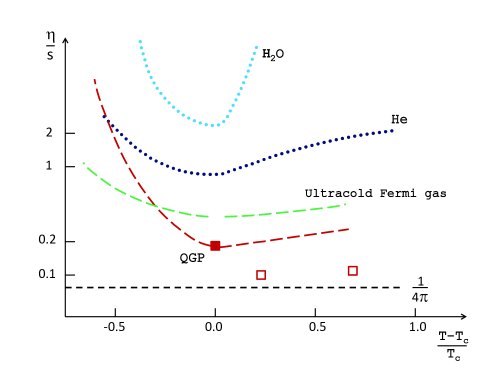
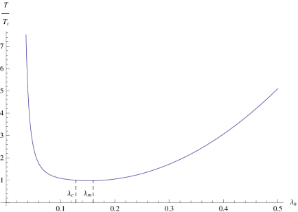
The viscosity to entropy ratio is in fact known to be temperature dependent for a variety of liquids and gases in nature (as well as for ultracold fermionic systems close to the unitarity bound), exhibiting a minimum in the vicinity of a phase transition (see Figure 1). A similar behavior is expected Csernai:2006zz for near the temperature of the QCD phase transition which separates hadronic matter from the QGP phase. In the hadronic phase below , the hadronic cross section decreases as the temperature is lowered, leading to an increase in Gavin:1985ph ; Prakash:1993bt (for an analysis of transport in the hadronic phase see e.g. NoronhaHostler:2008ju ). On the other hand, in the deconfined phase at temperatures well above , asymptotic freedom dictates that should increase with temperature (the coupling between quarks and gluons decreases logarithmically Arnold:2000dr ; Arnold:2003zc ). From the behavior in these two opposite regimes, we conclude that we should expect a minimum for somewhere in the intermediate range.
A precise determination of the temperature behavior of transport coefficients such as is an important ingredient for understanding the dynamics of the strongly coupled medium produced at LHC and RHIC, and may also help in finding the location of the critical point. However, at the moment most hydrodynamical simulations of the QGP assume that is a constant, and therefore insensitive to temperature. The question of the possible relevance of a temperature-dependent on the collective flow of hadrons in heavy ion collisions has been investigated in a number of studies Niemi:2011ix ; Nagle:2011uz ; Shen:2011kn ; Bluhm:2010qf , which thus far have focused mostly on qualitative effects. The results of Niemi:2011ix seem to indicate that at LHC energies elliptic flow values are sensitive to the temperature behavior of in the QGP phase, but insensitive to it in the hadronic phase (with the results reversed at RHIC energies).
Motivated by the potential sensitivity of elliptic flow measurements to thermal variations of at the energies probed by LHC, here we would like to initiate a systematic study of the flow of the shear viscosity as a function of temperature in the context of holography. In this paper we will restrict our attention to theories with a vanishing chemical potential, described simply by gravity coupled to a scalar field in the presence of higher derivative corrections. Although we will not consider string theory embeddings of these backgrounds, the higher derivative terms we examine are generically expected to show up as corrections to the two-derivative Einstein-scalar action viewed as an effective field theory, and in particular to most effective actions derived from string theory. Moreover, our result for in (18) is completely generic and applicable to any top-down model which contains a truncation to an Einstein-scalar theory.
Thanks to the presence of a non-trivial scalar field profile, the higher derivative terms in our theory will generically generate a temperature flow for the shear viscosity, as already expected from Cremonini:2011ej ; Buchel:2010wf . In particular, the temperature dependence of will be dictated by the shape of the scalar potential and of the couplings of the scalar to the higher derivative interactions. Given an explicit expression for in terms of the latter, it is then straightforward to discuss the existence of local minima for as a function of temperature. As we will see, for potentials which confine quarks at zero temperature it is also possible to determine criteria for the existence of global minima. In particular, the requirements that approaches its high-temperature value from below (dictated from asymptotic freedom) and that the zero-temperature theory is confining, are enough to fix the signs (and ranges) of the couplings of the higher derivative terms, and guarantees the existence of a global minimum for , at or above . Thus, we have been able to give a holographic argument for the existence of a minimum for in this class of models, along with a geometric interpretation for it, complementing existing field-theoretic444The authors of Kovtun:2011np tie a lower bound on the shear viscosity to the validity of second-order hydrodynamics. arguments Kovtun:2011np . Finally, although our analysis will be more general, we will focus mostly on ‘phenomenological’ models engineered to reproduce some of the qualitative and quantitative features of QCD.
The rest of the paper is organized as follows. Section II describes our setup and outlines how to obtain for higher derivative corrections to dilatonic black brane solutions. Our main results are presented in Section III, where we discuss the temperature dependence of in theories with a non-trivial scalar field profile, first by considering a toy model consisting of an exponential scalar potential, then focusing on QCD-like phenomenological models. We also comment on qualitative features of in theories that are confining, and identify generic criteria for the existence of a minimum for as a function of temperature in such setups. We summarize our results in Section IV, where we also comment on the challenges involved with determining more precisely the structure of , and in particular how it flows with temperature.
II Setup
In order to generate a non-trivial temperature dependence for at zero chemical potential we will consider backgrounds with a scalar field coupled to a higher derivative theory of gravity. The action we consider is of the form
| (1) |
under the assumption that the coupling of the higher derivative terms is perturbatively small and is an arbitrary regular function of . For most of the paper we will focus on the exponential case, , however most of the analysis is straightforwardly generalized to arbitrary The dilaton potential is assumed to have either a minimum at some value or a run-away behavior as (as in GK ; GKN ). Although in the above we have only considered the higher derivative correction , this is in fact the only term which contributes to at this order in the derivative expansion. The computation of in theories with higher derivatives has been studied in great detail, and here we review briefly only the relevant aspects555For reviews of higher derivative corrections to and further details of the computation we refer interested readers to Sinha:2009ev ; Cremonini:2011iq ; Banerjee:2011tg and references therein..
II.1 Extracting the Shear Viscosity to Entropy Ratio
In the hydrodynamic approximation to near-equilibrium dynamics, the transport coefficients of a finite temperature plasma can be extracted in a number of ways. The most straightforward method for computing the shear viscosity is based on the Kubo relation
| (2) |
which reduces to the low frequency and zero momentum limits of the stress tensor’s retarded Green’s function. Using the holographic dictionary, the relevant two-point correlation function of the shear stress tensor can be read off from the effective action of a shear metric fluctuation , where we use to denote the radial direction in the bulk. Expanding (1) to quadratic order in the modes , one finds the by now standard666See Buchel:2004di for the original derivation, in the context of corrections. form of the effective action for the shear fluctuation,
| (3) | |||||
where the coefficients encode information about the background solution, and is the generalized Gibbons-Hawking boundary term.
After a number of subtle manipulations, the shear viscosity can be extracted from (3) and reduces Myers:2009ij to the compact expression
| (4) |
evaluated at the horizon radius , showing that it is given entirely in terms of horizon data777The Kubo formula (2) can be shown Iqbal:2008by ; Myers:2009ij to be equivalent to (5) where is the radial-momentum conjugate to . In the low frequency limit (as long as the boundary theory is spatially isotropic) the quantity inside the limit does not depend on the radial coordinate. As a result, it can be evaluated at an arbitrary value of , and in particular at the horizon Iqbal:2008by ; Myers:2009ij .. Finally, the entropy density is easily found by dividing by the (infinite) black brane volume Wald’s entropy formula,
| (6) |
where is the induced metric on the horizon cross section , and the binormal to .
From our discussion above it is evident that can be expressed entirely in terms of near-horizon data. Moreover, when working perturbatively in the coupling of the higher derivative terms, can be determined purely from the background solution of the two-derivative theory888Because of the universality of , corrections to the background geometry lead to order corrections to .. These two facts allow us to write in terms of the parameters of a generic near-horizon non-extremal black brane expansion. Parametrizing the black-brane solution to the leading order two-derivative action by
| (7) |
with the choice , we can write down its near-horizon expansion by assuming a first order zero in and a corresponding first order pole in ,
| (8) |
The shear viscosity to entropy density ratio is then of the simple form Cremonini:2011ej
| (9) |
and is only sensitive to the parameters of the near-horizon expansions (II.1). This concludes the derivation of for the theory described by (1). In the remainder of this section we will discuss the class of dilatonic black brane solutions we are interested in.
II.2 Shear Viscosity of Dilatonic Brane Solutions
As we mentioned above, the backreaction of the higher derivative terms on the background solution does not affect to linear order in perturbative parameter , which is the order that we are interested in here. Thus, we are going to focus on black brane solutions to models described by the two-derivative action
| (10) |
and neglect curvature corrections. Although analytic black brane solutions are not known for generic choices of the potential, to extract knowledge of the near-horizon behavior is enough, given our prescription (9). For this calculation we find it more convenient to introduce a new radial coordinate and parametrize the black brane ansatz as
| (11) |
From the expression (9) it is clear that we will need to calculate the near horizon values of the metric functions and in (7), and the relationship between T and , which will make the temperature dependence of (9) explicit. We will instead calculate the near horizon values of the functions and above and perform a change of variables at the end to express (9) in terms of physical quantities.
For this study, it turns out to be particularly convenient to adopt the phase variables method developed in LongThermo , which we briefly review here and in Appendix A. This is a quick and efficient way to obtain the thermodynamic properties of the diatonic branes. In place of solving the full 5th order set of Einstein’s equations, one only needs to solve two first order differential equations for the so-called “phase variables” that are defined from the metric functions as
| (12) |
The constant depends on the normalization of the scalar kinetic term in (1) and dimensionality. In our case it is fixed to be . Clearly, these functions are invariant under reparametrizations of the radial coordinate. Physically, one can interpret the boundary values of these variables as the thermodynamic energy and the enthalpy of the system. Furthermore, their horizon expansion is completely determined in terms of the dilation potential and by the requirement of regularity. The behavior of the metric functions near the horizon is also determined in terms of these two quantities. The details of the calculation are explained in Appendix A and here we present only the final results.
We parametrize the near-horizon expansion of the metric and scalar field of the black brane ansatz (11) at as follows,
| (13) | |||||
| (14) | |||||
| (15) |
We can now make use of the phase variables method to obtain explicit expressions999In particular, we use eqs. (52), (53), (57), (64) and (66) in Appendix A. for and in terms of the physical parameters in the system,
| (16) |
with given by (65). As can be seen from (9), the only near-horizon parameters that are needed for extracting are , the leading order coefficient in the expansion of , and and , the first two terms in the scalar field expansion. By performing a change of radial coordinate we can relate the two near horizon expansions, and write in terms of as
| (17) |
We now have all the ingredients needed to apply the near-horizon prescription (9) to the generic black brane expansion (II.2)–(17) we just found. As expected, we find that the deviation from the universal result is controlled by the shape of the potential, the horizon value of the scalar field as well as the coupling of the higher derivative term,
| (18) |
and for the specific choice of which we will focus on for the most of this paper,
| (19) |
We emphasize that this expression is completely general, and applies to any asymptotically AdS solution to (1). Moreover, we can already anticipate that will generically be temperature dependent, thanks to the presence of a non-trivial scalar field profile, as already seen in Cremonini:2011ej ; Buchel:2010wf . To better understand the meaning of (19), we recall that the flow of as a function of temperature is mirrored, in the bulk, by the change of the near-horizon geometry of the solution, as the horizon radius varies. For the class of holographic constructions we are considering here, it is the scalar field profile which is responsible for introducing an additional scale in the theory (in addition to temperature), and thus breaking the conformal symmetry away from the UV. As a result, we should think of , the horizon value of the dilaton, as tracking the temperature of the system101010More precisely, it will track the dependence on , where is the new scale in the system.. Thus, (19) can be expressed entirely in terms of temperature by finding the precise relationship between and . As usual, the latter can be determined from the metric by demanding regularity at the horizon. We review this is Appendix A.
Finally, we would like to point out that in the special case of a non-dynamical scalar field and a constant potential, we recover the standard result for an AdS black brane in pure gravity with curvature corrections Brigante:2007nu ; Kats:2007mq , which is well-known to give rise to a constant correction to the universal result. More interestingly, there are special choices of non-trivial for which the temperature dependence disappears, as we will see more explicitly below.
III Results
In this section we examine the temperature dependence of in various holographic setups. We start by looking at a toy model consisting of a simple exponential potential, and continue with more ‘phenomenological’ constructions designed to mimic QCD and in particular the physics of the strongly coupled quark gluon plasma. We will conclude by remarking on generic, qualitative features of , including a discussion of the existence of minima as a function of temperature.
III.1 A Warm-up Example: Chamblin-Reall Black Brane
As a warm-up example, we will work out the Chamblin-Reall (CR) black-hole solution CR by making use of the phase variables formalism. The CR brane is a solution to (10) with the single-exponential potential
| (20) |
where is a positive dimensionless constant and defines a length-scale in the background. We choose . With this convention111111In the two-derivative theory, the sign of can be altered by the transformation ., in the zero temperature geometry the scalar approaches on the boundary and in the deep interior. In the black-brane geometry, which is what we are ultimately interested in, runs from on the boundary to a constant value at the horizon. Thus, anywhere outside the horizon .
Although the potential (20) does not admit an AdS minimum as the scalar field approaches the boundary, the CR brane – for a special value of – can be obtained from a dimensional reduction of pure gravity plus a (negative) cosmological constant in six dimensions. In fact our action (1), with the potential choice (20), can be obtained via a reduction from the following six-dimensional mother theory
| (21) |
for the special case121212More general dimensional reductions Gouteraux:2011qh may yield additional values of . of (see Appendix B for details of the reduction). This special parameter choice – for which the CR solution can be uplifted to a pure AdS black brane in six dimensions – will play an interesting role in the behavior of , as we will see later in this section. For now, however, we will keep completely arbitrary.
The CR solution corresponds to the fixed-point of the X-equation (55) with
| (22) |
where recall Substituting this into the Y-equation (56), the solution becomes
| (23) |
From (58) and (59) one can then reconstruct the full background as a function of ,
| (24) |
where corresponds to a cutoff surface, as explained in the appendix. One can now use (62) and (63) to obtain the entropy and temperature as a function of ,
| (25) |
where we defined
| (26) |
The temperature dependence of the entropy can be read off from (25),
| (27) |
Combined with the first law of thermodynamics, this fixes the temperature scaling for the free energy of the system
| (28) |
In both equations (27) and (28) the proportionality constant is positive. Notice that the free energy is always negative definite and never crosses zero – there is no phase transition in the system. Moreover, the requirement that the specific heat of the system is positive definite (for thermal stability) constrains the value of , resulting in . Using (22) this can be translated into a condition on , the exponent in the dilaton potential (20),
| (29) |
Together with this condition, equations (27) and (28) essentially determine all of the thermodynamic properties of the system. The fact that – to work out the thermodynamics associated with this background – we only needed to solve two first order differential equations, (55) and (56), and not the full system of Einstein’s equations, demonstrates explicitly the advantage of using the phase variables method.
We are now ready to calculate the shear viscosity of the CR black-brane solution. Although we are particularly interested in the case of , for which the CR solution comes from a reduction of a pure AdS black brane in six dimensions, here we write down a ‘formal’131313Although our near-horizon prescription was obtained specifically for geometries that are asymptotically AdS, it may be possible to generalize it to backgrounds that contain asymptotically conformally flat radial slices, by appropriately taking into account holographic renormalization in such backgrounds as in Wiseman:2008qa . expression for for arbitrary values of and . Using (20) and the corresponding expressions for the temperature and entropy (25), one finds
| (30) |
Recall from (29) that , and therefore the sign of the power of the temperature in (30) depends on whether or not. In either case, is a monotonic function of the temperature, and whether it decreases or increases relative to depends on the sign of as well as the range of . Furthermore, if we require the zero temperature limit to approach the universal result, we must impose .
Interestingly, the temperature dependence of the shear viscosity to entropy ratio disappears in the two special cases:
-
1.
. In this case not only the -dependence disappears, but also resumes its universal value , despite the presence of higher derivative corrections.
-
2.
. For the special case of takes exactly the same value as in the six-dimensional AdS Schwarzschild black hole. This fact can be understood by reducing the Schwarzschild solution on . It inherits the scale symmetry of the parent solution in six-dimensions, hence leading to absence of the -dependence. See Appendix B for details of this calculation. Similar statements can be made for reductions from -dimensions on an -torus as in Gubser1 , which for would yield .
It is possible that the cancelation of the correction to in the former case may also be understood in terms of a dimensional reduction of a parent theory, but this time without a cosmological constant141414We thank Blaise Gouteraux for a very interesting discussion on this point.. At the moment we don’t have a more complete understanding of this case (see however Blaise ).
III.2 Improved Holographic QCD
III.2.1 ihQCD Background
Next, we turn to the phenomenological models discussed in GK ; GKN ; Gubser1 and focus in particular on the setup of GKMN1 ; LongThermo . These are phenomenological constructions in the sense that the potential is determined purely by field-theoretic requirements, and is designed to capture some of the features of QCD while remaining reasonably tractable. In fact, in these models the dilatonic scalar can be identified151515Up to a multiplicative factor which does not affect physical observables. with the running ’t Hooft coupling, , and the scalar potential is directly related to the -function of the system, giving a holographic definition of the latter in terms of the background geometry. Thanks to this identification one can extract the UV and IR asymptotics of the potential from the small and large expansions of .
In the UV (small ), the input for the behavior of comes from perturbative QCD, i.e. from the requirement of asymptotic freedom with a logarithmic running coupling. More generally, one assumes that there is a dimension-four operator in the spectrum, dual to the dilaton in the bulk. The fact that the operator is marginal in the UV then translates into the statement that the UV geometry is asymptotically , with logarithmic corrections. The details of the UV expansion for these types of backgrounds can be found in GK .
On the other hand, in the IR (large ) the potential is fixed by demanding linear quark confinement. On the bulk side this is implemented by adding a probe string in the geometry – dual to a Wilson-loop – and obtaining the quark-anti quark potential from the asymptotics of the string embedding in the IR Wilson ; GKN . One finds that linear confinement requires the dilaton potential to have an asymptotic expansion in the IR of the form
| (31) |
where we show only the leading large behavior161616The difference between this definition and the original one given in GK arises from different normalizations of the dilaton kinetic term., with and . The parameter choice which fits the available zero and finite temperature data best turns out to be and (see GKMN3 ). This particular choice is also well motivated by the fact that it exhibits desirable qualitative features such as a linear glueball spectrum, screening of the magnetic quarks GKN , and more recently the scaling behavior of the interaction measure in temperature Delta 171717See Veschgini:2010ws and references therein for a criticism of ihQCD models..
More specifically, defining , an example of a potential with the correct UV and IR asymptotics is of the form
| (32) |
where the value at sets the UV AdS scale . The remaining parameters in the potential (32) can be fixed by matching the scheme-independent -function coefficients of large N QCD, the lowest glue ball mass and the latent heat at GKMN3 . Although we will analyze explicitly the model with the potential given in (32), we emphasize that our qualitative results will only depend on the fact that in the UV and that it is a confining potential in the IR.
III.2.2 Thermodynamics
(a)
(b)
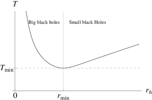
Before discussing the temperature dependence of the shear viscosity in this setup, we would like to summarize the basic thermodynamic properties of the system. These models exhibit a first order confinement-deconfinement transition at some critical temperature . Below , the dominant phase is the confined phase that corresponds to a thermal graviton gas background. On the other hand, above one has the deconfined phase corresponding to a big black-hole background. We note that there also exists a third phase above a certain temperature , where , which is sometimes referred to as a small black-hole. While the horizon of the latter is deep in the interior, the big black hole has its horizon closer to the boundary.
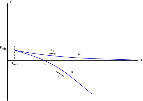
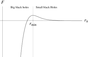
The presence of the two types of black-holes is apparent from Figure 2(a), which shows as a function of the horizon location. It is also clear from the figure that there are no black hole solutions for . Although the small black-hole is always sub-dominant and has a negative specific heat, its presence will turn out to be important to understand certain properties of in the following discussion. Figure 2(b) shows the variation of the free-energy density as a function of the horizon radius. Finally, by combining Figure 2(a) and Figure 2(b) one can parametrically solve for the free energy as a function of temperature. The result is sketched in Figure 3, which also summarizes the phase structure of the system as the temperature is varied.
III.2.3 Shear Viscosity of ihQCD
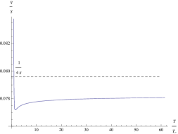
Given the general formula (19) and the dilaton potential (32), it is immediate to obtain as a function of the scalar at the horizon. However, physically one is interested in having as a function of temperature, rather than . Conversion from the latter to temperature is done by using either (62) or (66), after solving Einstein’s equations numerically for the background functions. Figure 4 shows the results of this calculation, for the choice of potential (32) which gives the best fit to the available lattice data GKMN3 .
We note that the behavior of as a function of the horizon location is indeed of the form of Figure 2(a), with the minimum separating the big black hole (on the left) from the small black hole branch (on the right).
Combining with the analytic expression (19) and the potential (32), one can now plot as a function of , for a choice of the parameters and . Unfortunately, we were unable to constrain the possible range of with the available data, but instead chose representative values (recall however that we want to be small enough so that the curvature corrections in (1) remain perturbative). Depending on the choice of the couplings , will then display different qualitative behaviors.
Two interesting fiducial cases – which are representative of the behavior of the viscosity in a large portion of the phase space – correspond to taking , and , .
(a) (b)
In the first case, shown in Figure 5(a), displays a local minimum as a function of which, for the parameter choices made there, appears around . In the high temperature limit approaches the universal value from below. The behavior in the second case, depicted in Figure 5(b), is quite distinct. There increases monotonically with temperature above , increasing indefinitely as , just as in perturbative QCD. There is no local minimum appearing in the range , and therefore acquires its minimum value at . In both cases, we know from field theory studies of the hadronic phase that increases monotonically for , as one probes lower and lower temperatures. Thus, in Figure 5(b) we expect to correspond to the global minimum of the function .
In these two examples, the qualitative behavior of the viscosity is different not only near , but also in the high-T regime. We should note, however, that our holographic results can only be trusted up to a certain , above which the perturbative higher derivative expansion breaks down181818A potentially useful way of characterizing this break-down is by requiring , and evaluating this at the horizon. This yields the relation from which one can compute , corresponding to the point at which the correction becomes . However, making this relation more precise is beyond the scope of this paper.. In particular, we won’t be able to trust an arbitrarily large deviation from the universal result. Other interesting qualitative behaviors are also possible, in the remaining range of . For example, a mixture of the two aforementioned cases arises when and . In this case exhibits a local minimum above just like in the first case above, but its high-T behavior is the same as that of the second case. We will provide a more detailed derivation of the different qualitative features of as a function of temperature in the next section, where we will also discuss the boundaries of the various regions of phase space which lead to the distinct behaviors.
III.3 Qualitative Features of the Shear Viscosity for Confining Backgrounds
We would like to conclude this section by exploring some of the qualitative features of the temperature dependence of from a more general point of view. For concreteness we will restrict our attention to dilaton potentials that exhibit confining IR asymptotics (as ) as in the ihQCD case of the previous section,
| (33) |
and AdS asymptotics in the UV. Furthermore, we will consider the following two possibilities for the behavior of the potential in the UV:
-
a.
as
-
b.
as .
The first case (under the assumption that to ensure AdS boundary conditions) is precisely that of ihQCD-type backgrounds, where the dilaton is massless and corresponds to a marginal deformation by the dimension-four operator . The second case describes a massive dilaton of mass , and corresponds to a deformation of the UV conformal theory by an operator of scale dimension191919Note that the normalization of the kinetic term for our scalar differs by a factor of four from that of more standard AdS/CFT conventions, leading to a slightly different relation between the scalar mass and the conformal dimension of the dual operator.
| (34) |
Thus, relevant deformations correspond to , and the Breitenlohner-Freedman (BF) bound is given by .
In holographic constructions of the type we are considering, the flow of as a function of temperature results from the way in which the near-horizon geometry changes as the horizon radius varies (it comes from sampling the phase space of the possible solutions to the theory). In our setup, the horizon value of the scalar field tracks the temperature of the system. High temperatures then map to in the a) type potentials, and in the b) type potentials we have just discussed, whereas ‘low’ temperatures correspond to the region just above . We emphasize that the geometry which is relevant in this entire temperature range is that of the big black-hole discussed in Section III.2.2. Thus, the high-T behavior of will correspond to the large horizon limit of the big black-hole geometry. Below , the thermal gas phase dominates, and we won’t attempt to compute directly in that regime (we will discuss the subtleties involved with such a calculation towards the end of this section). Instead, we will extract information about the structure of – and in particular any minima it has as a function of temperature – by exploiting the existence of both the big and small black-hole branches. Thus, even though the small black-hole is not of direct physical interest – it is not thermodynamically favored – it is still (indirectly) useful for probing .
We start by working out the viscosity to entropy ratio in the regime which corresponds to the small black-hole branch. In particular, we work in the limit which describes an extremely small horizon radius (the far right of Figure 4). In this regime, we can extract by plugging the IR potential (33) into our general formula (19), which gives
| (35) |
where we are omitting terms that are subleading in the large limit. Given that the small black-hole is not thermodynamically favored, we emphasize that the only crucial piece of information we need to extract from this expression is whether increases or decreases as grows larger and the small black-hole shrinks. We can see from (35) that as grows, the correction to tends to become202020Analysis of the sub-leading terms shows that it becomes large and positive even when . large and positive for and , while it tends into the large and negative direction in the opposite case (assuming in all these cases that ). On the other hand, when the sign of the exponential term changes, and the correction term vanishes in the extreme small black hole limit, from above (below) when the product is positive (negative).
We note that in all of this analysis is assumed to be perturbatively small212121 To ensure the absence of additional degrees of freedom associated with the higher derivative corrections in (1)., . Of course when the higher derivative correction (35) becomes ‘too large,’ the result can no longer be trusted – for consistency one would have to include not only the four-derivative term in the action (1), but all other higher derivative corrections as well. However, our expression for above will still be useful for the following two reasons. First, in many phenomenological potentials of the type we are interested in, the leading IR behavior (33) doesn’t necessarily set in at a very high value of . Thus, in these cases there will be a region of validity for (35), which can be made larger and larger by choosing (or ) smaller. Secondly, as it will become clear below, what we are really after is not the precise value of (35), but rather whether tends upwards or downwards on the small black-hole branch.
Next, we move on to discussing the high-temperature behavior of realized on the big black-hole branch222222We are now probing the near-horizon geometry of the big black-hole solution, in the large horizon limit., which maps to and for type a) and type b) potentials, respectively. We analyze the two types of UV asymptotics for the potential separately. In case a) one finds, for negative and large (the black hole horizon is close to the runaway AdS region)
| (36) |
Thus, in the high- regime attains its universal value, for . Note that it approaches this value from above (below) for (). On the other hand, for , tends upwards (downwards) for (). We note that in the case the result is only trustable up to a certain (negative) value of , above which other higher order derivative corrections should also be taken into account. Thus, the expression for is only reliable up to a certain .
For the b) type potentials, i.e. with a true AdS minimum at , one finds instead
| (37) |
First of all, we learn that takes the value one expects232323This conclusion is independent of the sign of , because of the limit. from a curvature-squared correction (with no dilatonic scalar coupling) in five dimensions Kats:2007mq . Furthermore, recalling that the BF bound is , we see that approaches its constant high- value from above (below) for ().
There are a number of generic qualitative statements one can make about the running of with temperature for these confining backgrounds:
Divergence of :
First, it is known LongThermo that for any potential that confines quarks at zero temperature, there exists a temperature (below ) in the finite temperature theory where the small and big black-hole branches meet, as shown in Figure 2a). This implies that diverges at this point and that is double-valued above . As a result, although itself is finite at , by the chain rule, its derivative will diverge there242424One may worry that a diverging might reflect a regime that can’t be trusted. However, we can keep corrections to arbitrarily small by appropriately tuning the perturbative coupling . More importantly, the divergence of the derivative of at is a result of the double-valued nature of – the quantity itself remains finite and small. Thus, given that we are only interested in qualitative features of – whether it increases or decreases near , and the sign of its slope there – the divergence of is not expected to present a problem.. This is a generic feature of that holds for any holographic background corresponding to a large N confining gauge theory at zero temperature.
This behavior is exemplified in Figures 7 and 8, which show that the divergence occurs at the meeting point of the big and the small black-hole branches. We should note that it is the thermal gas, and not one of the black-hole solutions, that is the thermodynamically preferred solution at this temperature and so the divergence in does not actually correspond to a physical property of the shear viscosity. Even though it cannot be considered a physical characteristic of , knowledge of the divergence of at will prove useful in analyzing the functional properties of In particular, it will provide an holographic explanation for why assumes its minimum value at the transition point for confining gauge theories, as we will see shortly.
There is also a particular case in which the divergence occurs on the border of a thermodynamically dominant branch and, as such, does correspond to a physical property of . As described in LongThermo and G1 , a second order confinement-deconfinement transition corresponds to the case when and coincide. In this situation there is no small black-hole branch, and the derivative of generically diverges precisely at the transition point . More precisely, diverges at and therefore one generically expects that also diverges, as long as remains finite at that point. This latter condition should be analyzed separately.
As a concrete example of this case, we take the generic backgrounds considered in G1 , which exhibit a second (or higher) order Hawking-Page transition at a finite temperature at which . In order to find the behavior of around the transition point, one should first make sure that the perturbative approximation in the higher derivative expansion is valid as . The scalar potential in the theories of G1 has the asymptotic behavior shown in (33) with and , together with exponentially decaying sub-leading terms as ,
| (38) |
Here is a positive constant which does not play any role in the following discussion, and the value of determines the order of the continuous transition.
From the expression (35) we see that we can only make reliable statements about the behavior of the shear viscosity as () in the particular case (otherwise our perturbative approximation is guaranteed to break down). For this choice of parameters one then recovers the universal result as . It is straightforward to work out the behavior of the derivative of by combining and . The first can be calculated straightforwardly from (35). The latter follows from the sub-leading analysis performed in G1 , which gives the following relation between temperature and ,
| (39) |
where . Finally, combining these ingredients one obtains,
| (40) |
where the sign of the proportionality constant is positive (negative) for (). Thus we arrive at the conclusion that, although remains finite and reaches its universal value at the continuous transition, its derivative diverges for , and it vanishes for . We emphasize again that our perturbative approximation breaks down for , in which case one cannot reliably determine the behavior of at . This concludes our aside on the special case in which the divergence occurs on the border of a thermodynamically dominant branch. In the rest of the paper we will assume that .
Conditions for local minima:
Our general expression (19) makes the discussion of the presence or absence of a minimum for straightforward. Local minima are defined by the following two conditions252525Without loss of generality we assume that is finite at these minima.,
| (41) |
which, when re-instating the generic higher derivative coupling , can be translated into analyticity conditions on and the dilaton potential using (19). In particular, extrema of are determined by the locii at which
| (42) |
an expression which is valid for arbitrary potentials (which allow for AdS asymptotics) and scalar couplings , and not just the particular setup of this section. In terms of , the condition becomes
| (43) |
Thus, in order for to have an extremum at a certain temperature, a necessary condition262626This is also sufficient provided that is finite at this point. is that the dilaton potential possesses at least one solution to equation (42). Clearly, for such a solution to correspond to a minimum one should further ensure that the second derivative is positive there. These two conditions provide a simple criterion for the existence of extrema, given an arbitrary scalar field profile in the class of theories (1).
Presence of a global minimum:
The discussion in the previous paragraph concerns general conditions for the existence of local minima. However, we can also ask what are the conditions for the existence of a global minimum, given a confining potential with the IR and UV asymptotics described above. To answer this question, it turns out to be useful to recall the behavior of in the two opposite limits of an extremely small and extremely large black-hole. We will restrict our attention to the case in which the function is monotonic on the small black-hole branch, an assumption which is satisfied in all of the holographic backgrounds we consider in this paper. Our analysis will also make use of the fact that the derivative of approaches as along the two black-hole branches, as we discussed above. We will divide the discussion into two cases:
-
1.
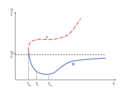
Discontinuous case: Here we discuss the situation in which displays a global minimum appearing exactly at . If is a monotonically increasing function of temperature on the entire big black-hole branch, reaching its maximum value as from below, then clearly it will reach a minimum value (on the big black-hole branch) at , where the big black hole solution ceases to be thermodynamically favored. To work out the behavior of in the range one would then need to switch to the thermal gas solution. Calculating directly in this regime is technically very challenging. However, as outlined in the introduction, there are qualitative field theory arguments which tell us that should start increasing again below , as the temperature continues to drop. Thus, we conclude that in this case corresponds to a global minimum for . This behavior is shown schematically in Figure 6, from which it is also clear that the derivative of is discontinuous at .
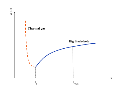
Figure 6: A cartoon of the behavior of in the big black-hole phase (to the right of ) and in the thermal gas phase (for ) for the case where the big black-hole phase is monotonically increasing above . We denote by the temperature above which the correction to is no longer perturbative, and our approximation breaks down. 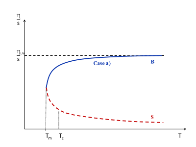
(a)
(b)
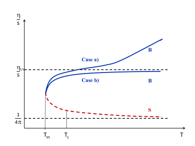
Figure 7: (a) A cartoon of the case when (44) is satisfied, for the type a) potential. (b) A cartoon of the case when (45) is satisfied, for the type a) and type b) potentials labeled respectively by “case a” and “case b.” In both figures denotes the temperature where the small (S) and the big (B) black-hole branches meet and denotes the temperature of the confinement-deconfinement transition. The high temperature value of the viscosity to entropy ratio is denoted by . Graphically it is clear that, in order for this to happen, on the big black-hole branch must approach its high- value from below, and furthermore its derivative on this branch must approach at , where the big and the small black-hole branches meet. Given our assumption that is a monotonic function of on the small black-hole branch, in order to satisfy the second criterion it suffices that decreases as gets larger (in the extreme limit) on the small black-hole branch. By examining (35) and (36) we see that this requires272727Note that we need the derivative of to be positive definite in the asymptotic high- region (on the big black-hole branch). Since is negative definite on the big black-hole branch, we see from (36) that this requires . either of the following two cases:
(44) (45) We plot these two cases schematically in Figure 7(a) and 7(b). Figure 7(a) shows the behavior of on the big (B) and small (S) black-hole branches for a potential whose UV asymptotics are described by case a). In Figure 7(b) on the other hand we include both cases a) and b).
(a)
(b)
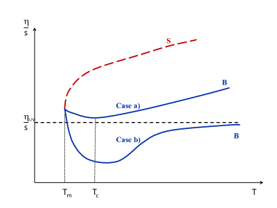
Figure 8: (a) A cartoon of the case when (46) is satisfied. (b) A cartoon of the case when (47) is satisfied. denotes the high- value of , denotes the minimum temperature where the small (S) and the big (B) black-hole branches meet and denotes the temperature of the confinement-deconfinement transition. In Figure (b) we plot both the type a) and type b) potentials labelled by “case a” and “case b” respectively. -
2.
Continuous case: Here the curve has a global minimum on the big black-hole branch at some temperature satisfying . Note that at that point, and all of its derivatives are continuous. For this to happen, clearly must increase as the temperature is raised above , approaching its high-T value from below. More importantly, must also increase below , as the temperature gets closer and closer to . The latter condition translates into the requirement that the derivative on the big black hole branch obeys at . Finally, it suffices that tends upwards on the small black-hole branch282828Recall that we are assuming that is monotonic there., in the limit. Investigation of (35) and (36) reveals that one needs
(46) (47) We provide schematic drawings of these two cases in Figure 8(a) and 8(b). Note also that (46) corresponds to the case plotted in Figure 5(a). Of course one should also incorporate the fact that, in confining theories, the thermodynamically preferred background changes below . Thus, in order to be able to observe a global minimum located at some temperature , one should ensure that , as shown in Figure 8(a).
The four cases depicted in Figures 7(a), 7(b), 8(a) and 8(b) cover most of the physically interesting situations. Qualitatively distinct behavior (for example a maximum rather than a minimum) for arises in the other ranges of and , but we will not discuss it here. Finally, we should note that allowing for a more general scalar coupling to the higher derivative term (i.e. of the racetrack-type) would modify – and potentially significantly complicate – the analysis of the existence of a global minimum. We will not attempt this here.
III.3.1 The Thermal Gas Phase
We would like to close this section by discussing briefly the main difficulties involved with calculating on the thermal gas background which describes temperatures below the deconfinement transition. We emphasize again that in our analysis we did not explicitly compute below , but rather used knowledge of its behavior in the hadronic phase. The main difficulties involved with a direct computation for stem mostly from the need to consider corrections.
To see why this is so, note that the thermal gas solution has no horizon, hence the contribution to the entropy that would come from evaluating the action on the classical saddle292929Note the identification in front of the action. Thus, whenever the on-shell action on a classical saddle is non-vanishing, automatically all of the thermal functions are proportional to . vanishes. However, the finite temperature in the background generates thermal fluctuations of the graviton gas. Thus, the entropy in this case should be calculated by computing the determinant of fluctuations around the classical thermal gas saddle, and as such it is suppressed with respect to the black-hole contribution. As a result, the entropy of the thermal gas is .
Now, let’s move on to the calculation of on the thermal gas background, which can be done by considering fluctuations of the transverse traceless gravitons – in particular, can be related to the flux of transverse gravitons through the horizon, which is proportional to . On the other hand, the small black-hole background asymptotes to the (Lorentzian) thermal gas in the limit of vanishing horizon radius. This tells us that the leading contribution to also vanishes, in the same way in which the contribution to the entropy of the thermal gas vanished. In order to find the finite contribution one has to consider Witten diagrams with quantum loops, which lead to . Thus, although in the thermal gas is of the same order as that for any black-hole background, in order to calculate it one needs to compute the contributions to both and . Such a calculation would involve computing one-loop diagrams in supergravity. This would naively require knowing the spectrum of all supergravity fields which could run in the loops303030Note, however, that one-loop contributions to hydrodynamic long-time tails do not require a detailed understanding of the spectrum of supergravity fields CaronHuot:2009iq . Perhaps a similar simplification occurs for one-loop contributions to . and as such, knowing a genuine string theory embedding of any particular model. This one-loop calculation appears to be a difficult task and we don’t attempt it here.
IV Discussion
Before summarizing our results for the temperature dependence of the shear viscosity in holographic models, we would first like to discuss several properties of in the QCD plasma. Although the viscosity to entropy ratio in the QGP phase is expected to be very small and roughly
comparable to , its precise value is still largely uncertain.
The collective flow observed at RHIC and LHC is analyzed by performing a Fourier decomposition of
the particles’ angular distribution, whose Fourier coefficients are sensitive to transverse momentum .
Restrictions on the possible range of are then extracted from the data either by
comparing the momentum-dependent elliptic flow coefficient with results obtained from viscous
hydrodynamical calculations313131More precisely, one needs a ‘hybrid’ code which combines viscous hydrodynamics of the QGP phase
with a realistic model of the late hadronic stage (see e.g. Heinz:2011kt ).,
or by fitting the centrality dependence of the average integrated elliptic flow.
Both approaches yield bounds on which are somewhat close to the universal value,
with the analysis of Song:2010mg giving .
Uncertainties of
A number of challenges, both theoretical and experimental, have to be overcome in order to determine more precisely.
Uncertainties on the experimental side come from non-flow correlations introduced, for example, by jets and resonance decays. On the theoretical side, uncertainties are due to various assumptions on the choice of initial conditions, initial state
pressure gradients and event-by-event fluctuations.
As an example, it was realized only recently that the assumption that higher order harmonics
were negligible was a poor one – the shape of the fireball can fluctuate from one event to the next, even at a fixed impact parameter.
The resulting irregular pressure gradients are not symmetric with respect to the reaction plane,
and can in fact induce higher harmonic flow patterns.
The elliptic flow direction and magnitude can also fluctuate event-by-event.
Interestingly, the measurement of higher harmonics can play an important role in reducing the degeneracy between the shear viscosity and
initial conditions, and appears to give tighter limits on .
In fact, a combined analysis Qiu:2011hf of elliptic and triangular flow coefficients ( and , respectively)
in Pb Pb collisions at LHC was shown to favor a small shear viscosity , disfavoring the considerably larger
value of (we refer the reader to Muller:2012zq for a more detailed discussion of these issues).
Although none of the models currently used describes perfectly all experimental flow data,
the expectation is that – with the new high precision data coming from LHC – it will be possible
to cut down on such uncertainties and arrive at a precision measurement of the transport properties of the QGP.
The temperature dependence of
Another important issue for disentangling the physics of the QGP is that of the possible temperature dependence of ,
which is the main focus of our analysis.
Although most hydrodynamical simulations of the QGP assume a constant value for ,
a number of studies – mostly qualitative in nature –
have begun to examine the possible relevance of temperature in LHC and RHIC heavy ion collisions
Niemi:2011ix ; Nagle:2011uz ; Shen:2011kn ; Bluhm:2010qf .
First results for the shear and bulk viscosity obtained via lattice QCD simulations
were put forth in Nakamura:2004sy ; Meyer:2007ic , where it was shown that
remains close to its universal value for a range of temperatures not far above .
On the other hand, kinetic theory results for QCD at weak coupling Arnold:2000dr ; Arnold:2003zc
imply , for the QCD running coupling constant in the range .
Elliptic flow values at LHC energies may be sensitive to the temperature behavior of
in the QGP phase, although insensitive to it in the hadronic phase Niemi:2011ix .
Moreover, it was argued in Csernai:2006zz that should have a minimum at (or near) the QCD phase transition.
This is expected because increases with decreasing temperature in the hadronic phase Gavin:1985ph ; Prakash:1993bt , while asymptotic
freedom dictates that it increases with temperature in the deconfined phase – thus leading to at least one minima somewhere in the intermediate region.
An interesting study of shear and bulk viscosities for a finite temperature, pure gluon plasma was performed in Bluhm:2010qf ,
where the authors used a phenomenological, quasi-particle model based on an effective kinetic theory description.
At large temperatures, the results of Bluhm:2010qf reproduce parametrically the transport behavior
observed in perturbative QCD calculations.
As the non-perturbative regime is approached, their analysis is in agreement with lattice QCD results,
with a decrease of with temperature and a minimum at .
Independently of the assumptions behind particular choices of model and simulation schemes, it is clear
that a more systematic understanding of the temperature dependence of
is an important ingredient
towards a better descriptions of the dynamics of the QGP.
IV.1 Summary of Results
The aim of this paper was to initiate a systematic study of the temperature dependence of the shear viscosity in the strongly coupled QGP (and gauge theory plasma more generally), in the framework of the holographic gauge/gravity duality. We were largely motivated by the potential sensitivity of elliptic flow measurements to thermal variations of , but were also interested in gaining further insight into the geometric interpretation of a non-trivial temperature flow for the shear viscosity. We restricted our attention to theories of gravity coupled to a scalar field in the presence of higher derivative corrections,
| (48) |
under the assumption that the coupling is perturbatively small323232From now on we will set the AdS length scale equal to one.. Higher order curvature corrections are well-known to push away from its universal value. Moreover, once they are coupled to a non-trivial scalar field profile, they lead generically to a temperature flow for , as already seen in Buchel:2010wf and emphasized in Cremonini:2011ej .
The correction to – which is parametrized entirely in terms of horizon data – can be expressed in terms of the potential and the horizon value of the scalar field, and for (48) takes the relatively simple form (see Section II for details of the derivation)
| (49) |
Note that thanks to this expression, determining the presence of local minima for is entirely straightforward. In particular, extrema are found by minimizing (49) with respect to333333Assuming that is finite. , and therefore correspond to the zeros of the relation (42). We emphasize that such a condition is rather generic, given the broad assumptions behind (49) – essentially the requirement of AdS asymptotics.
Armed with the general expression (49), we have analyzed a number of holographic setups. For the majority of our analysis, we have restricted our attention to the special case of , for which the viscosity to entropy ratio reduces to
| (50) |
In this class of theories, the (horizon) quantity tracks the temperature of the system. As a result, the behavior of as a function of temperature is controlled by the scalar field coupling to the curvature corrections – parametrized here by and – as well as by the specific functional form of the potential.
As a simple consistency check of our result, we note that for the case of a non-dynamical scalar our expression (50) reduces to a constant and reproduces the standard result for an AdS black-brane in pure gravity with curvature-squared terms. On the other hand, an analytically tractable example which gives rise to non-trivial temperature dependence is that of a single exponential potential, . Black-brane solutions in this system have a temperature of the form . With this choice of potential, our expression (50) implies a monotonic temperature flow for , whose precise structure is shown in (30) and is dictated by the range and signs of and . Interestingly, when the viscosity to entropy ratio takes on a constant value again, with no temperature dependence. In particular, for the specific choice the model can be obtained via a dimensional reduction of a six-dimensional theory of pure gravity with a negative cosmological constant, in the presence of corrections. As expected, our correction to in this case reduces to that for a pure black brane, providing a rather non-trivial check of our result (50). The absence of temperature dependence in this case is then a simple consequence of the fact that the five-dimensional theory inherits the scale invariance of the parent six-dimensional one (see also the discussion in Blaise ).
The behavior of becomes more interesting – and more relevant to the physics of the QGP – for theories which undergo a confinement–deconfinement transition at some critical temperature . In our analysis we have worked mostly with potentials constructed ‘phenomenologically’ by requiring their IR and UV asymptotics to match with expectations from QCD, as in the case of the Improved Holographic QCD (ihQCD) model discussed in Section III.2. However, we emphasize that a number of our results hold more broadly, and can be easily generalized. Plots of the temperature dependence of in the ihQCD model for fiducial values of are shown in Figure 5. On the left, we note the presence of a small minimum slightly above , above which approaches . The behavior for was not computed directly, but rather extrapolated using the fact that is expected to increase in the hadronic phase, as the temperature is lowered. The figure on the right, on the other hand, exhibits a minimum exactly at , with growing indefinitely as the temperature is raised. A cartoon of the same type of behavior – expected to describe more general settings – is shown in Figure 6.
For theories which confine quarks at zero temperature, the thermodynamic structure of the corresponding finite-temperature theory plays an interesting role in determining the behavior of , and enables one to make generic qualitative statements about its temperature flow. In this class of models, the geometry which is favored thermodynamically for is that of a big black hole, while below the dominant phase corresponds to a thermal gas. However, a third solution appears for (with ), which describes a small black-hole solution. For the ihQCD model, the existence of the two black-hole branches can be seen in Figure 4, with the minimum separating the big black hole (on the left) from the small one (on the right). Although the small black-hole is never thermodynamically favored – and is therefore not of any direct physical relevance – it can still be useful for probing in the physically relevant regime . In fact, the coexistence of the small and big black-hole solutions for implies that is double-valued there, and that its derivative diverges at the point where the two branches meet. These features can be seen for example in Figure 7(a). By examining the rough dependence of on temperature on the two branches and the sign of as is approached, one can then reconstruct whether exhibits a minimum in the range.
Following this strategy, in Section IIIC we have derived a set of geometric conditions for the existence of a global minimum for in this class of models343434Under the (mild) assumption that is monotonic on the small black-hole branch.. We have chosen to work with dilatonic potentials which have confining IR asymptotics and exhibit two distinct behaviors in the UV, both consistent with AdS asymptotics – the type a) and type b) potentials corresponding, respectively, to a massless and massive scalar. The requirement – from asymptotic freedom – that approaches its high-T value from below fixes the signs and ranges of the higher derivative couplings and . Combined with the requirement that the zero-temperature theory is confining, it guarantees the existence of a global minimum for at or above the critical temperature, in a certain portion of the phase space. Furthermore, whether the (global) minimum is located exactly at or above it can be determined by looking at the sign of the divergence of at , the point where the big and small black hole branches meet.
In Section IIIC we have provided a geometric classification of these two cases, which we emphasize are physically distinct. The parameter space of the ‘discontinuous’ case, describing a global minimum exactly at , is summarized in (44) and (45), and shown schematically in Figure 7. The ‘continuous’ case, with a global minimum at some temperature , is described instead in (46) and (47), and shown in Figure 8. We note that both cases have (for the precise range of we refer the reader to Section IIIC). The two types of UV asymptotics, cases a) and b), are also shown in the figures. The high-temperature behavior of , and in particular whether it approaches a constant value or increases indefinitely with temperature, is determined by the values and ranges of the , parameters. Another generic result of our analysis is that when the confinement-deconfinement phase transition is second (or higher) order the derivative diverges or vanishes at , depending on the value of the parameter , while remains finite and approaches its universal value353535This result is valid as long as the perturbative approximation can be trusted. See section IIIC for details..
One should note, however, that the holographic demonstration of the existence of a global minimum in confining backgrounds is incomplete. In particular, it is desirable to find an independent holographic reason for the requirement that should be positive, needed for the presence of the global minimum in the continuous/discontinous cases discussed above. In fact, although we always insisted on keeping the correction to perturbatively small (by appropriately turning down ), we relied on the fact that diverges near . Thus, one may worry that any conclusion drawn from using in a regime where it is very large might not be valid. While this is a fair concern, we should note that it is which diverges, with remaining finite (and small). For completeness, it would also be desirable to perform the analogous calculation in the hadronic phase (), and derive holographically the monotonically decreasing behavior of expected from field theory. Finally, we should caution the reader that a more generic higher derivative scalar coupling would give rise to a more complicated structure for (i.e. imagine allowing for racetrack-type terms) and might invalidate some of our arguments for the presence of a global minimum. Clearly, our analysis would have to be re-evaluated in such situations. Regardless, we would like to emphasize that – for a certain class of potentials, and for simple higher derivative couplings of the form – we have translated the issue of the existence of a minimum for into a geometric one, and identified the holographic conditions which would guarantee its presence, complementing the field-theoretic arguments of Kovtun:2011np .
In order for our analysis to be of more direct relevance to studies of the QGP, it is crucial to find ways to place restrictions on the allowed ranges of the couplings and , whether with theory or experiment. This would cut down on the large phase space for the temperature behavior of , and eliminate some of the model dependence inherent in holographic setups of this type – in particular when higher derivative terms are present. At the moment, however, this is very challenging. In the future, it might be feasible to constrain models by examining the effects of higher derivative corrections on the remaining transport coefficients (including those of second order hydrodynamics), and then simultaneously fitting to the available data. While this should be possible in principle, at the moment it presents a serious challenge – the bulk viscosity flows with temperature already without the need for higher derivative terms, and very little is currently known from holography about second order transport coefficients in the presence of higher derivative corrections. On the other hand, it may be possible to restrict the values of the parameters with more phenomenological considerations. As an example, at least in principle we can fit the UV behavior in the type a) potentials we discussed to that predicted by perturbative QCD, which would fix the values of both couplings and . However, we should keep in mind that our analysis is not valid to arbitrarily high temperatures (it breaks down when the higher derivative interactions are no longer perturbative), and therefore any direct comparison with UV physics should be taken with a grain of salt. We leave these questions open for future work.
Acknowledgments
We thank Allan Adams, Peter Arnold, Nabamita Banerjee, Alex Buchel, Anatoly Dymarsky, Suvankar Dutta, Blaise Gouteraux, Elias Kiritsis, Jamie Nagle, Paul Romatschke, Dam Thanh Son, Andrei Starinets, Amos Yarom and Urs Wiedemann for interesting discussions. S.C. is grateful to the Newton Institute for hospitality during the Mathematics and Applications of Branes in String and M-theory workshop while this work was underway. The work of S.C. has been supported by the Cambridge-Mitchell Collaboration in Theoretical Cosmology, and the Mitchell Family Foundation. U.G. is grateful to the University of Crete, the organizers of the Cosmology and Complexity 2012 workshop in Hydra, Greece, and the IMBM (Istanbul Center for Mathematical Sciences) where parts of this work have been completed. The work of P.S. has been supported by the U.S. Department of Energy under Grant No. DE-FG02-97ER41027. This research was supported in part by the National Science Foundation under Grant No. PHY05-51164.
Appendix A The Method of Phase Variables
For the study of dilatonic black hole solutions, it turns out to be particularly convenient to adopt the phase variables method developed in LongThermo , which we briefly review here. With the black brane ansatz
| (51) |
the Einstein and dilaton equations of motion that follow from the action (10) can be put in the following simple form of five first-order equations,
| (52) | |||||
| (53) | |||||
| (54) |
and
| (55) | |||||
| (56) |
where and we have introduced the phase variables
| (57) |
which are invariant under radial coordinate transformations LongThermo . Note that the metric functions and can be expressed in terms of and by integrating directly (57),
| (58) | |||||
| (59) |
where denotes a cut-off surface that plays the role of the regularized UV boundary363636 At the boundary we require , which fixes its dependence on . Moreover, as shown in LongThermo , the physical observables in this system only depend on and and are independent of ..
The advantage of expressing Einstein’s equations in terms of the phase variables should now be apparent – the system has been reduced to a coupled set of first order equations373737In order to solve (55) and (56) one has to specify a single boundary condition for each of the equations. After demanding a regular horizon of the form (60) inspection of the equations (59) and (56) shows that the remaining integration constant is completely fixed, and near one must require (61) , (55) and (56), which greatly simplifies the task of finding analytic solutions. Moreover, all thermodynamic properties of the system are completely determined by knowledge of the two degrees of freedom and as a function of . In fact, in terms of the horizon value of the dilaton, the temperature and the entropy of the black brane are given by
| (62) | |||||
| (63) |
Combining these two expressions we find a simple relation between the phase variable and the scalar potential,
| (64) |
where the proportionality constant is given by
| (65) |
and we have traded Newton’s constant for the Planck mass, . Finally, the temperature can be directly related to the horizon expansion of the blackness function as follows,
| (66) |
These relations greatly facilitate the study of black brane solutions to the model described by (1), as we show in the main text.
Appendix B Chamblin-Reall from Reduction
In this appendix we expand upon the particular case of the Chamblin-Reall black brane. The special case , for which shows no temperature dependence, can be realized as a solution of a dimensionally reduced theory of pure gravity plus a negative cosmological constant in six dimensions. As such this solution can be uplifted to a pure AdS black brane in six-dimensions, thus explaining the temperature independent form for
To see this in more detail, we start from the following Lagrangian density in space-time dimensions,
| (67) |
and perform a circle reduction by decomposing the metric as
| (68) |
where is a scalar383838Note that we have consistently fixed the Kaluza-Klein gauge field to vanish.. The dimensionally reduced theory is then given by
| (69) |
where we fixed to ensure a canonical Einstein term, and omitted higher derivative terms involving and , since they do not affect . Notice that, as expected, we have generated a dilatonic coupling to the Riemann-squared term. However – unlike in (1), where the parameter is free – here the dilatonic coupling is completely fixed in terms of . Thus, we have recovered the model of (1) with the CR potential (20), but only for the special parameter choice .
We can now compute for the dimensionally reduced theory. Restricting to and rescaling the dilaton so that its kinetic term agrees with (1), the lagrangian becomes
| (70) |
Comparing this to our action (1), we see that we have generated a scalar coupling with . The black-brane solution to the two-derivative theory is given in Gouteraux:2011ce ,
| (71) | |||||
| (72) | |||||
| (73) | |||||
| (74) |
and has the following near horizon expansion
| (75) |
Plugging this near horizon expansion into our solution for and taking we arrive at the following result
| (76) |
This is precisely the result expected for an -Schwarzschild black hole in six-dimensions Kats:2007mq . This is expected since, as we have shown, this specific Einstein-dilaton system in 5-dimensions was simply a dimensional reduction of a 6-dimensional theory containing only gravity and a cosmological constant. In fact, the dilaton solution presented may be explicitly uplifted to an -Schwarzschild black hole in six-dimensions Gouteraux:2011ce . While we have focused on a circle reduction from six-dimensions, similar statements can be made for generic n-torus reductions to five-dimensions as in Gubser1 , resulting in Chamblin-Reall theories with
References
- (1) H. Song, S. A. Bass, U. Heinz, T. Hirano and C. Shen, “200 A GeV Au+Au collisions serve a nearly perfect quark-gluon liquid,” Phys. Rev. Lett. 106, 192301 (2011) [arXiv:1011.2783 [nucl-th]].
- (2) D. Teaney, “The Effects of viscosity on spectra, elliptic flow, and HBT radii,” Phys. Rev. C68, 034913 (2003). [nucl-th/0301099].
- (3) M. Luzum, P. Romatschke, “Conformal Relativistic Viscous Hydrodynamics: Applications to RHIC results at s(NN)**(1/2) = 200-GeV,” Phys. Rev. C78, 034915 (2008). [arXiv:0804.4015 [nucl-th]].
- (4) M. Luzum, “Elliptic flow at energies available at the CERN Large Hadron Collider: Comparing heavy-ion data to viscous hydrodynamic predictions,” Phys. Rev. C83, 044911 (2011). [arXiv:1011.5173 [nucl-th]].
- (5) J. L. Nagle, I. G. Bearden, W. A. Zajc, “Quark-Gluon Plasma at RHIC and the LHC: Perfect Fluid too Perfect?,” Submitted to: New J.Phys.. [arXiv:1102.0680 [nucl-th]].
- (6) C. Shen, U. W. Heinz, P. Huovinen, H. Song, “Radial and elliptic flow in Pb+Pb collisions at the Large Hadron Collider from viscous hydrodynamic,” [arXiv:1105.3226 [nucl-th]].
- (7) B. Muller, J. Schukraft and B. Wyslouch, “First Results from Pb+Pb collisions at the LHC,” arXiv:1202.3233 [hep-ex].
- (8) G. Policastro, D. T. Son, A. O. Starinets, “The Shear viscosity of strongly coupled N=4 supersymmetric Yang-Mills plasma,” Phys. Rev. Lett. 87, 081601 (2001). [hep-th/0104066].
- (9) A. Buchel, J. T. Liu, “Universality of the shear viscosity in supergravity,” Phys. Rev. Lett. 93, 090602 (2004). [arXiv:hep-th/0311175 [hep-th]].
- (10) J. Erdmenger, P. Kerner and H. Zeller, “Non-universal shear viscosity from Einstein gravity,” Phys. Lett. B 699, 301 (2011) [arXiv:1011.5912 [hep-th]].
- (11) J. Casalderrey-Solana, H. Liu, D. Mateos, K. Rajagopal, U. A. Wiedemann, “Gauge/String Duality, Hot QCD and Heavy Ion Collisions,” [arXiv:1101.0618 [hep-th]].
- (12) A. Adams, L. D. Carr, T. Schaefer, P. Steinberg and J. E. Thomas, “Strongly Correlated Quantum Fluids: Ultracold Quantum Gases, Quantum Chromodynamic Plasmas, and Holographic Duality,” arXiv:1205.5180 [hep-th].
- (13) A. Sinha and R. C. Myers, “The Viscosity bound in string theory,” Nucl. Phys. A 830, 295C (2009) [arXiv:0907.4798 [hep-th]].
- (14) S. Cremonini, “The Shear Viscosity to Entropy Ratio: A Status Report,” Mod. Phys. Lett. B25, 1867-1888 (2011). [arXiv:1108.0677 [hep-th]].
- (15) N. Banerjee and S. Dutta, “Holographic Hydrodynamics: Models and Methods,” arXiv:1112.5345 [hep-th].
- (16) R. -G. Cai, Z. -Y. Nie and Y. -W. Sun, “Shear Viscosity from Effective Couplings of Gravitons,” Phys. Rev. D 78, 126007 (2008) [arXiv:0811.1665 [hep-th]].
- (17) R. C. Myers, M. F. Paulos, A. Sinha, “Holographic Hydrodynamics with a Chemical Potential,” JHEP 0906, 006 (2009). [arXiv:0903.2834 [hep-th]].
- (18) S. Cremonini, K. Hanaki, J. T. Liu, P. Szepietowski, “Higher derivative effects on eta/s at finite chemical potential,” Phys. Rev. D80, 025002 (2009). [arXiv:0903.3244 [hep-th]].
- (19) R. -G. Cai, Z. -Y. Nie, N. Ohta and Y. -W. Sun, “Shear Viscosity from Gauss-Bonnet Gravity with a Dilaton Coupling,” Phys. Rev. D 79, 066004 (2009) [arXiv:0901.1421 [hep-th]].
- (20) S. Cremonini and P. Szepietowski, “Generating Temperature Flow for eta/s with Higher Derivatives: From Lifshitz to AdS,” JHEP 1202, 038 (2012) [arXiv:1111.5623 [hep-th]].
- (21) A. Buchel, S. Cremonini, “Viscosity Bound and Causality in Superfluid Plasma,” JHEP 1010, 026 (2010). [arXiv:1007.2963 [hep-th]].
- (22) A. Ghodsi and M. Alishahiha, “Non-relativistic D3-brane in the presence of higher derivative corrections,” Phys. Rev. D 80, 026004 (2009) [arXiv:0901.3431 [hep-th]].
- (23) P. Basu and J. -H. Oh, “Analytic Approaches to An-Isotropic Holographic Superfluids,” arXiv:1109.4592 [hep-th].
- (24) J. Erdmenger, P. Kerner and H. Zeller, “Transport in Anisotropic Superfluids: A Holographic Description,” JHEP 1201, 059 (2012) [arXiv:1110.0007 [hep-th]].
- (25) A. Rebhan and D. Steineder, “Violation of the Holographic Viscosity Bound in a Strongly Coupled Anisotropic Plasma,” Phys. Rev. Lett. 108, 021601 (2012) [arXiv:1110.6825 [hep-th]].
- (26) J. -H. Oh, “Running Shear Viscosities in An-Isotropic Holographic Superfluids,” arXiv:1201.5605 [hep-th].
- (27) K. A. Mamo, “Holographic Wilsonian RG Flow of the Shear Viscosity to Entropy Ratio in Strongly Coupled Anisotropic Plasma,” arXiv:1205.1797 [hep-th].
- (28) L. P. Csernai, J. .I. Kapusta and L. D. McLerran, “On the Strongly-Interacting Low-Viscosity Matter Created in Relativistic Nuclear Collisions,” Phys. Rev. Lett. 97, 152303 (2006) [nucl-th/0604032].
- (29) S. Gavin, “Transport Coefficients In Ultrarelativistic Heavy Ion Collisions,” Nucl. Phys. A 435, 826 (1985).
- (30) M. Prakash, M. Prakash, R. Venugopalan and G. Welke, “Nonequilibrium properties of hadronic mixtures,” Phys. Rept. 227, 321 (1993).
- (31) J. Noronha-Hostler, J. Noronha and C. Greiner, “Transport Coefficients of Hadronic Matter near T(c),” Phys. Rev. Lett. 103, 172302 (2009) [arXiv:0811.1571 [nucl-th]].
- (32) P. B. Arnold, G. D. Moore and L. G. Yaffe, “Transport coefficients in high temperature gauge theories. 1. Leading log results,” JHEP 0011, 001 (2000) [hep-ph/0010177].
- (33) P. B. Arnold, G. DMoore and L. G. Yaffe, “Transport coefficients in high temperature gauge theories. 2. Beyond leading log,” JHEP 0305, 051 (2003) [hep-ph/0302165].
- (34) P. J. Linstrom, W. G. Mallard, Eds., NIST Chemistry WebBook, NIST Standard Reference Database Number 69, National Institute of Standards and Technology; http://webbook.nist.gov.
- (35) P. Massignan, G. M. Bruun and H. Smith, “Viscous relaxation and collective oscillations in a trapped Fermi gas near the unitarity limit,” Phys. Rev. A 71, 033607 (2005) [cond-mat/0409660 [cond-mat.stat-mech]].
- (36) M. Mannarelli, C. Manuel and L. Tolos, “Shear viscosity in a superfluid cold Fermi gas at unitarity,” arXiv:1201.4006 [cond-mat.quant-gas].
- (37) H. Song, S. A. Bass, U. Heinz, T. Hirano and C. Shen, “Hadron spectra and elliptic flow for 200 A GeV Au+Au collisions from viscous hydrodynamics coupled to a Boltzmann cascade,” Phys. Rev. C 83, 054910 (2011) [arXiv:1101.4638 [nucl-th]].
- (38) R. A. Lacey, N. N. Ajitanand, J. M. Alexander, P. Chung, W. G. Holzmann, M. Issah, A. Taranenko and P. Danielewicz et al., “Has the QCD Critical Point been Signaled by Observations at RHIC?,” Phys. Rev. Lett. 98, 092301 (2007) [nucl-ex/0609025].
- (39) H. Niemi, G. S. Denicol, P. Huovinen, E. Molnar, D. H. Rischke, “Influence of the shear viscosity of the quark-gluon plasma on elliptic flow in ultrarelativistic heavy-ion collisions,” Phys. Rev. Lett. 106, 212302 (2011). [arXiv:1101.2442 [nucl-th]].
- (40) C. Shen, U. Heinz, “Hydrodynamic flow in heavy-ion collisions with large hadronic viscosity,” Phys. Rev. C83, 044909 (2011). [arXiv:1101.3703 [nucl-th]].
- (41) M. Bluhm, B. Kampfer and K. Redlich, “Bulk and shear viscosities of the gluon plasma in a quasiparticle description,” Phys. Rev. C 84, 025201 (2011) [arXiv:1011.5634 [hep-ph]].
- (42) P. Kovtun, G. D. Moore and P. Romatschke, “The stickiness of sound: An absolute lower limit on viscosity and the breakdown of second order relativistic hydrodynamics,” Phys. Rev. D 84, 025006 (2011) [arXiv:1104.1586 [hep-ph]].
- (43) U. Gursoy and E. Kiritsis, “Exploring improved holographic theories for QCD: Part I,” JHEP 0802, 032 (2008) [arXiv:0707.1324 [hep-th]].
- (44) U. Gursoy, E. Kiritsis and F. Nitti, “Exploring improved holographic theories for QCD: Part II,” JHEP 0802, 019 (2008) [arXiv:0707.1349 [hep-th]].
- (45) A. Buchel, J. T. Liu, A. O. Starinets, “Coupling constant dependence of the shear viscosity in N=4 supersymmetric Yang-Mills theory,” Nucl. Phys. B707, 56-68 (2005). [hep-th/0406264].
- (46) N. Iqbal, H. Liu, “Universality of the hydrodynamic limit in AdS/CFT and the membrane paradigm,” Phys. Rev. D79, 025023 (2009). [arXiv:0809.3808 [hep-th]].
- (47) U. Gursoy, E. Kiritsis, L. Mazzanti and F. Nitti, “Holography and Thermodynamics of 5D Dilaton-gravity,” JHEP 0905 (2009) 033 [arXiv:0812.0792 [hep-th]].
- (48) Y. Kats and P. Petrov, Effect of curvature squared corrections in AdS on the viscosity of the dual gauge theory, JHEP 0901, 044 (2009) [arXiv:0712.0743 [hep-th]].
- (49) M. Brigante, H. Liu, R. C. Myers, S. Shenker and S. Yaida, Phys. Rev. D 77, 126006 (2008) [arXiv:0712.0805 [hep-th]].
- (50) H. A. Chamblin and H. S. Reall, “Dynamic dilatonic domain walls,” Nucl. Phys. B 562 (1999) 133 [hep-th/9903225].
- (51) B. Gouteraux, J. Smolic, M. Smolic, K. Skenderis and M. Taylor, “Holography for Einstein-Maxwell-dilaton theories from generalized dimensional reduction,” JHEP 1201, 089 (2012) [arXiv:1110.2320 [hep-th]].
- (52) T. Wiseman and B. Withers, “Holographic renormalization for coincident Dp-branes,” JHEP 0810, 037 (2008) [arXiv:0807.0755 [hep-th]].
- (53) S. S. Gubser and A. Nellore, “Mimicking the QCD equation of state with a dual black hole,” Phys. Rev. D 78 (2008) 086007 [arXiv:0804.0434 [hep-th]].
- (54) C. Charmousis, B. Gouteraux and E. Kiritsis, “Higher-derivative scalar-vector-tensor theories: black holes, Galileons, singularity cloaking and holography,” arXiv:1206.1499 [hep-th].
- (55) U. Gursoy, E. Kiritsis, L. Mazzanti and F. Nitti, “Deconfinement and Gluon Plasma Dynamics in Improved Holographic QCD,” Phys. Rev. Lett. 101 (2008) 181601 [arXiv:0804.0899 [hep-th]].
-
(56)
J. M. Maldacena,
“Wilson loops in large N field theories,”
Phys. Rev. Lett. 80 (1998) 4859
[hep-th/9803002].
S. -J. Rey and J. -T. Yee, “Macroscopic strings as heavy quarks in large N gauge theory and anti-de Sitter supergravity,” Eur. Phys. J. C 22 (2001) 379 [hep-th/9803001]. - (57) U. Gursoy, E. Kiritsis, L. Mazzanti and F. Nitti, “Improved Holographic Yang-Mills at Finite Temperature: Comparison with Data,” Nucl. Phys. B 820 (2009) 148 [arXiv:0903.2859 [hep-th]].
- (58) M. Caselle, L. Castagnini, A. Feo, F. Gliozzi, U. Gursoy, M. Panero and A. Schafer, “Thermodynamics of SU(N) Yang-Mills theories in 2+1 dimensions II. The Deconfined phase,” arXiv:1111.0580 [hep-th].
- (59) K. Veschgini, E. Megias and H. J. Pirner, “Trouble Finding the Optimal AdS/QCD,” Phys. Lett. B 696, 495 (2011) [arXiv:1009.4639 [hep-th]].
- (60) U. Gursoy, “Continuous Hawking-Page transitions in Einstein-scalar gravity,” JHEP 1101, 086 (2011) [arXiv:1007.0500 [hep-th]].
- (61) S. Caron-Huot and O. Saremi, “Hydrodynamic Long-Time tails From Anti de Sitter Space,” JHEP 1011, 013 (2010) [arXiv:0909.4525 [hep-th]].
- (62) U. W. Heinz, C. Shen and H. Song, “The viscosity of quark-gluon plasma at RHIC and the LHC,” AIP Conf. Proc. 1441, 766 (2012) [arXiv:1108.5323 [nucl-th]].
- (63) Z. Qiu, C. Shen and U. Heinz, “Hydrodynamic elliptic and triangular flow in Pb-Pb collisions at sqrt(s)=2.76ATeV,” Phys. Lett. B 707, 151 (2012) [arXiv:1110.3033 [nucl-th]].
- (64) A. Nakamura and S. Sakai, “Transport coefficients of gluon plasma,” Phys. Rev. Lett. 94, 072305 (2005) [hep-lat/0406009].
- (65) H. B. Meyer, “A Calculation of the shear viscosity in SU(3) gluodynamics,” Phys. Rev. D 76, 101701 (2007) [arXiv:0704.1801 [hep-lat]].
- (66) B. Gouteraux and E. Kiritsis, “Generalized Holographic Quantum Criticality at Finite Density,” JHEP 1112, 036 (2011) [arXiv:1107.2116 [hep-th]].