A one-dimensional Fermi accelerator model with moving wall described by a nonlinear van der Pol oscillator

Abstract

A modification of the one-dimensional Fermi accelerator model is considered in this work. The dynamics of a classical particle of mass $m$, confined to bounce elastically between two rigid walls where one is described by a non-linear van der Pol type oscillator while the other one is fixed, working as a re-injection mechanism of the particle for a next collision, is carefully made by the use of a two-dimensional non-linear mapping. Two cases are considered: (i) the situation where the particle has mass negligible as compared to the mass of the moving wall and does not affect the motion of it; (ii) the case where collisions of the particle does affect the movement of the moving wall. For case (i) the phase space is of mixed type leading us to observe a scaling of the average velocity as a function of the parameter ($\chi$) controlling the non-linearity of the moving wall. For large $\chi$, a diffusion on the velocity is observed leading us to conclude that Fermi acceleration is taking place. On the other hand for case (ii), the motion of the moving wall is affected by collisions with the particle. However due to the properties of the van der Pol oscillation, the moving wall relaxes again to a limit cycle. Such kind of motion absorbs part of the energy of the particle leading to a suppression of the unlimited energy gain as observed in case (i). The phase space shows a set of attractors of different periods whose basin of attraction has a complicate organization.

I Introduction

As firstly proposed by Enrico Fermi Ref1 as an attempt to describe the high energy of cosmic particles interacting with moving magnetic clouds, the Fermi accelerator model consists of a classical particle of mass $m$ (denoting the cosmic particle) confined to bounce between two rigid walls. One is periodically moving in time (making allusions to the moving magnetic clouds) while the other one is fixed (working as a returning mechanism for a next collision with the moving wall). The phase space of the model is defined by the type of the motion of the moving wall. For a smoothly periodic motion, say a sinusoidally function, periodic islands, chaotic seas and a set of invariant KAM curves are all observed coexisting in the phase space. The diffusion in the velocity is limited by the KAM curves and, deceptively, Fermi acceleration (unlimited energy growth) is not observed. On the other hand when the motion of the moving wall is considered of saw-tooth type, the mixed structure of the phase space is not observed anymore and unlimited energy is observed. The interest in Fermi acceleration has then increased and several applications have been observed in different areas of science including astrophysics Ref2 ; Ref3 , plasma physics Ref4 , optics Ref5 ; Ref6 , atomic physics Ref7 and even in time dependent billiard problems Ref8 . The traditional approach to describe Fermi acceleration developing in such type of time dependent system is generally given in terms of a diffusion process which takes place in momentum space. The evolution of the probability density function for the magnitude of particle velocities as a function of the number of collisions is determined by the Fokker-Planck equation and results for the one-dimensional case consider either static wall approximation and moving boundary description Ref9 ; Ref10 ; Ref11 . The phenomenon however seems not to be robust since dissipation is assumed to be a mechanism to suppress Fermi acceleration Ref12 .

In this paper we revisit the one-dimensional Fermi accelerator model however considering the motion of the moving wall given by a van der Pol type and considering two cases: (i) the mass of the particle is negligible as compared to mass of the moving wall; (ii) the collisions of the particle affect the motion of the moving wall, which are restored to a limit cycle after a relaxation time. Our main goal is to understand and describe the influences of a limit cycle type motion of the moving wall to the dynamics of the particle and hence to the properties of the average velocity in the phase space. To the best knowledge of the authors, this is the first time this approach is considered in this model and the results may have applications to different set of models, particularly to the class of time-dependent billiard problems. The model then consists of a classical particle of mass $m$ which suffers collisions with two walls. One is moving in time whose motion is described by a van der Pol equation leading to a limit cycle dynamics while the other one is fixed and works as a returning mechanism of the particle to a next collision with the moving wall. The dynamics is constructed by a two dimensional nonlinear mapping for the variables velocity of the particle and time. For case (i) the dynamics leads to a mixed phase space structure where periodic islands are observed surrounded by chaotic seas and limited by a set of invariant KAM curves. As soon as the parameter $\chi$ controlling the non-linearity of the moving wall raises, the position of the lowest invariant KAM curve raises too leading to an increase in the average velocity of the particle. Scaling arguments are used to describe the behavior of the average velocity as a function of the parameter $\chi$ and a set of critical exponents are obtained. On the other hand for case (ii), the collisions of the particle with the moving wall indeed affect the dynamics of such wall, leading it out/in of the limit cycle. After a relaxation time however, the moving wall reaches the limit cycle again. A set of different periodic attractors is observed in the phase space and the organization of the basin of attraction of each attractor shows to be complicate. A histogram of periodic orbits is also constructed leading us to observe a high incidence of low period orbits as compared to large period.

This paper is organized as follows. In Sec. II we construct the model and describe the equations that give the dynamics of the motion. Section III is devoted to discuss the case of negligible mass of the particle including results of the phase space, characterization of chaotic orbits and scaling of the average velocity. The case where collisions of the particle affect the motion of the moving wall is described in Sec. IV. Conclusions and final remarks are drawn in Sec. V.

II The model and the mapping

In this section we present all the details needed for the construction of the mapping. The model consists of a classical particle of mass $m$ which is confined to bounce between two walls. One of the them is assumed to be fixed at position $x=L$ and collisions are assumed to be elastic. The other one moves in time and the oscillations are described by a van der Pol oscillator whose average position is $x=0$. We describe two situations where: (i) the mass of the particle is sufficiently small as compared to the mass of the moving wall and, (ii) the case where the mass of the particle is not negligible therefore affecting the dynamics of the moving wall.

Indeed, the van der Pol oscillator is a generalization of a harmonic oscillator that contains a nonlinear and dissipative term. Applications of the van der Pol oscillator can be found in many different systems including dusty plasma Ref13 ; Ref14 , coupled oscillators Ref15 ; Ref16 and many others. The differential equation describing the van der Pol oscillator is defined as

$$M\frac{d^{2}x}{dt^{2}}+b(x^{2}-{x_{0}}^{2})\frac{dx}{dt}+kx=F_{0}\sin(\omega_{f}t)~{},$$ (1)

where $M$ is the mass, $b$ denotes the dissipative term and $k$ is the Hook’s constant. The nonlinear term $(x^{2}-{x_{0}}^{2})$ creates a competition between adding and subtracting energy to/from the system. When $|x|<|x_{0}|$ there is a frictional drag force while for $|x|>|x_{0}|$ there is a negative friction. This competition has a balance of energy such that the sum of the added and reduced energy in a cycle is zero, therefore creating a periodic motion which is commonly called in the literature as limit cycle. When $b\approx 0$ there is a sinusoidal motion with a quasi-circular limit cycle of radius $2x_{0}$. With the growth of $b$, the limit cycle changes to a particular form and the time of relaxation of the oscillator becomes shorter. Figure 1 shows a typical phase space obtained from numerical integration of Eq. (1), by using the Gauss-Radau Ref17 integrator, for the parameters $M=k=x_{0}=1$, $F_{0}=0$ and: (a) $b=0.05$; (b) $b=0.5$ and; (c) $b=10$.

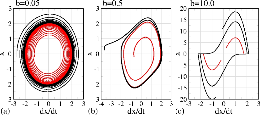
Figure 1: (Color online) Phase space plot for a van der Pol oscillator considering the parameters $M=k=x_{0}=1$ and: (a) $b=0.05$; (b) $b=0.5$ and; (c) $b=10$.

To describe the model itself, we have to define a set of dimensionless and therefore more convenient variables. Defining $y=x/L$ and $\tau=t\omega_{0}$ the equation is rewritten as

$$\frac{d^{2}y}{d{\tau}^{2}}+\chi({y}^{2}-{y_{0}}^{2})\frac{dy}{d\tau}+y=0.$$ (2)

where $\chi=b/(M\omega_{0}L)$ and $y_{0}=x_{0}/L$ and $F_{0}$ was set as null. With this new variables, the distance between the average position of the moving wall and fixed wall becomes dimensionless and equals $1$.

In our description and to determine the law that describes the collisions, we assumed that the momentum and energy are conserved at the instant of each collision. With this approach, the velocities of the particle and the moving wall after the $(n+1)^{th}$ collision are

$$v^{p}_{n+1}=\frac{\mu-1}{1+\mu}(v^{p}_{n}-v^{w}_{n})+v^{w}_{n},$$

$$v^{w}_{n+1}=\frac{2\mu}{1+\mu}(v^{p}_{n}-v^{w}_{n})+v^{w}_{n}.$$ (3)

where the upper index $p$ and $w$ stand for the particle and moving wall respectively. Here $\mu=m/M$ denotes the ratio of mass of the particle and the mass of the moving wall. Therefore the particle and the moving wall change energy and momentum upon collision. In the general case, after the collision of the particle with the moving wall and, due to the change of energy, the velocity of the moving wall changes therefore bringing the moving wall out of the limit cycle. However and depending on the control parameters, the limit cycle is approached again asymptotically. Therefore we have to consider two separate cases: (i) $\mu=0$ and; (ii) $\mu\neq 0$. For case (i), i.e., when the mass of the particle is sufficiently small as compared to the mass of the moving wall $m\ll M$ leading to the limit of $\mu=0$. For this case we assumed that either energy and velocity of the moving wall are not changed after the collision, therefore $v^{w}_{n+1}=v^{w}_{n}$. For case (ii) where $\mu>0$, the collisions of the particle with the moving wall indeed affect the motion of the moving wall bringing it in or out of the limit cycle. It however relaxes again to the limit cycle as time evolves. We therefore consider the two cases in separate sections.

III The case of $\mu=0$

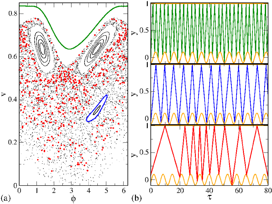
Figure 2: (Color online) (a) Phase space for mapping (4) for the parameters $y_{0}=0.05$ and $\chi=0$. (b) Show the three types of behavior observed in (a): green for KAM curves, blue for periodic islands and red for chaotic dynamics.

In this section we discuss the case of $\mu=0$. It implies that the velocity of the moving wall is not affected by the change of energy with the particle i.e., $v^{w}_{n+1}=v^{w}_{n}$. Moreover, once relaxed to the limit cycle, the moving wall stays in such a regime forever. For such a dynamical regime, we can also calculate a period of oscillation $T$. The dynamics is then described by a two-dimensional mapping for the variables velocity of the particle and phase of the moving wall

$$\phi_{n+1} = [\phi_{n}+\Delta t_{n+1}]~{}mod~{}T,$$

$$v_{n+1} = 2v_{w}(\phi_{n+1})\pm v_{n},$$ (4)

where the $+$ sign of second term stands for successive collisions while $-$ denotes non successive collisions. A successive collision is defined as a collision that the particle has with the moving wall without leaving the collision zone, i.e., without been reflected backwards by the fixed wall. Here $\phi_{n}$ is the phase of the moving wall while $v_{n}$ is the velocity of the particle and the index $n$ denotes the instant of the $n^{th}$ collision with the moving wall. The term $v_{w}(\phi)$ represents the velocity of the moving wall that is obtained numerically from the integration of the van der Pol oscillator (Eq. 2). It indeed has two relevant control parameters namely, $y_{0}$ and $\chi$. The parameter $y_{0}$ controls the amplitude of the limit cycle and $\chi$ controls the amplitude of nonlinear dissipative term. The term $\Delta t_{n+1}$ is solved numerically from the equation

$$\Delta t_{n+1}=\frac{2-x_{w}(\phi_{n})-x_{w}(\phi_{n+1})}{v_{n}},$$

for successive collisions and

$$\Delta t_{n+1}=\frac{x_{w}(\phi_{n+1})-x_{w}(\phi_{n})}{v_{n}},$$

for non successive collisions. For the case of $\mu=0$, the mapping preserves the following measure in the phase space $du={(v-v_{w}(\phi))d\phi dv}$.

The phase space for the case of $\mu=0$ is mixed and periodic islands, KAM curves and a chaotic sea are observed, as shown in Fig. 2 (a). The colors in the three plots of Fig. 2(b), showing trajectory of the particle as a function of time, denote the three types of behavior observed in (a): (i) green for KAM curves; (ii) blue for periodic islands and; (iii) red for chaotic dynamics. Indeed the dynamics along a KAM curve is quasi-regular leading to a small variance of the velocity of the particle while all phases are in principle allowed leading to a seemingly closed curve as shown in Fig. 2(a). For periodic islands, i.e., the case of Fig. 2(b) the orbit has a regular motion and visits only a finite portion of the space including a specific region in phase. The last case (iii) of chaotic motion shows an apparently erratic trajectory in the phase space.

Let us now discuss some properties of the phase space. Indeed the parameter $\chi$ controls the shape of the limit cycle. For $\chi\approx 0$ the present model recovers the results of the Fermi-Ulam model (FUM) Ref18 . In the FUM, the moving wall is described by a sinusoidally function and, as expected, the phase space is mixed. A plot of the phase space for the parameters $y_{0}=0.05$ and $\chi=0$ is shown in Fig. 2(a). With the increase of $\chi$, the shape of the limit cycle changes. Figure 3 shows

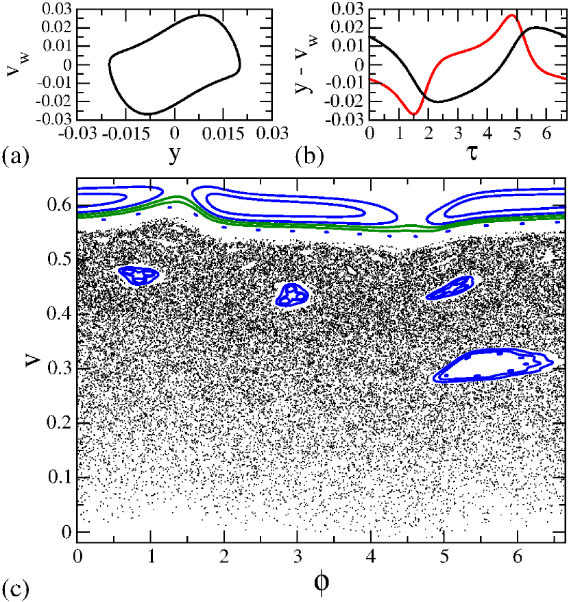
Figure 3: (Color online) (a) Plot of the phase space for moving wall, $v_{w}~{}versus~{}y$; (b) plot of $v_{w}~{}versus~{}\tau$ (red line) and $y~{}versus~{}\tau$ (black line); (c) phase space for the mapping (4) $v~{}versus~{}\phi$. The control parameters used were $\chi=10^{4}$ and $y_{0}=0.01$.

the plots of: (a) the phase space for moving wall, $v_{w}~{}versus~{}y$; (b) plot of $v_{w}~{}versus~{}\tau$ (red line) and $y~{}versus~{}\tau$ (black line) while (c) shows a plot of phase space for the mapping (4) $v~{}versus~{}\phi$. The control parameters used in all plots were $\chi=10^{4}$ and $y_{0}=0.01$.

For a large value of the parameter $\chi$, for example $\chi=10^{5}$, the phase space generated from mapping (4) has, at first sight, a strange form where a not conventional structure is clearer shown. Figure 4

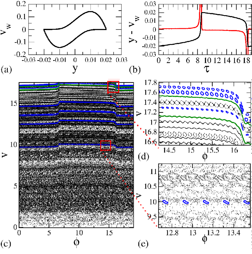
Figure 4: (Color online) (a) Plot of the phase space for moving wall, $v_{w}~{}versus~{}y$; (b) plot of $v_{w}~{}versus~{}\tau$ (red line) and $y~{}versus~{}\tau$ (black line); (c) phase space for the mapping (4) $v~{}versus~{}\phi$. The control parameters used were $\chi=10^{5}$ and $y_{0}=0.01$.

shows the corresponding plots of: (a) the phase space for moving wall, $v_{w}~{}versus~{}y$; (b) plot of $v_{w}~{}versus~{}\tau$ (red line) and $y~{}versus~{}\tau$ (black line) while (c) shows a plot of phase space for the mapping (4) $v~{}versus~{}\phi$. Indeed a zoom-in shown in (d) and (e) exhibit in a minor scale, the structures expected to be observed in mixed phase space. In the reference video1 a video is shown to demonstrate the change of parameter $\chi$ cause in phase space of the particle.

The modifications caused in the dynamics of the particle due to the increase of the parameter $\chi$ may affect some observables in the phase space. Particularly the position of the lowest KAM curve is raised by a raise in $\chi$, leading the particle to acquires more energy from the moving wall. In what follows, our investigation is as function of the parameter $\chi$. To do so, we chose to describe the behavior of the average velocity of the particle along the chaotic orbits as well as the behavior of the positive Lyapunov exponent.

Let us start with the average velocity. To do so, we consider the evolution of the average velocity of the particle as a function of the number of collisions $n$ as well as the parameters $y_{0}$ and $\chi$. The average velocity is obtained as

$$<v(n)>=\frac{1}{K}\sum_{i=1}^{K}v_{i}(n),$$ (5)

where $K$ denotes the total number of initial conditions (ensemble of different particles) and $v_{i}(n)$ is the average velocity obtained along the orbit for a single initial condition. It is defined as

$$v_{i}(n)=\frac{1}{n}\sum_{j=1}^{n}v(j)$$ (6)

where the index $i$ corresponds to one orbit of the ensemble $K$. This kind of ensemble average is widely used in many different dynamical systems Ref18 ; Ref19 ; Ref20 ; Ref21 ; Ref22 . Several tests were made and shown that a results with low fluctuation is obtained with an ensemble of initial condition $K$ of the order $500$ to $1000$. The simulations involved in the calculation of $<v(n)>$ are extremely time consuming especially due to the numerical solution of Eq. 2. As an attempt to speed up the simulations, we introduced a new method to calculate the average velocity. Indeed it can be used because the mapping preserves a measure in the phase space and, due to Poincaré recurrence theorem, the particle may returns to close to a neighboring region to where it started as one wants.

Suppose a time series $v(n)$ is given, where $n=1,2...N$. We define $v_{m}$ as a sup value of velocity for region of low energy in the phase space that belongs to the chaotic sea. Indeed $v_{m}$ should be larger than the velocity of the moving wall and at the same time should be smaller as compared to first KAM curve. Then we construct a vector $k(i)$ where $k$ is a series from each $n$ for those velocities where the condition $v(n)<v_{m}$ is observed such that $i$ is an index that represents the times this will occur. Thus we define the transformations

$$v_{i}(n)=\frac{1}{n}\sum_{j=1}^{n-1}v(j-k(i)),$$ (7)

and

$$<v>(n)=\lim_{N\rightarrow\infty}\frac{1}{K^{\prime}}\sum_{i=1}^{K^{\prime}}v_{i}(n),$$ (8)

where $K^{\prime}=dim(k)$, and $dim$ denotes the dimension of vector $k$. Using this procedure, the evolution of a single orbit for a long time is enough to obtain the average properties and therefore to speed up the simulations as compared to the normal method of evolving a long ensemble of different initial conditions. To have an idea of the accuracy of the proposed method, Fig. 5

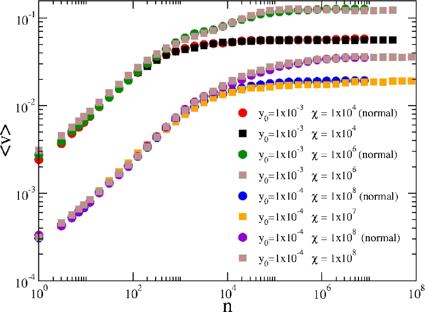
Figure 5: (Color online) Plot of $<v>~{}versus~{}n$ for different control parameters and initial conditions, as labeled in the figure. Bullets denote the traditional (normal) method of evolving an ensemble of initial conditions and squared correspond to the proposed method.

shows a plot of $<v>~{}versus~{}n$ for different control parameters and initial conditions, as labeled in the figure. Bullets correspond to the traditional (normal) method of evolving an ensemble of initial conditions Ref18 while squares denote the proposed method. We see that curve generated by the two methods remarkably overlap each other confirming the procedure can be used. Of course some cautions were taken as for example when the particle is trapped in a sticky region. In this case the problem is fixed by just increasing the number of collisions or by a change the initial condition.

Established the procedure to obtain the average velocity, let us now discuss some properties as a function of the control parameters. Indeed, starting with an initial condition with low velocity, the average velocity $<v>$ grows for small values of $n$ and, after passing by a crossover regime, it becomes constant for large enough $n$. The changeover from growth to the regime marked by a constant plateau defines a final average velocity $<v>_{f}$. Figure 6

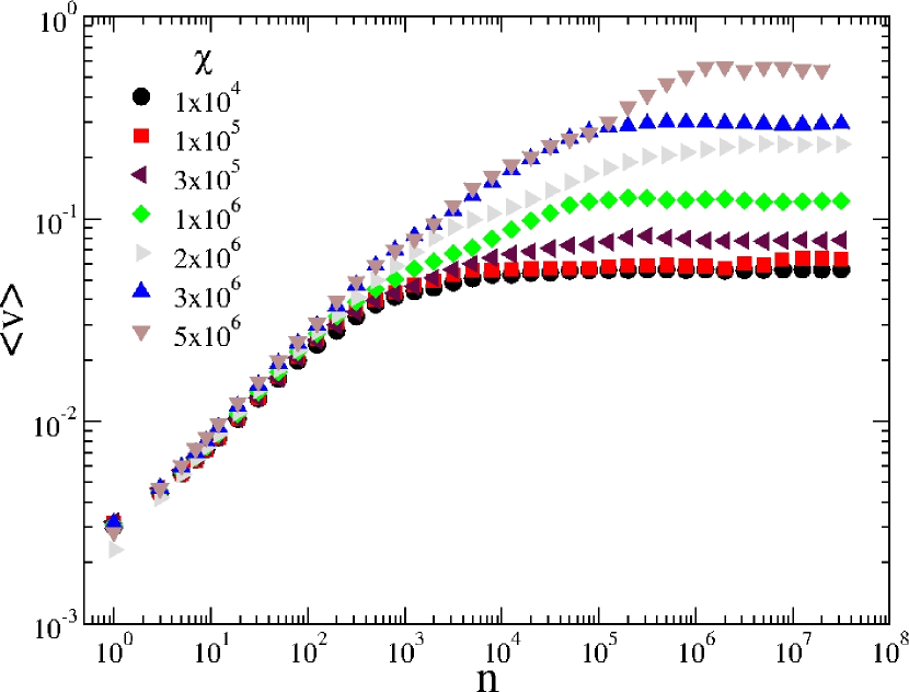
Figure 6: (Color online) Plot of the average velocity as a function of $n$ for the parameter $y_{0}=0.001$ and different values of $\chi$, as labeled in the figure.

shows different plots of $<v>~{}versus~{}n$ for the parameter $y_{0}=0.001$ and different values of $\chi$, as labeled in the figure. For $\chi\approx 0$, the results obtained recover those already known for the traditional FUM Ref18 . As shown in Fig. 6, a change in $\chi$ leads the asymptotic dynamics for large $n$ to reach different saturation of the velocity. It is expected that a similar behavior is to be observed as the parameter $y_{0}$ varies and it indeed happens. A plot of the final average velocity $<v>_{f}$ as a function of the parameter $y_{0}$ is shown in Fig. 7(a).

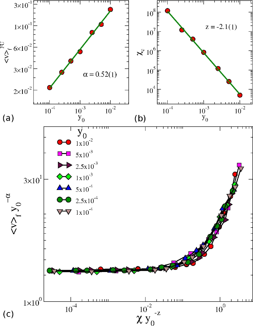
Figure 7: (Color online) (a) Plot of $<v>_{f}^{FU}~{}versus~{}y_{0}$. A fitting furnishes an exponent $\alpha=0.52(2)$; (b) Plot of $\chi_{c}~{}versus~{}y_{0}$. A numerical fit gives an exponent $z=-2.1(2)$; (c) Overlap of different curves of $<v>$ onto a single plot, after a suitable rescale of the axis, for different control parameters, as labeled in the figure.

The behavior of the final average velocity as a function of $\chi$ is shown in Fig. 8

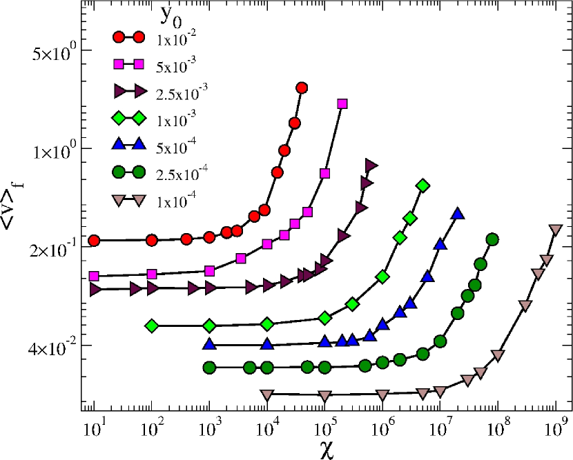
Figure 8: (Color online) Plot of the final average velocity as a function of $\chi$ for different values of $y_{0}$, as labeled in the figure.

for different values of $y_{0}$, as labeled in the figure. We see from this figure that the final average velocity stays in a plateau for a large range of $\chi$ and that it depends on $y_{0}$. After a critical parameter $\chi_{c}$ is reached, the average velocity starts to increase with a power law. Based on the behavior observed in Fig. 8, we propose the following:

1. For $\chi\ll{\chi_{c}}$, the average velocity $<v>_{f}$ behaves as

   $$<v>_{f}(\chi)\propto y_{0}^{\alpha}~{},$$ (9)

   where $\alpha$ is a critical exponent;

2. For $\chi\gg{\chi_{c}}$, the average velocity is written as

   $$<v>_{f}(\chi)\propto\chi^{\beta}~{},$$ (10)

   where $\beta$ is also a critical exponent;

3. Finally, the crossover $\chi_{c}$ that marks the change from the plateau to the regime of growth is given by

   $$\chi_{c}\propto y_{0}^{z}~{},$$ (11)

   where $z$ is called a dynamic exponent.

After considering these three initial suppositions, the description of the asymptotic average velocity $<v>_{f}$ may be made in terms of a scaling function of the type

$$<v>_{f}(\chi,y_{0})=l<v>_{f}(l^{a}\chi,l^{b}y_{0})~{},$$ (12)

where $l$ is the scaling factor, $a$ and $b$ are scaling exponents. If we chose properly the scaling factor $l$, it is possible to relate the scaling exponents $a$ and $b$ with the critical exponents $\alpha$, $\beta$ and $z$. Choosing $l^{a}\chi=1$, which leads $l=\chi^{-1/a}$, Eq. (12) is rewritten as

$$<v>_{f}(\chi,y_{0})=\chi^{-1/a}<v>_{f}(1,\chi^{-b/a}y_{0})~{}.$$ (13)

Comparing Eqs. (10) and (13), we obtain $\beta=-1/a$.

Choosing now $l^{b}y_{0}=1$, we have $l=y_{0}^{-1/b}$ and Eq. (12) is written as

$$<v>_{f}(\chi,y_{0})=y_{0}^{-1/b}<v>_{f}(y_{0}^{-a/b}\chi,1).$$ (14)

An immediate comparison of Eqs. (9) and (14) gives us $\alpha=-1/b$. Given the two different expressions of the scaling factor $l$, it is easy to obtain a relation for the dynamic exponent $z$, that is given by

$$z={\alpha\over\beta}~{}.$$ (15)

The critical exponents $\alpha$, $\beta$ and $z$ can be obtained via extensive numerical simulations. For the initial regime of plateau for $\chi\ll\chi_{c}$, a power law fitting to the plot of $<v>_{f}^{p}~{}versus~{}y_{0}$ gives that $\alpha=0.52(1)$. On the other hand, the regime of growth for the curves of $<v>_{f}~{}versus~{}\chi$, i.e., for $\chi\gg\chi_{c}$, we obtain that $\beta=1.2(3)$ Finally, a fitting to the plot of $\chi_{c}~{}versus~{}y_{0}$ gives that $z=-2.1(1)$. Figure 7(a,b) shows the behavior of $<v>_{f}^{FU}~{}versus~{}y_{0}$ and $\chi_{c}~{}versus~{}y_{0}$ respectively.

Given that the critical exponents are now obtained, a suitable rescale of the axis from the plot shown in Fig. 8 can be made to overlap all curves of $<v>_{f}$ onto a single and seemingly universal plot, as shown in Fig. 7(c). This overlap confirms the behavior of the average velocity at the asymptotic dynamics is scaling invariant with respect to both $y_{0}$ and $\chi$.

Given we have described the behavior of the average velocity, let us now concentrate to discuss the Lyapunov exponent for chaotic orbits. Indeed the Lyapunov exponent gives the exponential rate of divergence or convergence of the evolution of close initial conditions in phase space. Thus when at least one Lyapunov exponent $\lambda$ positive, the system has a chaotic component. The Lyapunov exponent is defined as Ref23

$$\lambda_{i}=\lim_{n\rightarrow\infty}\frac{1}{n}\ln|\Lambda_{i}|$$ (16)

where $\Lambda_{i}$ is the eigenvalues of matrix $M=\prod_{j=1}^{n}J_{j}$ where $J_{j}$ is the Jacobian matrix evaluated along the orbit $(v_{j},\phi_{j})$.

For the model described by the mapping 4 and considering a fixed value of $y_{0}$, the positive Lyapunov exponent averaged along the chaotic sea in the regime of low energy decreases as the control parameter $\chi$ increases. Figure 9

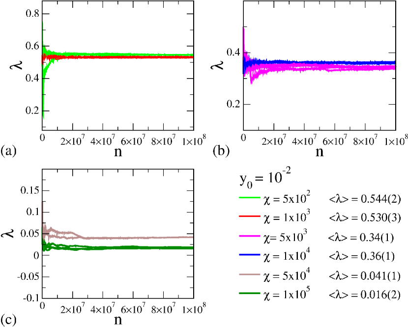
Figure 9: (Color online) Plot of the Lyapunov exponent averaged over the chaotic sea for mapping (4) considering the control parameter $y_{0}=0.01$ and: (a) $\chi=5\times 10^{2}$ and $\chi=1\times 10^{3}$ ; (b) $\chi=5\times 10^{3}$ and $\chi=1\times 10^{4}$; (c) $\chi=5\times 10^{4}$ and $\chi=1\times 10^{5}$.

shows the behavior of the Lyapunov exponent as a function of the collisions with the moving wall for the parameter $y_{0}=0.01$ and: (a) $\chi=5\times 10^{2}$ and $\chi=1\times 10^{3}$; (b) $\chi=5\times 10^{3}$ and $\chi=1\times 10^{4}$; (c) $\chi=5\times 10^{4}$ and $\chi=1\times 10^{5}$.

A possible explanation of the decrease of the Lyapunov exponent as an increase of the $\chi$ is due to the shape of the limit cycle. Indeed, for sufficiently small $\chi$, the shape of form of the limit cycle looks more like a sine function. However, as the parameter $\chi$ increases, the shape describing the motion of the moving wall has parts of large regularity, those where it moves slowly, and parts where it moves very fast. Therefore, we expected that, as the parameter $\chi$ increases, the particle suffers more collisions with the regular motion of moving wall. Eventually it collides with a region where the moving wall is moving very fast, therefore leading to a large exchange of energy, producing the regimes of growing velocities, as discussed before. Figure 10

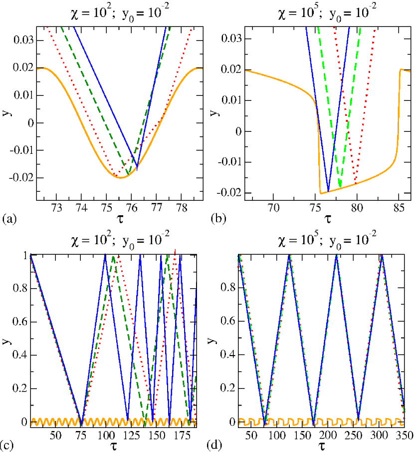
Figure 10: (Color online) Plot of the trajectory of the particle as a function of time. The parameters used were $y_{0}=10^{-2}$ and: (a) and (c) $\chi=10^{2}$ and; (b) and (d) $\chi=10^{5}$.

shows plots of the trajectory of the particle as a function of time. The parameters used were $y_{0}=10^{-2}$ and: (a) and (c) $\chi=10^{2}$ and; (b) and (d) $\chi=10^{5}$. One can see clearer that in (a) and (c), the separation of the two neighboring particles is more visible while compared to (b) and (d).

IV The case of $\mu\neq 0$

Let us consider in this section the case of $\mu\neq 0$. When the particle collides with the moving wall, it perturbs the motion of the moving wall, bringing it out/in the limit cycle. As the time evolves, the oscillator pushes the dynamics back to the limit cycle, restoring the dynamics. Under this circumstance, the mapping is now written as

$$v^{p}_{n+1} = \frac{\mu-1}{1+\mu}(v^{p}_{n}-v^{w}_{n})+v^{w}_{n},$$

$$v^{w}_{n+1} = \frac{2\mu}{1+\mu}(v^{p}_{n}-v^{w}_{n})+v^{w}_{n},$$

$$t_{n+1} = t_{n}+\Delta t_{n+1},$$

$$y_{n+1} = y_{w}(\phi_{n+1}).$$

where $v^{p}$ is the velocity of the particle, $v^{w}$ is the velocity of the moving wall, $\mu$ is the ratio of mass of the particle and mass of the wall, $t$ is the time, $y$ the position of the particle and $y^{w}$ is the position of the moving wall upon collision. The term $\Delta t_{n+1}$ is obtained as in the same way as made for the case of $\mu=0$ and is obtained numerically upon to an accuracy of $10^{-12}$.

The phase space is now defined by $(y,v,v_{w})$, i.e. the position of moving wall at the instant of the collision $y$, the velocity of the particle $v$ and the velocity of the moving wall $v_{w}$. Depending on the initial conditions and on the set of control parameters, the dynamics evolves to different fixed points, after passing by a transient. Therefore, we investigate the basin of attraction for the fixed points considering the parameters $\chi=10^{6}$, $y_{0}=0.001$ and $\mu=0.004$. The elliptic fixed points observed in the case $\mu=0$, turn into sinks after a bifurcation and initial conditions close enough converge to them asymptotically, a shown in Fig. 11.

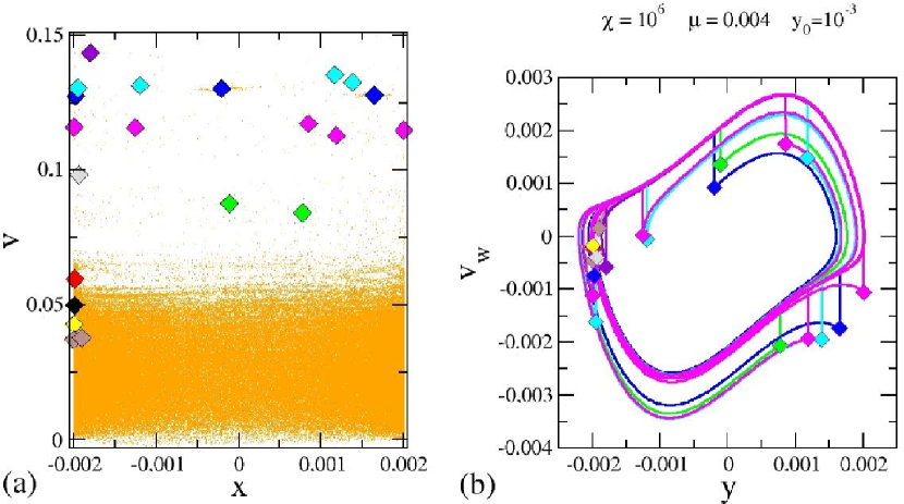
Figure 11: (Color online) Plot of the phase space $v~{}versus~{}x$. Square represents different attractors, yellow denotes the initial transient; (b) Phase space for the van der Pol oscillator when it is perturbed by collisions with the particle. Squares denote the instant of collision. The parameters used are $y_{0}=10^{-3}$, $\mu=0.004$ and $\chi=10^{6}$.

To construct a basin of attraction we set the initial conditions with the position of the moving wall along the limit cycle which is obtained from the numerical solution of the integration of the van der Pol oscillator. Thus the initial condition evolves in time until reaches a regime of convergence to different attractors. After analyzing the plots of the basin of attraction, we can identify several attractors with different periods as shown in Fig. 12.

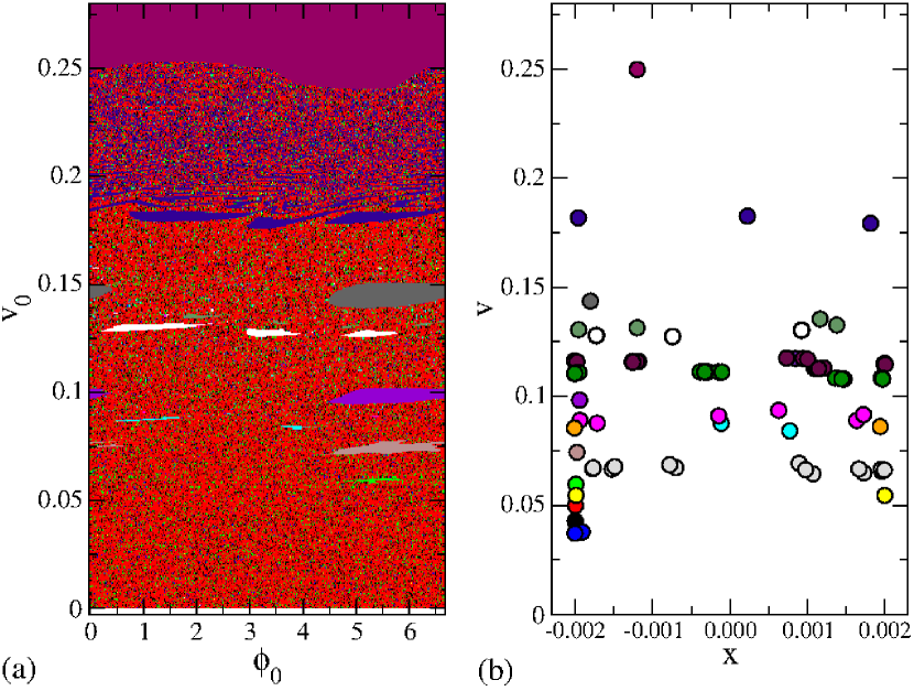
Figure 12: (Color online) (a) Basin of attraction $v_{0}~{}versus~{}\phi_{0}$; (b) Fixed points $v~{}verus~{}x$. The parameters used are $y_{0}=10^{-3}$, $\mu=0.004$ and $\chi=10^{6}$

Considering $v_{0}>0.25$ we found only attractors of period $1$. We can compare the basin of attraction with the phase space in case $\mu=0$ and note a series of similarities as for example, regions of periodic islands became regions that lead the dynamics to a periodic attractor as shown in Fig. 13.

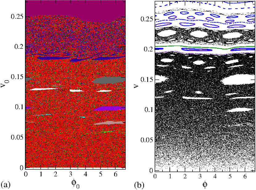
Figure 13: (Color online) (a) Basin of attraction $v_{0}~{}versus~{}\phi_{0}$ for the parameters $y_{0}=10^{-3}$, $\mu=0.004$ and $\chi=10^{6}$; (b) Phase space plot $v~{}verus~{}\phi$ for the parameters $y_{0}=10^{-3}$, $\mu=0.004$ and $\chi=0$.

The parameters used to construct Fig. 13 were: (a) $y_{0}=10^{-3}$, $\mu=0.004$ and $\chi=10^{6}$ and; (b) $y_{0}=10^{-3}$, $\mu=0.004$ and $\chi=0$. In the reference video2 a video is shown to demonstrate the dynamics of the system, compared the phase space of particle and the phase space of the moving wall.

We see from Figs. 12 and 13 that the basin of attraction for periodic orbits exhibit quite complicate organization. To have an estimate of how many initial conditions evolved to period 1, or period 2 and so on, we constructed a histogram of frequency of initial conditions that has as final state, a periodic attractor of period one, or two etc. We found that about $70\%$ of all initial conditions considered converge to the period 1 sink. The other periods from $2,3,4,5,6$ stay around $1\%$ and $10\%$ and some initial conditions lead to observe periods $20$ and $60$ as shown in Fig 14.

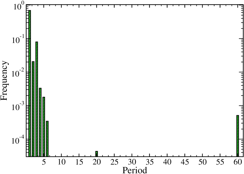
Figure 14: (Color online) Plot of the histogram of frequency of initial conditions for the period of the attractor. The parameters used are $y_{0}=10^{-3}$, $\mu=0.004$ and $\chi=10^{6}$.

The control parameters used in the figure were: $y_{0}=10^{-3}$, $\mu=0.004$ and $\chi=10^{6}$.

V Conclusion

We revisited and described the dynamics of a classical particle suffering elastic collisions with two walls. One is fixed and the other one is moving according to the solution of a van der Pool oscillator. The mapping describing the dynamics of the model was constructed considering the cases of: (i) the particle has negligible mass as compared to the mass of the moving wall and; (ii) the collisions of the particle affect the dynamics of the moving wall. Due to the properties of the van der Pol oscillator, after the collisions, the moving wall relaxes again to the limit cycle. We proposed an alternative method to calculate the average velocity of the particle along the phase space and, using it, we investigated the behavior of the average velocity of the particle. Scaling arguments were used to describe the behavior of the average velocity and critical exponents $\alpha=0.52(1)$, $\beta=1.2(3)$ and $z=-2.1(1)$ were used to overlap all curves of average velocity onto a single and seemingly universal plot. Lyapunov exponents were also discussed as a function of the control parameters.

For case (ii) in which the mass of the particle is taken into account along the collisions with the moving wall, the dynamics of the system changes and the system becomes dissipative leading to appearance of attractors in the dynamics. The basins of attraction of some attractors were obtained.

As a perspective of the study of this model with such type of perturbations, a synchronization of the oscillator may be of interest and applications may be used to control chaos. Other aspect of the model that can be studied is related to the introduction of two interacting particles in the system which exchange information through the perturbation caused by them in the moving wall.

VI ACKNOWLEDGMENTS

TB thanks CAPES and FAPESP. EDL kindly acknowledges the financial support from CNPq, FAPESP and FUNDUNESP, Brazilian agencies. EDL thanks the hospitality of the ICTP during his visit. T.B. also thanks Vinicius Santana, Roberto Eugenio Lagos Monaco and Tadashi Yokoyama for fruitful discussions. This research was supported by resources supplied by the Center for Scientific Computing (NCC/GridUNESP) of the São Paulo State University (UNESP).

References

- (1) E. Fermi, Phys. Rev. 75, 1169 (1949).
- (2) A. Veltri, V Carbone, Phys. Rev. Lett. 92, 143901, (2004).
- (3) K. Kobayakawa, Y. S. Honda, T. Samura, Phys. Rev. D 66, 083004, (2002).
- (4) A. V. Milovanov, L. M. Zelenyi, Phys. Rev. E 64, 052101 (2001).
- (5) F. Saif, I. Bialynicki-Birula, M. Fortunato, W. P. Schleich, Phys. Rev. A 58, 4779 (1998).
- (6) A. Steane, P. Szriftgiser, P. Desbiolles, J. Dalibard, Phys. Rev. Lett. 74, 4972, (1995).
- (7) G. Lanzano et al., Phys. Rev. Lett. 83, 4518, (1999).
- (8) A. Loskutov, A. B. Ryabov, J. Stat. Phys. 108, 995 (2002).
- (9) A. K. Karlis, P. K. Papachristou, F. K. Diakonos, V. Constantoudis and P. Schmelcher, Phys. Rev. Lett., 97, 194102 (2006).
- (10) A. K. Karlis, P. K. Papachristou, F. K. Diakonos, V. Constantoudis, P. Schmelcher, Phys. Rev. E 76, 016214 (2007).
- (11) A. K. Karlis, F. K. Diakonos and V. Constantoudis, “A consistent approach for the treatment of Fermi acceleration in time-dependent billiards”, To appear in Chaos (2012).
- (12) E. D. Leonel, J. of Phys. A, 40, F1077 (2007).
- (13) K. O. Menzel, O. Arp, A. Piel, Phys. Rev. Lett., 104, 235002 (2010).
- (14) K. O. Menzel, O. Arp, A. Piel, Phys. Rev. Lett., 84, 016405 (2011).
- (15) A. Bahraminasab, F. Ghasemi, A. Stefanovska, P. V. E. McClintock, and H. Kantz, Phys. Rev. Lett., 100, 084101 (2008).
- (16) P. Rosenau and A. Pikovsky, Phys. Rev. Lett., 94, 174102, (2005).
- (17) E. Everhart, An efficient integrator that uses Gauss-Radau spacings. In Dynamics of comets: Their origin and evolution, Eds. A. Carusi Carusi and G. B. Valsecchi, D.Reidel Publishing Company, (1985).
- (18) See Supplemental Material at [URL will be inserted by publisher] for video in which we compared the phase space of the particle and phase space of moving wall to case .
- (19) E. D. Leonel, P. V. E. McClintock and J. K. L. da Silva, Phys. Rev. Lett., 93, 014101 (2004).
- (20) F. Lenz, F. K. Diakonos, and P. Schmelcher, Phys. Rev. Lett., 100, 014103 (2008).
- (21) J. A. Méndez-Bermúdez and R. Aguilar-Sánchez, Phys. Rev. E, 85, 056212 (2012).
- (22) D. Wu and S. Zhu, Phys. Rev. E, 85, 061101 (2012).
- (23) A. Loskutov, A. Ryabov and, E. D. Leonel, Physica A, 389, 5408 (2010).
- (24) J. P. Eckmann and D. Ruelle, Rev. Mod. Phys., 57 (1985) 617.
- (25) See Supplemental Material at [URL will be inserted by publisher] for video in which we compared the phase space of the particle and phase space of moving wall to case .