Recovering the tree-like trend of evolution despite extensive lateral genetic transfer: A probabilistic analysis

Abstract

Lateral gene transfer (LGT) is a common mechanism of non-vertical evolution where genetic material is transferred between two more or less distantly related organisms. It is particularly common in bacteria where it contributes to adaptive evolution with important medical implications. In evolutionary studies, LGT has been shown to create widespread discordance between gene trees as genomes become mosaics of gene histories. In particular, the Tree of Life has been questioned as an appropriate representation of bacterial evolutionary history. Nevertheless a common hypothesis is that prokaryotic evolution is primarily tree-like, but that the underlying trend is obscured by LGT. Extensive empirical work has sought to extract a common tree-like signal from conflicting gene trees. Here we give a probabilistic perspective on the problem of recovering the tree-like trend despite LGT. Under a model of randomly distributed LGT, we show that the species phylogeny can be reconstructed even in the presence of surprisingly many (almost linear number of) LGT events per gene tree. Our results, which are optimal up to logarithmic factors, are based on the analysis of a robust, computationally efficient reconstruction method and provides insight into the design of such methods. Finally we show that our results have implications for the discovery of highways of gene sharing.

1 Introduction

High-throughput sequencing is transforming the study of evolution by allowing the integration of genome analysis and systematic studies, an area called phylogenomics [EF03, DBP05]. An important step in most phylogenomic analyses is the reconstruction of a tree of ancestor-descendant relationships—a gene tree—for each family of orthologous genes in a dataset. Such analyses have revealed widespread discordance between gene trees [GD08], leading some to question the meaningfulness of the Tree of Life [GDL02, ZLG04, GT05, BSL⁺05, DB07, Koo07]. In addition to statistical errors in gene tree estimation, various mechanisms commonly lead to incongruences between inferred gene histories, including hybridization events, duplications and losses in gene families, incomplete lineage sorting, and lateral genetic transfers [Mad97].

Here we study specifically lateral gene transfer (LGT), that is, the non-vertical transfer of genes between more or less distantly related organisms (as opposed to the standard vertical transmission between parent and offspring). Estimates of the fraction of genes that have undergone LGT vary widely—with some as high as 99%. See e.g. [DM06, GD08] and references therein. LGT is particularly common in bacterial evolution and it has been recognized to play an important role in microbial adaptation, selection and evolution with implications in the study of infectious diseases [SB05]. As a result, the bacterial phylogeny is usually inferred from genes that are thought to be immune to LGT, typically ribosomal RNA genes. However there is growing evidence that even such genes have in fact experienced LGT [YZW99, vBTP⁺03, SSJ03, DSS⁺05]. In any case, LGT appears to be a major source of conflict between gene trees that must be taken into account appropriately in phylogenomic analyses, in particular when building phylogenies. This is the problem we address in this paper.

Despite the confounding effect of LGT, we operate under the prevailing assumption that the evolution of organisms is governed primarily by vertical inheritance. In particular we ask:

1. How much genetic transfer can be handled before the tree-like signal is completely erased?

2. What phylogenetic reconstruction methods are most effective under this hypothesis?

These questions, and other related issues, have been the subject of some empirical and simulation-based work [BHR05, GWK05, Gal07, PWK09, PWK10, KPW11]. See also [GD08, RB09] for enlightening discussions. In particular there is ample evidence that a strong tree-like signal can be extracted in the presence of extensive LGT (although some debate remains on this question [GDL02]).

In this paper we provide the first (to our knowledge) mathematical analysis of the issues above. We work under a stochastic model of gene tree topologies positing that LGT events occur at more or less random locations on the species phylogeny [Gal07]. In our main result we establish quantitative bounds implying that surprisingly high levels of LGT—almost linear in the number of branches for each gene—can be handled by simple, computationally efficient inference procedures. That amount of genetic transfer appears to be much higher than known empirical estimates of LGT frequency based on genomic datasets in prokaryotes. Hence our results indicate that an accurate, reliable bacterial phylogeny should be reconstructible if the vertical inheritance hypothesis is correct. We prove that our bound on the achievable rate of LGT is tight up to logarithmic factors. We also show that constraining LGT to closely related species makes the tree reconstruction problem significantly easier.

Our theoretical approach complements simulation-based studies in allowing a broad range of parameters and tree shapes to be considered. Moreover our analysis provides new insights into the design of effective reconstruction methods in the presence of LGT. More precisely we focus on methodologies—both distance-based [KS01] and quartet-based [ZGC⁺06]—that derive their statistical power from the aggregation of basic topological information across genes.

In addition, we study the effect of so-called highways of gene sharing, roughly, preferred genetic exchanges between specific groups of species. Beiko et al. [BHR05] provided empirical evidence for the existence of such highways. To identify highways, they inferred LGT events by reconciling gene trees with a trusted species tree. In subsequent work, Bansal et al. [BBGS11] formalized the problem and designed a fast highway detection algorithm that aggregates conflicting signal across genes rather than solving the difficult LGT inference problem on each gene tree. Similarly to Beiko et al., Bansal et al. rely on a trusted species tree.

Here we show that a species phylogeny can be reliably estimated in the presence of both random LGT events and highways of LGT as long as such highways involve a small enough fraction of genes. Under extra assumptions, we also design an algorithm for inferring the location of highways. Because we first recover the species phylogeny, our highway reconstruction algorithm does not require a trusted species tree. In essence, our results on highways indicate that robust phylogeny reconstruction in the presence of random LGT extends to a phylogenetic network setting. For background on phylogenetic networks, see e.g. [HRS10].

We note that there exist related lines of work in phylogenomics addressing the issue of incomplete lineage sorting [DR09] in the presence of gene transfers and hybridization events [TRIN07, JML09, Kub09, MK09, YTDN11, CA11] as well as work on probabilistic models involving gene duplications and losses [ALS09, CM06].

The rest of the paper is organized as follows. In Section 2, we define a stochastic model of LGT and state our main results. A high-level description of our analysis is given in Section 3. Finally in Section 4 we extend our results to highways of gene sharing.

The results presented here were announced without proof in [RS12].

2 Model and Main Results

Before stating our main results, we present a stochastic model of LGT. Roughly, following Galtier [Gal07], we assume that LGT events occur more or less at random along the species phylogeny. Such a model appears to be consistent with empirical evidence [GD08].

Notation

Recall that, for functions $f(n),g(n)$, $f=O(g)$ means that there is constant $C>0$ such that $f(n)\leq Cg(n)$ for all $n$ large enough. Similarly, $f=\Omega(g)$ indicates $f(n)\geq C^{\prime}g(n)$ for $C^{\prime}>0$. In addition $f=\Theta(g)$ is equivalent to $f=O(g)$ and $f=\Omega(g)$. By polynomial in $n$, we mean $O(n^{C^{\prime\prime}})$ for some constant $C^{\prime\prime}>0$. We use the notation $\mathbb{P}[\mathcal{E}_{0}\,|\,\mathcal{E}_{1}]$ for the conditional probability of $\mathcal{E}_{0}$ given $\mathcal{E}_{1}$.

2.1 Stochastic Model of LGT

Gene trees and species phylogeny

A species phylogeny (or phylogeny for short) is a graphical representation of the speciation history of a group of organisms. The leaves correspond to extant or extinct species. Each branching indicates a speciation event. Moreover we associate to each edge a positive value corresponding to the time elapsed along that edge. For a tree $\mathcal{T}=(\mathcal{V},\mathcal{E})$ with leaf set $L$ and a subset of leaves $X\subseteq L$, we let $\mathcal{T}|X$ be the restriction of $\mathcal{T}$ to $X$, that is, the subtree of $\mathcal{T}$ where we keep only those vertices and edges on paths connecting two leaves in $X$. We say that $\mathcal{T}$ agrees (or is consistent) with $\mathcal{T}|X$.

Definition 1 (Phylogeny)

A (species) phylogeny $T_{s}=(V_{s},E_{s},L_{s};r,\tau)$ is a rooted tree with vertex set $V_{s}$, edge set $E_{s}$ and $n$ (labelled) leaves $L_{s}=[n]=\{1,\ldots,n\}$ such that 1) the degree of all internal vertices $V_{s}-L_{s}$ is exactly $3$ except the root $r$ which has degree $2$, and 2) the edges are assigned inter-speciation times $\tau:E_{s}\to(0,+\infty)$. We assume that $T_{s}$ includes $n^{+}>0$ extant species $L_{s}^{+}$ and $n^{-}\geq 0$ extinct species $L_{s}^{-}$, where $n=n^{+}+n^{-}$. We also associate to each edge $e\in E_{s}$ in $T_{s}$ a rate of lateral gene transfer $0<\lambda(e)<+\infty$. We denote by $T_{s}^{+}=(V_{s}^{+},E_{s}^{+},L_{s}^{+};r,\tau^{+})$, the subtree of $T_{s}$ restricted to the extant leaves $L_{s}^{+}$, that is, $T_{s}^{+}=T_{s}|L_{s}^{+}$ rooted at the most recent common ancestor of $L_{s}^{+}$. We further suppress vertices of degree $2$ in $T_{s}^{+}$ except the root (in which case we add up the branch lengths to obtain $\tau^{+}$). We call $T_{s}^{+}$ the extant phylogeny. We assume that $T_{s}^{+}$ is ultrametric, that is, from every node, the path lengths from that node to all its descendant leaves are equal.

Although we are ultimately interested in recovering the extant phylogeny, we include extinct species in the model as they can be involved in LGT events that affect the extant restriction of the tree. See e.g. [Mad97].

To infer the species phylogeny, we first reconstruct gene trees, that is, trees of ancestor-descendant relationships for orthologous genes or loci. Phylogenomic studies have revealed extensive discordance between such gene trees (e.g. [BSL⁺05, DB07]).

Definition 2 (Gene tree)

A gene tree $T_{g}=(V_{g},E_{g},L_{g};\omega_{g})$ for gene $g$ is an unrooted tree with vertex set $V_{g}$, edge set $E_{g}$ and $0<n_{g}\leq n$ (labelled) leaves $L_{g}\subseteq\{1,\ldots,n\}$ with $|L_{g}|=n_{g}$ such that 1) the degree of every internal vertex is either $2$ or $3$, and 2) the edges are assigned branch lengths $\omega_{g}:E_{g}\to(0,+\infty)$. We let $\mathcal{T}_{g}=\mathcal{T}[T_{g}]$ be the topology of $T_{g}$ where each internal vertex of degree $2$ is suppressed.

Remark 1 (Gene trees vs. species phylogeny)

As we will discuss below, gene trees are derived from— or “evolve” on—the species phlyogeny. They may differ from the species phylogeny for various reasons. First, in our model, their branch lengths represent expected numbers of substitutions, instead time elapsed. Moreover, their topology may differ as a result, in our case, of LGT events. See more details below.

Remark 2 (Rooted vs. unrooted)

Our stochastic model of LGT requires a rooted species phylogeny as time plays an important role in constraining valid LGT events. See, e.g., [JNST09]. In particular our results rely on the ultrametricity property of the extant phylogeny. In contrast, branch lengths in gene trees correspond to expected numbers of substitutions. As a result, gene trees are typically unrooted and do not satisfy ultrametricity.

Remark 3 (Taxon sampling)

Each leaf in a gene tree corresponds to an extant species in the species phylogeny. However, because of gene loss and taxon sampling, a taxon may not be represented in every gene tree.

Remark 4 (Branch lengths)

Each branch $e$ in a gene tree $T_{g}$ corresponds to a full or partial edge in the species phylogeny $T_{s}$. In particular, we allow internal vertices of degree $2$ in a gene tree to potentially delineate between two consecutive species edges. We allow the branch lengths $\omega_{g}(e)$ to be arbitrary, but one could easily consider cases where the branch lengths are determined by inter-speciation times, lineage-specific rates of substitution and gene-specific rates of substitution. The branch lengths will play a role in Section 5.

Random LGT

We formalize a stochastic model of LGT similar to Galtier’s [Gal07]. See also [KS01, Suc05, JNST06] for related models. The model accounts for LGT events originating at random locations on the species phylogeny with LGT rate $\lambda(e)$ prevailing along edge $e$.

We will need the following notation. Let $T_{s}=(V_{s},E_{s},L_{s};r,\tau)$ be a fixed species phylogeny. By a location in $T_{s}$, we mean any position along $T_{s}$ seen as a continuous object (also called $\mathbb{R}$-tree), that is, a point $x$ along an edge $e\in E_{s}$. We write $x\in e$ in that case. We denote the set of locations in $T_{s}$ by $\mathcal{X}_{s}$. For any two locations $x,y$ in $\mathcal{X}_{s}$, we let $\mathrm{MRCA}(x,y)$ be their most recent common ancestor (MRCA) in $T_{s}$ and we let $\tau(x,y)$ be the length of the path connecting $x$ and $y$ in $T_{s}$ under the metric naturally defined by the weights $\{\tau(e),e\in E_{s}\}$, interpolated linearly to locations along an edge. In words $\tau(x,y)$, which we refer to as the $\tau$-distance between $x$ and $y$, is the sum of times to $x$ and $y$ from $\mathrm{MRCA}(x,y)$. We say that two locations $x,y$ are contemporaneous if their respective $\tau$-distance to the root $r$ is identical, that is,

$$\tau(x,r)=\tau(y,r).$$

For $R>0$, we let

$$\mathcal{C}_{x}^{(R)}=\{y\in\mathcal{X}_{s}:\tau(r,x)=\tau(r,y),\ \tau(x,y)\leq 2R\}$$

be the set of locations contemporaneous to $x$ at $\tau$-distance at most $2R$ from $x$ (or in other words with MRCA at $\tau$-distance at most $R$). In particular, $\mathcal{C}_{x}^{(\infty)}$ denotes the set of all locations contemporaneous to $x$. We let $\Lambda(e)=\lambda(e)\tau(e)$, $e\in E_{s}$. We note that, since $\lambda(e)$ is the LGT rate on $e$, $\Lambda(e)$ gives the expected number of LGT events along $e$. Further, we let

$$\bm{\Lambda}_{\mathrm{tot}}=\sum_{e\in E_{s}}\Lambda(e),$$

be the total LGT weight of the phylogeny and

$$\bm{\Lambda}=\sum_{e\in\mathcal{E}(T_{s}|L_{s}^{+})}\Lambda(e),$$

be the total LGT weight of the extant phylogeny, where $\mathcal{E}(T_{s}|L_{s}^{+})$ denotes the edge set of $T_{s}|L_{s}^{+}$.

Our model of LGT is the following. Note first that, from a topological point of view, an LGT transfer is equivalent to a subtree-prune-and-regraft (SPR) operation [SS03]. The recipient location, that is, the location receiving the genetic transfer, is the point of pruning. Similarly, the donor location is the point of regrafting. In other words, on the gene tree, a new internal node is created at the donor location with two children nodes, one being the original endpoint of the corresponding edge and the other being the node immediately under the recipient location in the species phylogeny. The original edge going to the latter node is removed. See Figure 1.

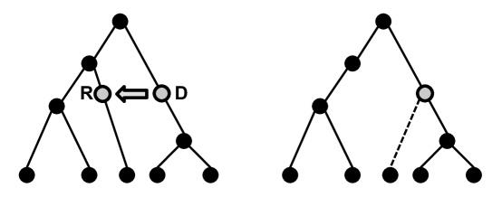
Figure 1: An LGT event. On the left, the species phylogeny is shown with the donor (D) and recipient (R) locations. On the right, the resulting (unweighted) gene tree is shown after the LGT transfer.

Definition 3 (Random LGT)

Let $0<R\leq+\infty$ possibly depending on $n$ (i.e. not necessarily a constant) and note that we explicitly allow $R=+\infty$. Let $T_{s}=(V_{s},E_{s},L_{s};r,\tau)$ be a fixed species phylogeny. Let $0<p\leq 1$ be a sampling effort probability. A gene tree topology $\mathcal{T}_{g}$ is generated according to the following continuous-time stochastic process which gradually modifies the species phylogeny starting at the root. There are two components to the process:

1. LGT locations. The recipient and donor locations of LGT events are selected as follows:

   • Recipient locations. Starting from the root, along each branch $e$ of $T_{s}$, locations are selected as recipient of a genetic tranfer according to a continuous-time Poisson process with rate $\lambda(e)$. Equivalently, the total number of LGT events is Poisson with mean $\bm{\Lambda}_{\mathrm{tot}}$ and each such event is located independently according to the following density. For a location $x$ on branch $e$, the density at $x$ is $\Lambda(e)/\bm{\Lambda}_{\mathrm{tot}}$.

   • Donor locations. If $x$ is selected as a recipient location, the corresponding donor location $y$ is chosen uniformly at random in $\mathcal{C}_{x}^{(R)}$. The LGT transfer is then obtained by performing an SPR move from $x$ to $y$, that is, the subtree below $x$ in $T_{s}$ is moved to $y$ in $T_{g}$. Note that we perform genetic transfers chronologically from the root.

2. Taxon sampling. Each extant leaf is kept independently with probability $p$. (One could also consider a different probability for each leaf. We use a fixed sampling effort $p$ for simplicity.) The set of leaves selected is denoted by $L_{g}$. The final gene tree $T_{g}$ is then obtained by keeping the subtree restricted to $L_{g}$.

The resulting (random) gene tree topology is denoted by $\mathcal{T}_{g}$.

When $R<+\infty$ a transfer can only occur between sufficiently closely related species. One could also consider more general donor location distributions. See e.g. [PWK10]. In Section 4, we consider a different form of preferential exchange, highways of gene sharing.

2.2 Recovering the tree-like trend: Main results

Problem statement

Let $T_{s}=(V_{s},E_{s},L_{s};r,\tau)$ be an unknown species phylogeny. Using homologous gene sequences for every gene at hand, we generate $N$ independent gene tree topologies $\mathcal{T}_{g_{1}},\ldots,\mathcal{T}_{g_{N}}$ as above. Given the gene trees (or their topologies), we seek to reconstruct the topology $\mathcal{T}_{s}^{+}=\mathcal{T}[T_{s}^{+}]$ of the extant phylogeny $T_{s}^{+}$. More precisely we are interested in the amount of LGT that can be sustained without obscuring the phylogenetic signal. To derive asymptotic results about this question, we make some assumptions on the underlying phylogeny. We discuss two cases in detail.

In practice, one estimates gene trees from sequence data. We come back to gene tree estimation issues below.

Bounded-rates model

The following assumption was introduced in [DR10] and is related to a common assumption in the mathematical phylogenetics literature.

Definition 4 (Bounded-rates model)

Let $0<\rho_{\lambda}<1$ and $0<\rho_{\tau}<1$ be constants. Let further $0<\overline{\tau}<+\infty$ be a constant and $0<\overline{\lambda}<+\infty$ be a value possibly depending on $n^{+}$. Under the Bounded-rates model, we consider the set of phylogenies $T_{s}=(V_{s},E_{s},L_{s};r,\tau)$ with $n^{+}>0$ extant leaves and $n^{-}\geq 0$ extinct leaves and extant phylogeny $T_{s}^{+}=(V_{s}^{+},E_{s}^{+},L_{s}^{+};r,\tau^{+})$ such that the following conditions are satisfied:

$$\underline{\lambda}\equiv\rho_{\lambda}\overline{\lambda}\leq\lambda(e)\leq\overline{\lambda},\quad\forall e\in E_{s},$$

and

$$\underline{\tau}\equiv\rho_{\tau}\overline{\tau}\leq\tau^{+}(e^{+})\leq\overline{\tau},\quad\forall e^{+}\in E_{s}^{+}.$$

Our result in this case is the following. We use $\overline{\lambda}$ to control the amount of LGT in the model.

Theorem 1 (Main result: Bounded-rates model, $R=+\infty$)

Let $R=+\infty$. Under the Bounded-rates model, it is possible to reconstruct the topology of the extant phylogeny with high probability (w.h.p.) from $N=\Omega(\log n^{+})$ gene tree topologies if $\overline{\lambda}$ is such that

$$\bm{\Lambda}=O\left(\frac{n^{+}}{\log n^{+}}\right).$$

In words, we can reconstruct the species phylogeny w.h.p. as long as the expected number of LGT events $\bm{\Lambda}$ (as measured on the extant phylogeny) per gene is at most of the order of $\frac{n^{+}}{\log n^{+}}$. This result is based on a polynomial-time algorithm we describe in Section 3. Note that, in typical phylogenomic studies, the number of genes is much larger than the number of species. Therefore, our assumption that the number of genes should be at least of the order of the logarithm of the number of extant species is mild.

We also show that the bound on $\bm{\Lambda}$ in Theorem 1 is close to optimal, up to logarithmic factors.

Theorem 2 (Non-recoverability)

Under the Bounded-rates model as above with $N=O(\log n^{+})$, the topology of the extant phylogeny cannot, in general, be reconstructed w.h.p. if $\overline{\lambda}$ is such that $\bm{\Lambda}=\Omega(n^{+}\log\log n^{+})$.

More generally, the species phylogeny cannot be reconstructed from $N$ genes if $\bm{\Lambda}=\Omega(n^{+}\log N)$. Theorem 2 is proved by a coupling argument [Lin92]. In words we show that, with the order of $\Omega(n^{+}\log\log n^{+})$ expected LGT events, there is insufficient signal from the gene trees to distinguish between two species phylogenies with high probability.

Yule process

Branching processes are commonly used to model species phylogenies [RY96]. In the continuous-time Yule process (or pure-birth process), one starts with two species (representing the two branches emanating from the root). At any given time, each species generates a new offspring at rate $0<\nu<+\infty$. We stop the process when the number of species is exactly $n+1$ (and ignore the $n+1$st species). This process generates a species phylogeny with $n=n^{+}$ extant species with branch lengths given by the inter-speciation times in the above process. Note that $n^{-}=0$ by construction. Let $0<\rho_{\lambda}<1$ be a constant. We also assume that

$$\underline{\lambda}\equiv\rho_{\lambda}\overline{\lambda}\leq\lambda(e)\leq\overline{\lambda},\quad\forall e\in E_{s},$$

for some $0<\overline{\lambda}<+\infty$ possibly depending on $n$. As above, we use $\overline{\lambda}$ to control the amount of LGT in the model.

An advantage of the Yule model is that, unlike the Bounded-rates model, it does not place arbitrary constraints on the inter-speciation times. In particular, the following analog of Theorem 1 suggests that our analysis does not rely on such constraints.

Theorem 3 (Main result: Yule process, $R=+\infty$)

Let $R=+\infty$. Under the Yule model, the following holds with probability arbitrarily close to $1$. It is possible to reconstruct the topology of the extant phylogeny w.h.p. from $N=\Omega(\log n)$ gene tree topologies if $\overline{\lambda}$ is such that

$$\bm{\Lambda}=O\left(\frac{n}{\log n}\right).$$

Preferential LGT

When $R<+\infty$, that is, when transfers occur only between sufficiently related species, we obtain the following generalization which implies that preferential LGT makes the tree-building problem easier.

Theorem 4 (Preferential LGT)

Let $0<R<\log n^{+}$ possibly depending on $n^{+}$. Under the Bounded-rates model, it is possible to reconstruct the topology of the extant phylogeny w.h.p. from $N=\Omega(\log n^{+})$ gene tree topologies if $\overline{\lambda}$ is such that

$$\bm{\Lambda}=O\left(\frac{n^{+}}{R}\right).$$

A similar result holds under the Yule model.

Further results

We also obtain results on highways of LGT as well as sequence-length requirements. These results require additional background. See Sections 4 and 5 respectively.

3 Probabilistic Analysis

We assume that we are given $N$ independent gene tree topologies $\mathcal{T}_{g_{1}},\ldots,\mathcal{T}_{g_{N}}$ as above. Our goal is to reconstruct the extant phylogeny.

Different algorithms are possible. A simple approach is to take a majority vote over all gene tree topologies. But this approach is problematic under taxon sampling and cannot sustain the high levels of LGT we consider below.

Instead we consider approaches that aggregate partial information over all gene trees. We focus on subtrees over four taxa whose topologies are called quartets [SS03]. We show that computationally efficient quartet-based approaches can sustain high levels of LGT. Although we prove our results for the specific method described below, our analysis is likely to apply to related methods. In Section 5.1, we also give a similar analysis for a distance-based method of Kim and Salisbury [KS01].

3.1 Algorithm

We consider the following approach related to an algorithm of Zhaxybayeva et al. [ZGC⁺06]. Let $X=\{a,b,c,d\}$ be a four-tuple of extant species The topology $\mathcal{T}|X$ of a tree $\mathcal{T}$ restricted to $X$ can be summarized with a quartet split, or quartet for short. There are three possible (resolved) quartets which we denote $q_{1}=ab|cd$, $q_{2}=ac|bd$, and $q_{3}=ad|bc$. We first compute the frequency of each quartet over all gene trees displaying $X$, that is, over all gene trees $g$ such that $X\subseteq L_{g}$,

$$f_{X}(q_{1})=\frac{|\{g_{i}:X\subseteq L_{g_{i}},\ \mathcal{T}_{g_{i}}|X=q_{1}\}|}{|\{g_{i}:X\subseteq L_{g_{i}}\}|},$$

and similarly for $q_{2},q_{3}$. (We set the frequency to $0$ if the denominator is $0$.) For each $X$, we choose the quartet with highest frequency (breaking ties arbitrarily).

Definition 5

A set of quartets $Q=\{q_{i}\}$, with $L_{q_{i}}$ the leaf set of $q_{i}$, is compatible if there is a tree ${\cal T}$ with leaf set $L_{Q}\equiv\cup_{q_{i}\in Q}L_{q_{i}}$ such that ${\cal T}$ agrees with every $q_{i}$.

Quartet compatibility is, in general, NP-hard [Ste92]. However, when the set $Q$ covers all possible four-tuple of taxa (that is, exactly $n\choose 4$ quartets with no repeated four-tuple of taxa), there is a polynomial-time algorithm for compatibility [BD86, Bun71, BG01]. In our procedure, for every four-tuple of taxa, there is a single quartet chosen, so we can check compatibility easily and output the corresponding tree. In practice, if $Q$ is not compatible, one can use instead a heuristic supertree method such as MRP [Rag92, Bau92] or Quartet MaxCut [SR10, SR12].

The algorithm, which we call QuartetPlurality (QP), is detailed in Figure 6.

Algorithm QuartetPlurality
Input: Gene trees $g_{1},\ldots,g_{N}$;
Output: Estimated species phylogeny $\hat{T}$; • Set $Q=\emptyset$ • For all four-tuple of taxa $X=\{a,b,c,d\}$, letting $q_{1}=ab|cd$, compute $$f_{X}(q_{1})=\frac{|\{g_{i}:X\subseteq L_{g_{i}},\ \mathcal{T}_{g_{i}}|X=q_{1}\}|}{|\{g_{i}:X\subseteq L_{g_{i}}\}|},$$ and similarly for $q_{2}=ac|bd$ and $q_{3}=ad|bc$. Add the quartet with highest frequency (breaking ties arbitrarily) to $Q$. • Using Buneman’s algorithm [Bun71] compute the tree $\hat{T}$ compatible with $Q$ (or abort if no such tree is found). • Output $\hat{T}$.

Figure 2: Algorithm QuartetPlurality.

3.2 A general formula

Our asymptotic analysis is based on the following claim. Recall that, for a subset of extant species $X$, we let $\mathcal{T}_{s}|X$ be the extant phylogeny topology restricted to $X$ with corresponding edge set $\mathcal{E}(\mathcal{T}_{s}|X)$. Also recall that $\Lambda(e)=\lambda(e)\tau(e)$ is the expected number of LGT events on edge $e$ which we refer to as the LGT weight, or weight for short, of $e$. Let

$$\bm{\Lambda}_{X}=\sum_{e\in\mathcal{E}(\mathcal{T}_{s}|X)}\Lambda(e),$$

be the total weight of the subtree $\mathcal{T}_{s}|X$ under the weights $\Lambda(e)$, $e\in E_{s}$. Define the maximum quartet weight (MQW) as

$$\bm{\Upsilon}^{(4)}=\max\{\bm{\Lambda}_{X}:X\subseteq(L_{s}^{+})^{4}\}.$$

Lemma 1 (Probability of a miss)

Let $\mathcal{T}_{g}$ be a gene tree topology distributed according to the random LGT model such that $X=\{a,b,c,d\}\subseteq L_{g}$. Let $q^{X}_{s}$ (respectively $q^{X}_{g}$) be the quartet corresponding to $\mathcal{T}_{g}|X$ (respectively $\mathcal{T}_{s}|X$). Then

$$\mathbb{P}[q^{X}_{g}=q^{X}_{s}|X\subseteq L_{g}]\geq\exp\left(-\bm{\Upsilon}^{(4)}\right).$$

Recall that $\bm{\Lambda}$ is the expected number of LGT events (as measured on the extant phylogeny) per gene. As a comparison, note that the probability that a gene tree is LGT-free is $e^{-\bm{\Lambda}}$, which can be much smaller.

Proof (Lemma 1): We first note that, by our assumption that the species phylogeny is bifurcating, $q^{X}_{s}$ is resolved. Similarly $q^{X}_{g}$ is resolved because under a Poisson process for the recipient location the probability that a vertex has degree higher than $2$ (that is, that a pruning and re-grafting occurs exactly at the location of an existing vertex) is $0$.

Now we observe that if none of the recipient locations lands on $\mathcal{T}_{s}|X$ then the corresponding quartet remains intact. Indeed an SPR move can only (potentially) affect those quartets with at least one leaf in the pruned subtree, and this happens with probability $\frac{\bm{\Lambda}_{X}}{\bm{\Lambda}}$. The claim then follows by induction on the number of LGT events.

Hence the probability that $q^{X}_{g}=q^{X}_{s}$ is at least the probability that all LGT events (on the extant phylogeny) miss $\mathcal{T}_{s}|X$, which is at least

$$\mathbb{P}[q^{X}_{g}=q^{X}_{s}|X\subseteq L_{g}] \geq \sum_{i=0}^{+\infty}\frac{e^{-\bm{\Lambda}}\bm{\Lambda}^{i}}{i!}\left(1-\frac{\bm{\Lambda}_{X}}{\bm{\Lambda}}\right)^{i}$$

$$= e^{-\bm{\Lambda}}\exp\left(\bm{\Lambda}\left(1-\frac{\bm{\Lambda}_{X}}{\bm{\Lambda}}\right)\right)$$

$$\geq \exp\left(-\bm{\Upsilon}^{(4)}\right).$$

$\blacksquare$

3.3 Bounded-rates and Yule models

Next we argue that, under appropriate assumptions on the species phylogeny, the maximum quartet weight is bounded in such a way that the plurality quartet topology for every four-tuple of taxa $X=\{a,b,c,d\}$, which we denote by $q^{X}_{*}$, satisfies $q^{X}_{*}=q^{X}_{s}$. As a result, our quartet set is compatible and $\mathcal{T}_{s}^{+}$ can be reconstructed efficiently.

3.3.1 Bounded-rates model

We bound the maximum quartet weight $\bm{\Upsilon}^{(4)}$ in the Bounded-rates model.

Lemma 2 (Bound on quartet weight: Bounded-rates case)

Under the Bounded-rates model it holds that

$$\bm{\Upsilon}^{(4)}=O\left(\overline{\lambda}\log n^{+}\right),\qquad\bm{\Lambda}=\Theta(\overline{\lambda}n^{+}).$$

Proof (Lemma 2): The first part of the proof is taken from [DR10]. Let $h$ (respectively $H$) be the smallest (respectively largest) number of edges on a path between the root and an extant leaf. Because the number of extant leaves is $n^{+}$ and the extant phylogeny is bifurcating (recall that we suppressed vertices of degree $2$ after taking a restriction to the extant species), we must have $2^{h}\leq n^{+}$ and $2^{H}\geq n^{+}$. Since all extant leaves are contemporaneous it must be that $H\underline{\tau}\leq h\overline{\tau}$. Combining these constraints gives

$$\frac{\underline{\tau}}{\overline{\tau}}\log_{2}n^{+}\leq h\leq H\leq\frac{\overline{\tau}}{\underline{\tau}}\log_{2}n^{+}.$$

Hence

$$\max\{\bm{\Lambda}_{X}:X\subseteq(L_{s}^{+})^{4}\}\leq 4\overline{\lambda}\overline{\tau}\frac{\overline{\tau}}{\underline{\tau}}\log_{2}n^{+}.$$

The total number of edges in the extant phylogeny is $2n^{+}-3$ so that

$$\bm{\Lambda}=\Theta(\overline{\lambda}n^{+}).$$

$\blacksquare$

Using Lemma 2, we prove Theorem 1. First recall the following standard concentration inequality (see e.g. [MR95]):

Lemma 3 (Azuma-Hoeffding Inequality)

Suppose ${\bf Z}=(Z_{1},\ldots,Z_{m})$ are independent random variables taking values in a set $S$, and $h:S^{m}\to\mathbb{R}$ is any $t$-Lipschitz function: $|h(\mathbf{z})-h(\mathbf{z^{\prime}})|\leq t$ whenever $\mathbf{z},\mathbf{z^{\prime}}\in S^{m}$ differ at just one coordinate. Then, $\forall\zeta>0$,

$$\mathbb{P}\left[|h({\bf Z})-\mathbb{E}[h({\bf Z})]|\geq\zeta\right]\leq 2\exp\left(-\frac{\zeta^{2}}{2t^{2}m}\right).$$

Proof (Theorem 1): Consider the quartet-based approach described in Section 3.1. Take $\overline{\lambda}=C_{1}/\log n^{+}$ with $C_{1}>0$ small enough so that

$$\bm{\Lambda}=O\left(\frac{n^{+}}{\log n^{+}}\right),$$

and using Lemmas 1 and 2, we have for any four-tuple $X$ of extant species

$$\mathbb{P}[X\subseteq L_{g}]=p^{4},$$

and

$$\mathbb{P}[q^{X}_{g}=q^{X}_{s}\,|\,X\subseteq L_{g}]\geq\exp\left(-\bm{\Upsilon}^{(4)}\right)\geq\exp\left(-O(C_{1})\right)\geq\frac{2}{3},$$

for $C_{1}$ small enough. We choose $C_{2}>0$ large enough with

$$N\geq C_{2}\log n^{+},$$

and $\varepsilon<p^{4}$ so that, using Lemma 3, the following inequalities hold. Consider the following events

$$\mathcal{E}_{0}=\{||\{g_{i}:X\subseteq L_{g_{i}}\}|-Np^{4}|\leq N\varepsilon\}$$

and

$$\mathcal{E}_{1}=\left\{|\{g_{i}:X\subseteq L_{g_{i}},\ \mathcal{T}_{g_{i}}|X=q_{1}\}|>\frac{1}{2}|\{g_{i}:X\subseteq L_{g_{i}}\}|\right\}.$$

By Lemma 3,

$$\mathbb{P}[\mathcal{E}_{0}^{c}]\leq\exp\left(-O(\varepsilon^{2}N)\right),$$

and

$$\mathbb{P}[\mathcal{E}_{1}^{c}\,|\,\mathcal{E}_{0}]\leq\exp\left(-O(N(p^{4}-\varepsilon))\right).$$

Hence, for a constant $C_{2}$ large enough,

$$\mathbb{P}[f_{X}(q^{X}_{s})<1/2] \leq \mathbb{P}[\mathcal{E}_{0}^{c}]+\mathbb{P}[\mathcal{E}_{1}^{c}\,|\,\mathcal{E}_{0}]$$

$$\leq O\left(\frac{1}{(n^{+})^{4}}\right).$$

Then the plurality vote is correct for every four-tuple of taxa and the extant phylogeny is correctly reconstructed. $\blacksquare$

3.3.2 Yule process

We now consider the Yule model.

Lemma 4 (Bound on quartet weight: Yule case)

Under the Yule model, it holds that

$$\bm{\Upsilon}^{(4)}=\Theta\left(\overline{\lambda}\log n\right),\qquad\bm{\Lambda}=\Theta\left(\overline{\lambda}n\right)$$

with probability approaching $1$ as $n\to+\infty$.

Proof (Lemma 4): We consider a pure-birth process with birth rate $\nu$ starting from $2$ species. For background on branching processes see [AN72].

Let $Z_{i}$ be the $(i-1)$-th inter-speciation time. As a minimum of $i$ independent exponential distributions with mean $1/\nu$, $Z_{i}$ is an exponential with mean $1/(i\nu)$. Moreover the $Z_{i}$s are independent. Hence the height of the phylogeny in time units, that is, the total time until $n+1$ species are present (recall that we ignore the $(n+1)$-st species) is

$${\bf Z}=\sum_{i=2}^{n+1}Z_{i},$$

and we have

$$\mathbb{E}[{\bf Z}]=\sum_{i=2}^{n+1}\mathbb{E}[Z_{i}]=\sum_{i=2}^{n+1}\frac{1}{i\nu}=\Theta(\nu^{-1}\log n),$$

and

$$\mathrm{Var}[{\bf Z}]=\sum_{i=2}^{n+1}\mathrm{Var}[Z_{i}]=\sum_{i=2}^{n+1}\frac{1}{i^{2}\nu^{2}}=\Theta(\nu^{-2}).$$

The total weight of the phylogeny in time units

$${\bf Y}=\sum_{i=2}^{n+1}iZ_{i},$$

is a sum of $n$ independent exponential random variables with parameter $\nu$, and we have

$$\mathbb{E}[{\bf Y}]=\sum_{i=2}^{n+1}i\mathbb{E}[Z_{i}]=\sum_{i=2}^{n+1}i\frac{1}{i\nu}=\nu^{-1}n,$$

and

$$\mathrm{Var}[{\bf Y}]=\sum_{i=2}^{n+1}i^{2}\mathrm{Var}[Z_{i}]=\sum_{i=2}^{n+1}i^{2}\frac{1}{i^{2}\nu^{2}}=\nu^{-2}n.$$

By Chebyshev’s inequality,

$$\mathbb{P}[{\bf Z}\geq C_{1}\log n]\leq\frac{C_{2}}{C_{3}\log^{2}n}\to 0,$$

and

$$\mathbb{P}[{\bf Y}\leq C_{4}n]\leq\frac{C_{5}n}{C_{6}n^{2}}\to 0,$$

for appropriately chosen $C$s not depending on $n$. The same holds in the other direction so that $\bm{\Upsilon}^{(4)}=\Theta(\overline{\lambda}\log n)$ and $\bm{\Lambda}=\Theta(\overline{\lambda}n)$ with probability approaching $1$. $\blacksquare$

Proof (Theorem 3): Using Lemma 4, the proof of Theorem 3 follows form the same lines as that of Theorem 1. $\blacksquare$

3.4 Preferential LGT

We now prove Theorem 4.

Proof (Theorem 4): The proof is similar to that of Theorems 1 and 3. The main difference is in the proof of Lemma 1. In that proof, note that if $R<+\infty$ then for an LGT to affect the quartet on $X$, it must be that not only 1) the recipient location lands on $\mathcal{T}_{s}|X$, but also 2) that it lands on a location below either branchings of the corresponding quartet tree within time $R$ of the branching point. Indeed these are the only locations where the corresponding leg of the quartet tree can potentially jump to a subtree corresponding to a different leg. (In fact, it must be that a leg on the other side of the internal branch of the quartet tree is within time $2R$.) The length of this region is at most $4R$ in $\tau$-distance. Hence in the bound on the probability of a miss we get

$$\mathbb{P}[q^{X}_{g}=q^{X}_{s}|X\subseteq L_{g}] \geq \exp\left(-\min\{\bm{\Upsilon}^{(4)},4R\overline{\lambda}\}\right).$$

The result then follows. $\blacksquare$

3.5 Non-recoverability

We now prove Theorem 2.

Proof (Theorem 2): We use a coupling argument [Lin92]. Fix $\delta>0$ small. We construct two species phylogenies with different topologies which cannot be distinguished with probability $1-\delta$ from $N$ gene tree topologies when the total expected amount of LGT $\bm{\Lambda}$ is of the order of $n^{+}\log\log n^{+}$ per gene. In particular the reconstruction problem cannot be solved in that case. The idea of a coupling is to run the stochastic processes of LGT on both phylogenies simultaneously so as to output the same gene trees with high probability without changing the marginal distributions (that is, the probability distributions of gene tree topologies on each phylogeny separately).

We proceed as follows. Consider a complete binary tree $T_{s}^{\prime}$ on a set of $n$ leaves (all extant) and denote the four children at height 2 from the root as $a,b,c,d$, where $a$ and $b$ are sisters and so are $c$ and $d$. Let $T_{z}$ be the subtree with $n/4$ leaves rooted at $z\in\{a,b,c,d\}$. Moreover, for simplicity, assume all edges of $T_{s}^{\prime}$ have the same LGT weight. From $T_{s}^{\prime}$ we construct $T_{s}^{\prime\prime}$ by rewiring the four nodes $\{a,b,c,d\}$ such that $a$ is now sister with $c$ and $b$ with $d$.

We generate $N=\Theta(\log n)$ genes trees on each of $T_{s}^{\prime}$ and $T_{s}^{\prime\prime}$ as follows. We run the stochastic process of LGT on $T_{s}^{\prime}$ as described in Definition 3. Let $\mathcal{T}_{g_{1}}^{\prime},\ldots,\mathcal{T}_{g_{N}}^{\prime}$ be the gene tree topologies so obtained. For $T_{s}^{\prime\prime}$ and every gene, we use exactly the same LGT events as the ones generated on $T_{s}^{\prime}$ where we identify the two edges adjacent to the roots in $T_{s}^{\prime}$ and $T_{s}^{\prime\prime}$ arbitrarily. Let $\mathcal{T}_{g_{1}}^{\prime\prime},\ldots,\mathcal{T}_{g_{N}}^{\prime\prime}$ be the gene tree topologies so obtained.

Since $T_{s}^{\prime}$ and $T_{s}^{\prime\prime}$ are identical below every $z\in\{a,b,c,d\}$ and LGT events occur only between contemporaneous points, the subtrees under $\{a,b,c,d\}$ in $\mathcal{T}_{g_{i}}^{\prime}$ and $\mathcal{T}_{g_{i}}^{\prime\prime}$ are identical for every gene $i$.

For $z\in Z$, let $e_{z}$ be the edge adjacent to $z$ and above it in $T_{s}^{\prime}$ (and in $T_{s}^{\prime\prime}$). It remains to show that, for $\mathcal{T}_{g_{i}}^{\prime}$ and $\mathcal{T}_{g_{i}}^{\prime\prime}$ to be identical under the joint construction above, it suffices that the following good event occurs: three consecutive LGT moves start on the same edge in $e_{a},\ldots,e_{d}$ (donor location) and land on the other three edges in $e_{a},\ldots,e_{d}$ (recipient location), for example, $a\rightarrow d$, $a\rightarrow c$, $a\rightarrow b$. See Figure 3.

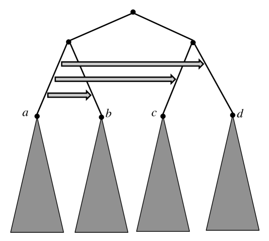
Figure 3: Good event.

Indeed, in that case, the first donor location above becomes the common ancestor to all nodes in the gene trees. From that point on, we obtain the same gene tree for both phylogenies.

We claim that the probability that the good event does not occur is $O(1/\log n)$. Under the assumption that $\bm{\Lambda}=\Omega(n\log\log n)$ and that the LGT weights are equal, the number of LGT events on any edge is Poisson with mean $\Omega(\log\log n)$. Consider the time interval between the nodes at height $1$ from the root and the nodes at height $2$. Divide this interval into $\nu=O(\log\log n)$ equal subintervals $I_{1},\ldots,I_{\nu}$ such that the number of LGT events on edge $e_{z}$ in $I_{i}$ is Poisson with mean $C_{0}$ for some constant $C_{0}>0$. In $I_{i}$ the probability that there is no LGT event originating from $e_{b},\ldots,e_{d}$ and that there is exactly three LGT events originating from $e_{a}$ and landing on $e_{b},e_{c},e_{d}$ in that order is

$$\tilde{p}=\left(e^{-C_{0}}\right)^{3}\left(e^{-C_{0}}\frac{C_{0}^{3}}{3!}\left(\frac{1}{3}\right)^{3}\right)\equiv C_{1}.$$

The subintervals are independent. The probability that the event above does not happen in any of $I_{1},\ldots,I_{\nu}$, is

$$\tilde{p}^{\nu}=(1-C_{1})^{\nu}=O\left(\frac{1}{\log n}\right).$$

This gives an upper bound of $O(1/\log n)$ on the probability that the good event does not happen.

Therefore, by a union bound over the genes, the probability that the good event does not occur on at least one gene tree is $\Theta(\log n)\cdot O(1/\log n)=O(1)$, which is at most $\delta$ if the constant in $\bm{\Lambda}$ is large enough. If the good event occurs on every gene tree, then both phylogenies output the exact same set of gene tree topologies. That concludes the proof. $\blacksquare$

4 Highways of LGT

In this section, we add highways of gene sharing to the model. Highways are, in essence, non-random patterns of LGT [BHR05]. These can potentially take different shapes. Following Bansal et al. [BBGS11], we focus on pairs of edges in the phylogeny that undergo an unusually large number of LGT events between them.

We give two results. As long as the frequency of genes affected by highways is low enough, the species phylogeny can be reconstructed using the same approach as in Section 3. Moreover, with extra assumptions on the positions of the highways with respect to each other, the highways themselves can be inferred.

In this section, we assume $n^{-}=0$.

4.1 Model

We generalize our model of LGT as follows.

Definition 6 (Highways of LGT)

Let $T_{s}=(V_{s},E_{s},L_{s};r,\tau)$ be a species phylogeny with LGT rates $0<\lambda(e)<+\infty$, $e\in E_{s}$ and let $0<p\leq 1$ be a taxon sampling probability. Assume $n^{-}=0$. For $\beta=1,\ldots,B$, let $\mathbf{H}_{\beta}=(e^{H}_{\beta,0},e^{H}_{\beta,1})$ be a pair of edges in $T_{s}$ which share contemporaneous locations. We call $\mathbf{H}_{\beta}$ a highway. Let $g_{1},\ldots,g_{N}$ be $N$ genes. Each highway $\mathbf{H}_{\beta}$ involves a subset $\mathbf{G}^{H}_{\beta}$ of the genes. If gene $g_{i}\in\mathbf{G}^{H}_{\beta}$, then it undergoes an LGT event between a pair of contemporaneous locations $x^{H}_{\beta,i}\in e^{H}_{\beta,0}$ and $y^{H}_{\beta,i}\in e^{H}_{\beta,1}$. We let $\gamma_{\beta}$ be the fraction of genes such that $g_{i}\in\mathbf{G}^{H}_{\beta}$ and we assume that $\gamma_{\beta}>\underline{\gamma}$ for some $\underline{\gamma}$ (chosen below). In addition, independently from the above, we assume that each gene undergoes LGT events at random locations as described in Definition 3. We denote by $\mathcal{T}_{g_{1}},\ldots,\mathcal{T}_{g_{N}}$ the gene tree topologies so obtained.

Remark 5 (Deterministic setting)

Note that the highways and which genes are involved in them are deterministic in this setting. Only the random LGT events are governed by a stochastic process. Note moreover that we allow highway events to go in either direction, that is, from $e^{H}_{\beta,0}$ to $e^{H}_{\beta,1}$ or vice versa.

4.2 Building the species tree in the presence of highways

We first prove that the species phylogeny can still be reconstructed in the presence of highways as long as the fraction of genes involved in highways is low enough. We only discuss the Bounded-rates model with $R=+\infty$.

Theorem 5 (Highways of LGT)

Consider the Bounded-rates model with $R=+\infty$ and assume that $B<+\infty$ is constant. Assume further that there is a constant $0<\overline{\gamma}<1$ such that

$$\gamma_{\beta}<\overline{\gamma},\quad\beta=1,\ldots,B.$$

If

$$\overline{\gamma}<\frac{1}{2B},$$

then it is possible to reconstruct the topology of the extant phylogeny w.h.p. from $N=\Omega(\log n^{+})$ gene tree topologies if $\overline{\lambda}$ is such that

$$\bm{\Lambda}=O\left(\frac{n^{+}}{\log n^{+}}\right).$$

Proof (Theorem 5): The proof is similar to that of Theorem 1. Note that a quartet tree in the species phylogeny can be affected by a highway in at most a fraction $<B\frac{1}{2B}=\frac{1}{2}$ of the genes. Moreover by the proof of Lemma 1, choosing $C_{1}$ small enough, a quartet tree is affected by a random LGT event in an arbitrarily small fraction of genes. Therefore the plurality vote will reconstruct the correct split with high probability. The result follows. $\blacksquare$

4.3 Inferring highways

The problem of inferring the highway locations is essentially a network reconstruction problem. Such problems are often computationally intractable. See e.g. [HRS10]. Therefore, we require some extra assumptions. Our goal here is not to provide the most general result but rather to illustrate that our analysis extends naturally to certain network settings. The following assumption is related to so-called galled trees.

Assumption 1

We assume that no highway connects two edges in $T_{s}$ separated by less than two edges or edges adjacent to root edges. (Such cases cannot be reconstructed.) Seen as an edge superimposed on $T_{s}$, a highway event $(x^{H}_{\beta,i},y^{H}_{\beta,i})$ forms a cycle. We assume that all such cycles are disjoint, that is, they do not share common locations.

We then prove the following. We use a computationally efficient algorithm, which we call RoadRoller, described in Figure 4 and explained in the proof.

Algorithm RoadRoller
Input: Gene trees $g_{1},\ldots,g_{N}$;
Output: Estimated species phylogeny $\hat{T}$ and highway locations; • Use QuartetPlurality to reconstruct the species phylogeny $\hat{T}$. Let $\mathcal{Q}$ be the set of all quartets whose estimated frequency is less than $1/2$ but more than $\underline{\gamma}/2$. • For all pairs of four-tuples $X\neq X^{\prime}$ (possibly sharing taxa) with a corresponding quartet in $\mathcal{Q}$, – Find the shared edges $e(X,X^{\prime})$ along the internal branches of $\mathcal{T}_{s}|X$ and $\mathcal{T}_{s}|X^{\prime}$. – Let $X\sim X^{\prime}$ if $e(X,X^{\prime})\neq\emptyset$. • Build the graph $\mathcal{G}$ corresponding to $\sim$ with vertex set being all $X$s with a corresponding quartet in $\mathcal{Q}$. • For each connected component $W$ of $\mathcal{G}$, – Compute the union $\mathcal{P}$ of all $e(X,X^{\prime})$ over pairs $X$ and $X^{\prime}$ in $W$. Abort if $\mathcal{P}$ is not a path. – Let $\tilde{e}_{0}^{W}$ and $\tilde{e}_{1}^{W}$ be the start and end edges on the path $\mathcal{P}$. – For $i=0,1$, let $e_{i}^{-}$ and $e_{i}^{+}$ be the edges adjacent to $\tilde{e}_{i}^{W}$. – For each pair with one element in $\{e_{0}^{-},e_{0}^{+}\}$ and one element in $\{e_{1}^{-},e_{1}^{+}\}$, determine whether each $\mathcal{T}_{s}|X$ with $X$ in $W$ contains at least one element in the pair. – If only one pair passed the previous test, * Denote the pair by $(e_{0}^{W},e_{1}^{W})$, * Else, let $e_{0}^{W}$ be the intersection of the pairs found (abort if the intersection does not contain a unique element), choose an $X$ in $W$ such that $\mathcal{T}_{s}|X$ includes all of $\{e_{0}^{-},e_{0}^{+}\}$ and $\{e_{1}^{-},e_{1}^{+}\}$, and use the corresponding quartet in $\mathcal{Q}$ to determine the sister leaf to the leaf below $e_{0}^{W}$. The latter leaf is below edge $e_{1}^{W}$ among $\{e_{0}^{-},e_{0}^{+},e_{1}^{-},e_{1}^{+}\}$. • Output $\hat{T}$ and $(e_{0}^{W},e_{1}^{W})$ for all $W$.

Figure 4: Algorithm RoadRoller.

Theorem 6 (Inferring highways)

Consider the Bounded-rates model with $R=+\infty$ and assume that $B<+\infty$ is constant. Assume further that there are constants $0<\underline{\gamma}<\overline{\gamma}<+\infty$ such that

$$\underline{\gamma}<\gamma_{\beta}<\overline{\gamma},\quad\beta=1,\ldots,B.$$

If

$$\overline{\gamma}<\frac{1}{2},$$

and Assumption 1 holds then it is possible to reconstruct the topology of the extant phylogeny as well as the highway edges w.h.p. from $N=\Omega(\log n^{+})$ gene tree topologies if $\overline{\lambda}$ is such that

$$\bm{\Lambda}=O\left(\frac{n^{+}}{\log n^{+}}\right).$$

Proof (Theorem 6): Consider a four-tuple $X$ such that $\mathcal{T}_{s}|X$ contains at least one highway location and such that the quartet $q_{s}^{X}$ is modified by the corresponding highway. Because such a highway must connect a leg of $\mathcal{T}_{s}|X$ to a subtree on the other side of the internal branch of $\mathcal{T}_{s}|X$, our galled tree assumption implies that any given quartet tree can be affected by at most one highway, otherwise the corresponding cycles would intersect along the internal branch. Hence, from the proof of Theorem 5 and the assumption that $\overline{\gamma}<\frac{1}{2}$ (instead of $\overline{\gamma}<\frac{1}{2B}$), we can reconstruct the extant phylogeny.

Further, it follows by the proof of Theorem 5 that, if $\underline{\gamma}>0$ and $C_{1}$ is small enough, the second most frequent quartet over a four-tuple as above is the one obtained by going through the highway. Let $\mathcal{Q}$ be the set of all quartets whose estimated frequency is less than $1/2$ but more than $\underline{\gamma}/2$. By the previous argument and Lemma 3 (see the proof of Theorem 1 for a similar computation), $\mathcal{Q}$ contains w.h.p. exactly those quartets affected by a highway.

For $X,X^{\prime}$ with quartets in $\mathcal{Q}$, write $X\sim X^{\prime}$ if the quartet trees $\mathcal{T}_{s}|X$ and $\mathcal{T}_{s}|X^{\prime}$ share an edge along their internal branch. Let $e(X,X^{\prime})$ be the set of all such shared edges. Note that, although we are considering four-tuples affected by highways, we are working on the species phylogeny $\mathcal{T}_{s}$ which has been reconstructed.

By the argument above, quartets sharing an edge along their internal branch are necessarily affected by the same highway. Take the transitive closure $\sim_{*}$ of $\sim$. Let $W$ be an equivalence class of $\sim_{*}$. We reconstruct the corresponding highway as follows. The union of all edges in $e(X,X^{\prime})$ for some pair $X,X^{\prime}$ in $W$ forms a path $\mathcal{P}$ in $\mathcal{T}_{s}$. Let $\tilde{e}_{0}^{W}$ and $\tilde{e}_{1}^{W}$ be the start and end edges on this path. The highway corresponding to $W$ connects an edge $e_{0}^{W}$ adjacent to $\tilde{e}_{0}^{W}$ with an edge $e_{1}^{W}$ adjacent to $\tilde{e}_{1}^{W}$. See Figure 5. (Note that a highway is represented by exactly one $W$ because w.h.p. all quartets affected by this highway are in $\mathcal{Q}$ and they are all connected under $\sim$. See Figure 5.)

Figure 5: Setup in the proof of Theorem 6. The grey arrow indicates a highway. Here $X=\{a,b,c,d\}$, $\mathcal{T}_{s}|X=ab|cd$ and $bc|ad\in\mathcal{Q}$.

As we argued in the proof of Lemma 1, all quartets affected by the highway corresponding to $W$ contain at least one leaf in a pruned subtree. Because we allow LGT events in both direction along a highway, there are two potential pruned subtrees. Moreover, the other three leaves must be in separate subtrees hanging from the path $\mathcal{P}$. By our assumption, there are at least three such subtrees (in addition to the two potentially pruned subtrees).

Hence, the pruned subtrees can be identified by checking the four-tuples in $W$ and finding the pairs of subtrees with at least one of them present in all of $W$. If there is a unique such pair, this gives the two highway edges and we are done. Otherwise, the recipient edge is the intersection of the pairs found. To identify the donor edge, one simply needs to use a four-tuple $X$ of leaves in the four adjacent subtrees to the endpoints of $\mathcal{P}$ and check to which branch of $\mathcal{T}_{s}|X$ the subtree corresponding to the recipient edge is moved in $\mathcal{Q}$ (that is, in the highway-affected quartet topology). $\blacksquare$

5 Distance method and sequence lengths

In this section, in the highway-free case, we analyze an alternative, distance-based approach that has been considered in the literature and we provide sequence-length requirements. Although the quartet-based method analyzed in Section 3 can in principle handle arbitrary branch lengths (as only the topology of the gene trees is used), here we need to assume that the gene tree branch lengths are determined by inter-speciation times and lineage-specific rates of substitution. For simplicity, we assume that there is no gene-specific substitution rate. In practice, one could incorporate such rates by using a normalization procedure as detailed in [KS01, GWK05].

5.1 A distance-based approach

We analyze a distance-based approach similar to that introduced in [KS01] and studied empirically in [GWK05]. Given branch lengths, a gene tree is naturally equipped with a tree metric on the leaves $\mathrm{D}_{g}:L_{g}\times L_{g}\to(0,+\infty)$ defined as follows

$$\forall u,v\in L_{g},\ \mathrm{D}_{g}(u,v)=\sum_{e\in\mathrm{P}_{g}(u,v)}\omega_{g}(e),$$

where $\mathrm{P}_{g}(u,v)$ is the set of edges on the path between $u$ and $v$ in $T_{g}$. We will refer to $\mathrm{D}_{g}(u,v)$ as the evolutionary distance between $u$ and $v$ under $g$.

For each pair of extant species $\{a,b\}$, we compute the median

$$\mathrm{D}_{\mathrm{m}}(a,b)=\mathrm{Median}\{\mathrm{D}_{g_{i}}(a,b):i=1,\ldots,N,\ \{a,b\}\subseteq L_{g_{i}}\}.$$

We abort if a pair is not included in any of the gene trees. We then use the distance matrix $\mathrm{D}_{\mathrm{m}}$ to build a tree using the Short Quartet Method [ESSW99a] (or any other statistically consistent, fast-converging distance-based method). We will refer to this method as the MedianTree (MT) method. The algorithm is detailed in Figure 6.

Algorithm MedianTree
Input: $N$ alignments over the taxa $[n]$;
Output: Estimated species phylogeny $\hat{T}$; • For each gene $g_{i}$ and each pair of taxa $\{a,b\}$, compute the log-det distance $\widehat{\mathrm{D}}_{g_{i}}(a,d)$. • For all pairs of taxa $\{a,b\}$, compute $$\widehat{\mathrm{D}}_{\mathrm{m}}(a,b)=\mathrm{Median}\left\{\widehat{\mathrm{D}}_{g_{i}}(a,b):i=1,\ldots,N,\ \{a,b\}\subseteq L_{g_{i}}\right\}.$$ • Using SQM [ESSW99a] on the distance-matrix $\{\widehat{\mathrm{D}}_{\mathrm{m}}(a,b)\}_{a,b\in[n]}$, compute the tree $\hat{T}$ (or abort if no tree is found). • Output $\hat{T}$.

Figure 6: Algorithm MedianTree.

Probabilistic analysis

Define the maximum path weight (MPW)

$$\bm{\Upsilon}^{(2)}=\max\{\bm{\Lambda}_{X}:X\subseteq(L_{s}^{+})^{2}\}.$$

Then:

Lemma 5 (Probability of a miss: Distance case)

Let $T_{g}=(V_{g},E_{g},L_{g};\omega_{g})$ be a gene tree distributed according to the random LGT model such that $X=\{a,b\}\subseteq L_{g}$. Let $\mathrm{D}_{s}(a,b)$ be the evolutionary distance between $a$ and $b$ under the topology of the extant phylogeny (that is, under the event that no LGT has occurred). Then

$$\mathbb{P}[\mathrm{D}_{g}(a,b)=\mathrm{D}_{s}(a,b)|X\subseteq L_{g}]\geq\exp\left(-\bm{\Upsilon}^{(2)}\right).$$

Proof (Lemma 5): The proof is similar to that of Lemma 1. $\blacksquare$

Lemma 6 (Bound on path weight: Bounded-rates case)

Under the Bounded-rates model, it holds that

$$\bm{\Upsilon}^{(2)}=O\left(\overline{\lambda}\log n^{+}\right).$$

Proof (Lemma 6): Note that

$$\max\{\bm{\Lambda}_{X}:X\subseteq(L_{s}^{+})^{2}\}\leq 2\overline{\lambda}\overline{\tau}\frac{\overline{\tau}}{\underline{\tau}}\log_{2}n^{+}.$$

$\blacksquare$

Lemma 7 (Bound on path weight: Yule case)

Under the Yule model, it holds that

$$\bm{\Upsilon}^{(2)}=\Theta\left(\overline{\lambda}\log n\right),$$

with probability approaching $1$ as $n\to+\infty$.

Proof (Lemma 7): The proof is similar to that of Lemma 4. $\blacksquare$

Proof:(Theorems 1 and 3) Using MT and Lemmas 6 and 7, the proof of Theorem 1 (and of Theorem 3) follows from the same lines as that of Theorem 1. Note however that our extra assumption on the gene tree branch lengths is needed here to ensure that evolutionary distances are the same across all genes. $\blacksquare$

5.2 Taking into account sequence length

We have assumed so far that gene tree topologies and evolutionary distances are known perfectly. Of course, this is not the case in practice and the effect of sequence length must be accounted for. One issue that arises is that LGT events may create very short branches that are difficult to infer. Nevertheless, we can prove the following. We assume that sequence data is generated independently on each gene tree according to a GTR model. Evolutionary distances are estimated using the log-det distance. See e.g. [SS03] for background on GTR models of substitution and the log-det distance. We assume $n^{-}=0$ for simplicity.

Theorem 7 (Sequence-length requirements)

Under the Bounded-rates and Yule models for the species phylogeny and the GTR model for sequences, assuming that substitution rates are bounded between constants, a sequence length per gene polynomial in $n$ suffices for the MT algorithm to succeed if the number of genes is at most polynomial in $n$.

Proof (Theorem 7): We only discuss the Yule model. The argument for the Bounded-rates model is similar.

In our second proof of Theorem 3, we relied on the fact that, for every pair of taxa w.h.p., a strict majority of the gene tree evolutionary distances is not been affected by LGT. Hence, if the worst case estimation error on the evolutionary distances is $\varepsilon$, then the median of the estimated distances must be in the interval $[\mathrm{D}_{s}(a,b)-\varepsilon,\mathrm{D}_{s}(a,b)+\varepsilon]$ for all pairs of taxa $a,b$. Further, by the concentration bounds in [ESSW99b], for the SQM step of our MT algorithm to return the correct topology w.h.p., the sequence length must scale as an exponential of the depth of the tree divided by the square of the shortest branch length.

Under the Yule model, with probability approaching $1$, the depth of the tree is $O(\log n)$ (by the proof of Lemma 4) and the shortest branch length (the minimum of $O(n)$ exponentials with mean $O(1)$) is $1/\mathrm{poly}(n)$. Hence the result follows. $\blacksquare$

6 Discussion

We have shown that a species phylogeny or network can be reconstructed despite high levels of random LGT and we have provided explicit quantitative bounds on tolerable rates of LGT. Moreover our analysis sheds light on effective approaches for species tree building in the presence of LGT. Several problems remain open:

• Galtier and Daubin [GD08] hypothesize that random LGT only becomes a significant hurdle when the rate of LGT greatly exceeds the rate of diversification. In our setting this would imply that a value of $\bm{\Lambda}$ as high as $\Omega(n)$ may be achievable. Note that branches close to the leaves are particularly easy to reconstruct because they lie on small quartet trees that are less likely than deep ones to be hit by an LGT event. Is a recursive approach starting from the leaves possible here? See [Mos04, DMR11] for recursive approaches in a related context.

• In a related problem, we have analyzed distance-based and quartet-based methods. A better understanding of bipartition-based approaches is needed and may lead to a higher threshold for $\bm{\Lambda}$.

• What can be proved when a model of extinction is incorporated?

• What can be proved when the number of genes is significantly less than $\log n$?

• In the presence of highways, dealing with more general network settings would be desirable. Also our definition of highways as connecting two edges is somewhat restrictive. In general, one is also interested in preferential genetic transfers between clades.

• On the practical side, the predictions made here should be further tested on real and simulated datasets. We note that there is extisting work in this direction [BHR05, GWK05, Gal07, PWK09, PWK10, KPW11, BBGS11].

References

- [ALS09] Lars Arvestad, Jens Lagergren, and Bengt Sennblad. The gene evolution model and computing its associated probabilities. J. ACM, 56(2), 2009.
- [AN72] K. B. Athreya and P. E. Ney. Branching processes. Springer-Verlag, New York, 1972. Die Grundlehren der mathematischen Wissenschaften, Band 196.
- [Bau92] B.R. Baum. Combining trees as a way of combining data sets for phylogenetic inference. Taxon, 41:3–10, 1992.
- [BBGS11] Mukul S. Bansal, Guy Banay, J. Peter Gogarten, and Ron Shamir. Detecting highways of horizontal gene transfer. Journal of Computational Biology, 18(9):1087–1114, 2011/10/27 2011.
- [BD86] H.-J. Bandelt and A. Dress. Reconstructing the shape of a tree from observed dissimilarity data. 7:309–343, 1986.
- [BG01] V. Berry and O. Gascuel. Inferring evolutionary trees with strong combinatorial evidence. Theoretical Computer Science, (240):271–298, 2001.
- [BHR05] RG Beiko, TJ Harlow, and MA Ragan. Highways of gene sharing in prokaryotes. Proc Natl Acad Sci USA, 102:14332–14337, 2005.
- [BSL+05] E Bapteste, E Susko, J Leigh, D MacLeod, RL Charlebois, and WF Doolittle. Do orthologous gene phylogenies really support tree-thinking? BMC Evol Biol, 5:33, 2005.
- [Bun71] P. Buneman. The recovery of trees from measures of dissimilarity. In F.R. Hodson, D.G. Kendall, and P. Tautu, editors, Anglo-Romanian Conference on Mathematics in the Archaeological and Historical Sciences, pages 387–395, Mamaia, Romania, 1971. Edinburgh University Press.
- [CA11] Yujin Chung and Cecile Ane. Comparing two bayesian methods for gene tree/species tree reconstruction: Simulations with incomplete lineage sorting and horizontal gene transfer. Systematic Biology, 60(3):261–275, 2011.
- [CM06] Miklós Csürös and István Miklós. A probabilistic model for gene content evolution with duplication, loss, and horizontal transfer. In RECOMB, pages 206–220, 2006.
- [DB07] WF Doolittle and E Bapteste. Pattern pluralism and the tree of life hypothesis. Proc Natl Acad Sci USA, 104:2043–2049, 2007.
- [DBP05] Frederic Delsuc, Henner Brinkmann, and Herve Philippe. Phylogenomics and the reconstruction of the tree of life. Nat Rev Genet, 6(5):361–375, 2005.
- [DM06] Tal Dagan and William Martin. The tree of one percent. Genome Biology, 7(10):118, 2006.
- [DMR11] Constantinos Daskalakis, Elchanan Mossel, and Sébastien Roch. Evolutionary trees and the ising model on the bethe lattice: a proof of steel’s conjecture. Probability Theory and Related Fields, 149:149–189, 2011. 10.1007/s00440-009-0246-2.
- [DR09] James H. Degnan and Noah A. Rosenberg. Gene tree discordance, phylogenetic inference and the multispecies coalescent. Trends in ecology and evolution, 24(6):332–340, 2009.
- [DR10] Constantinos Daskalakis and Sébastien Roch. Alignment-free phylogenetic reconstruction. In RECOMB, pages 123–137, 2010.
- [DSS+05] Floyd E. Dewhirst, Zeli Shen, Michael S. Scimeca, Lauren N. Stokes, Tahani Boumenna, Tsute Chen, Bruce J. Paster, and James G. Fox. Discordant 16S and 23S rRNA gene phylogenies for the Genus Helicobacter: Implications for phylogenetic inference and systematics. J. Bacteriol., 187(17):6106–6118, 2005.
- [EF03] Jonathan A. Eisen and Claire M. Fraser. Phylogenomics: Intersection of evolution and genomics. Science, 300(5626):1706–1707, 2003.
- [ESSW99a] P. L. Erdös, M. A. Steel, L. A. Székely, and T. A. Warnow. A few logs suffice to build (almost) all trees (part 1). Random Struct. Algor., 14(2):153–184, 1999.
- [ESSW99b] P. L. Erdös, M. A. Steel, L. A. Székely, and T. A. Warnow. A few logs suffice to build (almost) all trees (part 2). Theor. Comput. Sci., 221:77–118, 1999.
- [Gal07] Nicolas Galtier. A model of horizontal gene transfer and the bacterial phylogeny problem. Systematic Biology, 56(4):633–642, 2007.
- [GD08] N Galtier and V Daubin. Dealing with incongruence in phylogenomic analyses. Philos Trans R Soc Lond B Biol Sci, 363:4023–4029, 2008.
- [GDL02] J. Peter Gogarten, W. Ford Doolittle, and Jeffrey G. Lawrence. Prokaryotic evolution in light of gene transfer. Molecular Biology and Evolution, 19(12):2226–2238, 2002.
- [GT05] J. Peter Gogarten and Jeffrey P. Townsend. Horizontal gene transfer, genome innovation and evolution. Nat Rev Micro, 3(9):679–687, 2005.
- [GWK05] F Ge, LS Wang, and J Kim. The cobweb of life revealed by genome-scale estimates of horizontal gene transfer. PLoS Biol, 3:e316, 2005.
- [HRS10] Daniel H. Huson, Regula Rupp, and Celine Scornavacca. Phylogenetic Networks: Concepts, Algorithms and Applications. Cambridge University Press, Cambridge, 2010.
- [JML09] Simon Joly, Patricia A. McLenachan, and Peter J. Lockhart. A statistical approach for distinguishing hybridization and incomplete lineage sorting. The American Naturalist, 174(2):pp. E54–E70, 2009.
- [JNST06] G. Jin, L. Nakhleh, S. Snir, and T. Tuller. Maximum likelihood of phylogenetic networks. Bioinformatics, 22(21):2604–11, 2006.
- [JNST09] Guohua Jin, Luay Nakhleh, Sagi Snir, and Tamir Tuller. Parsimony score of phylogenetic networks: Hardness results and a linear-time heuristic. IEEE/ACM Trans. Comput. Biology Bioinform., 6(3):495–505, 2009.
- [Koo07] EV Koonin. The biological big bang model for the major transitions in evolution. Biol Direct, 2:21, 2007.
- [KPW11] Eugene V. Koonin, Pere Puigbo, and Yuri I. Wolf. Comparison of phylogenetic trees and search for a central trend in the forest of life. Journal of Computational Biology, 18(7):917–924, 2011.
- [KS01] Junhyong Kim and Benjamin A. Salisbury. A tree obscured by vines: Horizontal gene transfer and the median tree method of estimating species phylogeny. In Pacific Symposium on Biocomputing, pages 571–582, 2001.
- [Kub09] Laura Salter Kubatko. Identifying hybridization events in the presence of coalescence via model selection. Systematic Biology, 58(5):478–488, 2009.
- [Lin92] T. Lindvall. Lectures on the Coupling Method. Wiley, New York, 1992.
- [Mad97] Wayne P. Maddison. Gene trees in species trees. Systematic Biology, 46(3):523–536, 1997.
- [MK09] Chen Meng and Laura Salter Kubatko. Detecting hybrid speciation in the presence of incomplete lineage sorting using gene tree incongruence: A model. Theoretical Population Biology, 75(1):35 – 45, 2009.
- [Mos04] E. Mossel. Phase transitions in phylogeny. Trans. Amer. Math. Soc., 356(6):2379–2404, 2004.
- [MR95] Rajeev Motwani and Prabhakar Raghavan. Randomized algorithms. Cambridge University Press, Cambridge, 1995.
- [PWK09] Pere Puigbo, Yuri Wolf, and Eugene Koonin. Search for a ’tree of life’ in the thicket of the phylogenetic forest. Journal of Biology, 8(6):59, 2009.
- [PWK10] Pere Puigbo, Yuri I. Wolf, and Eugene V. Koonin. The tree and net components of prokaryote evolution. Genome Biology and Evolution, 2:745–756, 2010.
- [Rag92] M.A. Ragan. Matrix representation in reconstructing phylogenetic-relationships among the eukaryotes. Biosystems, 28:47–55, 1992.
- [RB09] Mark A. Ragan and Robert G. Beiko. Lateral genetic transfer: open issues. Philosophical Transactions of the Royal Society B: Biological Sciences, 364(1527):2241–2251, 2009.
- [RS12] Sebastien Roch and Sagi Snir. Recovering the tree-like trend of evolution despite extensive lateral genetic transfer: A probabilistic analysis. In RECOMB, pages 224–238, 2012.
- [RY96] B. Rannala and Z. Yang. Probability distribution of molecular evolutionary trees: A new method of phylogenetic inference. J. Mol. Evol., 43:304–311, 1996.
- [SB05] Barth F. Smets and Tamar Barkay. Horizontal gene transfer: perspectives at a crossroads of scientific disciplines. Nat Rev Micro, 3(9):675–678, 09 2005.
- [SR10] Sagi Snir and Satish Rao. Quartets maxcut: A divide and conquer quartets algorithm. IEEE/ACM Trans. Comput. Biology Bioinform., 7(4):704–718, 2010.
- [SR12] Sagi Snir and Satish Rao. Quartet maxcut: A fast algorithm for amalgamating quartet trees. Molecular Phylogenetics and Evolution, 62(1):1 – 8, 2012.
- [SS03] C. Semple and M. Steel. Phylogenetics, volume 22 of Mathematics and its Applications series. Oxford University Press, 2003.
- [SSJ03] Leo M. Schouls, Corrie S. Schot, and Jan A. Jacobs. Horizontal transfer of segments of the 16S rRNA genes between species of the Streptococcus anginosus group. J. Bacteriol., 185(24):7241–7246, 2003.
- [Ste92] M. Steel. The complexity of reconstructing trees from qualitative characters and subtress. Journal of Classification, 9(1):91–116, 1992.
- [Suc05] Marc A. Suchard. Stochastic models for horizontal gene transfer. Genetics, 170(1):419–431, 2005.
- [TRIN07] Cuong Than, Derek Ruths, Hideki Innan, and Luay Nakhleh. Confounding factors in hgt detection: Statistical error, coalescent effects, and multiple solutions. Journal of Computational Biology, 14(4):517–535, 2007.
- [vBTP+03] Peter van Berkum, Zewdu Terefework, Lars Paulin, Sini Suomalainen, Kristina Lindstrom, and Bertrand D. Eardly. Discordant phylogenies within the rrn loci of rhizobia. J. Bacteriol., 185(10):2988–2998, 2003.
- [YTDN11] Yun Yu, Cuong Than, James H. Degnan, and Luay Nakhleh. Coalescent histories on phylogenetic networks and detection of hybridization despite incomplete lineage sorting. Systematic Biology, 60(2):138–149, 2011.
- [YZW99] Wai Ho Yap, Zhenshui Zhang, and Yue Wang. Distinct types of rrna operons exist in the genome of the Actinomycete Thermomonospora chromogena and evidence for horizontal transfer of an entire rRNA operon. J. Bacteriol., 181(17):5201–5209, 1999.
- [ZGC+06] Olga Zhaxybayeva, J. Peter Gogarten, Robert L. Charlebois, W. Ford Doolittle, and R. Thane Papke. Phylogenetic analyses of cyanobacterial genomes: Quantification of horizontal gene transfer events. Genome Research, 16(9):1099–1108, 2006.
- [ZLG04] O Zhaxybayeva, P Lapierre, and JP Gogarten. Genome mosaicism and organismal lineages. Trends Genet, 20:254–260, 2004.