Implications of gauge kinetic mixing on $Z^{\prime}$ and slepton production at the LHC

Abstract

We consider a supersymmetric version of the standard model extended by an additional $U(1)_{B-L}$. This model can be embedded in an mSUGRA-inspired model where the mass parameters of the scalars and gauginos unify at the scale of grand unification. In this class of models the renormalization group equation evolution of gauge couplings as well as of the soft SUSY-breaking parameters require the proper treatment of gauge kinetic mixing. We first show that this has a profound impact on the phenomenolgy of the $Z^{\prime}$ and as a consequence the current LHC bounds on its mass are reduced significantly from about 1970 GeV to 1790 GeV. They are even further reduced if the $Z^{\prime}$ can decay into supersymmetric particles. Secondly, we show that in this way sleptons can be produced at the LHC in the 14 TeV phase with masses of several hundred GeV. In the case of squark and gluino masses in the multi-TeV range, this might become an important discovery channel for sleptons up to 800 GeV (900 GeV) for an integrated luminosity of 100 fb^-1 (300 fb^-1).

I Introduction

The LHC is rapidly extending our knowledge of the TeV scale. As there are currently no signs of new physics, models beyond the standard model (SM) have begun to be severely constrained. One of the most popular model classes is that of supersymmetric extensions, in particular the minimal supersymmetric standard model (MSSM). As the MSSM itself has over 100 free parameters, mainly models with a smaller set of parameters, like the constrained MSSM (CMSSM) with five parameters Nilles:1983ge ; Drees:2004jm , are studied. This model has been fitted to various combinations of experimental data: see e.g. Allanach:2011ut ; Buchmueller:2011aa ; Allanach:2011wi ; Bertone:2011nj ; Buchmueller:2011ki ; Buchmueller:2011sw ; Beskidt:2012bh ; Roszkowski:2012uf ; Bechtle:2012zk , indicating that gluinos and squarks have masses in the multi-TeV range. In particular, if one wants to explain the recent hints of a SM-like Higgs boson with mass of 125 GeV ATLAS:2012ae ; Chatrchyan:2012tx , the CMSSM becomes more and more unlikely Bechtle:2012zk . However, this is mainly due to the strong correlations between the various masses of the supersymmetric particles. Once these are given up, a light SUSY spectrum is still compatible with LHC data as discussed in Berger:2008cq ; Conley:2010du ; Sekmen:2011cz ; LeCompte:2011fh ; Arbey:2011un .

In the framework of constrained models, a way out of this tension is to consider extended models such as the next-to-minimal supersymmetric standard model (NMSSM) Maniatis:2009re ; Ellwanger:2009dp . Indeed, it has been shown that even in the constrained NMSSM a Higgs mass of 125 GeV can be explained Ellwanger:2011aa ; Gunion:2012zd and in the generalized NMSSM these masses are obtained with even less fine-tuning Ross:2012nr . A second possibility is to consider models with extended gauge structures, since then the upper bound on the lightest Higgs boson is also relaxed due to additional tree-level contributions Haber:1986gz ; Drees:1987tp ; Cvetic:1997ky ; Nie:2001ti ; Ma:2011ea ; Hirsch:2011hg . Such models arise naturally in the context of embedding the SM gauge group in a larger group such as $SO(10)$ or $E_{6}$: see e.g. Cvetic:1983su ; Cvetic:1997wu ; Aulakh:1997ba ; Aulakh:1997fq ; FileviezPerez:2008sx ; Siringo:2003hh , which can also nicely explain neutrino data via the seesaw mechanism Minkowski:1977sc ; Yanagida:1979as ; Mohapatra:1979ia ; Schechter:1980gr . It can be shown that such models can have a $Z^{\prime}$ with a mass in the TeV range Malinsky:2005bi ; DeRomeri:2011ie . $Z^{\prime}$ searches are therefore among the targets of the Tevatron and LHC collaborations and bounds on its mass have been set Aaltonen:2011gp ; Abazov:2010ti ; Collaboration:2011dca ; Chatrchyan:2011wq . These bounds depend on the concrete gauge group and the couplings of the $Z^{\prime}$ to the SM fermions: see e.g. Salvioni:2009mt ; Salvioni:2009jp ; Basso:2010pe ; Jezo:2012rm ; Cao:2012ng . For reviews on various $Z^{\prime}$ models see e.g. Leike:1998wr ; Langacker:2008yv .

It has been known for some time that decays into supersymmetric particles can also strongly impact the phenomenology of the $Z^{\prime}$ Gherghetta:1996yr ; Erler:2002pr . The LHC phenomenology of supersymmetric $U(1)$ extensions has been discussed in the context of $SO(10)$ and $E_{6}$ embeddings in Kang:2004bz ; Chang:2011be ; Corcella:2012dw and in a more general class of models with a $U(1)_{B-xL}$ in Baumgart:2006pa . In Ref. Chang:2011be a $U(1)_{B-L}$ extension of the MSSM is also discussed. Furthermore, it has been pointed out that sleptons, charginos, and neutralinos can be directly produced via a heavy $Z^{\prime}$ at the LHC even if they have masses of hundreds of GeV.

$U(1)$ extensions of the SM have a peculiar feature, namely, gauge kinetic mixing Holdom:1985ag ; Babu:1997st ; delAguila:1988jz . In the previous studies either it has been argued that these effects are small or they have been completely ignored. However, it has also been pointed out in Rizzo:1998ut ; Rizzo:2012rf that gauge kinetic mixing can be important in $Z^{\prime}$ searches in the case of $E_{6}$ embeddings. Moreover, it has recently been shown that gauge kinetic mixing is important for the spectrum in $U(1)_{B-L}$ extensions of the MSSM O'Leary:2011yq . Such models can be embedded, for example, in a string-inspired $E_{8}\times E_{8}$ gauge group Buchmuller:2006ik ; Ambroso:2009sc ; Ambroso:2010pe .

In this paper we will explicitly show how existing collider bounds on the $Z^{\prime}$ mass are changed once gauge kinetic mixing is taken into account. We find that this can reduce the bounds by about 200 GeV, as the couplings of $Z^{\prime}$ to the SM fermions depend on this mixing. This clearly affects also the cross section for SUSY particles produced via a $Z^{\prime}$. However, as we will demonstrate, LHC with $\sqrt{s}=14$ TeV and a luminosity of 100 fb^-1 should be able to discover sleptons via a $Z^{\prime}$ with slepton masses up to 800 GeV, provided the $Z^{\prime}$ is not much heavier than 2.8 TeV. In the case of 300 fb^-1, this extends to slepton masses of about 900 GeV up to $Z^{\prime}$ masses of 3.1 TeV.

The remainder of this paper is organized as follows: In Sec. II we briefly summarize the main features of the model and its particle content. In Sec. III we first discuss how gauge kinetic mixing as well as supersymmetric final states affect the $Z^{\prime}$ phenomenology in the context of constrained models. Afterwards we discuss the possibilities of the LHC to discover SUSY particles, in particular charged sleptons, via a $Z^{\prime}$. Here we will depart from the universality assumption as this mainly depends on the slepton and $Z^{\prime}$ masses. Finally we draw our conclusions in Sec. IV. In the Appendix we give the couplings of the $Z^{\prime}$ to the scalars and fermions, including terms arising due to gauge kinetic mixing effects.

II The Model

In this section we discuss briefly the particle content and the superpotential of the model under consideration and we give the tree-level masses and mixings of the particles important to our studies. For a detailed discussion of the masses of all particles as well as of the corresponding one-loop corrections, we refer to O'Leary:2011yq . In addition, we recall the main aspects of $U(1)$ kinetic mixing since it has important consequences for the phenomenology of the $Z^{\prime}$ within this model.

II.1 Particle content and superpotential

The model consists of three generations of matter particles including right-handed neutrinos which can, for example, be embedded in $SO(10)$ 16-plets Buchmuller:2006ik ; Ambroso:2009sc ; Ambroso:2010pe . Moreover, below the grand unified theory (GUT) scale the usual MSSM Higgs doublets are present, as well as two fields $\eta$ and $\bar{\eta}$ responsible for the breaking of the $U(1)_{B-L}$. The vacuum expectation value of $\eta$ induces a Majorana mass term for the right-handed neutrinos. Thus we interpret the $B-L$ charge of this field as its lepton number, and likewise for $\bar{\eta}$, and call these fields bileptons since they carry twice the usual lepton number. A summary of the quantum numbers of the chiral superfields with respect to $SU(3)_{C}\times SU(2)_{L}\times U(1)_{Y}\times{U(1)_{B-L}}$ is given in Table 1.

Superfield	Spin 0	Spin $\frac{1}{2}$	Generations	Quantum numbers
$\hat{Q}$	$\tilde{Q}$	$Q$	3	$({\bf 3},{\bf 2},\frac{1}{6},\frac{1}{6})$
${\hat{d}}^{c}$	$\tilde{d}^{c}$	$d^{c}$	3	$({\bf\overline{3}},{\bf 1},\frac{1}{3},-\frac{1}{6})$
${\hat{u}}^{c}$	$\tilde{u}^{c}$	$u^{c}$	3	$({\bf\overline{3}},{\bf 1},-\frac{2}{3},-\frac{1}{6})$
$\hat{L}$	$\tilde{L}$	$L$	3	$({\bf 1},{\bf 2},-\frac{1}{2},-\frac{1}{2})$
${\hat{e}}^{c}$	$\tilde{e}^{c}$	$e^{c}$	3	$({\bf 1},{\bf 1},1,\frac{1}{2})$
${\hat{\nu}^{c}}$	$\tilde{\nu}^{c}$	$\nu^{c}$	3	$({\bf 1},{\bf 1},0,\frac{1}{2})$
$\hat{H}_{d}$	$H_{d}$	$\tilde{H}_{d}$	1	$({\bf 1},{\bf 2},-\frac{1}{2},0)$
$\hat{H}_{u}$	$H_{u}$	$\tilde{H}_{u}$	1	$({\bf 1},{\bf 2},\frac{1}{2},0)$
$\hat{\eta}$	$\eta$	$\tilde{\eta}$	1	$({\bf 1},{\bf 1},0,-1)$
$\hat{\bar{\eta}}$	$\bar{\eta}$	$\tilde{\bar{\eta}}$	1	$({\bf 1},{\bf 1},0,1)$

Table 1: Chiral superfields and their quantum numbers with respect to $SU(3)_{C}\otimes\,SU(2)_{L}\otimes\,U(1)_{Y}\otimes\,{U(1)_{B-L}}$.

The superpotential is given by

$$W= \,Y^{ij}_{u}\,{\hat{u}}^{c}_{i}\,\hat{Q}_{j}\,\hat{H}_{u}\,-Y_{d}^{ij}\,{\hat{d}}^{c}_{i}\,\hat{Q}_{j}\,\hat{H}_{d}\,-Y^{ij}_{e}\,{\hat{e}}^{c}_{i}\,\hat{L}_{j}\,\hat{H}_{d}\,+\mu\,\hat{H}_{u}\,\hat{H}_{d}\,$$

$$\,\,+Y^{ij}_{\nu}\,{\hat{\nu}}^{c}_{i}\,\hat{L}_{j}\,\hat{H}_{u}\,-\mu^{\prime}\,\hat{\eta}\,\hat{\bar{\eta}}\,+Y^{ij}_{x}\,{\hat{\nu}}^{c}_{i}\,\hat{\eta}\,{\hat{\nu}}^{c}_{j}\,,$$ (1)

and we have the additional soft SUSY-breaking terms:

$$\mathscr{L}_{SB}= \mathscr{L}_{MSSM}-\lambda_{\tilde{B}}\lambda_{\tilde{B}^{\prime}}{M}_{BB^{\prime}}-\frac{1}{2}\lambda_{\tilde{B}^{\prime}}\lambda_{\tilde{B}^{\prime}}{M}_{B^{\prime}}-m_{\eta}^{2}|\eta|^{2}-m_{\bar{\eta}}^{2}|\bar{\eta}|^{2}-{m_{{\nu}^{c},ij}^{2}}(\tilde{\nu}_{i}^{c})^{*}\tilde{\nu}_{j}^{c}$$

$$-\eta\bar{\eta}B_{\mu^{\prime}}+T^{ij}_{\nu}H_{u}\tilde{\nu}_{i}^{c}\tilde{L}_{j}+T^{ij}_{x}\eta\tilde{\nu}_{i}^{c}\tilde{\nu}_{j}^{c}\,,$$ (2)

where $i,j$ are generation indices. Without loss of generality one can take $B_{\mu}$ and $B_{\mu^{\prime}}$ to be real. The extended gauge group breaks to $SU(3)_{C}\otimes U(1)_{em}$ as the Higgs fields and bileptons receive vacuum expectation values (vevs):

$$H_{d}^{0}= \,\frac{1}{\sqrt{2}}\left(\sigma_{d}+v_{d}+i\phi_{d}\right),\hskip 28.45274ptH_{u}^{0}=\,\frac{1}{\sqrt{2}}\left(\sigma_{u}+v_{u}+i\phi_{u}\right)$$ (3)

$$\eta= \,\frac{1}{\sqrt{2}}\left(\sigma_{\eta}+v_{\eta}+i\phi_{\eta}\right),\hskip 28.45274pt\bar{\eta}=\,\frac{1}{\sqrt{2}}\left(\sigma_{\bar{\eta}}+v_{\bar{\eta}}+i\phi_{\bar{\eta}}\right)\,.$$ (4)

We define $\tan\beta^{\prime}=(v_{\eta}/v_{\bar{\eta}})$ in analogy to $\tan\beta=(v_{u}/v_{d})$ in the MSSM.

II.2 Gauge kinetic mixing

As already mentioned in the Introduction, the presence of two Abelian gauge groups in combination with the given particle content gives rise to a new effect absent in the MSSM or other SUSY models with just one Abelian gauge group: gauge kinetic mixing. In the Lagrangian, the combination

$$-\chi_{ab}\hat{F}^{a,\mu\nu}\hat{F}^{b}_{\mu\nu},\quad a\neq b$$ (5)

of the field-strength tensors is allowed by gauge and Lorentz invariance Holdom:1985ag because $\hat{F}^{a,\mu\nu}$ and $\hat{F}^{b,\mu\nu}$ are gauge invariant quantities by themselves,

Even if such a term is absent at a given scale, it will be induced by renormalization group equation (RGE) running. This can be seen most easily by inspecting the matrix of the anomalous dimension, which at one loop is given by

$$\gamma_{ab}=\frac{1}{16\pi^{2}}\mbox{Tr}Q_{a}Q_{b}\,,$$ (6)

where the indices $a$ and $b$ run over all $U(1)$ groups and the trace runs over all fields with charge $Q$ under the corresponding $U(1)$ group.

For our model we obtain in the basis $(U(1)_{Y},U(1)_{B-L})$

$$\gamma=\frac{1}{16\pi^{2}}N\left(\begin{array}[]{cc}11&4\\ 4&6\end{array}\right)N,$$ (7)

and we see that there are sizable off-diagonal elements. $N$ contains the GUT normalization of the two Abelian gauge groups. We will take as in ref. O'Leary:2011yq $\sqrt{\frac{3}{5}}$ for $U(1)_{Y}$ and $\sqrt{\frac{3}{2}}$ for $U(1)_{B-L}$, i.e. $N=\text{diag}(\sqrt{\frac{3}{5}},\sqrt{\frac{3}{2}})$ and obtain

$$\gamma=\frac{1}{16\pi^{2}}\left(\begin{array}[]{cc}\frac{33}{5}&6\sqrt{\frac{2}{5}}\\ 6\sqrt{\frac{2}{5}}&9\end{array}\right).$$ (8)

The largeness of the off-diagonal terms indicate that sizable $U(1)$ kinetic mixing terms are induced via RGE evaluation at lower scales, even if at the GUT scale they are zero. In practice it turns out that it is easier to work with noncanonical covariant derivatives instead of off-diagonal field-strength tensors such as in Eq. (5). However, both approaches are equivalent Fonseca:2011vn . Hence in the following we consider covariant derivatives of the form

$$D_{\mu}=\partial_{\mu}-iQ_{\phi}^{T}GA\,,$$ (9)

where $Q_{\phi}$ is a vector containing the charges of the field $\phi$ with respect to the two Abelian gauge groups, $G$ is the gauge coupling matrix

$$G=\left(\begin{array}[]{cc}g_{YY}&g_{YB}\\ g_{BY}&g_{BB}\end{array}\right)\,,$$ (10)

and $A$ contains the gauge bosons $A=(A^{Y}_{\mu},A^{B}_{\mu})^{T}$.

As long as the two Abelian gauge groups are unbroken, the following change of basis is always possible:

$$A=\left(\begin{array}[]{c}A^{Y}_{\mu}\\ A^{B}_{\mu}\end{array}\right)\to A^{\prime}=\left(\begin{array}[]{c}A^{Y}_{\mu}{}^{\prime}\\ A^{B}_{\mu}{}^{\prime}\end{array}\right)=RA\,,$$ (11)

where $R$ is an orthogonal $2\times 2$ matrix. This freedom can be used to choose a basis such that electroweak precision data can be accommodated easily. A particular convenient choice is the basis where $g_{BY}=0$ because then only the Higgs doublets contribute to the entries in the gauge boson mass matrix of the $U(1)_{Y}\otimes SU(2)_{L}$ sector and the impact of $\eta$ and $\bar{\eta}$ is only in the off-diagonal elements as discussed in Sec. II.4. Therefore, we choose the following basis at the electroweak scale Chankowski:2006jk :

$$g^{\prime}_{YY}= \frac{g_{YY}g_{BB}-g_{YB}g_{BY}}{\sqrt{g_{BB}^{2}+g_{BY}^{2}}}=g_{1}\,,$$ (12)

$$g^{\prime}_{BB}= \sqrt{g_{BB}^{2}+g_{BY}^{2}}={g_{BL}}\,,$$ (13)

$$g^{\prime}_{YB}= \frac{g_{YB}g_{BB}+g_{BY}g_{YY}}{\sqrt{g_{BB}^{2}+g_{BY}^{2}}}={\bar{g}}\,,$$ (14)

$$g^{\prime}_{BY}= 0\,.$$ (15)

II.3 Tadpole equations

Having in mind mSUGRA-like boundary conditions for the soft SUSY-breaking parameters, we solve the tadpole equations arising from the minimization conditions of the vacuum with respect to $|\mu|^{2},B_{\mu},|\mu^{\prime}|^{2}$ and $B_{\mu^{\prime}}$. Using $x^{2}=v_{\eta}^{2}+v_{\bar{\eta}}^{2}$ and $v^{2}=v_{d}^{2}+v_{u}^{2}$, we obtain at tree level

$$|\mu|^{2}= \frac{1}{8}\Big{(}\Big{(}2{\bar{g}}{g_{BL}}x^{2}\cos(2{\beta^{\prime}})-4m_{H_{d}}^{2}+4m_{H_{u}}^{2}\Big{)}\sec(2\beta)-4\Big{(}m_{H_{d}}^{2}+m_{H_{u}}^{2}\Big{)}-\Big{(}g_{1}^{2}+{\bar{g}}^{2}+g_{2}^{2}\Big{)}v^{2}\Big{)}\,,$$ (16)

$$B_{\mu}= -\frac{1}{8}\Big{(}-2{\bar{g}}{g_{BL}}x^{2}\cos(2{\beta^{\prime}})+4m_{H_{d}}^{2}-4m_{H_{u}}^{2}+\Big{(}g_{1}^{2}+{\bar{g}}^{2}+g_{2}^{2}\Big{)}v^{2}\cos(2\beta)\Big{)}\tan(2\beta)\,,$$ (17)

$$|\mu^{\prime}|^{2}= \frac{1}{4}\Big{(}-2\Big{(}{g_{BL}^{2}}x^{2}+m_{\eta}^{2}+m_{\bar{\eta}}^{2}\Big{)}+\Big{(}2m_{\eta}^{2}-2m_{\bar{\eta}}^{2}+{\bar{g}}{g_{BL}}v^{2}\cos(2\beta)\Big{)}\sec(2{\beta^{\prime}})\Big{)}\,,$$ (18)

$$B_{\mu^{\prime}}= \frac{1}{4}\Big{(}-2{g_{BL}^{2}}x^{2}\cos(2{\beta^{\prime}})+2m_{\eta}^{2}-2m_{\bar{\eta}}^{2}+{\bar{g}}{g_{BL}}v^{2}\cos(2\beta)\Big{)}\tan(2{\beta^{\prime}})\,.$$ (19)

In the numerical evaluation we take also the one-loop corrections into account as discussed in O'Leary:2011yq . The phases of $\mu$ and $\mu^{\prime}$ are not fixed via the tadpole equations and thus are taken as additional input parameters. As the phases are not important for our considerations, we set them to zero, e.g. $\text{sign}(\mu),\text{sign}(\mu^{\prime})>0$.

II.4 Gauge boson mixing

Because of the presence of the kinetic mixing terms, the $B^{\prime}$ boson mixes at tree level with the $B$ and $W^{3}$ bosons. Requiring the conditions of Eqs. (12)-(15) means that the corresponding mass matrix reads, in the basis $(B,W^{3},B^{\prime})$,

$$\left(\begin{array}[]{ccc}\frac{1}{4}g_{1}^{2}v^{2}&-\frac{1}{4}g_{1}g_{2}v^{2}&\frac{1}{4}g_{1}{\bar{g}}v^{2}\\ -\frac{1}{4}g_{1}g_{2}v^{2}&\frac{1}{4}g_{2}^{2}v^{2}&-\frac{1}{4}{\bar{g}}g_{2}v^{2}\\ \frac{1}{4}g_{1}{\bar{g}}v^{2}&-\frac{1}{4}{\bar{g}}g_{2}v^{2}&({g_{BL}^{2}}x^{2}+\frac{1}{4}{\bar{g}}^{2}v^{2})\end{array}\right)\,.$$ (23)

In the limit ${\bar{g}}\rightarrow 0$ both sectors decouple and the upper $2\times 2$ block is just the standard mass matrix of the neutral gauge bosons in electroweak symmetry breaking. This mass matrix can be diagonalized by a unitary mixing matrix to get the physical mass eigenstates $\gamma$, $Z$, and $Z^{\prime}$. Because of the special form of this matrix, the corresponding rotation matrix can be expressed by two mixing angles $\Theta_{W}$ and $\Theta^{\prime}_{W}$ as

$$\left(\begin{array}[]{c}B\\ W\\ {B^{\prime}}\end{array}\right)= \,\left(\begin{array}[]{ccc}\cos\Theta_{W}&-\cos{\Theta^{\prime}}_{W}\sin\Theta_{W}&\sin\Theta_{W}\sin{\Theta^{\prime}}_{W}\\ \sin\Theta_{W}&\cos\Theta_{W}\cos{\Theta^{\prime}}_{W}&-\cos\Theta_{W}\sin{\Theta^{\prime}}_{W}\\ 0&\sin{\Theta^{\prime}}_{W}&\cos{\Theta^{\prime}}_{W}\end{array}\right)\left(\begin{array}[]{c}\gamma\\ Z\\ {Z^{\prime}}\end{array}\right)\,,$$ (33)

where ${\Theta^{\prime}}_{W}$ can be approximated by Basso:2010jm

$$\tan 2{\Theta^{\prime}}_{W}\simeq\frac{2{\bar{g}}\sqrt{g_{1}^{2}+g_{2}^{2}}}{{\bar{g}}^{2}+16(x/v)^{2}{g_{BL}^{2}}-g_{2}^{2}-g_{1}^{2}}\,.$$ (34)

The exact eigenvalues of Eq. (23) are given by

$$M_{\gamma} =0\,,$$ (35)

$$M^{2}_{Z,Z^{\prime}} =\frac{1}{8}\Big{(}(g_{1}^{2}+g_{2}^{2}+{\bar{g}}^{2})v^{2}+4{g_{BL}^{2}}x^{2}\mp$$

$$\hskip 42.67912pt\sqrt{(g_{1}^{2}+g_{2}^{2}+{\bar{g}}^{2})^{2}v^{4}-8(g_{1}^{2}+g_{2}^{2}-{\bar{g}}^{2}){g_{BL}^{2}}v^{2}x^{2}+16{g_{BL}^{4}}x^{4}}\Big{)}\,.$$ (36)

Expanding these formulas in powers of $v^{2}/x^{2}$, we find up to first order:

$$M^{2}_{Z}=\frac{1}{4}\left(g_{1}^{2}+g_{2}^{2}\right)v^{2}\,,\hskip 28.45274ptM^{2}_{Z^{\prime}}={g_{BL}^{2}}x^{2}+\frac{1}{4}{\bar{g}}^{2}v^{2}\,.$$ (37)

All parameters in Eq. (16)-(23) as well as in the following mass matrices are understood as running parameters at a given renormalization scale $\tilde{Q}$. Note that the vevs $v_{d}$ and $v_{u}$ are obtained from the running mass $M_{Z}(\tilde{Q})$ of the $Z$ boson, which is related to the pole mass $M_{Z}$ through

$$M^{2}_{Z}(\tilde{Q})=\frac{g^{2}_{1}+g^{2}_{2}}{4}(v^{2}_{u}+v^{2}_{d})=M^{2}_{Z}+\mathrm{Re}\big{\{}\Pi^{T}_{ZZ}(M^{2}_{Z})\big{\}}.$$ (38)

Here, $\Pi^{T}_{ZZ}$ is the transverse self-energy of the $Z$. See for more details also Ref. Pierce:1996zz .

II.5 Neutralinos

In the neutralino sector, the gauge kinetic effects lead to a mixing between the usual MSSM neutralinos with the additional states. Both sectors would decouple were these to be neglected. The mass matrix reads in the basis $\left(\lambda_{\tilde{B}},\tilde{W}^{0},\tilde{H}_{d}^{0},\tilde{H}_{u}^{0},\lambda_{\tilde{B}{}^{\prime}},\tilde{\eta},\tilde{\bar{\eta}}\right)$

$$m_{\tilde{\chi}^{0}}=\left(\begin{array}[]{ccccccc}M_{1}&0&-\frac{1}{2}g_{1}v_{d}&\frac{1}{2}g_{1}v_{u}&\frac{1}{2}{M}_{BB^{\prime}}&0&0\\ 0&M_{2}&\frac{1}{2}g_{2}v_{d}&-\frac{1}{2}g_{2}v_{u}&0&0&0\\ -\frac{1}{2}g_{1}v_{d}&\frac{1}{2}g_{2}v_{d}&0&-\mu&-\frac{1}{2}{\bar{g}}v_{d}&0&0\\ \frac{1}{2}g_{1}v_{u}&-\frac{1}{2}g_{2}v_{u}&-\mu&0&\frac{1}{2}{\bar{g}}v_{u}&0&0\\ \frac{1}{2}{M}_{BB^{\prime}}&0&-\frac{1}{2}{\bar{g}}v_{d}&\frac{1}{2}{\bar{g}}v_{u}&{M}_{B}&-{g_{BL}}v_{\eta}&{g_{BL}}v_{\bar{\eta}}\\ 0&0&0&0&-{g_{BL}}v_{\eta}&0&-{\mu^{\prime}}\\ 0&0&0&0&{g_{BL}}v_{\bar{\eta}}&-{\mu^{\prime}}&0\end{array}\right)\,.$$ (39)

It is well known that for real parameters such a matrix can be diagonalized by an orthogonal mixing matrix $N$ such that $N^{*}M^{\tilde{\chi}^{0}}_{T}N^{\dagger}$ is diagonal. For complex parameters one has to diagonalize $M^{\tilde{\chi}^{0}}_{T}(M^{\tilde{\chi}^{0}}_{T})^{\dagger}$.

II.6 Charged sleptons and sneutrinos

We focus first on the sneutrino sector as it shows two distinct features compared to the MSSM. First, it gets enlarged by the superpartners of the right-handed neutrinos. Second, even more drastically, splittings between the real and imaginary parts of the sneutrinos occur resulting in 12 states: 6 scalar sneutrinos and 6 pseudoscalar ones Hirsch:1997vz ; Grossman:1997is . The origin of this splitting is the $Y^{ij}_{x}\,\hat{\nu}_{i}\,\hat{\eta}\,\hat{\nu}_{j}$ in the superpotential, Eq. (1), which is a $\Delta L=2$ operator after the breaking of $U(1)_{B-L}$. Therefore, we define

$$\tilde{\nu}^{i}_{L}=\frac{1}{\sqrt{2}}\left(\sigma^{i}_{L}+i\phi^{i}_{L}\right)\,,\hskip 28.45274pt\tilde{\nu}^{i}_{R}=\frac{1}{\sqrt{2}}\left(\sigma^{i}_{R}+i\phi^{i}_{R}\right)\,.$$ (40)

The $6\times 6$ mass matrices of the CP-even ($m^{2}_{{\tilde{\nu}}^{S}}$) and CP-odd ($m^{2}_{{\tilde{\nu}}^{P}}$) sneutrinos can be written in the basis $\left(\sigma_{L},\sigma_{R}\right)$, respectively, $\left(\phi_{L},\phi_{R}\right)$ as

$${m^{2}_{{\tilde{\nu}}^{S}}}=\Re\left(\begin{array}[]{cc}m^{R}_{LL}&m^{R,T}_{RL}\\ m^{R}_{RL}&m^{R}_{RR}\end{array}\right),\hskip 28.45274pt{m^{2}_{{\tilde{\nu}}^{P}}}=\Re\left(\begin{array}[]{cc}m^{I}_{LL}&m^{I,T}_{RL}\\ m^{I}_{RL}&m^{I}_{RR}\end{array}\right)\,.\hskip 14.22636pt$$ (41)

While $m^{I}_{LL}=m^{R}_{LL}=m_{LL}$ holds, the entries involving “right-handed” sneutrinos differ by a few signs. It is possible to express them in a compact form by

$$m_{LL} =m_{L}^{2}+\frac{v_{u}^{2}}{2}Y^{\dagger}_{\nu}Y_{\nu}+\frac{1}{8}\Big{(}(g_{1}^{2}+g_{2}^{2}+{\bar{g}}^{2}+{\bar{g}}{g_{BL}})(v_{d}^{2}-v_{u}^{2})+2({g_{BL}^{2}}+{\bar{g}}{g_{BL}})(v_{\eta}^{2}-v_{\bar{\eta}}^{2})\Big{)}{\bf 1}\,,$$ (42)

$$m^{R,I}_{RL} =\frac{1}{\sqrt{2}}\Big{(}v_{u}T_{\nu}^{*}-v_{d}\mu Y_{\nu}^{*}\Big{)}\pm v_{u}v_{\eta}Y_{x}Y_{\nu}^{*}\,,$$ (43)

$$m^{R,I}_{RR} =m_{{\nu}^{c}}^{2}+\frac{v_{u}^{2}}{2}Y_{\nu}Y_{\nu}^{\dagger}+2v^{2}_{\eta}Y_{x}Y_{x}^{*}\pm\sqrt{2}v_{\eta}T_{x}\mp\sqrt{2}Y_{x}v_{\bar{\eta}}{\mu^{\prime}}^{*}$$

$$+\frac{1}{8}\Big{(}2{g_{BL}^{2}}(v^{2}_{\bar{\eta}}-v^{2}_{\eta})+{\bar{g}}{g_{BL}}(v_{u}^{2}-v_{d}^{2})\Big{)}{\bf 1}\,.$$ (44)

The upper signs correspond to the scalar and the lower ones to the pseudoscalar matrices and we have assumed CP conservation. In the case of complex trilinear couplings or $\mu$ terms, a mixing between the scalar and pseudoscalar particles occurs, resulting in 12 mixed states and consequently in a $12\times 12$ mass matrix. In particular, the term $\sim v_{\bar{\eta}}Y_{x}{\mu^{\prime}}^{*}$ is potentially large and induces a large mass splitting between the scalar and pseudoscalar states. Also the corresponding soft SUSY-breaking term $\sim v_{\eta}T_{x}$ can lead to a sizable mass splitting in the case of large $|A_{0}|$.

The differences in the charged slepton sector compared to the MSSM are additional D terms as well as a modification of the usual D term. The mass matrix reads in the basis $\left(\tilde{e}_{L},\tilde{e}_{R}\right)$ as

$$m^{2}_{\tilde{e}} =\left(\begin{array}[]{cc}m_{LL}&\frac{1}{\sqrt{2}}\Big{(}v_{d}T_{e}-v_{u}\mu^{*}Y_{e}\Big{)}\\ \frac{1}{\sqrt{2}}\Big{(}v_{d}T^{\dagger}_{e}-v_{u}\mu Y^{\dagger}_{e}\Big{)}&m_{RR}\end{array}\right)\,,$$ (47)

$$m_{LL} =m_{L}^{2}+\frac{v_{d}^{2}}{2}Y^{\dagger}_{e}Y_{e}+\frac{1}{8}\Big{(}(g_{1}^{2}-g_{2}^{2}+{\bar{g}}^{2}+{\bar{g}}{g_{BL}})(v_{d}^{2}-v_{u}^{2})+2({\bar{g}}{g_{BL}}+{g_{BL}^{2}})(v_{\eta}^{2}-v_{\bar{\eta}}^{2})\Big{)}{\bf 1}\,,$$ (48)

$$m_{RR} =m_{e^{c}}^{2}+\frac{v_{d}^{2}}{2}Y_{e}Y^{\dagger}_{e}+\frac{1}{8}\Big{(}(2g_{1}^{2}+2{\bar{g}}^{2}+{\bar{g}}{g_{BL}})(v_{u}^{2}-v_{d}^{2})-2\Big{(}2{\bar{g}}{g_{BL}}+{g_{BL}^{2}}\Big{)}(v_{\eta}^{2}-v_{\bar{\eta}}^{2})\Big{)}{\bf 1}\,.$$ (49)

For the first two generations one can neglect the left-right mixing and thus the mass eigenstates correspond essentially to the electroweak flavor eigenstates. In the following we will call the partners of the left-handend (right-handed) leptons $L$ sleptons ($R$ sleptons).

II.7 High-scale boundary conditions

We will consider in the following a scenario motivated by minimal supergravity, e.g. we assume a GUT unification of all soft SUSY-breaking scalar masses as well as a unification of all gaugino mass parameters

$$m^{2}_{0}= m^{2}_{H_{d}}=m^{2}_{H_{u}}=m^{2}_{\eta}=m^{2}_{\bar{\eta}}\,,$$ (50)

$$m^{2}_{0}{\bf 1}= m_{d^{c}}^{2}=m_{u^{c}}^{2}=m_{Q}^{2}=m_{e^{c}}^{2}=m_{{\nu}^{c}}^{2}\,,$$ (51)

$$M_{1/2}= M_{1}=M_{2}=M_{3}=M_{\tilde{B}^{\prime}}\,.$$ (52)

Similarly, for the trilinear soft SUSY-breaking coupling the following mSUGRA conditions are assumed:

$$T_{i}=A_{0}Y_{i},\hskip 28.45274pti=e,d,u,x,\nu\thickspace.$$ (53)

Furthermore, we assume that there are no off-diagonal gauge couplings or gaugino mass parameters present at the GUT scale

$$g_{BY}= g_{YB}=0\,,$$ (54)

$$M_{BB^{\prime}}= 0\,.$$ (55)

This choice is motivated by the possibility that the two Abelian groups are a remnant of a larger product group that gets broken at the GUT scale as stated in the Introduction. In that case $g_{YY}$ and $g_{BB}$ correspond to the physical couplings $g_{1}$ and ${g_{BL}}$, which we assume to unify with $g_{2}$:

$$g^{GUT}_{1}=g^{GUT}_{2}={g_{BL}^{GUT}}\thickspace,$$ (56)

where we have taken into account the GUT normalization discussed in Sec. II.2.

In addition, we take the mass of the $Z^{\prime}$ and $\tan\beta^{\prime}$ as inputs and use the following set of free parameters

$$m_{0},\thickspace M_{1/2},\thickspace A_{0},\thickspace\tan\beta,\thickspace\tan\beta^{\prime},\thickspace\text{sign}(\mu),\thickspace\text{sign}(\mu^{\prime}),\thickspace M_{Z^{\prime}},\thickspace Y_{x}\thickspace\mbox{and}\thickspace Y_{\nu}\,.$$ (57)

$Y_{\nu}$ is constrained by neutrino data and must therefore be very small compared to the other couplings, e.g. they are of the order of the electron Yukawa coupling. Therefore, they can be safely neglected in the following. $Y_{x}$ can always be taken diagonal and thus effectively we have nine free parameters and two signs.

III Numerical results

III.1 Implementation in SARAH and SPheno

All analytic expressions for masses, vertices, RGEs, as well as one-loop corrections to the masses and tadpoles were calculated using the SARAH package Staub:2008uz ; Staub:2009bi ; Staub:2010jh . The RGEs are included at the two-loop level in the most general form respecting the complete flavor structure using the formulas of Ref. Martin:1993zk augmented by gauge kinetic mixing effects as discussed in Ref. Fonseca:2011vn . The RGEs and the loop corrections to all masses as well as to the tadpoles are derived in the $\overline{\mathrm{DR}}$ scheme and the Feynman-’t Hooft gauge.

The numerical evaluation of the model is very similar to that of the default implementation of the MSSM in SPheno Porod:2003um ; Porod:2011nf : as the starting point, the SM gauge and Yukawa couplings are determined using one-loop relations, as given in ref. Pierce:1996zz , that are extended to our model. The vacuum expectation values $v_{d}$ and $v_{u}$ are calculated with respect to the given value of $\tan\beta$ at $M_{Z}$, while $v_{\eta}$ and $v_{\bar{\eta}}$ are derived from the input values of $M_{Z^{\prime}}$ and $\tan\beta^{\prime}$ at the SUSY scale.

The RGEs for the gauge and Yukawa couplings are evaluated up to the SUSY scale, where the input values of $Y_{\nu}$ and $Y_{x}$ are set. Afterwards, a further evaluation of the RGEs up to the GUT scale takes place. After setting the boundary conditions, all parameters are evaluated back to the SUSY scale. There, the one-loop-corrected SUSY masses are calculated using on-shell external momenta. These steps are iterated until the relative change of all masses between two iterations is below $10^{-4}$.

We have used WHIZARD Kilian:2007gr to evaluate the bounds on the $Z^{\prime}$ discussed in Sec. III.3 as well as for the signals for slepton production in Sec. III.4. For this purpose, the SUSY Toolbox Staub:2011dp has been used to implement the model in WHIZARD based on the corresponding model files written by SARAH and to perform the parameter scans with SSP.

III.2 Parameter studies

	BLV	BLVI
Input parameters
$m_{0}~{}[\text{TeV}]$	1	0.6
$M_{1/2}~{}[\text{TeV}]$	1.5	0.6
$A_{0}~{}[\text{TeV}]$	-1.5	0
$\tan\beta$	20	10
sign$~{}\mu$	+	+
$\tan\beta^{\prime}$	1.15	1.07
sign$~{}\mu^{\prime}$	+	+
$M_{Z^{\prime}}~{}[\text{TeV}]$	2.5	2
$Y_{X}^{11}$	0.37	0.42
$Y_{X}^{22}$	0.4	0.43
$Y_{X}^{33}$	0.4	0.44

	BLV	BLVI
Masses [GeV]
$m_{\tilde{\chi}^{0}_{1}}~{}~{}~{}~{}$	678.0	280.7
$m_{\tilde{\chi}^{0}_{2}}$	735.2	475.4
$m_{\tilde{\chi}^{\pm}_{1}}$	1242.0	475.4
$m_{\tilde{\tau}_{1}}$	1002.0	603.7
$m_{\tilde{\tau}_{2}}$	1446.5	759.9
$m_{\tilde{\mu}_{R}}$	1094.2	610.8
$m_{\tilde{\mu}_{L}}$	1477.4	761.9
$m_{\tilde{e}_{R}}$	1094.5	610.8
$m_{\tilde{e}_{L}}$	1477.5	761.9
$m_{\tilde{\nu}_{1}^{R}}$	811.3	754.9
$m_{\tilde{\nu}_{1}^{I}}$	1442.4	754.9

Table 2: Parameters of the study points and selected masses.

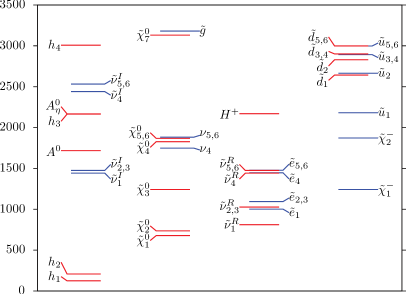
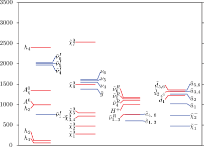
Figure 1: The mass spectra of BLV (left) and BLVI (right).

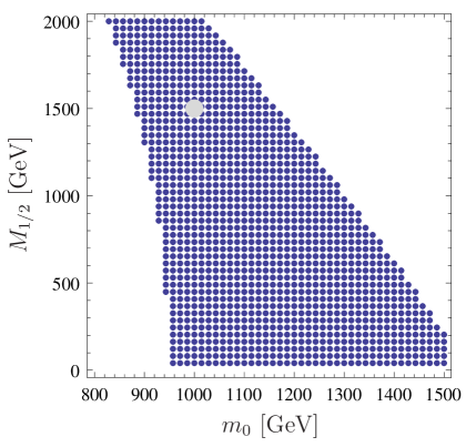
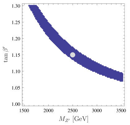
Figure 2: Allowed regions in the $m_{0}-M_{1/2}$ plane for $M_{Z^{\prime}}=2.5~{}\text{TeV},~{}\tan\beta^{\prime}=1.15$ (left) and in the $M_{Z^{\prime}}-\tan\beta^{\prime}$ plane for $m_{0}=1$ TeV and $M_{1/2}=1.5$ TeV (right). In both plots we have fixed in addition $\tan\beta=20$ and $A_{0}=-1.5$ TeV. The grey dot indicates the selected benchmark point (BLV).

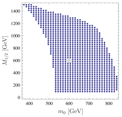
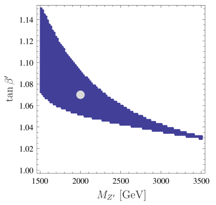
Figure 3: Allowed regions in the $m_{0}-M_{1/2}$ plane for $M_{Z^{\prime}}=2~{}\text{TeV},~{}\tan\beta^{\prime}=1.07$ (left) and in the $M_{Z^{\prime}}-\tan\beta^{\prime}$ plane for $m_{0}=0.6$ TeV and $M_{1/2}=0.6$ TeV (right). In both plots we have fixed in addition $\tan\beta=10$ and $A_{0}=0$. The grey dot indicates the selected benchmark point (BLVI).

In all numerical evaluations we have used the following SM input: $G_{F}=1.6639\cdot 10^{-5}$ GeV^-2, $m_{Z}=91.187$ GeV, $m_{\tau}=1.7771$ GeV, $m_{t}=172.9$ GeV, $m_{b}(m_{b})=4.2$ GeV and $\alpha_{s}(m_{Z})=0.119$. The latter two are $\overline{MS}$ values that are converted to the $\overline{DR}$ scheme. Moreover, we have fixed the neutrino Yukawa couplings such that the light neutrino masses can be explained. As this requires the maximum of $|Y_{\nu,ij}|$ to be at most $10^{-5}$, these couplings do not play any role in the considerations here. Because of their smallness, one can automatically satisfy the constraints from the nonobservation of rare decays such as $\mu\to e\gamma$ over all the parameter space. This is in contrast to the usual MSSM augmented by the various seesaw mechanisms, as discussed in e.g. Esteves:2009vg ; Esteves:2010ff and references therein.

As a starting point for our numerical investigations, we have taken the two points defined in Table 2. In analogy to Ref. O'Leary:2011yq , we label them BLV and BLVI (see Fig. 1). BLVI has a spectrum close to the existing LHC exclusion bounds. Note, however, that the high-scale input corresponds to different SUSY particle masses in comparison to the CMSSM because the running of the parameters is not the same and also the mass matrices differ. In contrast, BLV has quite a heavy spectrum and can only be discovered at $\sqrt{s}=14$ TeV. As discussed above, in this model the extra gauge group implies additional D terms to the sfermion masses. The requirement that the mass-squared parameters for all the sfermions are positive restricts the allowed range for $\tan\beta^{\prime}$, as can be seen in Figs. 2 and 3. This is a consequence of the large mass for the $Z^{\prime}$. Clearly this restriction is more severe for large $M_{Z^{\prime}}$ and less severe for large values of $m_{0}$ and $M_{1/2}$.

For completeness, we note that these points would give too large a relic density, which however is not an insurmountable problem and can easily be fixed without changing the collider phenomenology. In case of BLV one would need to invoke nonuniversal boundary conditions for the bileptons to change its mass. In this way one obtains an efficient annihilation of the lightest neutralino via a bilepton resonance as discussed in Basso:2012gz but having at the same time only tiny effects on the various decay branching ratios. In case of the BLVI the addition of a nonthermally produced gravitino with a mass of 10 GeV gives the correct relic density yielding a lifetime for the neutralino of about $10^{-3}$ seconds. This is sufficiently long-lived to appear as a stable particle at the LHC and at the same time sufficiently short-lived so that there are no problems with big bang nucleosynthesis.

III.3 $Z^{\prime}$ phenomenology

The mass of additional vector bosons as well as their mixing with the SM $Z$ boson, which implies, for example, a deviation of the fermion couplings to the $Z$ boson compared to SM expectations, is severely constrained by precision measurements from the LEP experiments Alcaraz:2006mx ; Erler:2009jh ; Nakamura:2010zzi . The bounds are on both the mass of the $Z^{\prime}$ and the mixing with the standard model $Z$ boson, where the latter is constrained by $|\sin(\Theta_{W^{\prime}})<0.0002|$. Using Eq. (34) together with Eq. (37) as well as the values of the running gauge couplings, a limit on the $Z^{\prime}$ mass of about 1.2 TeV is obtained. Taking in addition the bounds obtained from $U$, $T$ and $S$ parameters into account Cacciapaglia:2006pk one gets $M_{Z^{\prime}}/(Q_{e}^{B-L}{g_{BL}})>6.7$ TeV that for ${g_{BL}}\simeq 0.55$ would imply $M_{Z^{\prime}}\raise 1.29167pt\hbox{$\;>$\kern-7.5pt\raise-4.73611pt\hbox{$\sim\;$}}1.84$ TeV. However, this coupling has to be replaced by the effective coupling that gets modified due to gauge kinetic mixing: see Appendix A. Therefore, the above formula reads in our model $M_{Z^{\prime}}/(Q_{e}^{B-L}({g_{BL}}+{\bar{g}}))>6.7$ TeV, and ${g_{BL}}\simeq 0.55,{\bar{g}}\simeq-0.11$ imply $M_{Z^{\prime}}\raise 1.29167pt\hbox{$\;>$\kern-7.5pt\raise-4.73611pt\hbox{$\sim\;$}}1.47$ TeV.

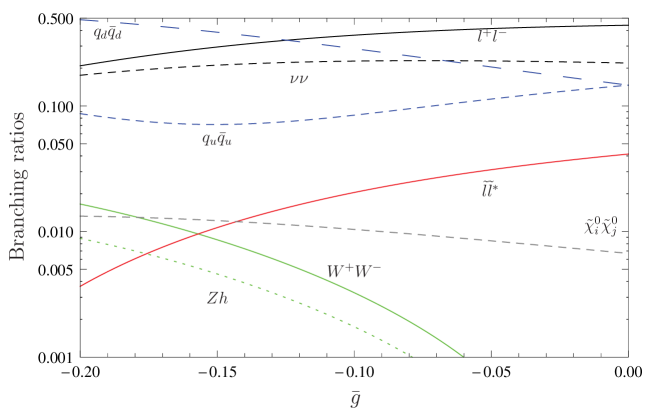
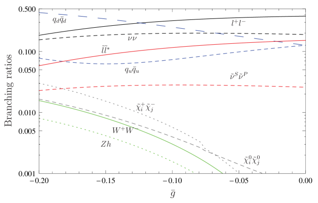
Figure 4: Branching ratios of the $Z^{\prime}$ at the considered parameter points BLV (above) and BLVI (below) as a function of the off-diagonal coupling parameter $\bar{g}$.

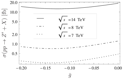
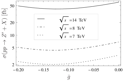
Figure 5: LHC production cross sections of the $Z^{\prime}$ at the considered parameter points BLV (left) and BLVI (right) and three different center-of-mass energies as a function of the off-diagonal coupling parameter $\bar{g}$.

The $Z^{\prime}$ dominantly decays into SM fermions as can be seen in Fig. 4 where we show the branching ratios as a function of $\bar{g}$. We have fixed all other parameters as given for the two study points in Table 2. For the study points themselves we find ${\bar{g}}\simeq-0.11$, which has to be compared with ${g_{BL}}\simeq 0.55$. As they are of the same order of magnitude, one can easily understand the strong dependence of the various branching ratios after inspecting the couplings given in Appendix A.1. The $Z^{\prime}$ can also decay into supersymmetric particles Gherghetta:1996yr with branching ratios of up to $O(10\%)$ in our model. We find that, in particular, decays into charged sleptons can have a sizable branching ratio, as can also be seen in Fig. 4. Besides the decays, the cross sections also depend on gauge kinetic mixing as demonstrated in Fig. 5 where we show the $Z^{\prime}$ cross section for $\sqrt{s}=7,8$, and 14 TeV as a function of $\bar{g}$. For the PDFs we have used the set CTEQ6L1 cteq .

Parameter point	${\bar{g}}=-0.11$	${\bar{g}}=0$
BLV	1770 GeV	1965 GeV
BLVI	1730 GeV	1900 GeV

Table 3: Current bounds on $M_{Z^{\prime}}$ in the supersymmetric $B-L$ model derived from 5 fb^-1 of ATLAS data for both benchmark points using different assumptions as discussed in the text.

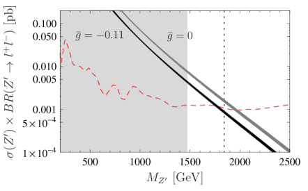
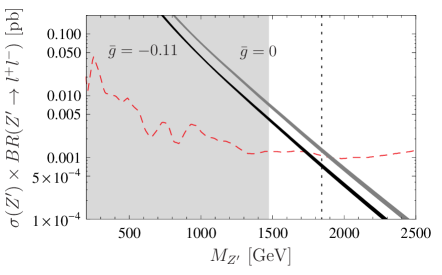
Figure 6: Current limits on $M_{Z^{\prime}}$ for combined lepton production for the study points BLV (left) and BLVI (right). The red dashed curve shows the recent experimental ATLAS limits Collaboration:2011dca . The black and grey bands are the dilepton production cross sections at the $Z^{\prime}$ peak for the case of $U(1)$ mixing (black) and without (grey). The grey shaded area shows the mass range forbidden by LEP II, while the black dotted line shows the LEP limits without taking into account gauge kinetic mixing.

Recently ATLAS and CMS Collaboration:2011dca ; Chatrchyan:2011wq have updated the results for $Z^{\prime}$ searches. As they do not give direct bounds for our model, we have calculated the corresponding signal cross section. If one took only final states containing SM particles into account and neglected gauge kinetic mixing, one would find a lower bound of $1970~{}\text{GeV}\leq M_{Z^{\prime}}$. Taking into account gauge kinetic mixing we find for ${\bar{g}}\simeq-0.1$ a bound of 1790 GeV. Moreover, for both our study points, final states containing supersymmetric particles are also present as discussed above. This leads to an increase of the width and thus to a reduction of the signal cross sections. Therefore the bounds are less severe, as has also been discussed in the context of related models Chang:2011be ; Corcella:2012dw . In contrast to previous studies, we encounter here a case where neglecting gauge kinetic effects would lead to a significantly incorrect bound. In fact the bound obtained at LHC differs by about 200 GeV depending on whether kinetic mixing is correctly taken into account or not, as can be seen from Table 3. This is further exemplified in Fig. 6 where we display the cross section into leptons (summed over electrons and muons) as a function of $M_{Z^{\prime}}$. The grey area is excluded by precision LEP data whereas the red dashed line gives the bound on the signal cross section as obtained by the ATLAS Collaboration Collaboration:2011dca . Note that the effect on the LEP limits is even stronger, as can be seen at the dotted line in Fig. 6. The CMS bounds are similar and thus lead to nearly the same limits. Clearly it would be desirable to have a combined analysis by both collaborations.

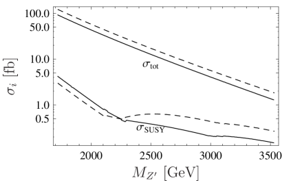
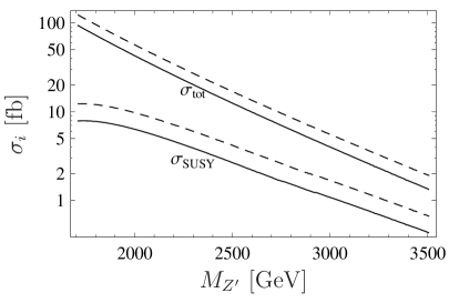
Figure 7: Cross sections for $pp\to Z^{\prime}$ at LHC with $\sqrt{s}=$14 TeV as a function of $M_{Z^{\prime}}$ for the benchmark points BLV (left) and BLVI (right). The upper two lines show the total cross section whereas the lower two show the cross section in SUSY particles via a $Z^{\prime}$. The solid lines give the cross section taking into account gauge kinetic mixing whereas the dashed ones give the cross section if gauge kinetic mixing were neglected.

In Fig. 7 we give the cross sections for $pp\to Z^{\prime}$ at LHC with $\sqrt{s}=$14 TeV as a function of $M_{Z^{\prime}}$ for the two benchmark points. To demonstrate the importance of gauge kinetic mixing, we display the values taking it into account (solid lines) and those where it is neglected (dashed lines). Comparing both data points, one sees that the dependence on the gauge kinetic mixing on the SUSY final states depends on the underlying soft SUSY-breaking parameters. For BLVI, the dominant SUSY channels always involve the sleptons and therefore kinetic mixing reduces the cross section. In contrast, for BLV and small values of $M_{Z^{\prime}}$, final states including two neutralinos with large bileptino contents are important. Therefore, the cross section is larger with kinetic mixing than without. However, the masses of these neutralinos rapidly increase with $M_{Z^{\prime}}$ and slepton production is the dominant SUSY channel for $M_{Z^{\prime}}>2.3$ TeV.

III.4 Slepton production via $Z^{\prime}$ as discovery channel

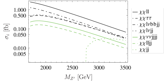
Figure 8: Cross sections for the dominant final states resulting from the SUSY particles that are produced via a $Z^{\prime}$ for benchmark point BLVI. The symbols correspond to $\chi\mathrel{\widehat{=}}\tilde{\chi}^{0}_{1}$, l $\mathrel{\widehat{=}}$ (anti)lepton ($e,\mu$), b $\mathrel{\widehat{=}}$ (anti)bottom quark, $\nu\mathrel{\widehat{=}}$ neutrino, j $\mathrel{\widehat{=}}$ jet resulting from a quark of the first two generations.

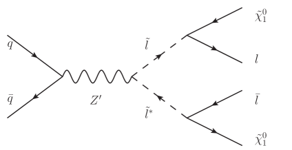
Figure 9: Feynman diagram for the production of $\tilde{l}\tilde{l}^{*}$ via an $s$-channel $Z^{\prime}$exchange and the subsequent decay into $l^{+}l^{-}\tilde{\chi}^{0}_{1}\tilde{\chi}^{0}_{1}$.

A heavy $Z^{\prime}$ allows the production of electroweak SUSY particles with masses of several hundred GeV implying that this might be an important discovery channel as has also been discussed in related models Kang:2004bz ; Chang:2011be ; Corcella:2012dw ; Baumgart:2006pa . In contrast to the previous studies, gauge kinetic mixing is important as we have seen above. In the following we will first take benchmark point BLVI to discuss some basic features. Much as in the MSSM, the $R$ sleptons decay almost always into a lepton and the lightest neutralino, whereas the $L$ sleptons decay dominantly into the lighter chargino and a neutrino, or the second lightest neutralino and a lepton, in roughly the ratio two to one. The lighter chargino and the second lightest neutralino, which have a large wino fraction, decay dominantly into the lightest neutralino and a vector boson. The neutralino decay can also result in a final-state Higgs boson. Therefore one has additional leptons and jets stemming from the decays of the vector boson and Higgs bosons.

In Fig. 8 we display the most important final states resulting from the cascade decays of supersymmetric particles originating from the $Z^{\prime}$. We have fixed the soft SUSY-breaking parameters as in BLVI. Nevertheless, the masses change as a function of $M_{Z^{\prime}}$ as the corresponding bilepton vevs enter the mass matrices, see e.g. Secs. II.5 and II.6. The dominant final state contains two leptons and two lightest supersymmetric particles stemming from slepton production as displayed in Fig. 9. For these points, sleptons are hardly ever produced in the cascade decays of squarks and gluinos, in contrast to the neutralinos and charginos.

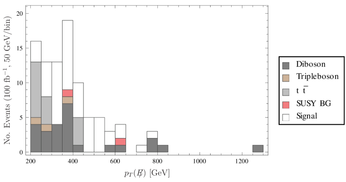
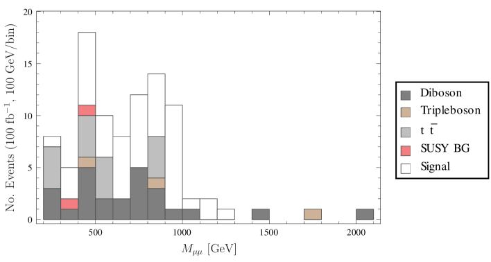
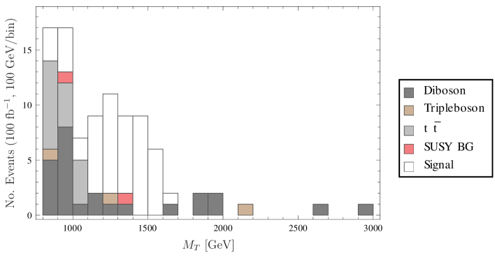
Figure 10: Histograms of the $\mu^{+}\mu^{-}+E\!\!\!/$ production with the applied cuts $M_{\mu\mu}>200$ GeV, $p_{T}(E\!\!\!/)>200$ GeV and $M_{T}>800$ GeV as a function of the missing energy, muon pair invariant mass and the transverse cluster mass.

For this reason the $Z^{\prime}$ decays are a potential discovery channel for sleptons. We have performed a basic Monte Carlo study using WHIZARD Kilian:2007gr to generate the signal in the case of smuon pair production and simulated the background. For the background, we considered diboson production, triple vector boson production and $t\bar{t}$ production as well as neutralino and chargino production including both direct production via Drell-Yan processes and cascade decays from squarks and gluinos. However, the contributions from the latter are rather small. We have applied the following cuts to suppress the background

• Invariant mass of the muon pair: $M_{\mu\mu}>200$ GeV.

• Missing transverse momentum: $p_{T}(E\!\!\!/)>200$ GeV.

• A cut on the transverse cluster mass

  $$M_{T}=\sqrt{\left(\sqrt{p_{T}^{2}(\mu^{+}\mu^{-})+M_{\mu\mu}^{2}}+p_{T}(E\!\!\!/)\right)^{2}-\left(\vec{p}_{T}(\mu^{+}\mu^{-})+\vec{p}_{T}(E\!\!\!/)\right)^{2}}$$ (58)

  with $\vec{p}_{T}$ being the 2D vector of the transverse momentum and $\vec{p}_{T}(\mu^{+}\mu^{-})=\vec{p}_{T}(\mu^{+})+\vec{p}_{T}(\mu^{-})$. We required $M_{T}>800$ GeV.

• For the suppression of $t\bar{t}$ and squark/gluino cascade decays, we set a cut on the transverse momentum of the hardest jet: $p_{T,jet}<40$ GeV.

In Fig. 10 we display the resulting distributions for an integrated luminosity of 100 fb^-1 at $\sqrt{s}=14$ TeV. The resulting significance, which is calculated as

$$s=\frac{N_{\text{Signal}}}{\sqrt{N_{\text{BG}}}}\,,$$ (59)

is 7.5 $\sigma$, which is sufficient to claim discovery for this example.

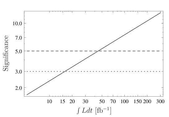
Figure 11: Evolution of the significance level with growing integrated luminosity. The discussed significance at 100 fb^-1 fixes the curve. The borders for 3 and 5$\sigma$ are shown as dotted and dashed lines.

As can be seen from Fig. 11, with a luminosity of about 45 fb^-1 one crosses the $5\sigma$ level. These numbers have been obtained using tree-level calculations and it is known that higher-order corrections are important in this context, see e.g. Fuks:2007gk and references therein. In case of nonsupersymmetric models one obtains K-factors of about 1.2-1.4 depending on the details of the models Fuks:2007gk ; Accomando:2010fz . However, as it is not obvious how corrections due to supersymmetric particles will change this or how they affect the background reactions, we will stick to tree-level calculations here.

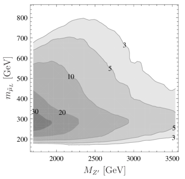
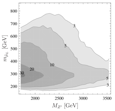
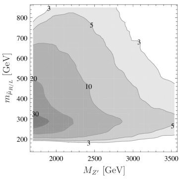
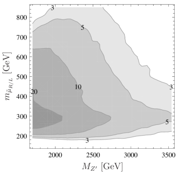
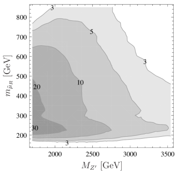
Figure 12: Significance level of the smuon discovery as a function of the respective lightest $\tilde{\mu}$ mass and $M_{Z^{\prime}}$ for ${\cal L}=100$ fb^-1 and $m_{{\tilde{\chi}}^{0}_{1}}=140$ GeV. Left column: looser cuts [$p_{T}(E\!\!\!/)>200$ GeV, $M_{\mu\mu}>200$ GeV, $M_{T}>800$ GeV]. Right column: tighter cuts [$p_{T}(E\!\!\!/)>250$ GeV, $M_{\mu\mu}>300$ GeV]. The smuon mass relations are (first row) $m_{\tilde{\mu}_{R}}=1.2\,m_{\tilde{\mu}_{L}}$, (second row) $m_{\tilde{\mu}_{R}}=m_{\tilde{\mu}_{L}}$ and (last row) $m_{\tilde{\mu}_{L}}=1.2\,m_{\tilde{\mu}_{R}}$.

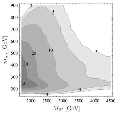
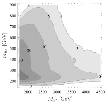
Figure 13: Significance level of the smuon discovery for ${\cal L}=300$ fb^-1, $m_{{\tilde{\chi}}^{0}_{1}}=140$ GeV $m_{\tilde{\mu}_{L}}=1.2\,m_{\tilde{\mu}_{R}}$. Left: looser cuts [$p_{T}(E\!\!\!/)>200$ GeV, $M_{\mu\mu}>200$ GeV, $M_{T}>800$ GeV]. Right: tighter cuts [$p_{T}(E\!\!\!/)>250$ GeV, $M_{\mu\mu}>300$ GeV]. The mass of the lightest supersymmetric particle is $140$ GeV.

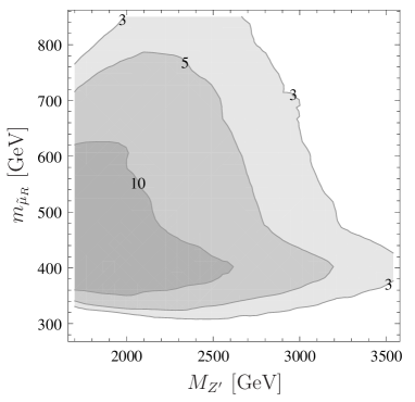
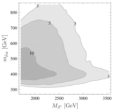
Figure 14: Significance level of the smuon production for ${\cal L}=100$ fb^-1, $m_{{\tilde{\chi}}^{0}_{1}}=280$ GeV $m_{\tilde{\mu}_{L}}=1.2\,m_{\tilde{\mu}_{R}}$. Left: looser cuts [$p_{T}(E\!\!\!/)>200$ GeV, $M_{\mu\mu}>200$ GeV, $M_{T}>800$ GeV]. Right: tighter cuts [$p_{T}(E\!\!\!/)>250$ GeV, $M_{\mu\mu}>300$ GeV].

The results depend so far mainly on the following quantities: $M_{Z^{\prime}}$, $m_{\tilde{l}}$, $m_{\tilde{\chi}^{0}_{i}}$ and $m_{\tilde{\chi}^{+}_{j}}$ and on the nature of the neutralinos and charginos. We assume in the following that the lightest two neutralinos and the lighter chargino are mainly the MSSM gauginos as in our study points. However, we will depart to some extent from the GUT assumptions: we will fix the masses of squarks and gluinos to the values they take in benchmark point BLVI in Table 2 but vary the slepton masses freely. As we are interested in relatively light sleptons with masses down to 200 GeV we fix $m_{\tilde{\chi}^{0}_{1}}=140$ GeV and $m_{\tilde{\chi}^{0}_{2}}=m_{\tilde{\chi}^{+}_{1}}=2\,m_{\tilde{\chi}^{0}_{1}}$. We have performed a scan over slepton masses and $M_{Z^{\prime}}$ fixing the ratio of the masses for $R$ sleptons to $L$ sleptons to 1.2, 1, and 1/1.2. The different ratios can in principle be obtained by varying $\tan\beta^{\prime}$, as can also be seen from the formulas in Sec. II.6. We have also investigated the effect of tightening the previous cuts to $p_{T}(E\!\!\!/)>250~{}\text{GeV}$ and $M_{\mu\mu}>300~{}\text{GeV}$. In Fig. 12 we show our results for the significance assuming an integrated luminosity of 100 fb^-1. We find a significant dependence on the ratio of the smuon masses which is due to the fact that we consider here only smuon decays into $\mu\tilde{\chi}^{0}_{1}$. This is also the reason for the “promontory” for slepton masses up to 300 GeV as there both $L$ and $R$ smuons can decay only into this final state. The regions should even become somewhat larger if one includes also the smuon decays into $\mu\tilde{\chi}^{0}_{2}$ and $\nu\tilde{\chi}^{-}_{1}$. However, one has then to consider the background of squark and gluino cascade decays that depend on the details of the parameter point under study.

In Fig. 13 we display the same for the case of $m_{\tilde{\mu}_{L}}=1.2\,m_{\tilde{\mu}_{R}}$ but taking a luminosity of 300 fb^-1. As expected, the reach increases for both $m_{\tilde{\mu}}$ and $M_{Z^{\prime}}$. For the other two ratios of slepton masses we find the same behavior. In Fig. 14 we show the changes for increased neutralino and chargino masses $m_{\tilde{\chi}^{0}_{1}}=280$ GeV and ${\tilde{\chi}^{0}_{2}}={\tilde{\chi}^{+}_{1}}=475~{}$GeV, which are the values obtained in the constrained model at BLVI. As expected, the 5$\sigma$ significance is restricted to larger values of the smuon mass as the leptons are softer than in the previous example.

IV Conclusion

We have studied a supersymmetric model where the gauge group is extended by an additional $U(1)_{B-L}$ factor resulting in a $Z^{\prime}$ with a mass in the TeV range. Such models can emerge as effective models from heterotic string models. An important feature of this class of models is gauge kinetic mixing. Here we focused on its impact for the phenomenology of the extra vector boson. We have first shown that bounds on its mass due to collider searches get significantly reduced once the gauge kinetic mixing is taken into account: LEP bounds by about 400 GeV and LHC bounds by about 200 GeV. Moreover, this implies that now LHC bounds are more important than the ones originating from LEP data. Second we have shown that these bounds get further reduced if the $Z^{\prime}$ can decay into supersymmetric particles. In our model the most important decays are into sleptons, neutralinos and charginos.

Moreover, we have discussed the reach of LHC with $\sqrt{s}=14$ TeV for the discovery of smuons, which is an important possibility should squark or gluino cascades in sufficient quantities be inaccessible. For an integrated luminosity of 100 fb^-1 (300 fb^-1) we have found that sleptons with masses of up to 800 GeV (900 GeV) can be discovered this way, provided the $Z^{\prime}$ is lighter than about 2.8 TeV (3.1 TeV). This result depends only mildly on the nature of the smuons provided that their decays into muons are not suppressed. Apart from detector effects, similar results hold for selectrons. Staus, on the other hand, require a detailed study and we expect a reduced reach at the LHC due to the hadronic decays of the resulting $\tau$ leptons.

Appendix A $Z^{\prime}$ couplings

In this section we collect the formulas for the couplings of $Z^{\prime}$ to the fermions and scalars in this model.

A.1 Couplings to fermions

The couplings given below follow from the terms in the Lagrangian

$$\bar{f_{i}}\gamma^{\mu}(c_{Lf,ij}P_{L}+c_{Rf,ij}P_{R})f_{j}Z^{\prime}_{\mu}\,.$$ (60)

• Charged leptons: $Z^{\prime}-\bar{e}_{i}-e_{j}$

  $$c_{Le,ij}= \frac{1}{2}\delta_{ij}\Big{(}\Big{(}g_{1}\sin\Theta_{W}-g_{2}\cos\Theta_{W}\Big{)}\sin{\Theta^{\prime}}_{W}+\Big{(}{\bar{g}}+{g_{BL}}\Big{)}\cos{\Theta^{\prime}}_{W}\Big{)}\,,$$ (61)

  $$c_{Re,ij}= \,\frac{1}{2}\delta_{ij}\Big{(}2g_{1}\sin\Theta_{W}\sin{\Theta^{\prime}}_{W}+\Big{(}2{\bar{g}}+{g_{BL}}\Big{)}\cos{\Theta^{\prime}}_{W}\Big{)}\,.$$ (62)

• Neutrinos: $Z^{\prime}-\nu_{i}-\nu_{j}$

  $$c_{L\nu,ij}= \frac{1}{2}\Big{(}\Big{(}\Big{(}g_{1}\sin\Theta_{W}+g_{2}\cos\Theta_{W}\Big{)}\sin{\Theta^{\prime}}_{W}+\Big{(}{\bar{g}}+{g_{BL}}\Big{)}\cos{\Theta^{\prime}}_{W}\Big{)}\sum_{a=1}^{3}U^{V,*}_{ja}U_{{ia}}^{V}$$

  $$-{g_{BL}}\cos{\Theta^{\prime}}_{W}\sum_{a=1}^{3}U^{V,*}_{j3+a}U_{{i3+a}}^{V}\Big{)}\,,$$ (63)

  $$c_{R\nu,ij}= \,-\frac{1}{2}\Big{(}\Big{(}\Big{(}g_{1}\sin\Theta_{W}+g_{2}\cos\Theta_{W}\Big{)}\sin{\Theta^{\prime}}_{W}+\Big{(}{\bar{g}}+{g_{BL}}\Big{)}\cos{\Theta^{\prime}}_{W}\Big{)}\sum_{a=1}^{3}U^{V,*}_{ia}U_{{ja}}^{V}$$

  $$-{g_{BL}}\cos{\Theta^{\prime}}_{W}\sum_{a=1}^{3}U^{V,*}_{i3+a}U_{{j3+a}}^{V}\Big{)}\,.$$ (64)

  $U^{V}_{kl}$ is the unitary $6\times 6$ matrix that diagonalizes the neutrino mass matrix.

• Up-type quarks: $Z^{\prime}-\bar{u}_{i\alpha}-u_{j\beta}$

  $$c_{Lu,ij}= -\frac{1}{6}\delta_{\alpha\beta}\delta_{ij}\Big{(}\Big{(}-3g_{2}\cos\Theta_{W}+g_{1}\sin\Theta_{W}\Big{)}\sin{\Theta^{\prime}}_{W}+\Big{(}{\bar{g}}+{g_{BL}}\Big{)}\cos{\Theta^{\prime}}_{W}\Big{)}\,,$$ (65)

  $$c_{Ru,ij}= \,-\frac{1}{6}\delta_{\alpha\beta}\delta_{ij}\Big{(}4g_{1}\sin\Theta_{W}\sin{\Theta^{\prime}}_{W}+\Big{(}4{\bar{g}}+{g_{BL}}\Big{)}\cos{\Theta^{\prime}}_{W}\Big{)}\,.$$ (66)

• Down-type quarks: $Z^{\prime}-\bar{d}_{i\alpha}-d_{j\beta}$

  $$c_{Ld,ij}= -\frac{1}{6}\delta_{\alpha\beta}\delta_{ij}\Big{(}\Big{(}3g_{2}\cos\Theta_{W}+g_{1}\sin\Theta_{W}\Big{)}\sin{\Theta^{\prime}}_{W}+\Big{(}{\bar{g}}+{g_{BL}}\Big{)}\cos{\Theta^{\prime}}_{W}\Big{)}\,,$$ (67)

  $$c_{Rd,ij}= \,\frac{1}{6}\delta_{\alpha\beta}\delta_{ij}\Big{(}2g_{1}\sin\Theta_{W}\sin{\Theta^{\prime}}_{W}+\Big{(}2{\bar{g}}-{g_{BL}}\Big{)}\cos{\Theta^{\prime}}_{W}\Big{)}\,.$$ (68)

• Neutralinos: $Z^{\prime}-\tilde{\chi}^{0}_{i}-\tilde{\chi}^{0}_{j}$

  $$c_{L\tilde{\chi}^{0},ij}= \frac{1}{2}\Big{(}N^{*}_{j3}\Big{(}\Big{(}g_{1}\sin\Theta_{W}+g_{2}\cos\Theta_{W}\Big{)}\sin{\Theta^{\prime}}_{W}+{\bar{g}}\cos{\Theta^{\prime}}_{W}\Big{)}N_{{i3}}$$

  $$-N^{*}_{j4}\Big{(}g_{1}\sin\Theta_{W}\sin{\Theta^{\prime}}_{W}+g_{2}\cos\Theta_{W}\sin{\Theta^{\prime}}_{W}+{\bar{g}}\cos{\Theta^{\prime}}_{W}\Big{)}N_{{i4}}$$

  $$+2{g_{BL}}\cos{\Theta^{\prime}}_{W}\Big{(}N^{*}_{j6}N_{{i6}}-N^{*}_{j7}N_{{i7}}\Big{)}\Big{)}\,,$$ (69)

  $$c_{R\tilde{\chi}^{0},ij}= \,-\frac{1}{2}\Big{(}N^{*}_{i3}\Big{(}\Big{(}g_{1}\sin\Theta_{W}+g_{2}\cos\Theta_{W}\Big{)}\sin{\Theta^{\prime}}_{W}+{\bar{g}}\cos{\Theta^{\prime}}_{W}\Big{)}N_{{j3}}$$

  $$-N^{*}_{i4}\Big{(}g_{1}\sin\Theta_{W}\sin{\Theta^{\prime}}_{W}+g_{2}\cos\Theta_{W}\sin{\Theta^{\prime}}_{W}+{\bar{g}}\cos{\Theta^{\prime}}_{W}\Big{)}N_{{j4}}$$

  $$+2{g_{BL}}\cos{\Theta^{\prime}}_{W}\Big{(}N^{*}_{i6}N_{{j6}}-N^{*}_{i7}N_{{j7}}\Big{)}\Big{)}\,.$$ (70)

  $N_{kl}$ is the unitary $7\times 7$ matrix that diagonalizes the neutralino mass matrix.

• Charginos: $Z^{\prime}-\tilde{\chi}^{+}_{i}-\tilde{\chi}^{-}_{j}$

  $$c_{L\tilde{\chi}^{\pm},ij}= \,-\frac{1}{2}\Big{(}2g_{2}U^{*}_{j1}\cos\Theta_{W}\sin{\Theta^{\prime}}_{W}U_{{i1}}$$

  $$-U^{*}_{j2}\Big{(}\Big{(}g_{1}\sin\Theta_{W}-g_{2}\cos\Theta_{W}\Big{)}\sin{\Theta^{\prime}}_{W}+{\bar{g}}\cos{\Theta^{\prime}}_{W}\Big{)}U_{{i2}}\Big{)}\,,$$ (71)

  $$c_{R\tilde{\chi}^{\pm},ij}= \,-\frac{1}{2}\Big{(}2g_{2}V^{*}_{i1}\cos\Theta_{W}\sin{\Theta^{\prime}}_{W}V_{{j1}}$$

  $$-V^{*}_{i2}\Big{(}\Big{(}g_{1}\sin\Theta_{W}-g_{2}\cos\Theta_{W}\Big{)}\sin{\Theta^{\prime}}_{W}+{\bar{g}}\cos{\Theta^{\prime}}_{W}\Big{)}V_{{j2}}\Big{)}\,.$$ (72)

  $U_{kl}$ and $V_{kl}$ are the unitary $2\times 2$ matrices needed to diagonalize chargino mass matrix.

A.2 Couplings to scalars

The couplings given below follow from the terms in the Lagrangian

$$c_{s,ij}\tilde{s}_{i}\tilde{s}_{j}^{*}\left(p_{s_{i}}^{\mu}-p_{s^{*}_{j}}^{\mu}\right)Z^{\prime}_{\mu}\,,$$ (73)

where $p_{s_{i}}$ and $p_{s^{*}_{j}}$ are the four-momenta of the scalars. In the following, $Z^{p}_{kl}$ denote the matrices needed to diagonalize the respective underlying mass matrix of the particles $p$.

• Charged sleptons: $Z^{\prime}-\tilde{e}_{i}-\tilde{e}_{j}^{*}$

  $$c_{e,ij}= \frac{1}{2}\Big{(}\Big{(}\Big{(}g_{1}\sin\Theta_{W}-g_{2}\cos\Theta_{W}\Big{)}\sin{\Theta^{\prime}}_{W}+\Big{(}{\bar{g}}+{g_{BL}}\Big{)}\cos{\Theta^{\prime}}_{W}\Big{)}\sum_{a=1}^{3}Z^{E,*}_{ia}Z_{{ja}}^{E}$$

  $$+\Big{(}2g_{1}\sin\Theta_{W}\sin{\Theta^{\prime}}_{W}+\Big{(}2{\bar{g}}+{g_{BL}}\Big{)}\cos{\Theta^{\prime}}_{W}\Big{)}\sum_{a=1}^{3}Z^{E,*}_{i3+a}Z_{{j3+a}}^{E}\Big{)}\,.$$ (74)

• Sneutrinos: $Z^{\prime}-\tilde{\nu}^{P}_{i}-\tilde{\nu}_{j}^{S*}$

  $$c_{\nu,ij}= \frac{i}{2}\Big{(}-\Big{(}\Big{(}g_{1}\sin\Theta_{W}+g_{2}\cos\Theta_{W}\Big{)}\sin{\Theta^{\prime}}_{W}+\Big{(}{\bar{g}}+{g_{BL}}\Big{)}\cos{\Theta^{\prime}}_{W}\Big{)}\sum_{a=1}^{3}Z^{P,*}_{ia}Z^{S,*}_{ja}$$

  $$-{g_{BL}}\cos{\Theta^{\prime}}_{W}\sum_{a=1}^{3}Z^{P,*}_{i3+a}Z^{S,*}_{j3+a}\Big{)}\,.$$ (75)

• Up-type squarks: $Z^{\prime}-\tilde{u}_{i\alpha}-\tilde{u}_{j\beta}^{*}$

  $$c_{q_{u},ij}= -\frac{1}{6}\delta_{\alpha\beta}\Big{(}\Big{(}\Big{(}-3g_{2}\cos\Theta_{W}+g_{1}\sin\Theta_{W}\Big{)}\sin{\Theta^{\prime}}_{W}+\Big{(}{\bar{g}}+{g_{BL}}\Big{)}\cos{\Theta^{\prime}}_{W}\Big{)}\sum_{a=1}^{3}Z^{U,*}_{ia}Z_{{ja}}^{U}$$

  $$+\Big{(}4g_{1}\sin\Theta_{W}\sin{\Theta^{\prime}}_{W}+\Big{(}4{\bar{g}}+{g_{BL}}\Big{)}\cos{\Theta^{\prime}}_{W}\Big{)}\sum_{a=1}^{3}Z^{U,*}_{i3+a}Z_{{j3+a}}^{U}\Big{)}\,.$$ (76)

• Down-type squarks: $Z^{\prime}-\tilde{d}_{i\alpha}-\tilde{d}_{j\beta}^{*}$

  $$c_{q_{d},ij}= -\frac{1}{6}\delta_{\alpha\beta}\Big{(}\Big{(}\Big{(}3g_{2}\cos\Theta_{W}+g_{1}\sin\Theta_{W}\Big{)}\sin{\Theta^{\prime}}_{W}+\Big{(}{\bar{g}}+{g_{BL}}\Big{)}\cos{\Theta^{\prime}}_{W}\Big{)}\sum_{a=1}^{3}Z^{D,*}_{ia}Z_{{ja}}^{D}$$

  $$+\Big{(}-2g_{1}\sin\Theta_{W}\sin{\Theta^{\prime}}_{W}+\Big{(}-2{\bar{g}}+{g_{BL}}\Big{)}\cos{\Theta^{\prime}}_{W}\Big{)}\sum_{a=1}^{3}Z^{D,*}_{i3+a}Z_{{j3+a}}^{D}\Big{)}\,.$$ (77)

• Charged Higgs: $Z^{\prime}-H^{-}_{i}-H^{+}_{j}$

  $$c_{H^{\pm},ij}= \frac{1}{2}\delta_{ij}\Big{(}\Big{(}g_{1}\sin\Theta_{W}-g_{2}\cos\Theta_{W}\Big{)}\sin{\Theta^{\prime}}_{W}+{\bar{g}}\cos{\Theta^{\prime}}_{W}\Big{)}\,.$$ (78)

• $CP$-odd and $CP$-even Higgs: $Z^{\prime}-A^{0}_{i}-h_{j}$

  $$c_{Ah,ij}= \frac{i}{2}\Big{(}-\Big{(}\Big{(}g_{1}\sin\Theta_{W}+g_{2}\cos\Theta_{W}\Big{)}\sin{\Theta^{\prime}}_{W}+{\bar{g}}\cos{\Theta^{\prime}}_{W}\Big{)}Z_{{i1}}^{A}Z_{{j1}}^{H}$$

  $$+\Big{(}\Big{(}g_{1}\sin\Theta_{W}+g_{2}\cos\Theta_{W}\Big{)}\sin{\Theta^{\prime}}_{W}+{\bar{g}}\cos{\Theta^{\prime}}_{W}\Big{)}Z_{{i2}}^{A}Z_{{j2}}^{H}$$

  $$-2{g_{BL}}\cos{\Theta^{\prime}}_{W}\Big{(}Z_{{i3}}^{A}Z_{{j3}}^{H}-Z_{{i4}}^{A}Z_{{j4}}^{H}\Big{)}\Big{)}\,.$$ (79)

A.3 Coupling to vector bosons

The only three-vector-boson vertex containing a $Z^{\prime}$ is the coupling $Z^{\prime}_{\mu}-W^{+}_{\rho}-W^{-}_{\sigma}$. It is parametrized as follows:

$$c_{V_{i}V_{j}}\Big{(}g_{\rho\mu}\Big{(}-p^{{Z^{\prime}}_{{\mu}}}_{\sigma}+p^{W^{+}_{{\rho}}}_{\sigma}\Big{)}+g_{\rho\sigma}\Big{(}-p^{W^{+}_{{\rho}}}_{\mu}+p^{W^{-}_{{\sigma}}}_{\mu}\Big{)}+g_{\sigma\mu}\Big{(}-p^{W^{-}_{{\sigma}}}_{\rho}+p^{{Z^{\prime}}_{{\mu}}}_{\rho}\Big{)}\Big{)}Z^{\prime\mu}V_{i}^{\rho}V_{j}^{\sigma}\,,$$ (80)

with

$$c_{WW}=g_{2}\cos\Theta_{W}\sin{\Theta^{\prime}}_{W}\,.$$ (81)

A.4 Coupling to one vector boson and one scalar

The vertices are parametrized as follows:

$$c_{Vs,i}s_{i}g_{\sigma\mu}Z^{\prime\mu}V^{\sigma}\,.$$ (82)

• $Z$ and Higgs: $Z^{\prime}_{\mu}-Z_{\sigma}-h_{i}$

  $$c_{Zh,i} =\frac{1}{2}\Big{(}-v_{d}\Big{(}g_{1}{\bar{g}}\cos{\Theta^{\prime}}_{W}^{2}\sin\Theta_{W}+g_{2}^{2}\cos\Theta_{W}^{2}\cos{\Theta^{\prime}}_{W}\sin{\Theta^{\prime}}_{W}$$

  $$+\cos{\Theta^{\prime}}_{W}\Big{(}g_{1}^{2}\sin\Theta_{W}^{2}-{\bar{g}}^{2}\Big{)}\sin{\Theta^{\prime}}_{W}-g_{1}{\bar{g}}\sin\Theta_{W}\sin{\Theta^{\prime}}_{W}^{2}$$

  $$+g_{2}\cos\Theta_{W}\Big{(}g_{1}\sin\Theta_{W}\sin 2{\Theta^{\prime}}_{W}+{\bar{g}}\cos{\Theta^{\prime}}_{W}^{2}-{\bar{g}}\sin{\Theta^{\prime}}_{W}^{2}\Big{)}\Big{)}Z_{{i1}}^{H}$$

  $$-v_{u}\Big{(}g_{1}{\bar{g}}\cos{\Theta^{\prime}}_{W}^{2}\sin\Theta_{W}+g_{2}^{2}\cos\Theta_{W}^{2}\cos{\Theta^{\prime}}_{W}\sin{\Theta^{\prime}}_{W}$$

  $$+\cos{\Theta^{\prime}}_{W}\Big{(}g_{1}^{2}\sin\Theta_{W}^{2}-{\bar{g}}^{2}\Big{)}\sin{\Theta^{\prime}}_{W}-g_{1}{\bar{g}}\sin\Theta_{W}\sin{\Theta^{\prime}}_{W}^{2}$$

  $$+g_{2}\cos\Theta_{W}\Big{(}g_{1}\sin\Theta_{W}\sin 2{\Theta^{\prime}}_{W}+{\bar{g}}\cos{\Theta^{\prime}}_{W}^{2}-{\bar{g}}\sin{\Theta^{\prime}}_{W}^{2}\Big{)}\Big{)}Z_{{i2}}^{H}$$

  $$+2{g_{BL}}\sin 2{\Theta^{\prime}}_{W}\Big{(}v_{\eta}Z_{{i3}}^{H}+v_{\bar{\eta}}Z_{{i4}}^{H}\Big{)}\Big{)}\,.$$ (83)

References

- (1) H. P. Nilles, Phys.Rept. 110, 1 (1984).
- (2) M. Drees, R. Godbole, and P. Roy Theory and Phenomenology of Sparticles: An Account of Four-Dimensional N=1 Supersymmetry in High Energy Physics (World Scientific, Singapore, 2004).
- (3) B.C. Allanach, Phys.Rev. D83, 095019 (2011), arXiv:1102.3149.
- (4) O. Buchmueller et al., Eur.Phys.J. C71, 1634 (2011), arXiv:1102.4585.
- (5) B. Allanach, T. Khoo, C. Lester, and S. Williams, JHEP 1106, 035 (2011), arXiv:1103.0969.
- (6) G. Bertone et al., JCAP 1201, 015 (2012), arXiv:1107.1715.
- (7) O. Buchmueller et al., Eur.Phys.J. C71, 1722 (2011), arXiv:1106.2529.
- (8) O. Buchmueller et al., Eur.Phys.J. C72, 1878 (2012), arXiv:1110.3568.
- (9) C. Beskidt, W. de Boer, D. Kazakov, and F. Ratnikov, JHEP 1205, 094 (2012), arXiv:1202.3366.
- (10) L. Roszkowski, E. M. Sessolo, and Y.-L. S. Tsai, (2012), arXiv:1202.1503.
- (11) P. Bechtle et al., JHEP 1206, 098 (2012), arXiv:1204.4199.
- (12) ATLAS Collaboration, G. Aad et al., Phys.Lett. B710, 49 (2012), arXiv:1202.1408.
- (13) CMS Collaboration, S. Chatrchyan et al., Phys.Lett. B710, 26 (2012), arXiv:1202.1488.
- (14) C. F. Berger, J. S. Gainer, J. L. Hewett, and T. G. Rizzo, JHEP 0902, 023 (2009), arXiv:0812.0980.
- (15) J. A. Conley, J. S. Gainer, J. L. Hewett, M. P. Le, and T. G. Rizzo, Eur.Phys.J. C71, 1697 (2011), arXiv:1009.2539.
- (16) S. Sekmen et al., JHEP 1202, 075 (2012), arXiv:1109.5119.
- (17) T. J. LeCompte and S. P. Martin, Phys.Rev. D85, 035023 (2012), arXiv:1111.6897.
- (18) A. Arbey, M. Battaglia, and F. Mahmoudi, Eur.Phys.J. C72, 1847 (2012), arXiv:1110.3726.
- (19) M. Maniatis, Int.J.Mod.Phys. A25, 3505 (2010), arXiv:0906.0777.
- (20) U. Ellwanger, C. Hugonie, and A. M. Teixeira, Phys.Rept. 496, 1 (2010), arXiv:0910.1785.
- (21) U. Ellwanger, JHEP 1203, 044 (2012), arXiv:1112.3548.
- (22) J. F. Gunion, Y. Jiang, and S. Kraml, Phys.Lett. B710, 454 (2012), arXiv:1201.0982.
- (23) G. G. Ross, K. Schmidt-Hoberg, and F. Staub, (2012), arXiv:1205.1509.
- (24) H. E. Haber and M. Sher, Phys.Rev. D35, 2206 (1987).
- (25) M. Drees, Phys.Rev. D35, 2910 (1987).
- (26) M. Cvetic, D. A. Demir, J. R. Espinosa, L. L. Everett, and P. Langacker, Phys.Rev. D56, 2861 (1997), arXiv:hep-ph/9703317.
- (27) S. Nie and M. Sher, Phys.Rev. D64, 073015 (2001), arXiv:hep-ph/0102139.
- (28) E. Ma, Phys. Lett. B705, 320 (2011), arXiv:1108.4029.
- (29) M. Hirsch, M. Malinsky, W. Porod, L. Reichert, and F. Staub, JHEP 02, 084 (2012), arXiv:1110.3037.
- (30) M. Cvetic and J. C. Pati, Phys.Lett. B135, 57 (1984).
- (31) M. Cvetic and P. Langacker, (1997), arXiv:hep-ph/9707451.
- (32) C. S. Aulakh, K. Benakli, and G. Senjanovic, Phys.Rev.Lett. 79, 2188 (1997), arXiv:hep-ph/9703434.
- (33) C. S. Aulakh, A. Melfo, A. Rasin, and G. Senjanovic, Phys.Rev. D58, 115007 (1998), arXiv:hep-ph/9712551.
- (34) P. Fileviez Perez and S. Spinner, Phys.Lett. B673, 251 (2009), arXiv:0811.3424.
- (35) F. Siringo, Eur.Phys.J. C32, 555 (2004), arXiv:hep-ph/0307320.
- (36) P. Minkowski, Phys.Lett. B67, 421 (1977).
- (37) T. Yanagida, Conf.Proc. C7902131, 95 (1979).
- (38) R. N. Mohapatra and G. Senjanovic, Phys.Rev.Lett. 44, 912 (1980).
- (39) J. Schechter and J.W.F. Valle, Phys.Rev. D22, 2227 (1980).
- (40) M. Malinsky, J.C. Romao, and J.W.F. Valle, Phys.Rev.Lett. 95, 161801 (2005), arXiv:hep-ph/0506296.
- (41) V. De Romeri, M. Hirsch, and M. Malinsky, Phys.Rev. D84, 053012 (2011), arXiv:1107.3412.
- (42) CDF Collaboration, T. Aaltonen et al., Phys.Rev.Lett. 106, 121801 (2011), arXiv:1101.4578.
- (43) D0 Collaboration, V. M. Abazov et al., Phys.Lett. B695, 88 (2011), arXiv:1008.2023.
- (44) ATLAS Collaboration, G. Aad et al., Phys.Rev.Lett. 107, 272002 (2011), arXiv:1108.1582.
- (45) CMS Collaboration, S. Chatrchyan et al., JHEP 1105, 093 (2011), arXiv:1103.0981.
- (46) E. Salvioni, G. Villadoro, and F. Zwirner, JHEP 0911, 068 (2009), arXiv:0909.1320.
- (47) E. Salvioni, A. Strumia, G. Villadoro, and F. Zwirner, JHEP 1003, 010 (2010), arXiv:0911.1450.
- (48) L. Basso, A. Belyaev, S. Moretti, G. M. Pruna, and C. H. Shepherd-Themistocleous, Eur.Phys.J. C71, 1613 (2011), arXiv:1002.3586.
- (49) T. Jezo, M. Klasen, and I. Schienbein, Phys.Rev. D86, 035005 (2012), arXiv:1203.5314.
- (50) Q.-H. Cao, Z. Li, J.-H. Yu, and C. Yuan, (2012), arXiv:1205.3769.
- (51) A. Leike, Phys.Rept. 317, 143 (1999), arXiv:hep-ph/9805494.
- (52) P. Langacker, Rev.Mod.Phys. 81, 1199 (2009), arXiv:0801.1345.
- (53) T. Gherghetta, T. A. Kaeding, and G. L. Kane, Phys.Rev. D57, 3178 (1998), arXiv:hep-ph/9701343.
- (54) J. Erler, P. Langacker, and T.-j. Li, Phys.Rev. D66, 015002 (2002), arXiv:hep-ph/0205001.
- (55) J. Kang and P. Langacker, Phys.Rev. D71, 035014 (2005), arXiv:hep-ph/0412190.
- (56) C.-F. Chang, K. Cheung, and T.-C. Yuan, JHEP 1109, 058 (2011), arXiv:1107.1133.
- (57) G. Corcella and S. Gentile, (2012), arXiv:1205.5780.
- (58) M. Baumgart, T. Hartman, C. Kilic, and L.-T. Wang, JHEP 0711, 084 (2007), arXiv:hep-ph/0608172.
- (59) B. Holdom, Phys. Lett. B166, 196 (1986).
- (60) K.S. Babu, C. Kolda, and J. March-Russell, Phys.Rev. D57, 6788 (1998), arXiv:hep-ph/9710441.
- (61) F. del Aguila, G. D. Coughlan, and M. Quiros, Nucl. Phys. B307, 633 (1988).
- (62) T. G. Rizzo, Phys.Rev. D59, 015020 (1998), arXiv:hep-ph/9806397.
- (63) T. G. Rizzo, Phys.Rev. D85, 055010 (2012), arXiv:1201.2898.
- (64) B. O’Leary, W. Porod, and F. Staub, JHEP 1205, 042 (2012), arXiv:1112.4600.
- (65) W. Buchmuller, K. Hamaguchi, O. Lebedev, and M. Ratz, Nucl.Phys. B785, 149 (2007), arXiv:hep-th/0606187.
- (66) M. Ambroso and B. A. Ovrut, Int.J.Mod.Phys. A25, 2631 (2010), arXiv:0910.1129.
- (67) M. Ambroso and B. A. Ovrut, Int.J.Mod.Phys. A26, 1569 (2011), arXiv:1005.5392.
- (68) R. M. Fonseca, M. Malinsky, W. Porod, and F. Staub, Nucl. Phys. B854, 28 (2012), arXiv:1107.2670.
- (69) P. H. Chankowski, S. Pokorski, and J. Wagner, Eur. Phys. J. C47, 187 (2006), arXiv:hep-ph/0601097.
- (70) L. Basso, S. Moretti, and G. M. Pruna, Phys.Rev. D82, 055018 (2010), arXiv:1004.3039.
- (71) D. M. Pierce, J. A. Bagger, K. T. Matchev, and R.-j. Zhang, Nucl. Phys. B491, 3 (1997), arXiv:hep-ph/9606211.
- (72) M. Hirsch, H. Klapdor-Kleingrothaus, and S. Kovalenko, Phys.Lett. B398, 311 (1997), arXiv:hep-ph/9701253.
- (73) Y. Grossman and H. E. Haber, Phys.Rev.Lett. 78, 3438 (1997), arXiv:hep-ph/9702421.
- (74) F. Staub, (2008), arXiv:0806.0538.
- (75) F. Staub, Comput. Phys. Commun. 181, 1077 (2010), arXiv:0909.2863.
- (76) F. Staub, Comput. Phys. Commun. 182, 808 (2011), arXiv:1002.0840.
- (77) S. P. Martin and M. T. Vaughn, Phys.Rev. D50, 2282 (1994), arXiv:hep-ph/9311340.
- (78) W. Porod, Comput. Phys. Commun. 153, 275 (2003), arXiv:hep-ph/0301101.
- (79) W. Porod and F. Staub, Comput. Phys. Commun. 183, 2458 (2012), arXiv:1104.1573.
- (80) W. Kilian, T. Ohl, and J. Reuter, Eur.Phys.J. C71, 1742 (2011), arXiv:0708.4233.
- (81) F. Staub, T. Ohl, W. Porod, and C. Speckner, Comput. Phys. Commun. 183, 2165 (2012), arXiv:1109.5147.
- (82) J. Esteves et al., JHEP 0905, 003 (2009), arXiv:0903.1408.
- (83) J.N. Esteves, J.C. Romao, M. Hirsch, F. Staub, and W. Porod, Phys.Rev. D83, 013003 (2011), arXiv:1010.6000.
- (84) L. Basso, B. O’Leary, W. Porod and F. Staub, (2012), arXiv:1207.0507 [hep-ph].
- (85) ALEPH Collaboration, DELPHI Collaboration, L3 Collaboration, OPAL Collaboration, LEP Electroweak Working Group, J. Alcaraz et al., (2006), arXiv:hep-ex/0612034.
- (86) J. Erler, P. Langacker, S. Munir, and E. Rojas, JHEP 0908, 017 (2009), arXiv:0906.2435.
- (87) Particle Data Group, K. Nakamura et al., J. Phys. G37, 075021 (2010).
- (88) G. Cacciapaglia, C. Csaki, G. Marandella, and A. Strumia, Phys.Rev. D74, 033011 (2006), arXiv:hep-ph/0604111.
- (89) J. Pumplin et al., JHEP 0207, 012 (2002), arXiv:hep-ph/0201195.
- (90) B. Fuks, M. Klasen, F. Ledroit, Q. Li, and J. Morel, Nucl.Phys. B797, 322 (2008), arXiv:0711.0749.
- (91) E. Accomando, A. Belyaev, L. Fedeli, S. F. King, and C. Shepherd-Themistocleous, Phys.Rev. D83, 075012 (2011), arXiv:1010.6058.