All-optical control of the spin state in the $NV^{-}$-center in diamond

Abstract

We describe an all-optical scheme for spin manipulation in the ground-state triplet of the negatively charged nitrogen-vacancy (NV) center in diamond. Virtual optical excitation from the ${}^{3}A_{2}$ ground state into the ${}^{3}E$ excited state allows for spin rotations by virtue of the spin-spin interaction in the two-fold orbitally degenerate excited state. We derive an effective Hamiltonian for optically induced spin-flip transitions within the ground state spin triplet due to off-resonant optical pumping. Furthermore, we investigate the spin qubit formed by the Zeeman sub-levels with spin projection $m_{S}=0$ and $m_{S}=-1$ along the NV axis around the ground state level anticrossing with regard to full optical control of the electron spin.

I Introduction

Nitrogen-vacancy (NV) centers in diamond have attracted much attention in research related to quantum computation Hanson2008 due to their key advantages, such as high stability and long spin coherence times Jel2 ; Ken ; Hanson2006 up to room temperature and beyond Toyli2012 . The spin coherence time can be increased further by isotopic engineering Bal since only the ${}^{13}C$ carbon atoms have non-zero nuclear spin, thus contributing to spin decoherence due to hyperfine coupling. Under resonant optical excitation the $NV^{-}$ center exhibits a strong and highly stable zero phonon line at $1.945$ eV Dav with an excited state lifetime of about $12\,{\rm ns}$ Gru . Electron spin resonance analysis of the center has shown that both ground state and excited state are spin triplets, which implies that there is an even number of active electrons involved. The ground state levels with spin projection $m_{S}=0$ and $m_{S}=-1$ along the NV axis become degenerate in a magnetic field of about $1025$ G. Optical pumping causes a spin polarization of the ground state Loub ; Har ; Har2 that can be attributed to a spin-orbit induced intersystem crossing with an intermediate singlet stateMan . When the zero field splitting is larger than the optical linewidth, repeated optical excitation leads to a spin selective steady state population in the lowest $m_{S}=0$ level of the ground state, generating a non-Boltzmann steady state spin alignment and mixing of spin states He , so the spin of the ground state can be both initialized and read out optically San .

The standard procedure for spin manipulation in the ground state triplet involves an oscillatory (radio-frequency) magnetic field that gives rise to electron spin resonance. In this paper, we describe an alternative method for full spin control without rf-fields, based entirely on optical transitions. All-optical spin manipulation of NV centers could allow for fast operations with high spatial resolution. In semiconductor quantum dots, picosecond optical control of single electron spins has been achieved Mikkelsen2007 ; Berezovsky2008 . Optically induced spin rotations in a single NV center in diamond have been demonstrated using off-resonant laser excitation Buckley2010 . This type of spin control relies on the optical Stark effect, i.e., the shift in energy levels induced by an applied optical field. Here, we describe an extension of this scheme which also allows for transitions between the three ground state levels, similar to existing schemes for coherent population trapping Togan2011 .

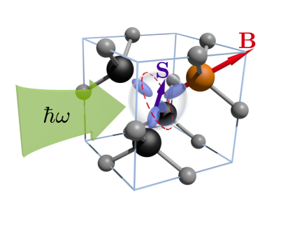
Figure 1: NV-center in diamond with equivalent sp³-hybridized dangling bonds (blue) $\sigma_{i}$ ($i=1,2,3$) from the surrounding carbon atoms (black) and $\sigma_{N}$ from the substitutional nitrogen atom (orange) overlapping within the vacancy (center). The $NV$-axis (long red arrow) defines the $z$-axis of the coordinate system and, due to the zero field splitting determines the quantization axis of the electron spin. The magnetic field $B$ is applied along the NV-axis.

II Model

To model optical spin rotations in an individual NV-center in diamond, we start from the commonly used description that fundamentally involves a total number of six electrons, but can be reduced to an effective two-electron Len ; Man ; Doherty or, equivalently, two-hole model Maze . The four relevant single-electron orbitals $a_{1}$, $a_{2}$, $e_{x}$, and $e_{y}$ can be obtained by projecting the $sp^{3}$-hybridized dangling bonds $\sigma_{1,2,3}$ of the carbon atoms and $\sigma_{N}$ of the nitrogen atom (see Fig. 1) onto the irreducible representations of the $C_{3v}$ symmetry group of the NV center Maze . The electron configurations for the ground and first excited state are obtained as follows: In the ground state ($e^{2}$) configuration, the lower-energy $a_{1,2}$ orbitals are completely filled with two electrons each, while the $e_{x}$ and $e_{y}$ contain one electron each. The two-fold degenerate excited state configuration ($ae$) is obtained by promoting another electron from $a_{1}$ to $e_{x}$ or $e_{y}$. Due to the Coulomb interaction between the two electrons, the spin triplet lies lowest in energy and forms the ground state $e^{2}(T)$, transforming according to the representation $A_{2}$ of $C_{3v}$ Maze . Electric dipole transitions connect this triplet to the excited state spin triplet $ea(T)$, transforming according to the $E$ representation. The two-fold orbital and three-fold spin degeneracies give rise to a total of six states in $ea(T)$, compared to three states in $e^{2}(T)$. The spin singlet states will not be of direct importance for our discussion, and are left out of our model. The entire state space for our model is thus nine-dimensional.

II.1 Ground state

The Hamiltonian of the ground state spin triplet in the basis $\left\{{}^{3}A_{2-},^{3}A_{20},^{3}A_{2+}\right\}=\left\{|-1\rangle,|0\rangle,|+1\rangle\right\}$ is

$$H_{\rm gs}=\begin{pmatrix}D_{\rm gs}-g_{\rm gs}\mu_{B}B&0&0\\ 0&0&0\\ 0&0&D_{\rm gs}+g_{\rm gs}\mu_{B}B\end{pmatrix},$$ (1)

where $B$ denotes an external magnetic field aligned with the $NV$-axis, $g_{\rm gs}$ the Landé g-factor, and $\mu_{B}$ the Bohr magneton. Around the ground-state level anticrossing (LAC), we can split the Zeeman energy into a term that compensates the ground state zero field splitting and an additional variation, $g\mu_{B}B=D_{\rm gs}+g\mu_{B}\delta B$. The zero field splitting $D_{\rm gs}=2.88$ GHz Oort is caused by the reduction of the symmetry in spin space to $C_{3v}$ due to the crystal field. The absence of orbital degeneracy in the ground state triplet implies that strain and spin-orbit interaction have very little effect on the ground state.

Here, we have neglected the effect of the hyperfine coupling to the nuclear spins of the intrinsic nitrogen atom and surrounding ¹³C atoms. If necessary, the nuclear spin state could be prepared optically.

II.2 Excited state

At low temperatures, the excited state fine structure can be understood to a large extent from strain and spin-spin interactions. In the basis of spin-orbit states with full symmetry, described by the $C_{3v}$ double group including spin Maze , $\left\{A_{1},A_{2},E_{X},E_{Y},E_{1},E_{2}\right\}$ the excited-state Hamiltonian matrix is

$$H_{\rm es}=\left(\begin{matrix}D_{\rm es}/3+\Delta+l_{z}&g_{\rm es}\mu_{B}B&0&0&\delta_{x}&-i\delta_{y}\\ g_{\rm es}\mu_{B}B&D_{\rm es}/3-\Delta+l_{z}&0&0&i\delta_{y}&-\delta_{x}\\ 0&0&-2D_{\rm es}/3+\delta_{x}&\delta_{y}&0&\Delta^{\prime\prime}\\ 0&0&\delta_{y}&-2D_{\rm es}/3-\delta_{x}&i\Delta^{\prime\prime}&0\\ \delta_{x}&-i\delta_{y}&0&-i\Delta^{\prime\prime}&D_{\rm es}/3-l_{z}&-g_{\rm es}\mu_{B}B\\ i\delta_{y}&-\delta_{x}&\Delta^{\prime\prime}&0&-g_{\rm es}\mu_{B}B&D_{\rm es}/3-l_{z}\end{matrix}\right),$$ (2)

where $l_{z}$ is the axial spin-orbit splitting, and $D_{\rm es}=-\frac{3}{4}D_{zz}$ and $\Delta=\frac{1}{2}D_{x^{2}-y^{2}}$ are the well-known spin-spin interactions Len . Experimentally, it was found that $l_{z}=5.3$ GHz, $D_{\rm es}=1.42$ GHz and $\Delta=1.55$ GHz Bat . The Landé factors of ground and excited state were found to be equal Fuc ; Neu ; Hem , $g_{\rm gs}\simeq g_{\rm es}\simeq 2.01=g$. The energy gap $E_{g}$ is defined as the difference between the $E_{1,2}$ excited states and the $m_{S}=\pm 1$ ground states at $B=0$. The dependence of the ground- and excited state levels on $B$ is shown in Fig. 2.

Since electric dipole transitions are spin-conserving, our all-optical spin control scheme requires a spin non-conserving mechanism in the excited state. The longitudinal spin-orbit interaction term $l_{z}$ only leads to an additional energy splitting between states with different spin projections and cannot flip the spin. It was speculated that the transversal part of the spin-orbit interaction can lead to spin flips Rog ; Tam , but it has recently turned out that it can only connect orbital states belonging to different irreducible representationsMaze . However, the transversal component $\Delta^{\prime\prime}\simeq 0.2\,{\rm GHz}$ of the spin-spin interaction allows for the non-spin-conserving transitions between the $E$ and $E^{\prime}$ states, explaining the experimentally observed transitionsMaze .

The components $\delta_{x}$ and $\delta_{y}$ of the non-axial strain can be written in polar coordinates, $\delta_{\bot}^{2}=\delta_{x}^{2}+\delta_{y}^{2}$ and $2\beta=\arctan(\delta_{y}/\delta_{x})$. Here, $\beta$ was defined such that it corresponds to the angle between the symmetry axis of strain eigenstates $e_{x}^{\prime}\left(\delta_{x},\delta_{y}\right)$ and the symmetry axis of the unperturbed $e_{x}$-orbital.

II.3 Electric dipole transitions

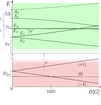
Figure 2: Illustration of the optical pumping process with frequency $\omega$ from $m_{s}=0$ ground state spin level below the excited state. The degenerate $E_{x,y}$ levels are coupled to the $E_{1,2}$ levels by the transversal spin-spin-interaction $\Delta^{\prime\prime}$.

We assume the system to be optically driven with a radiation field at fixed frequency $\omega$ near $E_{g}$, therefore it is convenient to describe the excited states in a corotating frame, while keeping the ground states fixed. We then work in the rotating wave approximation where counter-rotating terms with frequency $E_{g}+\omega$ are neglected. This is justified as long as $\delta\omega=E_{g}-\omega\ll E_{g}$. Optical transitions between the ground and excited state are described with the electric dipole operator for two electrons, $H_{\rm dip}^{(2)}=H_{\rm dip}^{(1)}\otimes\mathbb{1}+\mathbb{1}\otimes H_{\rm dip}^{(1)}$, where

$$H_{\rm dip}^{(1)}=e\mathbf{E}\cdot\hat{\mathbf{r}}=e\left|\mathbf{E}\right|\left(\hat{x}\cos{\alpha}+\hat{y}\sin{\alpha}\right)$$ (3)

is the single-particle electric dipole operator, where $\hat{\mathbf{r}}=(\hat{x},\hat{y},\hat{z})$ denotes the electron position operator. Here, we assumed the incident light to be linearly polarized perpendicular to the $NV$-axis (which defines the $z$-axis of the coordinate system) with polarization angle $\alpha$, with $\alpha=0$ for polarization parallel to the symmetry axis of the $e_{x}$-orbital. Taking matrix elements with the ground and excited state basis states yields the Hamiltonian

$$H=\begin{pmatrix}H_{\rm gs}&0\\ 0&\Delta\omega\mathbb{1}+H_{\rm es}\end{pmatrix}+\begin{pmatrix}0&v\\ v^{\dagger}&0\end{pmatrix}=H_{0}+V,$$ (4)

where the detuning $\delta\omega$ is defined with respect to the lowest-lying excited state energy levels $E_{1,2}$ (neglecting strain and spin mixing $\Delta^{\prime\prime}$), and $\Delta\omega=\delta\omega+l_{z}-\frac{D_{\rm es}}{3}$. The transition matrix is given as

$$v=\begin{pmatrix}i\epsilon_{+}&-i\epsilon_{+}&0&0&-i\epsilon_{-}&-i\epsilon_{-}\\ 0&0&-2\epsilon_{y}&2\epsilon_{x}&0&0\\ -i\epsilon_{-}&-i\epsilon_{-}&0&0&i\epsilon_{+}&-i\epsilon_{+}\end{pmatrix}$$ (5)

where, for linear polarization of the excitation field,

$$\epsilon_{\pm}=\epsilon_{x}\pm i\epsilon_{y}\equiv\epsilon e^{\pm i\alpha},$$ (6)

and ($i=x,y$)

$$\epsilon_{i}=\frac{\left\langle e\right|\left|\hat{r}_{E}\right|\left|a\right\rangle}{4}eE_{i}$$ (7)

with the reduced matrix element of the position operator defined as

$$\left\langle e\right|\left|\hat{r}_{E}\right|\left|a\right\rangle=\left\langle e_{x}\right|\hat{x}\left|a\right\rangle=\left\langle e_{y}\right|\hat{y}\left|a\right\rangle.$$ (8)

We are interested in linearly polarized optical fields, where $\epsilon$ is real. The magnitude of the dipole matrix elements can be estimated from the observed Rabi oscillation period Rob and the linear Stark shift Tam2 , typically $\epsilon\approx 1\,{\rm GHz}$.

III Effective Spin Hamiltonian

III.1 Schrieffer-Wolff transformation

Since the energy levels of the ground state $H_{\rm gs}$ and the excited state $H_{\rm es}$ are widely seperated by $E_{g}=1.945$ eV $\approx 470$ THz and coupled by small perturbations $\epsilon\ll|\delta\omega|=|E_{g}-\omega|$, we can use a Schrieffer-Wolff transformation SW of the Hamiltonian (block-matrix) as a valid approach to determine the effective dynamics of the driven system up to second order in the perturbation. The Schrieffer-Wolff transformation is defined as follows,

$$\tilde{H}=e^{S}He^{-S}=H+\left[S,H\right]+\frac{1}{2}\left[S,\left[S,H]\right]\right]+\mathcal{O}\left(S^{3}\right),$$ (9)

with the anti-hermitian transformation matrix

$$S=\begin{pmatrix}0&s\\ -s^{\dagger}&0\end{pmatrix}.$$ (10)

The aim of the transformation is to remove the coupling $V$ in first order, which can be achieved if $\left[S,H_{0}\right]=-V$. In terms of the submatrices for the two seperated systems $H_{\rm gs}$ and $H_{\rm es}$ and their coupling $V$ this condition reduces to

$$sH_{\rm es}-H_{\rm gs}s=-v,$$ (11)

which also implies that in a perturbation series in $v$, the matrix $s$ will be first order, $s\sim O(v)$. This particular choice of transformation secures that the first order terms in Eq. (9) cancel and we are left with an effective ground-state Hamiltonian

$$\tilde{H}=H_{\rm gs}+\frac{1}{2}\left(s^{\dagger}v+v^{\dagger}s\right)+\mathcal{O}\left(v^{3}\right).$$ (12)

Note that in the absence of strain $l_{z}-D_{\rm es}-D_{\rm gs}\approx 1$ GHz is the seperation between the two closest-lying energy levels $E_{x,y}$ and $E_{+}=E_{1}+E_{2}$, and thus for resonant excitation between those two levels, the optical driving field strength has to be much smaller than $500$ MHz.

III.2 Rotation axis

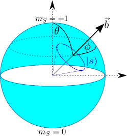
Figure 3: The state $|s\rangle$ of the ground state spin qubit in the $m_{S}=0,-1$ subspace can be represented as a vector on the Bloch sphere where the two poles represent the two Zeeman-split eigenstates $\left|m_{s}=0\right\rangle$ and $\left|m_{s}=-1\right\rangle$. The vector $\mathbf{b}$ denotes the effective magnetic field acting on this pseudo-spin 1/2, with spherical angles $\theta$ and $\phi$.

We focus on the transition between the $m_{S}=-1$ and $m_{S}=0$ ground state spin levels. This two-level system can be split off from the $m_{S}=+1$ state footnote_SW2 , in the regime $g\mu_{B}|\delta B|\lesssim 2D_{\rm gs}$. In this case the dynamics is described by the $2\times 2$ Hamiltonian

$$\tilde{H}=\left(\begin{matrix}\tilde{H}_{11}&\tilde{H}_{12}\\ \tilde{H}_{21}&\tilde{H}_{22}\end{matrix}\right)=b_{0}\openone+\bm{\mathbf{b}}\cdot\bm{\sigma}$$ (13)

where the effective (pseudo-) magnetic field has components,

$$b_{x} = \frac{1}{2}\left(\tilde{H}_{12}+\tilde{H}_{21}\right)=b_{\bot}\cos\phi,$$ (14)

$$b_{y} = \frac{1}{2i}\left(\tilde{H}_{12}-\tilde{H}_{21}\right)=b_{\bot}\sin\phi,$$ (15)

$$b_{z} = \frac{1}{2}\left(\tilde{H}_{11}-\tilde{H}_{22}\right),$$ (16)

and $b_{0}=\tilde{H}_{11}+\tilde{H}_{22}$. The dynamics within this two-dimensional subspace can be visualized using a Bloch sphere picture, as shown in Fig. 3. Optical driving results in a rotation of the state vector about an axis $\mathbf{b}$ with polar angle (axial orientation) $\theta$ and azimuthal angle (non-axial orientation) $\phi$. The transversal part $b_{\bot}=\left|\tilde{H}_{12}\right|=\sqrt{b_{x}^{2}+b_{y}^{2}}=b\sin\theta$ of the effective field provides for effective spin-flip transitions while $b_{z}$ accounts for the effective (AC Stark) splitting between the two levels (around the LAC). The term $\propto\mathbbm{1}$ in Eq. (13) can be omitted since it merely leads to a global phase. The precession frequency is given by

$$b=\sqrt{b_{\bot}^{2}+b_{z}^{2}}=\sqrt{1+\cot^{2}{\theta}}|b_{\bot}|.$$ (17)

Spin flips can be implemented as rotation about an axis within the equatorial plane of the Bloch sphere (Fig. 3) which corresponds to $\theta=\frac{\pi}{2}$ and thus $b=b_{\bot}$.

IV Results

IV.1 Unstrained NV center

In the case of vanishing strain ($\delta_{\bot}=0$) we obtain a simple analytical result for the transversal component of the qubit rotation axis, with magnitude,

$${b}_{\bot} = \Delta^{\prime\prime}\epsilon^{2}\left|\frac{1}{\delta\omega\left(\delta\omega+D_{\rm es}+l_{z}+D_{\rm gs}+g\mu_{B}\delta B\right)}\right.$$

$$\!\!+\left.\frac{1}{\left(\delta\omega-g\mu_{B}\delta B\right)\left(\delta\omega-D_{\rm es}+l_{z}+D_{\rm gs}\right)}\right|+O\!\left(\Delta^{\prime\prime 2}\right)\!,$$

which is proportional to the intensity $\epsilon^{2}$ of the optical driving field and the transversal spin-spin coupling $\Delta^{\prime\prime}$ in the excited state. The azimuthal angle of the rotation axis is determined by the optical polarization angle $\alpha$,

$$\phi=-2\alpha$$ (19)

where the factor of 2 reflects the double group character of spin representation. The polar angle $\theta$ of the rotation axis is independent of $\alpha$ and for small $g\mu_{B}\delta B$ even independent of the driving field strength $\epsilon$. The residual Zeeman splitting is limited by the hyperfine LAC of about $2$ MHzGali , and therefore for an optical coupling $\epsilon\gtrsim 100\,{\rm MHz}$ we can always find pairs of parameters $(\delta B,\delta\omega)$ that fullfill the condition $\theta=\pi/2$.

In the limit of large detuning, i.e., when $\delta\omega$ dominates all other energies in the denominators of Eq. (IV.1), we can approximate the transverse component of the effective field as

$$b_{\bot}\simeq 2\Delta^{\prime\prime}\frac{\epsilon^{2}}{\delta\omega^{2}}.$$ (20)

IV.2 Effect of strain

We now include the effect of strain in the diamond crystal into our discussion. For moderate strain $\delta_{x,y}\ll 2l_{z}\approx 10$ GHz, the $A_{1,2}$ levels of the excited state are largely seperated from the $E_{1,2}$ levels, and thus the strain-induced mixing of $A_{1,2}$ states and $E_{1,2}$ states can be neglected in lowest order.

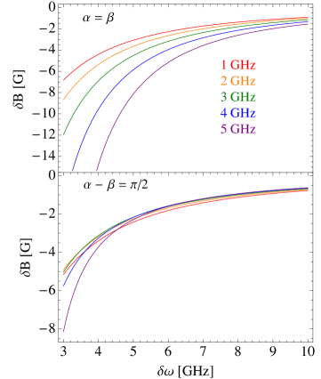
Figure 4: Pairs of required magnetic field variation $\delta B$ and detuning $\delta\omega$ at fixed dipole coupling strength $\epsilon=500\,{\rm MHz}$ for different values of transversal strain $\delta_{\bot}=1,2,3,4$ and $5$ GHz (from top to bottom) to fullfill the condition $\theta=\frac{\pi}{2}$ for precession around a rotation axis within the equatorial plane of the Bloch sphere for $\alpha=\beta=0$.

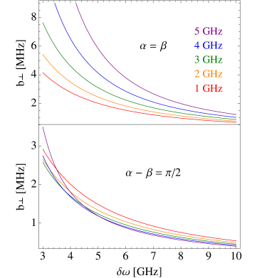
Figure 5: Precession frequency $b_{\bot}$ for different values of transversal strain $\delta_{\bot}=1,2,3,4$ and $5$ GHz (from left to right) for polarization parallel ($\alpha=\beta$) and perpendicular ($\alpha-\beta=\frac{\pi}{2}$) to strain with dipole coupling $\epsilon=500$ MHz.

The main effect of moderate strain is thus a shift of the resonances in Eq. (IV.1) by $\pm\delta_{\bot}=\pm\sqrt{\delta_{x}^{2}+\delta_{y}^{2}}$ , lifting the degeneracy of $E_{x}$ and $E_{y}$ levels. Though strain does not directly mix states with different spin projections, this shift reduces the energetic seperation between coupled $E$ and $E^{\prime}$ levels and therefore strongly enhances the efficiency of spin-flip-transitions.

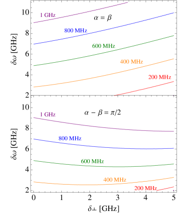
Figure 6: Pairs of detuning $\delta\omega$ and transversal strain $\delta_{\bot}$ that match the condition $\theta=\frac{\pi}{2}$ for precession around a rotation axis within the equatorial plane of the Bloch sphere for different dipole coupling $\epsilon=100,200,400,600,800$ and $1000$ MHz (from bottom to top) for $\alpha=\beta=0$.

In Fig. 4, we plot suitable pairs of parameter values for the detuning $\delta\omega$ (near resonant driving) and Zeeman splitting $g\mu_{B}\delta B$ with varying strain $\delta_{\bot}$ that fulfill the condition $\theta=\frac{\pi}{2}$ for an in-plane rotation axis.

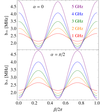
Figure 7: Precession frequency $b_{\bot}$ around in-plane rotation axis at $10$ GHz detuning for optical coupling $\epsilon=500$ MHz and polarization in $e_{x}$ ($\alpha=0$) and $e_{y}$ ($\alpha=\frac{\pi}{2}$) direction for different values of transversal strain $\delta_{\bot}=1,2,3,4,5$ GHz (increasing amplitude) over strain direction angle $\beta$.

This defines an implicit function $\delta B\left(\delta\omega,\delta_{\bot}\right)$ given $\alpha$ and $\beta$, e.g. in the case of $\theta=\pi/2$ for $\alpha=\beta=0$. To find the strength of spin-flip transitions, we substitute $\delta B$ into the precession frequency for an in-plane rotation axis, $b_{\bot}$ and plot it in Fig. 5 as a function of the optical frequency detuning $\delta\omega$ for different values of transversal strain. We find that the precession frequency $b_{\bot}$ indeed increases with strain. Varying $\epsilon$ numerically shows that the precession frequency is still proportional to the intensity of the optical driving field $b_{\bot}|_{\theta=\frac{\pi}{2}}\propto\epsilon^{2}$. Note that the perturbative approach breaks down as detuning approaches strain (divergence of $b_{\bot}$ in Fig.  5), restricted by the validity condition $\delta\omega\ll\delta_{\bot}$ for the Schrieffer-Wolff transformation in Eq. (4). We also investigate the dependence on the direction of strain and polarization (see Fig.  7). Expectedly we get the highest efficiency for collinear strain and polarization and a minimal efficiency for perpendicular relative orientation with an overall sinusoidal form of twofold symmetry. Changing the optical polarization angle $\alpha$ only leads to a uniform and continuous shift of this function (this has been checked for a variety of different values, but for simplicity we only show it for $\alpha=0$ and $\alpha=\frac{\pi}{2}$). Thus, for weak strain, the resulting effective field only depends on the relative angle $\alpha-\beta$ between the strain and polarization angles. However, as the transversal strain $\delta_{\bot}$ increases beyond about $10$ and $20$ GHz, we start observing a modulation of the field with higher harmonics of $\alpha-\beta$.

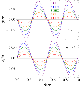
Figure 8: Non axial orientation angle $\phi$ of precession axis for polarization parallel ($\alpha=0$) and perpendicular ($\alpha=\frac{\pi}{2}$) to $e_{x}$-orbitals symmetry axis in respect to strain orientation for different strengths of transversal strain.

Numerical evaluation also reveals that the azimuthal angle (for in-plane orientation of the precession axis) is generally independent of optical coupling strength and magnetic field,

$$\phi=\phi\left(\alpha,\beta,\delta_{\bot},\delta\omega\right).$$ (21)

From Fig. 8 we see that for $e_{x/y}$-polarized light (i.e. $\alpha=0,\frac{\pi}{2}$), the angle $\phi$ is well approximated by $\phi=\mp\hat{\phi}\left(\delta_{\bot},\delta\omega\right)\left(\delta_{\bot},\delta\omega\right)\sin{2\beta}$ (at low strain), with an amplitude proportional to the intensity of the strain,

$$\hat{\phi}=\delta_{\bot}f\left(\delta\omega\right)$$ (22)

In Fig. 9, we show that the sinusoidal shape of $\phi$ as a function of $\alpha$ is slightly distorted for polarization angles $\alpha\neq n\frac{\pi}{2}$, $n\in\mathbb{N}$; we also find that this distortion grows with increasing strain.

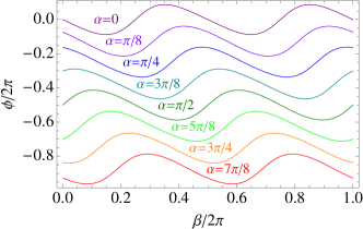
Figure 9: Non axial orientation angle $\phi$ of precession axis for different polarization angles $\alpha$ in respect to strain orientation at transversal strain $\delta_{\bot}=5\,{\rm GHz}$.

IV.3 High strain limit

In the high strain regime, the electronic states of the NV-center are energetically split into two orbital branches with largely seperated energies $E_{x}$ and $E_{y}$ corresponding to a specific choice of coordinate axes, that fixes the orientation angle $\beta$. In this limit $b_{\bot}$ and $b_{z}$ (and thus the polar angle $\theta$) become independent of the orientation angles of both strain and polarization. Expanding in $\delta_{\bot}^{-1}$ yields

$$b_{\bot}\simeq 2\Delta^{\prime\prime}\frac{\epsilon^{2}}{\delta_{\bot}^{2}},$$ (23)

and

$$\phi=2\left(\alpha-2\beta\right)-\frac{\pi}{2}+\mathcal{O}\left(\frac{1}{\delta_{\bot}}\right).$$ (24)

for the transversal part of the pseudo-field, and

$$b_{z}=-\frac{g\mu_{B}\delta B}{2}+2\left(D_{\rm es}-D_{\rm gs}\right)\frac{\epsilon^{2}}{\delta_{\bot}^{2}}+\mathcal{O}\left(\frac{1}{\delta_{\bot}^{3}}\right),$$ (25)

for the longitudinal part. The higher orders contain higher harmonics, such as terms $\propto\Delta\cos{2\left(\alpha-3\beta\right)}$ for $b_{x}$ and $\propto\Delta\sin{2\left(\alpha-3\beta\right)}$ for $b_{y}$ in $\mathcal{O}\left(\frac{1}{\delta_{\bot}^{3}}\right)$, indicating strain induced third order transitions mediated by the $A_{1,2}$ levels.

V Conclusion

We have shown that the effective precession axis and frequency of the ground state spin of the $NV^{-}$-center can be fully controlled by off-resonant optical excitation, by adjusting the frequency detuning $\delta\omega$ and linear polarization angle $\alpha$ of the optical driving field for a given intensity $\epsilon$ (optical dipole coupling) and magnetic field $B$. The orientation of the precession axis is determined by two angles $\theta$ and $\phi$, where the first is depending on all parameters (including strain and polarization) and the latter is independent of magnetic field and optical coupling strength and basically controlled by polarization and strain. The strain effects can be compensated by external bias voltage Bassett2011 . Since any unitary qubit operation (rotation around axis $\mathbf{n}$ by angle $\gamma$) can be composed by successive rotations around two orthogonal axes on the Bloch sphere, a complete set of single-qubit operations can be generated optically in this way. From a purely geometric point of view, spin rotation about an axis within the equatorial plane of the Bloch sphere (where $b_{z}=0$) is most effective for flipping the spin, although any axis other than the $z$-axis would do (the smaller the polar angle $\theta$, the more pulses are be required). A full spin-flip is obtained by a $b_{\bot}\tau=\pi$-rotation around an axis within the equatorial $(x,y)$-plane of the Bloch sphere, providing an estimate for the gate switching (optical pumping) time $\tau$ in the limit of large detuning and weak strain,

$$\tau\simeq\frac{\pi}{2}\frac{\delta\omega^{2}}{\Delta^{\prime\prime}\epsilon^{2}}.$$ (26)

The switching time for spin-flip transitions is limited by the spin mixing term $\Delta^{\prime\prime}$, since the (above) condition implies via the off-resonant condition $\epsilon\ll\delta\omega$ the following lower limit for the spin-flip,

$$\tau\gtrsim\frac{\pi}{\Delta^{\prime\prime}}\approx 10\,\mathrm{ns}$$ (27)

where for that latter estimate we assumed $\Delta^{\prime\prime}=0.2$ GHz.

References

- (1) R. Hanson and D. D. Awschalom, Nature 453, 1043 (2008).
- (2) F. Jelezko, T. Gaebel, I. Popa, A. Gruber, J. Wrachtrup, Phys. Rev. Lett. 92, 076401 (2004).
- (3) T. A. Kennedy, J. S. Colton, J. E. Butler, R. C. Linares, and P. J. Doering, Appl. Phys. Lett. 83, 4190 (2003).
- (4) R. Hanson, O. Gywat, and D. D. Awschalom, Phys. Rev. B 74, 161203(R) (2006).
- (5) D. M. Toyli, D. J. Christle, A. Alkauskas, B. B. Buckley, C. G. Van de Walle, D. D. Awschalom, arXiv:1201.4420 (2012).
- (6) G. Balasubramanian et al., Nature Materials 8, 383 (2009).
- (7) G. Davies and M.F. Hamer, Proc. R. Soc. A, 348, 28 (1976).
- (8) A. Gruber, A. Drabenstedt, C. Tietz, L. Fleury, J. Wrachtrup, and C. Borczyskowski, Science 276, 2012 (1997).
- (9) J. H. H. Loubser and J. A. van Wyk, Diamond Res. 1, 11 (1977).
- (10) J. Harrison, M. J. Sellars, N. B. Manson, J. Lumin. 107, 245 (2004).
- (11) J. Harrison, M. J. Sellars, N. B. Manson, Diamond Rel. Mater. 15, 586 (2006).
- (12) N. Manson, J. Harrison, M. Sellars, Phys. Rev. B 74, 104303 (2006).
- (13) M. H. Mikkelsen, J. Berezovsky, N. G. Stoltz, L. A. Coldren, and D. D. Awschalom, Nature Physics 3, 770 (2007).
- (14) J. Berezovsky, M. H. Mikkelsen, N. G. Stoltz, L. A. Coldren, D. D. Awschalom, Science 320, 349 (2008).
- (15) B. B. Buckley, G. D. Fuchs, L. C. Bassett, and D. D. Awschalom, Science 330, 1212 (2010).
- (16) E. Togan, Y. Chu, A. Imamoglu, and M. D. Lukin, Nature 478, 497 (2011).
- (17) C. Santori, P. Tamarat, P. Neumann et al., Phys. Rev. Lett. 97, 247401 (2006).
- (18) X. F. He, N. Manson, P. Fisk, Phys. Rev. B 47, 8809 (1993).
- (19) A. Lenef, S. Rand, Phys. Rev. B 53, 13441 (1996).
- (20) M. W. Doherty, N. B. Manson, P. Delaney, and L. C. L. Hollenberg, New J. Phys. 13, 025019 (2011).
- (21) J. R. Maze, A. Gali, E. Togan, Y. Chu, A. Trifonov, New J. Phys. 13, 025025 (2011).
- (22) E. van Oort, N. B. Manson, and M. Glasbeek, J. Phys. C 21, 4385 (1988).
- (23) L. Rogers, M. McMurtie, M. Sellars et al., New J. Phys. 11, 063007 (2009).
- (24) P. Tamarat, N. Manson, J. Harrison et al., New J. Phys. 10, 045004 (2008).
- (25) A. Batalov, V. Jacques, F. Kaiser, P. Siyushev, P. Neumann, Phys. Rev. Lett. 102, 195506 (2009).
- (26) G. D. Fuchs, V.V. Dobrovitski, R. Hanson, A. Batra, C. D. Weis, T. Schenkel, D. D. Awschalom, Phys. Rev. Lett. 101, 117601 (2008).
- (27) P. Neumann, R. Kolesov, V. Jacques, J. Beck, J. Tisler, New J. Phys. 11, 013017 (2009).
- (28) P. Hemmer, R. Turukhin, A. V. Shahriar, M. S. Musser, J. A., Opt. Lett. 26, 361 (2001).
- (29) J. Schrieffer and P. Wolff, Phys. Rev. 149, 491 (1966).
- (30) This can be justified by a second Schrieffer-Wolff transformation.
- (31) R. Hanson, F. Mendoza, R. Epstein, D. Awschalom, Phys. Rev. Lett. 97, 087601 (2006).
- (32) F. Jelezko, I. Popa, A. Gruber, C. Tietz, J. Wrachtrup, Appl. Phys. Lett. 81, 2160 (2002).
- (33) A. Gali, M. Fyta, E. Kaxiras, Phys. Rev. B 77, 155206 (2008).
- (34) N. B. Manson, J. P. Harrison, and M. J. Sellars, arXiv:cond-mat/ 0601360 (2006).
- (35) A. Lenef and S. Brown, D. Redman, S. Rand, J. Shigley, E. Fritsch, Phys. Rev. B 53, 13427 (1996).
- (36) L. Robledo, H. Bernien, I. van Weperen, R. Hanson, Phys. Rev. Lett. 105, 177403 (2010).
- (37) P. Tamarat, T. Gaebel, J. Rabeau, M. Khan, A. Greentree, Phys. Rev. Lett. 97, 083002 (2006).
- (38) L. C. Bassett, F. J. Heremans, C. G. Yale, B. B. Buckley, and D. D. Awschalom, Phys. Rev. Lett. 107, 266403 (2011).