Undamped electrostatic plasma waves

Abstract

Electrostatic waves in a collision-free unmagnetized plasma of electrons with fixed ions are investigated for electron equilibrium velocity distribution functions that deviate slightly from Maxwellian. Of interest are undamped waves that are the small amplitude limit of nonlinear excitations, such as electron acoustic waves (EAWs). A deviation consisting of a small plateau, a region with zero velocity derivative over a width that is a very small fraction of the electron thermal speed, is shown to give rise to new undamped modes, which here are named corner modes. The presence of the plateau turns off Landau damping and allows oscillations with phase speeds within the plateau. These undamped waves are obtained in a wide region of the $(k,\omega_{{}_{R}})$ plane ($\omega_{{}_{R}}$ being the real part of the wave frequency and $k$ the wavenumber), away from the well-known ‘thumb curve’ for Langmuir waves and EAWs based on the Maxwellian. Results of nonlinear Vlasov-Poisson simulations that corroborate the existence of these modes are described. It is also shown that deviations caused by fattening the tail of the distribution shift roots off of the thumb curve toward lower $k$-values and chopping the tail shifts them toward higher $k$-values. In addition, a rule of thumb is obtained for assessing how the existence of a plateau shifts roots off of the thumb curve. Suggestions are made for interpreting experimental observations of electrostatic waves, such as recent ones in nonneutral plasmas.

I Introduction

In his 1946 seminal paper landau46 Landau demonstrated that electrostatic plasma waves of vanishing amplitude can be damped, due to their interaction with particles that stream with velocities close to the wave phase speed, $v_{\phi}$. For unmagnetized uniform plasmas, the wave damping rate is generally proportional to the slope of the equilibrium distribution of particle velocities at $v_{\phi}$. Therefore, for monotonically decreasing equilibrium velocity distribution functions (such as the usual Maxwellian) plasma waves are damped exponentially in time.

Almost twenty years later O’Neil oneil65 analyzed the effects of nonlinearity on the propagation of plasma waves and found that the process of particle trapping in the wave potential well can inhibit Landau damping, by flattening the velocity distribution near the wave phase speed.

In 1991 Holloway and Dorning holloway91 noted that certain nonlinear electrostatic oscillations can survive Landau damping even when their phase velocities are comparable to the electron thermal speed, $v_{th}$, due to the effect of particle trapping. They called these waves electron acoustic waves (EAWs), since in the range of small wavenumbers their dispersion relation is of the form $\omega\simeq 1.31kv_{th}$. An EAW is in fact a Bernstein-Greene-Kruskal (BGK) mode bernstein57 with a velocity distribution function that is effectively flat at the wave phase speed, due to trapping. In 1991, Demeio and Holloway demeio91 performed Vlasov-Poisson simulations and provided evidence for the analytical results of Ref. holloway91 . Also in Ref. holloway91 , the authors claimed that these undamped plasma oscillations have no linear counterpart, since in their construction the trapped particle distribution vanishes with wave amplitude and approaches a Maxwellian, for which the waves are heavily damped.

The latter point was discussed in 1994 by Shadwick and Morrison shadwick94 , where it was pointed out that stationary inflection point modes are the natural linear limit of the EAWs (BGK modes) of Ref. holloway91 . A stationary inflection point mode is an undamped mode with phase speed $v_{\phi}$ at a point where the first two derivatives of a stable homogeneous equilibrium velocity distribution function vanish, and by the Penrose criterion this is necessary for the simultaneous existence of the mode and stability. The issue here is that the homogeneous equilibrium distribution function approached as the wave amplitude approaches zero is not unique, and there is no a priori reason it should be locally Maxwellian, since the structure near $v_{\phi}$ is determined by the history of formation of the waves. Given a nonlinear BGK wave, there are many ways the limit of the vanishing of trapped particles can be taken and the result is clearly norm dependent. (See Ref. hagstrom for a discussion of bifurcations in $W^{1,1}$.)

The existence of the EAW branch has been investigated in many electrostatic Particle-In-Cell valentini06 and Vlasov-Poisson afeyan04 ; johnston09 simulations. Moreover, recent Vlasov-Yukawa simulations (with Vlasov ions and linear adiabatic electrons) led to the prediction of undamped electrostatic waves at low frequencies (of the order of the proton plasma frequency), similar in nature to the EAWs and dubbed ion-bulk waves valentini111 ; valentini112 . EAW-type fluctuations have been detected in spacecraft data from observations in the interplanetary medium gary85 . Also, the excitation of the EAWs has been obtained in laboratory experiments with nonneutral plasmas anderegg091 ; anderegg092 , in which an external driving electric field is applied to the plasma column for the time needed to create a population of trapped particles, with the waves surviving after the drive is turned off. The flat region in the particle velocity distribution generated by trapping at the wave phase speed inhibits Landau damping and allows the EAWs to survive. The experimental results discussed in Refs. anderegg091 ; anderegg092 confirm the existence of EAWs on the nonneutral analog of the so-called thumb curve of Ref. holloway91 , as is the case for the numerical results in Refs. afeyan04 ; valentini06 ; johnston09 ; however, these experiments also suggest that wave excitation can be obtained off of the usual thumb curve of Ref. holloway91 , which we will refer to as off-dispersion EAWs. The purpose of this paper is to shed some light on the nature of these off-dispersion EAWs, by examining the sensitivity of the thumb curve to small deviations from the Maxwellian used in Ref. holloway91 .

However, before starting our analysis, we note that in a separate research thread, motivated by experiments on nonlinear laser plasma interactions mont02 , Afeyan and collaborators afeyan04 ; johnston09 carried out extensive Vlasov simulations and observed states that they referred to as Kinetic Electrostatic Electron Nonlinear (KEEN) waves. These large amplitude structures also exist off-dispersion; however, the KEEN waves observed by these authors are large amplitude, while we focus on relatively low amplitude EAWs, where any effect of nonlinearity is limited to a narrow velocity range of trapped particles.

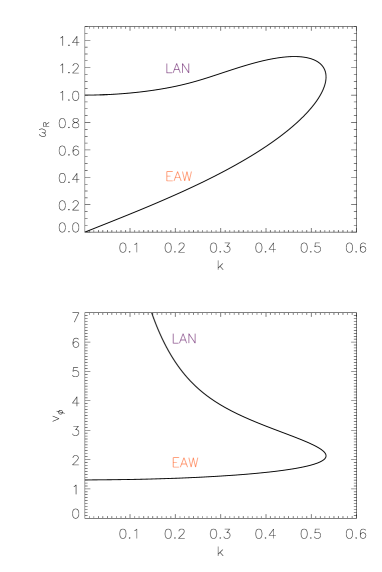
Figure 1: Thumb curve in the $k-\omega_{{}_{R}}$ plane displaying branches of undamped LAN waves and EAWs (top). The same thumb curve plotted in the $k-v_{\phi}$ plane (bottom).

Specifically, we investigate both on-dispersion and off-dispersion EAWs with a simple linear dispersion analysis. As noted above, there is no a priori reason the distribution in the vicinity of $v_{\phi}$ should be Maxwellian, since the structure near $v_{\phi}$ is determined by the history of formation of the waves, and since experimentally fine details of the distribution function are difficult to measure, it is natural to examine the alteration of the thumb curve of Ref. holloway91 caused by small deviations from the Maxwellian. Of main importance here is the alteration caused by replacing the trapped particle region of the velocity distribution by a plateau, but we also consider the alteration caused by altering the tail of the distribution function.

For the plateau distribution function (see Eq. (3)) the Landau velocity integral is carefully evaluated using a high resolution trapezoidal scheme. We look for roots of the dispersion function in the high frequency range of electron modes, treating the ions as a stationary neutralizing background charge. Consistent with the experiments anderegg091 ; anderegg092 the analysis shows that undamped EAWs exist in a wide range of the $(k,\omega_{{}_{R}})$ plane, that is, off the thumb curve of holloway91 .

From the perspective of the linear dispersion analysis, the existence of the off-dispersion modes is easy to understand. The Landau velocity integral in the dielectric function obtains contributions from velocities that are well away from the plateau (the non-resonant particle contributions) and contributions from near the plateau (the resonant particle contributions). The thumb dispersion curve is determined exclusively by contributions from the non-resonant particles, that is, for $(k,\omega_{{}_{R}})$ on the dispersion curve, the non-resonant contribution alone yields a dielectric function that is zero. Off the dispersion curve, the non-resonant contribution yields a dielectric function that is not zero, so the resonant contribution must make up the difference, yielding a total dielectric function that is zero. Thus, for the off-dispersion modes, electrons in the resonant (or plateau) region make a significant contribution to the mode charge density. In that sense, the off-dispersion modes are like beam modes, for which a significant part of the charge density resides on the beam oneil68 . As we will see, for the case of the plateau (rather than a beam), the resonant particle charge density is associated with the two corners of the plateau. Thus, we call these waves corner modes.

As one would expect, the charge density from the corners is a very sensitive function of $v_{\phi}$ in the plateau region. Equivalently, the dielectric function has a spiky variation for $v_{\phi}$ in the plateau region. Thus, a small change in $v_{\phi}$ can make the resonant particle charge density have whatever value is needed to compensate for the non-zero value of the non-resonant dielectric, yielding a total dielectric that is zero. On-dispersion EAWs are special only in that the charge density from the two corners is equal and opposite adding to zero. This is the case if the phase velocity is equidistant from the two corners, that is, at the velocity mid-point of the plateau. From this perspective, there is little difference between the on-dispersion and off-dispersion EAWs. However, there is a significant difference between the EAWs (or corner modes) and weakly damped Langmuir waves, where $v_{\phi}$ is well out on the tail of the velocity distribution and there is no significant corner contribution to the mode charge density.

Another way to obtain off-dispersion waves is to alter the tail of the distribution function, which may not be known precisely. Although the dispersion curve is not as sensitive to this kind of deviation, one can ascertain systematic shift of roots off of the thumb curve. In particular, we can show analytically that a fattening of the tail of the distribution shifts roots toward lower $k$-values and chopping the tail shifts them toward higher $k$-values. Chopping produces perturbed corner charge and this idea leads to a derivation of a rule of thumb for assessing shifts caused by general plateau type of equilibrium distribution functions.

The paper is organized as follows. In Section II we numerically analyze the roots of the electrostatic dielectric function and discuss the wave dispersion relation for a velocity distribution flattened in a small velocity interval. This is followed by an analysis of the consequences of altering the tail and the derivation of the rule of thumb. In Section III the numerical results of Vlasov-Poisson simulations are presented and compared to the analytical predictions of Section II for the plateau distributions. Summary and Conclusions are given in Section IV.

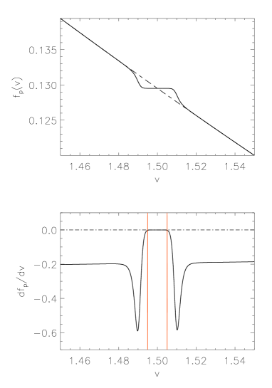
Figure 2: Velocity dependence of the function $f_{p}$ (top) and its first velocity derivative $df_{p}/dv$ (bottom) in the region near $V_{0}=1.50$. Dashed line of top plot is the usual Maxwellian, $f_{{}_{M}}$; red-vertical lines of the bottom plot mark the edges of the interval $[V_{0}-\Delta V_{p}/2,V_{0}+\Delta V_{p}/2]$.

II Wave dispersion relation

The propagation of electrostatic waves in a collisionless unmagnetized plasmas can be described by a simplified 1+1+1 (one space, one velocity, and one time dimension) Vlasov-Poisson system, which is given in dimensionless form as follows:

$$\frac{\partial f}{\partial t}+v\frac{\partial f}{\partial x}-E\frac{\partial f}{\partial v}=0\,,\qquad\frac{\partial E}{\partial x}=1-\int fdv\,,$$ (1)

where $f=f(x,v,t)$ is the electron distribution function and $E=E(x,t)$ the electric field. In (1), the ions are a neutralizing background of constant density $n_{0}=1$, time is scaled by the inverse electron plasma frequency $\omega_{p}^{-1}$, velocities by the electron thermal speed $v_{th}$, and lengths by the electron Debye length $\lambda_{D}$. For simplicity, all the physical quantities will be expressed in these characteristic units.

By linearizing Eqs. (1) and following the Landau prescription landau46 ; krall86 for weak wave damping, the time asymptotic solution for the complex frequency of the fluctuations ($\omega=\omega_{{}_{R}}+i\omega_{{}_{I}}$) can be obtained by looking for the roots of the dielectric function $D(k,\omega)\simeq D_{{}_{R}}(k,\omega_{{}_{R}})+iD_{{}_{I}}(k,\omega_{{}_{R}})+i\omega_{{}_{I}}\partial D_{{}_{R}}(k,\omega_{{}_{R}})/\partial\omega_{{}_{R}}$, where

$$D_{{}_{R}}=1-\frac{1}{k^{2}}\mathchoice{{\vbox{\hbox{$\textstyle-$ }}\kern-6.52776pt}}{{\vbox{\hbox{$\scriptstyle-$ }}\kern-4.91667pt}}{{\vbox{\hbox{$\scriptscriptstyle-$ }}\kern-3.95833pt}}{{\vbox{\hbox{$\scriptscriptstyle-$ }}\kern-3.54166pt}}\!\!\int\!dv\,\frac{f_{0}^{\prime}}{v-v_{\phi}}\,,\qquad D_{{}_{I}}=-\frac{\pi}{k^{2}}\left.f_{0}^{\prime}\right|_{v_{\phi}}\,.$$ (2)

Here, $f_{0}^{\prime}(v):=\partial f_{0}/\partial v$, $\mathchoice{{\vbox{\hbox{$\textstyle-$ }}\kern-6.52776pt}}{{\vbox{\hbox{$\scriptstyle-$ }}\kern-4.91667pt}}{{\vbox{\hbox{$\scriptscriptstyle-$ }}\kern-3.95833pt}}{{\vbox{\hbox{$\scriptscriptstyle-$ }}\kern-3.54166pt}}\!\!\int$ indicates an integral over all $v\in\mathbb{R}$ with the singularity handled by taking the Cauchy principal value, $f_{0}$ is the equilibrium velocity distribution of electrons, and $v_{\phi}=\omega_{{}_{R}}/k$ is the wave phase speed. The roots of $D_{{}_{R}}$ give the real part of the wave frequency $\omega_{{}_{R}}$, while the imaginary part is given by $\omega_{{}_{I}}=-D_{{}_{I}}/(\partial D_{{}_{R}}/\partial\omega_{{}_{R}})$.

Undamped waves can be obtained from Eqs. (2) by assuming $f_{0}$ has a velocity plateau of vanishing velocity width at $v=v_{\phi}$. This renders $D_{{}_{I}}(v_{\phi})=0$ and solution of $D_{{}_{R}}=0$ yields $\omega_{{}_{R}}=\omega_{{}_{R}}(k)$. In Ref. holloway91 , the equation $D_{{}_{R}}=0$ was solved by assuming Maxwellian $f_{0}$ with the velocity plateau of vanishing width, leading to the so-called thumb curve, the dispersion diagram displayed in the top plot of Fig. 1. The upper branch of this $k-\omega_{{}_{R}}$ diagram represents Langmuir (LAN) waves, while modes of the lower branch are usually referred to as EAWs, since for small wavenumbers on the lower branch $\omega_{{}_{R}}^{{}^{(EAW)}}\approx 1.31k$, which is reminiscent of acoustic waves. In the bottom plot of Fig. 1, the same thumb curve is displayed in the $k-v_{\phi}$ plane.

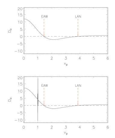
Figure 3: Real part of the dielectric function $D_{{}_{R}}$ as a function of $v_{\phi}$ for $k=0.3$ for a Maxwellian equilibrium velocity distribution (top) and for the equilibrium distribution $f_{p}$ given in Eq. (3) for $V_{0}=1$ (bottom).

From the plots in Fig. 1 it is evident that no undamped roots of $D_{{}_{R}}$ exist beyond a critical value of the wavenumber $k^{*}\simeq 0.53$. The presence of this nose-like structure at $k\simeq k^{*}$ appears unphysical, since the group velocity of the wave at $k^{*}$ seems to diverge. To understand this apparent paradox one should bear in mind that the thumb curve does not represent a usual dispersion relation: each point in the $(k,\omega_{{}_{R}})$ plane along the thumb curve corresponds to a different particle velocity distribution function. In order to get undamped solutions, the location of the infinitesimal plateau in the electron velocity distribution must slide along and always fall at $v=v_{\phi}$. This corresponds to changing the shape of the velocity distribution at each $v_{\phi}$.

As discussed in Sec. I, the existence of the EAW branch has been reproduced in numerical simulations and observed in experiments on nonneutral plasmas. In the experiments, stable oscillations also are observed off-dispersion, i.e., off of the usual thumb curve. In order to obtain insight for understanding this experimental behavior, we will analyze the roots of $D_{{}_{R}}$ for an equilibrium particle velocity distribution function that deviates from Maxwellian by a small, but not infinitesimal, velocity plateau of width $\Delta V_{p}$ located at $v=V_{0}$. Specifically, we chose the plateau distribution function given by

$$f_{p}(v)=N\left(f_{{}_{M}}(v)-\frac{f_{{}_{M}}(v)-f_{{}_{M}}(V_{0})}{1+[(v-V_{0})/\Delta V_{p}]^{n_{p}}}\right)\,,$$ (3)

where $f_{{}_{M}}=\exp{(-v^{2}/2)}/\sqrt{2\pi}$ is the usual Maxwellian, $n_{p}$ is an even integer (here $n_{p}=10$), $\Delta V_{p}=0.01$, and $N$ is a normalization constant that deviates slightly from unity. It is worth noting that $f_{p}$ is smooth in $v$ with derivatives up to order $n_{p}$ that vanish at $v=V_{0}$.

The distribution $f_{p}$ and its first derivative $df_{p}/dv$ are shown in Fig. 2, in the region near $V_{0}$ (where $V_{0}=1.5$ for illustrative purposes); the dashed line in the top plot represents the function $f_{{}_{M}}$. The red-vertical lines in the bottom plot indicate the width of the plateau $\Delta V_{p}$. It is clear from this figure that in the interval $[V_{0}-\Delta V_{p}/2,V_{0}+\Delta V_{p}/2]$ the first velocity derivative of $f_{p}$ obtains very small values.

We investigate the possibility of getting undamped (or weakly damped) plasma oscillations with $v_{\phi}$ in the interval $[V_{0}-\Delta V_{p}/2,V_{0}+\Delta V_{p}/2]$. In this velocity interval, one can numerically calculate the value of $D_{{}_{R}}$ for a fixed $k$, with the imaginary part of the dielectric function being negligible because of the plateau of width $\Delta V_{p}$ at $v=V_{0}$ (see the bottom plot of Fig. 2).

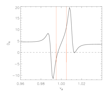
Figure 4: A zoom of the bottom plot of Fig. 3 near $v_{\phi}=V_{0}=1$.

To calculate the value of $D_{{}_{R}}$, we compute the Cauchy principal value of the integral of $D_{{}_{R}}$ of Eqs. (2) on a uniform velocity grid with a standard trapezoidal scheme. The limits of numerical integration are set to $|v_{{}_{max}}|=6$, with the distribution set to zero outside this interval. To smoothly resolve the small plateau of width $\Delta V_{p}=0.01$ in $f_{p}$, in this interval we use a large number of grid points $N_{v}=12000$, so as to have $\Delta v=2|v_{{}_{max}}|/N_{v}=0.001<\Delta V_{p}$.

The two plots of Fig. 3 depict the dependence of $D_{{}_{R}}$ on $v_{\phi}$, for a fixed value of the wavenumber $k=0.3$. In the top plot we show the case where $f_{0}$ is Maxwellian, results which are essentially equivalent to the thumb curve of Fig. 1. In the bottom plot of Fig. 3 we show the results obtained when the equilibrium distribution is chosen to be $f_{p}$ of Eq. (3) with a small plateau at $v=V_{0}=1$. The curve in the top plot displays two roots, the EAW with $v_{\phi}^{{}^{(EAW)}}\simeq 1.44$ and the LAN wave with $v_{\phi}^{{}^{(LAN)}}\simeq 3.86$, both being undamped since $D_{{}_{I}}$ is assumed to vanish at each $v_{\phi}$. Note, the curve in the bottom plot reveals new features: the two roots corresponding to the EAW and LAN wave (in agreement with those of the top plot) now undergo Landau damping (very strong for the EAW), since the location of the velocity plateau in $f_{p}$ is now fixed at $v=V_{0}=1$. In addition, $D_{{}_{R}}$ displays a marked spike in the region around $v_{\phi}\simeq V_{0}=1$.

In Fig. 4 we zoom in for a close-up of the spike region around $V_{0}$ and find several extra roots of $D_{{}_{R}}$. Among these roots, we focus on the one that falls within the interval $[V_{0}-\Delta V_{p}/2,V_{0}+\Delta V_{p}/2]$ marked by the red-vertical lines, since the other roots outside this interval are very strongly Landau damped. Now the search for the undamped root of $D_{{}_{R}}$ and related analysis can be restricted to a limited and very small region of the velocity domain, and we can increase the velocity resolution by a factor of $100$ so as to determine more precisely the location of the root of $D_{{}_{R}}$ in the interval $[V_{0}-\Delta V_{p}/2,V_{0}+\Delta V_{p}/2]$. By doing this, we find that the root of $D_{{}_{R}}$ is located at $v_{\phi}=v_{\phi}^{*}\simeq 0.9966$. We also evaluated the corresponding imaginary part of the dielectric function from the second of Eqs. (2), getting a small value $D_{{}_{I}}\simeq 2\times 10^{-3}$. Moreover, using $\omega_{{}_{R}}=kv_{\phi}^{*}$ and $\omega_{{}_{I}}=-kD_{{}_{I}}/(\partial D_{{}_{R}}/\partial v_{\phi})|_{v_{\phi}^{*}}$, the ratio $R_{th}:=|\omega_{{}_{I}}/\omega_{{}_{R}}|\simeq 10^{-6}$, meaning that this is an almost undamped solution. It is interesting to point out that if one chooses the value of $V_{0}$ (the location of the plateau in $f_{p}$) so that for a fixed $k$ it falls exactly on the thumb curve of Fig. 1 (i.e., it falls exactly on the LAN or EAW branch), the roots of $D_{{}_{R}}$ are found exactly at $v_{\phi}=V_{0}$ and they are completely undamped, since $(df_{p}/dv)_{v=v_{\phi}=V_{0}}=0\Rightarrow D_{{}_{I}}=0$.

In order to establish the domain of parameters for which electrostatic waves can exist without being Landau damped, by including small plateaus in the equilibrium velocity distribution, we calculate the minimum value of $|D_{{}_{R}}|$ in the velocity interval $[V_{0}-\Delta V_{p}/2,V_{0}+\Delta V_{p}/2]$ for different values of $k$ and $V_{0}$. Then $\min{\{|D_{{}_{R}}|\}}=0$ corresponds to a root of $D_{{}_{R}}$.

The results for $\min{\{|D_{{}_{R}}|\}}$ are displayed in the $k-V_{0}$ contour plot of Fig. 5. Here, the dark area represents the region where $\min{\{|D_{{}_{R}}|\}}=0$, which corresponds to weakly damped solutions, while outside this region $\min{\{|D_{{}_{R}}|\}}>0$, which means no solutions exist. The red-dashed line represents the thumb curve previously shown in the bottom plot of Fig. 1. For the dark region of the contour plot in Fig. 5, for which the roots of $D_{{}_{R}}$ are in the interval $[V_{0}-\Delta V_{p}/2,V_{0}+\Delta V_{p}/2]$, one can evaluate the ratio $R_{th}$ to ascertain the importance of Landau damping for each solution. The maximum value of this ratio in the dark region of the contour plot in Fig. 5 is $R_{th}^{{}^{max}}:=\max{\{|\omega_{{}_{I}}/\omega_{{}_{R}}|\}}\simeq 6\times 10^{-5}$, with $|\omega_{{}_{I}}/\omega_{{}_{R}}|$ being exactly null on the thumb curve (red-dashed line in Fig. 5). Therefore, Fig. 5 shows that almost undamped oscillations can be obtained with a small plateau in the equilibrium velocity distribution in an unexpectedly wide region around the thumb curve. More importantly, undamped solutions can be found well beyond the critical wavenumber $k^{*}$ predicted by the thumb curve, suggesting an avenue for understanding the experimental results with nonneutral plasmas discussed in Refs. anderegg091 ; anderegg092 .

To complete our analysis, we analyze the perturbed distribution function of these undamped oscillations, the form of which is given by $\delta f_{p}=f^{\prime}_{p}/(v-v_{\phi}^{*})$ krall86 ; shadwick94 . We first assume $k=0.3$ and $V_{0}=1$ (as in Fig. 3) and $v_{\phi}^{*}=0.9966$, which corresponds to a mode that is located off the thumb curve (see Fig. 1). In the top plot of Fig. 6, $\delta f_{p}$ is plotted as a function of $v$ in the region around $V_{0}=1$. The red-vertical lines mark the interval $[V_{0}-\Delta V_{p}/2,V_{0}+\Delta V_{p}/2]$ and a small spike is seen at the location of the pole at $v=v_{\phi}^{*}=0.9966$. In addition, two pronounced peaks, visible within a velocity interval $I_{v}$ of width $\sim 0.04$ around $V_{0}$, correspond to the sharp corners at the boundaries of the plateau. For this off-dispersion mode, the contributions to $\delta f_{p}$ due to the two corners are not symmetric, because the wave phase speed is not in the center of the velocity plateau, $V_{0}$. This means that for these off-dispersion modes, when $\delta f_{p}$ is integrated over $I_{v}$ there will be a net contribution from the corners to the charge density.

The situation is different for modes that fall on the thumb curve. The bottom plot of Fig. 6 displays $\delta f_{p}$ for an on-dispersion mode with $k=0.4$ and $V_{0}=1.561$. As discussed previously, when the values of $k$ and $V_{0}$ are such that the mode falls on the thumb curve, then $v_{\phi}$ exactly equals $V_{0}$, the center of the velocity plateau. This suppresses the pole in the perturbed distribution (which is valid for any distribution with a plateau at $v=V_{0}$, whose first and second velocity derivatives vanish at $v=V_{0}$). Indeed, the Landau pole is not visible in the bottom plot of Fig. 6 and now the contributions from the two corners are exactly symmetric (but of opposite sign). Consequently, the peaks corresponding to the two corners cancel upon integration over $I_{v}$, yielding a negligible contribution to the charge density.

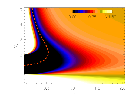
Figure 5: Contour plot of $\min{\{|D_{{}_{R}}|\}}$ in the $k-V_{0}$ plane; red-dashed line is the thumb curve.

In reality, the tail of $f_{p}$ of Eq. (3) is composed of a part that is algebraic and a part that is Maxwellian. This deviation from Maxwellian only matters for large velocities, and it is insignificant for our simulations of Sec. III, where the tail is actually chopped at large velocities. However, it does raise the question of how altering the tail affects the thumb curve. To address this kind of deviation consider an equilibrium of the form $f_{0}(v)=N_{1}f_{{}_{M}}+N_{2}f_{\rm tail}$, where $N_{1}$ and $N_{2}$ are yet to be determined normalization constants, and assume

$$f_{\rm tail}=\left\{\begin{array}[]{cc}f_{{}_{M}}&\quad{\rm for}\ \ v\leq v_{*}\\ \phi_{\rm tail}&\quad\ {\rm for}\ \ v>v_{*}\,,\end{array}\right.$$ (4)

where $v_{*}>v_{\phi}>0$, and we assume continuity at $v_{*}$, but smoothness is not essential. Normalization requires

$$1=N_{1}+N_{2}+N_{2}\,\Delta(v_{*}):=N_{1}+N_{2}+N_{2}\int^{\infty}_{v_{*}}\!dv\,\left(\phi_{\rm tail}-f_{{}_{M}}\right)\,.$$ (5)

Then, the thumb curve is given by

$$k^{2}=\mathchoice{{\vbox{\hbox{$\textstyle-$ }}\kern-6.52776pt}}{{\vbox{\hbox{$\scriptstyle-$ }}\kern-4.91667pt}}{{\vbox{\hbox{$\scriptscriptstyle-$ }}\kern-3.95833pt}}{{\vbox{\hbox{$\scriptscriptstyle-$ }}\kern-3.54166pt}}\!\!\int\!dv\,\frac{f_{{}_{M}}^{\prime}}{v-v_{\phi}}=:M(v_{\phi})\,,$$ (6)

as plotted in the bottom panel of Fig. 1, and its deviated form with $f_{0}(v)$ is given by

$$k^{2}=(N_{1}+N_{2})M+N_{2}\,T(v_{*})\,$$ (7)

where

$$T(v_{*},v_{\phi}):=\int_{v_{*}}^{\infty}\!\!dv\,\frac{\phi_{\rm tail}^{\prime}-f_{{}_{M}}^{\prime}}{v-v_{\phi}}\,.$$ (8)

Equations (5) and (7) define a one parameter family of deviated thumb curves given by

$$k^{2}=M(v_{\phi})+N_{2}\big{(}T(v_{\phi},v_{*})-M(v_{\phi})\,\Delta(v_{*})\big{)}\,,$$ (9)

where $N_{2}$ determines the fraction of particles in the non-Maxwellian part of the tail of the distribution.

We consider two cases: fat tails and chopped tails. For both we suppose $v_{*}>>v_{\phi}$, so to good approximation

$$T\approx\int_{v_{*}}^{\infty}\!\!\frac{dv}{v}\,\left(\phi_{\rm tail}^{\prime}-f_{{}_{M}}^{\prime}\right)\,.$$ (10)

Fat Tails: A fat tail is one where $\phi_{\rm tail}^{\prime}>f_{{}_{M}}^{\prime}$, which is the case if $\phi_{\rm tail}$ is a kappa-distribution function which for large $v$ behaves as $\phi_{\rm tail}\sim c/v^{\alpha}$, where $c>0$ is a constant. Then

$$T\approx-\frac{\alpha}{\alpha+1}\,\frac{c}{v_{*}^{\alpha+1}}\,,\qquad\Delta\approx\int_{v_{*}}^{\infty}\!\!dv\,\phi_{\rm tail}\approx\frac{1}{\alpha-1}\,\frac{c}{v_{*}^{\alpha-1}}\,,$$ (11)

and (9) becomes

$$k^{2}=M+\frac{cN_{2}}{v_{*}^{\alpha+1}}\left(-\frac{\alpha}{\alpha+1}+M\,\frac{v_{*}^{2}}{1-\alpha}\right)$$ (12)

Therefore, for $\alpha>1$, which physically is clearly desired, the new contribution is negative and the thumb curve moves so as to decrease $k^{2}$. This means fattening the tail with $v_{*}>>v_{\phi}$ shifts the thumb curve upwards in the bottom plot of Fig. 1.

Figure 6: Velocity dependence of the perturbed distribution $\delta f_{p}$ near $v=V_{0}$, for a mode with $k=0.3$ and $V_{0}=1$ that lies off of the thumb curve (top); for a mode with $k=0.4$ and $V_{0}=1.561$ lying on the thumb curve (bottom).

Chopped Tails: For thin tails the situation is not so clear cut. First, to remove the Maxwellian tail we set $N_{1}=0$, which amounts to setting $f_{0}=N_{2}\big{(}H(v_{*}-v)f_{{}_{M}}+H(v-v_{*})\phi_{\rm tail}\big{)}$, where $H$ is the Heaviside function that is unity for positive argument and zero for negative. For thin tails, $\Delta$ would be negative, which would tend to move $k^{2}$ toward larger values, but the $T$ term is more subtle. As an extreme case we will chop the tail at $v_{*}$ by setting $\phi_{\rm tail}\equiv 0$, giving the derivative of $f_{0}$ a jump discontinuity. This jump can be removed, e.g.  by interpolation with a steep slope, but the results do not change much. With the chopped choice

$$\Delta(v_{*})=-\int_{v_{*}}^{\infty}\!\!dv\,f_{{}_{M}}\,,$$ (13)

making the last term of (9) positive, as opposed to the case of the fat tail. For $T$ we must evaluate the jump using $f_{0}^{\prime}=N_{2}\big{(}-\delta(v-v_{*})f_{{}_{M}}+H(v_{*}-v)f_{{}_{M}}^{\prime}\big{)}$. With some manipulation, we obtain

$$k^{2}=M+\frac{N_{2}}{\sqrt{2\pi}}\left(-\frac{e^{-\frac{v_{*}^{2}}{2}}}{v_{*}}+(1+M)\int_{v_{*}}^{\infty}\!\!dv\,e^{-\frac{v^{2}}{2}}\right)\,,$$ (14)

and it remains to determine which of the ‘correction terms’ within the parentheses dominates. To this end we make use of the following inequality AS :

$$\frac{2\,e^{-\frac{v_{*}^{2}}{2}}}{v_{*}+\sqrt{v_{*}^{2}+4}}<\int_{v_{*}}^{\infty}\!\!dv\,e^{-\frac{v^{2}}{2}}\,,\qquad v_{*}>0\,.$$ (15)

Evidently, $k^{2}$ increases if

$$-\frac{1}{v_{*}}+\frac{2(1+M)}{v_{*}+\sqrt{v_{*}^{2}+4}}>0$$ (16)

and a simple calculation shows this is true if

$$v_{*}^{2}>\frac{1}{M(1+M)}\,.$$ (17)

Examination of Fig. 3 of Ref. holloway91 reveals that $M\gtrsim 1$ which means for large $v_{*}$, a chopped tail shifts the thumb curve so as to increase the values of $k^{2}$. This means chopping the tail at $v_{*}>>v_{\phi}$ shifts the thumb curve downwards in the bottom plot of Fig. 1.

One can interpret the chopping of the tail as contributing an extreme kind of corner charge to the perturbed charge distribution. In closing this section we will use this idea to obtain a rule of thumb for explaining frequency shifts due to plateaus. Consider the following plateau distribution with extreme corners:

$$f_{ep} = N_{{}_{M}}f_{{}_{M}}\left[H(v-v_{+})+H(v_{-}-v)\right)]$$ (18)

$$\hskip 2.84544pt+N_{p}\left[H(v-v_{-})-H(v-v_{+})\right)]\,,$$

i.e., with jump discontinuities at $v_{\pm}:=V_{0}\pm\Delta V/2$. Normalization of (18) requires

$$1=N_{{}_{M}}-N_{{}_{M}}\int_{v_{-}}^{v_{+}}\!\!dv\,f_{{}_{M}}+N_{p}\,\Delta V\,.$$ (19)

Differentiating of (18) gives

$$f_{ep}^{\prime} = N_{{}_{M}}f_{{}_{M}}^{\prime}\left[H(v-v_{+})+H(v_{-}-v)\right)]$$ (20)

$$\hskip 2.84544pt(N_{{}_{M}}f_{{}_{M}}-N_{p})\left[\delta(v-v_{+})-\delta(v-v_{-})\right]$$

where the delta function terms represent the corner contributions. Upon inserting (20) into (2), setting $D_{{}_{R}}=0$, making use of (19), and manipulating, we obtain

$$k^{2} = M+M\left(N_{{}_{M}}\int_{v_{-}}^{v_{+}}\!\!dv\,f_{{}_{M}}-N_{p}\,\Delta V\right)$$ (21)

$$\hskip 2.84544pt-N_{{}_{M}}\int_{v_{-}}^{v_{+}}\!dv\,\frac{f_{{}_{M}}^{\prime}}{v-v_{\phi}}$$

$$\hskip 2.84544pt+\frac{N_{{}_{M}}f_{{}_{M}}^{(+)}-N_{p}}{v_{+}-v_{\phi}}-\frac{N_{{}_{M}}f_{{}_{M}}^{(-)}-N_{p}}{v_{-}-v_{\phi}}\,,$$

where $f_{{}_{M}}^{(\pm)}:=f_{{}_{M}}(v_{\pm})$. Expression (21) is valid if $f_{{}_{M}}$ is replaced by any homogeneous equilibrium distribution function. Now expanding in $\Delta V/V_{0}<<1$, retaining the leading order, and assuming $v_{-}<v_{\phi}<v_{+}$, to avoid Landau damping, produces

$$k^{2}\approx M(v_{\phi})+\frac{f_{{}_{M}}^{(+)}-N_{p}}{v_{+}-v_{\phi}}-\frac{f_{{}_{M}}^{(-)}-N_{p}}{v_{-}-v_{\phi}}\,,$$ (22)

an expression that displays the two corner charge corrections, which have opposite signs provided $f_{{}_{M}}^{(-)}>N_{p}>f_{{}_{M}}^{(+)}$ and $v_{-}<v_{\phi}<v_{+}$. The direction of the shift in $k^{2}$ depends on which dominates. From Eq. (22) we obtain the following compact rule of thumb:

$$k^{2}=M+\frac{(V_{0}-v_{\phi})\left(f_{{}_{M}}^{(+)}-f_{{}_{M}}^{(-)}\right)}{(V_{0}-v_{\phi})^{2}-(\Delta V/2)^{2}}\,,$$ (23)

which makes it very clear how the sign is determined. Note that the corners produce a waterbag-like denominator, as opposed to beam modes oneil68 , and this contribution vanishes for $v_{\phi}=V_{0}$, in agreement with our discussion above. Equation (23) can be used in a practical sense: even though in this derivation $f_{{}_{M}}^{(\pm)}$ represents the values of the Maxwellian just below and just above the plateau, their difference can be viewed as a measure of the total corner charge contributions, while $\Delta V$ serves as an effective plateau width. Thus, the rule of thumb provides a general rule for parameter dependencies of frequency shifts, one that should be useful for analyzing experimental data.

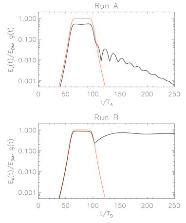
Figure 7: Time evolution of the electric field spectral component $E_{k}(t)$ (normalized by the maximum driver amplitude $E_{{}_{DM}}$) for Run A (top) and Run B (bottom); in both plots the red (gray) curve represents the function $g(t)$.

III Numerical simulations

Because the results of Sec. II are essentially linear in nature, we investigate their resilience by resorting to simulations of the nonlinear Vlasov-Poisson system of Eqs. (1). In particular, we concentrate on modes that arise from deviations of the thumb curve, off-dispersion modes, caused by the small plateaus.

Our simulations are performed with an Eulerian Vlasov code based on the well-know splitting time advance method given in Ref. knorr76 . The phase space domain for the simulations is $\mathcal{D}=[0,L]\times[-v_{{}_{max}},v_{{}_{max}}]$. Periodic boundary conditions in $x$ are assumed, while the electron velocity distribution is set equal to zero for $|v|>v_{{}_{max}}=6$. We investigate disturbances near the initial equilibrium of Eq. (3), with $n_{p}=10$ and $\Delta V_{p}=0.01$ by applying a drive force. The $x$-direction is discretized with $N_{x}=256$ grid points, while $v$-direction with $N_{v}=12000$. Our goal is to numerically analyze the modes predicted by Fig. 5.

The plasma is driven by an external electric field that is taken to be a sinusoidal traveling wave with phase speed $v_{\phi_{{}_{D}}}$ that exactly matches $V_{0}$, the location of the plateau of $f_{p}$. The explicit form of the external field is

$$E_{{}_{D}}(x,t)=g(t)E_{{}_{DM}}\sin{(kx-\omega_{{}_{D}}t)}\,,$$ (24)

where $E_{{}_{DM}}$ is the maximum driver amplitude, $k=2\pi/L$ is the drive wavenumber, which is the maximum wavelength that fits in the simulation box, $\omega_{{}_{D}}=kv_{\phi_{{}_{D}}}$ is the drive frequency, and $g(t)=[1+(t-\tau)^{n}/\Delta\tau^{n}]^{-1}$ is a profile that determines the ramping up and ramping down of the drive. The external electric field is applied directly to the electrons by adding $E_{{}_{D}}$ to $E$ in the Vlasov equation. An abrupt turn-on or turn-off of the drive field would excite LAN waves and complicate the results. Thus, we choose $n=10$ so $g(t)$ amounts to a nearly adiabatic turn-on and turn-off. The driver amplitude remains near $E_{{}_{DM}}$ for a time interval of order $\Delta\tau$ centered at $t=\tau$ and it is zero for $t\geq t_{\rm off}\simeq\tau+\Delta\tau/2$. We will analyze the plasma response for many wave periods after the driver has been turned off.

The effect of the driver is to prepare a state (i.e. distribution function), which is then used as an initial condition for the undriven Vlasov-Poisson system of Eqs. (1). This type of initial condition is an example of those called dynamically accessible in Morrison89 ; Morrison90 ; Morrison92 , where they were advocated and discussed in detail. Ultimately, any perturbation of a known distribution function within the confines of Vlasov-Poisson theory must, in fact, be caused by an electric field, since there are no other forces available. Thus it is physically very natural to consider such initial conditions. Dynamically accessible initial conditions are also important because they have a Hamiltonian origin and, consequently, preserve phase space constraints. Because the perturbed distribution function is obtained by evaluating the known state on particle orbits, the perturbed distribution function must have the same level set topology as the unperturbed and the areas between any level set contours must be preserved. For our simulations, the dynamically accessible initial conditions used amount to evaluating the plateau distribution of Eq. (3) on the orbits (run backwards) produced by the total electric field in the interval $0<t<t_{\rm off}$. Thus, the initial condition for the undriven dynamics that begins at $t_{\rm off}$ is a symplectic rearrangement of $f_{p}$ Morrison92 ; hagstrom ; Morrison12 .

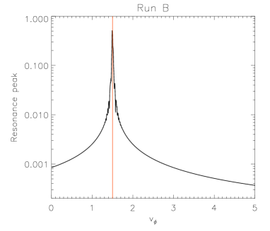
Figure 8: Resonance peak for Run B; red-vertical line indicates the value of the driver phase velocity $v_{\phi_{{}_{D}}}$.

We performed $N_{sim}=64$ simulations for various values of the plateau velocity position $V_{0}$ of $f_{p}$ and the wavenumber $k$, in order to numerically investigate the predictions of Fig. 5. For each simulation we chose $\Delta\tau=20T$, where $T=2\pi/kv_{\phi_{{}_{D}}}$ is the wave period (that is the plasma is driven for 20 wave periods) and $\tau=80T$. Typically the maximum time for the simulations is $t_{max}=250T$, but when needed the system evolution is followed up to $1000T$. The driver amplitude is set for each simulation by adjusting the driver trapping time $\tau_{trap}:=2\pi/\sqrt{kE_{{}_{DM}}}$ to be larger than $t_{max}$. In particular, we set $\tau_{trap}=125\Delta\tau=10t_{max}$, so that trapping does not play a large role in the system evolution, i.e. the distribution function changes little during the simulation.

Numerical results for $E$, show two different kinds of electric field response for $t>t_{\rm off}$. To see this we plot $E_{k}(t)$, the electric field $k$-spectral component, in the semi-log plots of Figs. 7, for two different runs denoted by A and B with parameters given in Table 1.

Run					$k$					$v_{\phi_{D}}$
A					0.9					0.3
B					0.7					1.5
C					0.4					1.561

Table 1: Relevant parameters for Runs A, B and C

In the plots of Figs. 7, the electric signals are normalized by the corresponding maximum driver amplitude $E_{{}_{DM}}$ and the red (gray) line represents the function $g(t)$. As is evident from the plots, in Run A we observe damped (more or less exponentially) oscillations after the driver has been turned off, consistent with Landau damping, while in Run B we observe a stable electric response, consistent with plateau suppression. Figure 8 is a semi-log plot of the spectral electrostatic energy, obtained by the Fourier analysis of $E$ for $t>t_{off}$, as a function of $v_{\phi}$, for the case of Run B, where a stable plasma response is recovered at $t>t_{off}$. This plot reveals that the electric field propagates with a phase velocity $v_{\phi}$ near the driver phase velocity $v_{\phi_{D}}$ (red-vertical line).

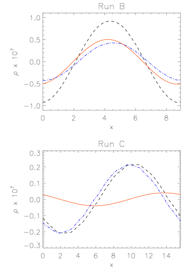
Figure 9: Spatial dependence of the electron charge densities $\rho$ (black-dashed line), $\rho_{1}$ (red-solid line), and $\rho_{2}$ (blue-dot-dashed line) for Run B (top) and Run C (bottom).

Moreover, for Run B we evaluated the electron charge density $\rho=1-\int fdv$ at the end of the simulation. This undamped mode with the parameters of Table 1 is located off of the thumb curve (see Fig. 1). The black-dashed line in the top plot of Fig 9 is the total electron charge density, $\rho$, obtained by integrating $f$ over the velocity interval $I=[-v_{{}_{max}},v_{{}_{max}}]$, the red-solid line is the charge density, $\rho_{1}$, obtained by integrating $f$ over the velocity interval $I_{v}=[1.48,1.52]$ near $V_{0}$, while the blue-dot-dashed line is the charge density, $\rho_{2}$, obtained by integrating over the complement of $I_{v}$. Clearly, $\rho=\rho_{1}+\rho_{2}$. From the plot it is seen that the contribution to the charge density coming from the small interval $I_{v}$ around $V_{0}$, which contains the sharp corners at the boundaries of the plateau, is comparable to or even a bit larger than the contribution from the rest of the velocity distribution. The same calculation has also been performed for a third Run C, whose parameters are summarized in table 1. This mode falls on the thumb curve. Here, as can be seen in the bottom plot of Fig. 9, the contribution to the charge density from the sharp corners within the interval $I_{v}$ around $V_{0}$ (red-solid line) is significantly smaller than that of the rest of the velocity distribution. These runs provide numerical evidence that supports the predictions of Sec. II for the perturbed distribution function summarized in Fig. 6.

In order to reproduce numerically the predictions displayed in Fig. 5, we analyzed in detail the results of $N_{sim}=64$ numerical experiments. For each simulation we evaluated the real part of the frequency $\omega_{{}_{R}}$ and the wave damping rate $\omega_{{}_{I}}$ after the external driver was turned off. Each simulation is then characterized by calculating $|\omega_{{}_{I}}/\omega_{{}_{R}}|:=R$ from the simulation data. To compare the simulation results with the contour plot of Fig. 5, we use the value $R_{th}^{{}^{max}}$ from Sec. II as a threshold to divide our 64 simulations into two classes: Class $1$ for which $R\leq R_{th}^{{}^{max}}$ and Class $2$ for which $R>R_{th}^{{}^{max}}$.

These results are summarized in the $k-V_{0}$ scatter plot of Fig. 10, where the simulations of Class $1$ are indicated by black squares, while those of Class $2$ by red diamonds. In this figure the red-dashed line indicates as usual the thumb curve, while the black-solid lines delimits the dark region of the contour plot in Fig. 5, where almost undamped roots of the dielectric function have been recovered. Figure 10 clearly shows that the black squares fall within the black-solid line, while the red diamonds lie outside this line; thus, results of the analysis of Fig. 5 are well corroborated by the simulations. The simulations of runs Run A, Run B, and Run C are indicated by capital letters in Fig. 10. Runs A fall outside the black-solid lines, Runs B fall inside the dark region with black solid-line boundaries, and Runs C are exactly on the thumb curve indicated by the red-dashed line.

IV Summary and conclusions

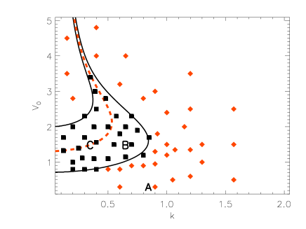
Figure 10: $k-V_{0}$ scatter plot for Class 1 simulations (black squares) and Class 2 simulations (red diamonds). The red-dashed line is the thumb curve, while the black curves delimit the dark region of the contour plot of Fig. 5.

In the present work, roots of the electrostatic dielectric function were analyzed when a velocity plateau of small but nonvanishing width is present in the equilibrium velocity distribution of electrons. The numerical solution of the Landau integral, performed through a high resolution scheme, allowed us to show that quasi-undamped plasma oscillations can be obtained off of the thumb curve of Ref. holloway91 . By solving numerically the Landau integral, we noted that the presence of the velocity plateau, even of very small width, can highly affect the real part of the dielectric function, producing marked spikes within the velocity interval around the plateau. In a wide region of the $k-\omega_{{}_{R}}$ plane, almost undamped roots of the dielectric function were obtained. Examination of the perturbed electron distribution function revealed that most of the charge density associated with the off-dispersion oscillations comes from the sharp corners at the boundaries of the velocity plateau, and for this reason we called these new modes corner modes. A rule of thumb was derived by assuming infinitely sharp corners, a rule useful for gauging how a plateau shifts roots off of the thumb curve.

Next, these analytical predictions were compared with the results of Eulerian Vlasov-Poisson simulations with high resolution in velocity space. Our simulations were initiated by applying a wave-like external electric field to drive the plateau distribution of Eq. (3) off of equilibrium. The external electric field was turned on and off adiabatically in such a way to avoid the excitation of usual Langmuir waves. Also, the amplitude of the external driver was chosen to be very small so trapping effects were minimized. As discussed in Sec. III, the numerical results of these nonlinear simulations corroborated the linear results of Sec. II.

Although we spoke of off-dispersion results, it is important to note that all of the roots obtained in Sec. II are actual linear electrostatic plasma oscillations: while LAN waves are approximate time asymptotic states as shown by Landau; EAWs, corner modes, stationary inflection point modes, etc. are all exact linear plasma oscillations for specific homogeneous equilibrium distribution functions. In essence, what we are really attempting is to find a homogeneous equilibrium distribution function that best describes a weakly nonlinear theory. Because plasmas can exist in states away from thermodynamic equilibrium for substantial lengths of time, there is no a priori reason to believe the distribution function is Maxwellian, particularly if wave-like disturbances are excited. Because of the sensitivity of the dispersion relation to equilibrium distribution functions, in the tail but particularly near $v_{\phi}$, we conclude that the thumb curve of Ref. holloway91 is of limited predictive capability.

Since the original BGK paper bernstein57 , it has been understood that there is nonuniqueness in the construction of these nonlinear modes: a given electric field can be consistent with a large class of distribution functions. It is difficult to pin down the shape of the distribution function for the trapped particle population, because the formation of this distribution depends on the time history. This is true both in experiments and simulations, whether the BGK modes evolve out of instability or arise by driving the plasma as we have done here. In the case of small amplitude disturbances, we make the point that this arbitrariness is the same as that in choosing the appropriate shape of $f_{0}(v)$ near $v_{\phi}$. For very small disturbances, the stationary inflection point modes of shadwick94 are natural candidates. For larger disturbances, the off-dispersion modes of this paper appear to be an attractive alternative.

Thus, the present work bears on the interpretation of recent results of nonneutral plasma experiments that provide evidence for undamped off-dispersion modes. In the experiments of anderegg091 ; anderegg092 , any plateau-like structures in the electron velocity distribution are created dynamically by means of an external driver electric field that traps resonant particles. After the driving process, the plasma is strongly inhomogeneous, with the formation of humps and depressions in the particle distribution function, produced by the nonlinear dynamics triggered by the external field. Thus, one would think that a linear analysis might not be relevant; however, by designing a plateau and tail for a distribution function that has modes that match the experiment, it appears that one can obtain a linear theory consistent with some of the experimental results, and possibly even infer information about the trapped particles. In fact, we note that the rule of thumb explains the frequency shifts observed in the experiments of anderegg092 , but continuing with this line of investigation is beyond the scope of the present paper, so we conclude here.

References

- (1) L. D. Landau, J. Phys. (Moscow) 10, 25 (1946).
- (2) T. M. O’Neil, Phys. Fluids 8, 2255 (1965).
- (3) J. P. Holloway and J. J. Dorning, Phys. Rev. A 44, 3856 (1991).
- (4) I. B. Bernstein, J. M. Greene and M. D. Kruskal, Phys. Rev. 108, 546 (1957).
- (5) L. Demeio and J. P. Holloway, J. Plasma Phys. 46, 63 (1991).
- (6) B. A. Shadwick and P. J. Morrison, Phys. Lett. A 184, 277 (1994).
- (7) G. I. Hagstrom and P. J. Morrison, Transport Theory Stat. Phys. 39, 466 (2011).
- (8) F. Valentini, T. M. O’Neil and D. H. Dubin, Phys. Plasmas 13, 052303 (2006).
- (9) B. Afeyan, K. Won, V. Savchenko, T. W. Johnston, A. Ghizzon, and P Bertrand, “Kinetic Electrostatic Electron Nonlinear (KEEN) Waves and their Interactions Driven by the Ponderomotive Force of Crossing Laser Beams,” Proc. Inertial Fusion Sciences and Applications 2003 (B. Hamel, D. D. Meyerhofer, J. Meyer-ter-Vehn, and H. Azechi, Eds.), Monterey: American Nuclear Society (2004) p. 213B.
- (10) T. W. Johnston, Y. Tyshetskiy, A. Ghizzo and P. Bertrand, Phys. Plasmas 16, 042105 (2009).
- (11) F. Valentini, F. Califano, D. Perrone, F. Pegoraro and P. Veltri, Phys. Rev. Lett. 106, 165002 (2011).
- (12) F. Valentini, F. Califano, D. Perrone, F. Pegoraro and P. Veltri, Plasma Phyc. Control. Fusion 53, 105017 (2011).
- (13) S. P. Gary and R. L. Tokar, Phys. Fluids 28, 2439 (1985).
- (14) F. Anderegg, C. F. Driscoll, D. H. Dubin, T. M. O’Neil, Phys. Rev. Lett. 102, 09500 (2009).
- (15) F. Anderegg, C. F. Driscoll, D. H. Dubin, T. M. O’Neil and F. Valentini, Phys. Plasmas 16, 055705 (2009).
- (16) S. Montgomery, J. A. Cobble, J. C. Fern ndez, R. J. Focia, R. P. Johnson, N. Renard-LeGalloudec, H. A. Rose, and D. A. Russell, Phys. Plasmas 9, 2311 (2002).
- (17) T. M. O’Neil and J. H. Malmberg, Phys. Fluids 11, 1754 (1968).
- (18) N. A. Krall and A. W. Trivelpiece, Principles of Plasma Physics, (San Francisco Press, San Francisco, CA, 1986).
- (19) M. Abramowitz and I. Stegun, (1972), Handbook of Mathematical Functions, (Dover Publications, New York, 1972), item 7.1.13 p. 298.
- (20) C. Z. Cheng and G. Knorr, J. Comp. Phys. 22, 330 (1976).
- (21) P. J. Morrison and D. Pfirsch, Phys. Rev. A 40, 3898 (1989).
- (22) P. J. Morrison and D. Pfirsch, Phys. Fluids B 2, 1105 (1990).
- (23) P. J. Morrison and D. Pfirsch, Phys. Fluids B 4, 3038 (1992).
- (24) P. J. Morrison, Math-for-Industry 39, 64 (2012).