Trace formula for dielectric cavities III: TE modes

Abstract

The construction of the semiclassical trace formula for the resonances with the transverse electric (TE) polarization for two-dimensional dielectric cavities is discussed. Special attention is given to the derivation of the two first terms of Weyl’s series for the average number of such resonances. The obtained formulas agree well with numerical calculations for dielectric cavities of different shapes.

I Introduction

Open dielectric cavities have attracted a large interest in recent years due to their numerous and potentially important applications vahala ; matsko . From a theoretical point of view, the crucial difference between dielectric cavities and much more investigated case of closed quantum billiards balian_bloch ; gutzwiller ; haake is that in the latter the spectrum is discrete but in the former it is continuous. Indeed, the main subject of investigations in open systems is not the true spectrum but the spectrum of resonances defined as poles of the scattering $S$-matrix (see e.g. scattering ; s_matrix ).

The wavelength of electromagnetic field is usually much smaller than any characteristic cavity size (except its height) and semiclassical techniques are useful and adequate for a theoretical approach to such objects. It is well known that the trace formulas are a very powerful tool in the semiclassical description of closed systems, see e.g. balian_bloch ; gutzwiller ; haake . Therefore, the generalization of trace formulas to different open systems, in particular to dielectric cavities, is of importance.

The trace formula for resonances with transverse magnetic (TM) polarization in two-dimensional (2d) dielectric cavities has been developed in trace1 and shown to agree well with the experiments and numerical calculations trace2 ; stefan2010-2012 .

This paper is devoted to the construction of the trace formula for 2d dielectric cavities but for transverse electric (TE) polarization. Due to different boundary conditions the case of TE modes differs in many aspects from TM modes. In particular, a special treatment is required for the resonances related to Brewster’s angle jackson at which the Fresnel reflection coefficient vanishes.

Our main result is the asymptotic formula in the semiclassical (aka short wave length) regime for the average number of TE resonances for a 2d dielectric cavity with refraction index $n$, area $\mathcal{A}$ and perimeter $\mathcal{L}$

$$\bar{N}_{\mathrm{TE}}(k)=\frac{\mathcal{A}\,n^{2}k^{2}}{4\pi}+r_{\mathrm{TE}}(n)\frac{\mathcal{L}\,k}{4\pi}+o(k)\ .$$ (1)

Here $\bar{N}_{\mathrm{TE}}(k)$ is the mean number of resonances (defined below) whose real part is less than $k$, the coefficient $r_{\mathrm{TE}}$ is given by the expression

$$r_{\mathrm{TE}}(n) = 1+\frac{1}{\pi}\int_{-\infty}^{\infty}\tilde{R}_{\mathrm{TE}}(t)\left(\frac{n^{2}}{n^{2}+t^{2}}-\frac{1}{1+t^{2}}\right)\mathrm{d}t$$ (2)

$$+ \frac{2n}{\sqrt{n^{2}+1}}\ ,$$

and $\tilde{R}_{\mathrm{TE}}$ is the Fresnel reflection coefficient for the scattering on a straight dielectric interface at imaginary momentum

$$\tilde{R}_{\mathrm{TE}}(t)=\frac{\sqrt{n^{2}+t^{2}}-n^{2}\sqrt{1+t^{2}}}{\sqrt{n^{2}+t^{2}}+n^{2}\sqrt{1+t^{2}}}\ .$$ (3)

The plan of the paper is the following. In Sec. II the main equations describing the TE modes are reminded. In Sec. III the circular cavity is briefly reviewed: an exact quantization condition is derived, which allows a direct semiclassical treatment. In Sec. IV the first two Weyl terms for the resonance counting function are derived. It is important to notice that, for TE modes, one can have total transmission of a ray when the incidence angle is equal to Brewster’s angle. This leads to a special set of resonances, which are counted separately in Sec. V. Section VI is devoted to a brief derivation of the oscillating part of the resonance density. In Sec. VII our obtained formulae are shown to agree well with numerical computation for cavities of different shapes. In Appendix A another method of deriving the Weyl series for TE polarization based on Krein’s spectral shift formula is presented.

II Generalities

To describe a dielectric cavity correctly one should solve the $3$-dimensional Maxwell equations. In many applications the transverse height of a cavity, say along the $z$ axis, is much smaller than any other cavity dimensions. In such situation the $3$-dimensional problem in a reasonable approximation can be reduced to two 2d scalar problems (for each polarization of the field) following the so-called effective index approximation, see e.g. melanie2007 ; melanie2008 for more details.

In the simplest setting, when one ignores the dependence of the effective index on frequency, such 2d approximation consists in using the Maxwell equations for an infinite cylinder. It is well known jackson that in this geometry the Maxwell equations are reduced to two scalar Helmholtz equations inside and outside the cavity

$$(\Delta+n^{2}k^{2})\Psi(\vec{x}\,)=0, \vec{x}\in{\cal D}\ ,$$

$$(\Delta+k^{2})\Psi(\vec{x}\,)=0, \vec{x}\notin{\cal D}\ ,$$ (4)

where $n$ is the refractive index of the cavity, ${\cal D}$ indicates the interior of the dielectric cavity, and $\Psi=E_{z}$ for the TM polarization and $\Psi=B_{z}$ for the TE polarization.

Helmholtz equations (4) have to be completed by the boundary conditions. The field, $\Psi(\vec{x}\,)$, is continuous across the cavity boundary and its normal derivatives along both sides of the boundary are related for two polarizations as below jackson

$$\frac{\partial\Psi}{\partial\nu}|_{\mathrm{from\;inside}}=\left\{\begin{array}[]{cc}\dfrac{\partial\Psi}{\partial\nu}|_{\mathrm{from\;outside}},&\mathrm{for\;TM}\ ,\\ \\ n^{2}\dfrac{\partial\Psi}{\partial\nu}|_{\mathrm{from\;outside}},&\mathrm{for\;TE}\ .\end{array}\right.$$ (5)

Open cavities have no true discrete spectrum. Instead, we are interested in the discrete resonance spectrum, which is defined as the (complex) poles of the $S$-matrix for the scattering on a cavity (see e.g. s_matrix ). It is well known that the positions of the resonances can be determined directly by the solution of the problem (4) and (5) by imposing the outgoing boundary conditions at infinity

$$\Psi(\vec{x})\propto e^{\mathrm{i}k|\vec{x}|}\quad|\vec{x}|\to\infty\ .$$ (6)

The set (4)-(6) admit complex eigen-values $k$ with Im$\ k<0$, which are the resonances of the dielectric cavity and are the main object of this paper. Our goal is to count such resonances for the TE polarization in the semiclassical regime. This will provide us with the analogue of Weyl’s law derived for closed systems, see e.g. baltes .

III Circular cavity

The circular dielectric cavity is the only finite 2d cavity, which permits an analytical solution. Let $R$ be the radius of such a cavity. Writing $\Psi(\vec{x}\,)=AJ_{m}(nkr)\mathrm{e}^{\mathrm{i}m\phi}$ inside the cavity and $\Psi(\vec{x}\,)=BH_{m}^{(1)}(kr)\mathrm{e}^{\mathrm{i}m\phi}$ outside the cavity, it is plain to check, that in order to fulfill the boundary conditions, it is necessary that $k$ is determined from the equation $s_{m}(x)=0$ with $x=kR$ and

$$s_{m}(x)=x\Big{[}\frac{1}{n}J_{m}^{\prime}(nx)H_{m}^{(1)}(x)-J_{m}(nx)H_{m}^{(1)\,\prime}(x)\Big{]}$$ (7)

where $J_{m}(x)$ (resp. $H_{m}^{(1)}(x)$) denotes the Bessel function (resp. the Hankel function of the first kind). Here and below the prime indicates the derivative with respect to the argument. Factor $x$ in (7) is introduced for further convenience.

Using $J_{m}(x)=(H_{m}^{(1)}(x)+H_{m}^{(2)})/2$ the equation $s_{m}(x)=0$ can be rewritten in the form

$$R_{m}(x)E_{m}(x)=1\ ,$$ (8)

where

$$E_{m}(x)=\frac{H_{m}^{(1)}}{H_{m}^{(2)}}(nx)$$ (9)

and

$$R_{m}(x)=\dfrac{\frac{H_{m}^{(1)\,\prime}}{H_{m}^{(1)}}(nx)-n\frac{H_{m}^{(1)\,\prime}}{H_{m}^{(1)}}(x)}{-\frac{H_{m}^{(2)\,\prime}}{H_{m}^{(2)}}(nx)+n\frac{H_{m}^{(1)\,\prime}}{H_{m}^{(1)}}(x)}\ .$$ (10)

In the semiclassical limit, $x\to\infty$, the asymptotic formula for the Hankel function bateman ($0\leq m\leq x$) gives

$$H_{m}^{(1)}(x)\simeq\frac{\sqrt{2/\pi}}{(x^{2}-m^{2})^{1/4}}\mathrm{e}^{\mathrm{i}\Phi_{m}(x)}\left[1+\mathcal{O}(x^{-1})\right]$$ (11)

where

$$\Phi_{m}(x)=\sqrt{x^{2}-m^{2}}-m\arccos\left(\frac{m}{x}\right)-\frac{\pi}{4}\ .$$ (12)

In this way one obtains

$$E_{m}\underset{x\to\infty}{\longrightarrow}\mathrm{e}^{2\mathrm{i}\Phi_{m}(nx)}$$ (13)

and

$$R_{m}(x)\underset{x\to\infty}{\longrightarrow}R_{\mathrm{TE}}\left(\frac{m}{x}\right)$$ (14)

where $R_{\mathrm{TE}}$ is the standard TE Fresnel coefficient for the scattering on an infinite dielectric interface

$$R_{\mathrm{TE}}(t)=\frac{\sqrt{n^{2}-t^{2}}-n^{2}\sqrt{1-t^{2}}}{\sqrt{n^{2}-t^{2}}+n^{2}\sqrt{1-t^{2}}}\ .$$ (15)

The above formulas mean that in the semiclassical limit, Eq. (8) takes the form

$$R_{\mathrm{TE}}\left(\frac{m}{x}\right)\mathrm{e}^{2\mathrm{i}\Phi_{m}(nx)}=1$$ (16)

or

$$\Phi_{m}(nx)=\pi p+\frac{\mathrm{i}}{2}\ln R_{\mathrm{TE}}\left(\frac{m}{x}\right)$$ (17)

with integer $p=0,1,2,\ldots$.

In fact, this equation is valid in the semiclassical limit for closed and open circular cavities with other boundary conditions as well. The only difference is that, instead of the Fresnel reflection coefficient $R_{\mathrm{TE}}$, it is necessary to use the reflection coefficient for the problem under consideration. For example, for closed billiards, $n=1$ and for Neumann (resp. Dirichlet) boundary conditions $R_{m}(x)$ in (14) equals to $1$ (resp. $-1$). For open dielectric circular cavity with the TM polarization $R_{m}(x)\to R_{\mathrm{TM}}\left(m/x\right)$, where $R_{\mathrm{TM}}$ is the usual Fresnel reflection coefficient for the TM modes jackson

$$R_{\mathrm{TM}}(t)=\frac{\sqrt{n^{2}-t^{2}}-\sqrt{1-t^{2}}}{\sqrt{n^{2}-t^{2}}+\sqrt{1-t^{2}}}\ .$$ (18)

IV Weyl terms

Semiclassical formulas like Eq. (16) are convenient to obtain the average number of eigenvalues and resonances for closed and open systems with different boundary conditions.

Let us consider first the simplest case of a closed billiard with Neumann boundary conditions for which $R_{m}(x)=1$. In the semiclassical regime the eigenvalues for this model are determined from Eq. (17) which reads

$$\Phi_{m}(x)=\pi p\ ,$$ (19)

where $\Phi_{m}(x)$ is defined in (12) and $p=0,1,\ldots$ is an integer. Therefore, for fixed $m$, the number of eigenvalues less than $x$ is $[N_{m}(x)]$ where $[\;.\;]$ stands for the integer part and

$$N_{m}(x)=\frac{1}{\pi}\Phi_{m}(x)+1\ .$$ (20)

$1$ is added as the integer $p$ in (19) starts with $0$ but $[N_{m}(x)]$ has to begin with $1$.

Summing over all $m$ leads to the total number of eigenvalues less than $x$, usually called the counting function. This sum is finite as the asymptotics (11) is valid when $|m|\leq x$. Finally

$$N(x)=\sum_{m=-|x|}^{[x]}\Big{[}N_{m}(x)\Big{]}\ .$$ (21)

The averaged number of levels is determined from the equation

$$\bar{N}(x)=\sum_{m=-x}^{x}\left(N_{m}(x)-\tfrac{1}{2}\right)\ .$$ (22)

With a needed precision one can substitute the summation over $m$ by an integral and, consequently, the averaged number of eigenvalues for a circular billiard with Neumann boundary conditions can be approximated as follows

$$\bar{N}(x)=2\int_{0}^{x}\Big{(}\frac{1}{\pi}(\sqrt{x^{2}-m^{2}}-m\arccos\left(\frac{m}{x}\right))+\frac{1}{4}\Big{)}\mathrm{d}m\ .$$ (23)

Using the formula

$$\int_{0}^{1}(\sqrt{1-t^{2}}-t\arccos(t))\mathrm{d}t=\frac{\pi}{8}$$ (24)

one gets

$$\bar{N}(x)=\frac{1}{4}x^{2}+\frac{1}{2}x+\mathcal{O}(1)\ .$$ (25)

As for the circle the area is $\mathcal{A}=\pi R^{2}$ and the perimeter is $\mathcal{L}=2\pi R$, these results can be rewritten in the standard form baltes

$$\bar{N}(k)=\frac{\mathcal{A}\,k^{2}}{4\pi}+r\frac{\mathcal{L}\,k}{4\pi}+\mathcal{O}(1)\$$ (26)

with $r=1$. For Dirichlet boundary conditions similar arguments show that $1/4$ in (23) is substituted by $-1/4$ and $r=-1$, as it should be baltes .

For open cavities Eq. (16) gives complex solutions (resonances) $k=k_{1}+\mathrm{i}k_{2}$ with negative imaginary part, $k_{2}<0$. In the semiclassical limit for all investigated cases one has $|k_{2}|\ll k_{1}$. Separating the imaginary and real parts in (17) and using that

$$\frac{\partial}{\partial x}\Phi_{m}(x)=\sqrt{1-\frac{m^{2}}{x^{2}}}$$ (27)

one gets that in the first order in $k_{2}$ the real part of the resonance position, $k_{1}$ (or $x_{1}=k_{1}R$), is determined from the real equation similar to (17)

$$\Phi_{m}(nx_{1})+\delta(m/x_{1})=\pi p,\quad p\textrm{ integer},$$ (28)

where $2\delta(t)$ is the argument of the reflection coefficient

$$R(t)=|R(t)|\mathrm{e}^{2\mathrm{i}\delta(t)}\ .$$ (29)

In the same approximation the imaginary part of the resonance position, $k_{2}$ is

$$k_{2}R=\frac{\ln|R(x_{1})|}{2\sqrt{n^{2}-m^{2}/x_{1}^{2}}}\ .$$ (30)

This semiclassical approximation is quite good even for not too large $m$ as indicated in Fig. 1.

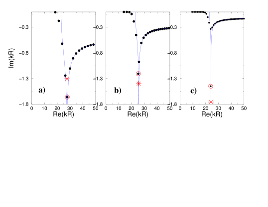
Figure 1: (Color online). The black circles are the exact positions of the resonances with $m=23$ and $n=1.5$ (a), $n=2$ (b), and $n=3$ (c). The blue lines indicate the approximation (30). The additional levels are encircled by the red circles. The red stars show the approximate formula (48).

The above arguments demonstrate that the total number of resonances can be calculated from the real equation (28). As in (22) one concludes that the mean number of resonances with real part $x_{1}$ less than $x$ is given by the expression

$$\bar{N}(x)=\sum_{m=-nx}^{nx}\left(N_{m}(x)-\tfrac{1}{2}\right)$$ (31)

with

$$N_{m}(x)=\frac{1}{\pi}\Phi_{m}(nx)+\frac{1}{\pi}\delta\left(\frac{m}{x}\right)+1\ .$$ (32)

Consider first the case of TM modes. The reflection coefficient in this case is given by (18) and one has

$$\delta_{\mathrm{TM}}(t)=\left\{\begin{array}[]{rr}-\arctan\left(\dfrac{\sqrt{t^{2}-1}}{\sqrt{n^{2}-t^{2}}}\right),&1\leq t\leq n\\ \\ 0,&0\leq t\leq 1\end{array}\right.\ .$$ (33)

Therefore

$$\bar{N}(x) = 2\int_{0}^{nx}\frac{1}{\pi}\left[\sqrt{n^{2}x^{2}-m^{2}}-m\arccos\left(\frac{m}{nx}\right)\right]\mathrm{d}m$$ (34)

$$+ 2\int_{0}^{nx}\left[\frac{1}{\pi}\delta_{\mathrm{TM}}\left(\frac{m}{x}\right)+\frac{1}{4}\right]\mathrm{d}m=\frac{n^{2}}{4}x^{2}+\frac{n}{2}x$$

$$- \frac{2x}{\pi}\int_{1}^{n}\arctan\left(\frac{\sqrt{t^{2}-1}}{\sqrt{n^{2}-t^{2}}}\right)\mathrm{d}t\ .$$

By integration by parts and contour deformation it is easy to check that

$$2\int_{1}^{n}\arctan\left(\frac{\sqrt{t^{2}-1}}{\sqrt{n^{2}-t^{2}}}\right)\mathrm{d}t=\frac{\pi}{2}(n-1)$$ (35)

$$- \int_{0}^{\infty}\tilde{R}_{\mathrm{TM}}(t)\left(\frac{n^{2}}{n^{2}+t^{2}}-\frac{1}{1+t^{2}}\right)\mathrm{d}t$$

where $\tilde{R}_{\mathrm{TM}}(t)$ is the same as (18) but for pure imaginary argument

$$\tilde{R}_{\mathrm{TM}}(t)\equiv{R}_{\mathrm{TM}}(\mathrm{i}t)=\frac{\sqrt{n^{2}+t^{2}}-\sqrt{1+t^{2}}}{\sqrt{n^{2}+t^{2}}+\sqrt{1+t^{2}}}\ .$$ (36)

Finally, these considerations lead to the expression similar to (26)

$$\bar{N}_{\mathrm{TM}}(k)=\frac{\mathcal{A}\,n^{2}k^{2}}{4\pi}+r_{TM}\frac{\mathcal{L}\,k}{4\pi}+o(k)$$ (37)

where

$$r_{TM}(n)=1+\frac{1}{\pi}\int_{-\infty}^{\infty}\tilde{R}_{\mathrm{TM}}(t)\left(\frac{n^{2}}{n^{2}+t^{2}}-\frac{1}{1+t^{2}}\right)\mathrm{d}t$$ (38)

which agrees with the result in trace1 obtained by a different method.

Consider now TE modes. In this case the reflection coefficient is given by (15) and its argument is

$$\delta_{\mathrm{TE}}(t)=\left\{\begin{array}[]{rr}-\arctan\left(\dfrac{n^{2}\sqrt{t^{2}-1}}{\sqrt{n^{2}-t^{2}}}\right),&1\leq t\leq n\\ \\ 0,&t^{*}\leq t\leq 1\\ \\ -\dfrac{\pi}{2},&0\leq t\leq t^{*}\end{array}\right.$$ (39)

where $t^{*}$ corresponds to the zero of the TE reflection coefficient (Brewster’s angle), $R_{\mathrm{TE}}(t^{*})=0$,

$$t^{*}=\frac{n}{\sqrt{n^{2}+1}}\ .$$ (40)

Using these values we get

$$\bar{N}_{\mathrm{TE}}(k)=\frac{\mathcal{A}\,n^{2}k^{2}}{4\pi}+r_{TE}\frac{\mathcal{L}\,k}{4\pi}+o(k)\$$ (41)

where $r_{TE}$ is given by the following expression

$$r_{TE}(n) = -\frac{4}{\pi}\int_{1}^{n}\arctan\left(\frac{n^{2}\sqrt{t^{2}-1}}{\sqrt{n^{2}-t^{2}}}\right)\mathrm{d}t$$ (42)

$$+ n-2\int_{0}^{t^{*}}\mathrm{d}t\ .$$

Similar to (35) one can prove that

$$2\int_{1}^{n}\arctan\left(n^{2}\frac{\sqrt{t^{2}-1}}{\sqrt{n^{2}-t^{2}}}\right)\mathrm{d}t=\frac{\pi}{2}(n-1)$$ (43)

$$- \int_{0}^{\infty}\tilde{R}_{\mathrm{TE}}(t)\left(\frac{n^{2}}{n^{2}+t^{2}}-\frac{1}{1+t^{2}}\right)\mathrm{d}t$$

where, as above, $\tilde{R}_{\mathrm{TE}}(t)$ is the TE reflection coefficient (15) analytically continued to imaginary $t$

$$\tilde{R}_{\mathrm{TE}}(t)\equiv R_{\mathrm{TE}}(\mathrm{i}t)=\frac{\sqrt{n^{2}+t^{2}}-n^{2}\sqrt{1+t^{2}}}{\sqrt{n^{2}+t^{2}}+n^{2}\sqrt{1+t^{2}}}\ .$$ (44)

Combining all terms together we obtain that

$$r_{TE}(n) = 1+\frac{1}{\pi}\int_{-\infty}^{\infty}\tilde{R}_{\mathrm{TE}}(t)\left(\frac{n^{2}}{n^{2}+t^{2}}-\frac{1}{1+t^{2}}\right)\mathrm{d}t$$ (45)

$$- \frac{2n}{\sqrt{n^{2}+1}}\ .$$

The first two terms are the same as for TM modes (38) but with TE reflection coefficient. The last term is the new one related to the change of the sign of the TE reflection coefficient.

Higher order terms in Weyl’s expansions (37) and (41) are not yet calculated so we prefer to use a conservative estimate of them as $o(k)$ though all numerical checks suggest that for smooth boundary cavities it is $\mathcal{O}(1)$.

V Additional resonances

Formula (45) is the correct description for the resonances whose real part of the eigen-momentum $k$ corresponds to non-zero reflection coefficient (i.e. $m/x_{1}\neq t^{*}$). This is due to the fact that when the reflection coefficient is zero its phase is not defined. For TE modes there is a special branch of resonances for which semiclassically the real part does obey $m/x_{1}=t^{*}$. The existence of such additional resonances were first discussed in a different context in sieber .

The approximate positions of these resonances can be calculated as follows. Assume that the resonances have a large imaginary part. As $H_{m}^{(2)}(x-\mathrm{i}\tau)$ tends to zero when $\tau\to\infty$ one can approximate Eq. (7) by

$$\tilde{s}_{m}(x)=0,\quad\tilde{s}_{m}(x)=\frac{H_{m}^{(1)\,\prime}}{H_{m}^{(1)}}(nx)-n\frac{H_{m}^{(1)\,\prime}}{H_{m}^{(1)}}(x)\ .$$ (46)

From the asymptotic (11) it follows that

$$\frac{H_{m}^{(1)\,\prime}}{H_{m}^{(1)}}(x)\underset{x\to\infty}{\longrightarrow}\mathrm{i}\sqrt{1-\frac{m^{2}}{x^{2}}}-\frac{x}{2(x^{2}-m^{2})}\ .$$ (47)

Using this expression one concludes that the solution of the equation $\tilde{s}_{m}(\tilde{x}_{m})=0$ has the form

$$\tilde{x}_{m}\approx\frac{\sqrt{n^{2}+1}}{n}m-\mathrm{i}\frac{(n^{2}+1)^{3/2}}{2n^{2}}\ .$$ (48)

This approximation is better for large $n$ when the imaginary part is large but it gives reasonable results even for $n$ of the order of $1$. In practice one may use (48) as the initial value for any root search algorithm (cf. Fig. 1).

From (48) it follows that the ratio $m/\tilde{x}_{m}$ tends to $t^{*}$ defined in (40) so these resonances are not taken explicitly into account in Eq. (45). Their number can be estimated as follows. The discussed resonances correspond to waves propagating along the boundary whose direction forms an angle with the normal exactly equal to Brewster’s angle

$$\sin\theta_{\mathrm{B}}=\frac{n}{\sqrt{n^{2}+1}}$$ (49)

If the length of the boundary is $\mathcal{L}$, the possible values for the momenta of such states in the semiclassical limit are

$$k_{m}\sin\theta_{\mathrm{B}}=\frac{2\pi}{\mathcal{L}}m$$ (50)

with integer $m=0,\pm 1,\pm 2,\ldots$. Therefore, the number of additional resonances related with Brewster’s angle is

$$N_{\mathrm{add}}(k)\approx\frac{\mathcal{L}\,k}{\pi}\frac{n}{\sqrt{n^{2}+1}}\ .$$ (51)

Comparing it with Eq. (45) we conclude that the second term in the Weyl expansion for the averaged number of resonances for TE polarization is the following

$$r_{TE} = 1+\frac{1}{\pi}\int_{-\infty}^{\infty}\tilde{R}_{\mathrm{TE}}(t)\left(\frac{n^{2}}{n^{2}+t^{2}}-\frac{1}{1+t^{2}}\right)\mathrm{d}t$$ (52)

$$\pm \frac{2n}{\sqrt{n^{2}+1}}$$

where the plus sign is used when the above additional resonances are taken into account and the minus sign corresponds to the case when these resonances are ignored.

For small values of $n$ the additional resonances are mixed with other resonances and their separation seems artificial. For large $n$ the additional branch of resonances is well separated from the main body of resonances and one can decide not to take them into account. In such a case, the minus sign has to be used in (52) (see below Section VII).

When the cavity remains invariant under a group of symmetry it is often convenient to split resonances according to their symmetry representations. For reflection symmetries it is equivalent to consider a smaller cavity where along parts of the boundary one has to impose either Dirichlet or Neumann boundary conditions. In this case the total boundary contribution to the average counting function $\bar{N}(k)$ is given by the general formula

$$\frac{1}{4\pi}\left(n(L_{N}-L_{D})+r_{TE}(n)L_{0}\right)k\ .$$ (53)

Here $L_{N}$ and $L_{D}$ are the lengths of the boundary parts with respectively Neumann and Dirichlet boundary conditions and $L_{0}$ is the length of the true dielectric interface. It is this formula, which will be used in Section VII for dielectric cavities in the shape of a square and a stadium.

VI Oscillating part of the trace formula

The quantization conditions (7) or (8) permit also to obtain the resonance trace formula for a circular dielectric cavity. Let $k_{j}=k_{1j}-\mathrm{i}k_{2j}$ be resonance eigen-momenta. Define the density of resonances as follows

$$d(k)=-\frac{1}{\pi}\mathrm{Im}\,\sum_{j}\frac{1}{k-k_{j}}=\frac{1}{\pi}\sum_{j}\frac{k_{2j}}{(k-k_{1j})^{2}+k_{2j}^{2}}\ .$$ (54)

In general, if $x_{j}$ are the zeros of a certain function $F(x)$ which has no other singularities then the density of these zeros (54) formally is given by the following expression

$$d(x)=-\frac{1}{\pi}\mathrm{Im}\frac{F^{\prime}(x)}{F(x)}\ .$$ (55)

In the semiclassical limit $k\to\infty$ it is sufficient to consider the semiclassical formula (16) i.e. $F(x)=\prod_{m}F_{m}(x)$ and

$$F_{m}(x)=1-R_{\mathrm{TE}}\left(\frac{m}{x}\right)\mathrm{e}^{2\mathrm{i}\Phi_{m}(nx)}\ .$$ (56)

A more careful discussion is performed in Appendix A. In such a manner one gets

$$d^{(osc)}(k)=\frac{2R}{\pi}\sum_{m=-\infty}^{\infty}\mathrm{Re}\,\sqrt{n^{2}-\frac{m^{2}}{x^{2}}}\,\frac{R_{m}\mathrm{e}^{2\mathrm{i}\Phi_{m}(nx)}}{1-R_{m}\mathrm{e}^{2\mathrm{i}\Phi_{m}(nx)}}$$

$$=\frac{R}{\pi}\sum_{m=-\infty}^{\infty}\sqrt{n^{2}-\frac{m^{2}}{x^{2}}}\,\sum_{r=1}^{\infty}R_{m}^{r}\mathrm{e}^{2r\mathrm{i}\Phi_{m}(nx)}+\mathrm{c.c.}$$ (57)

Here $R_{m}=R_{\mathrm{TE}}(m/x)$ is the Fresnel reflection coefficient for TE polarization (15).

The further steps are as usual, see e.g. trace1 . Using the Poisson summation formula

$$\sum_{m=-\infty}^{\infty}f(m)=\sum_{M=-\infty}^{\infty}\int_{m=-\infty}^{\infty}\mathrm{e}^{2\pi\mathrm{i}Mm}f(m)\mathrm{d}m$$ (58)

the expression (57) becomes

$$d^{(osc)}(k)=$$ (59)

$$\frac{R}{\pi}\sum_{M=-\infty}^{\infty}\int_{m=-\infty}^{\infty}\mathrm{d}m\sqrt{n^{2}-\frac{m^{2}}{x^{2}}}\,\sum_{r=1}^{\infty}R_{m}^{r}\mathrm{e}^{\mathrm{i}S_{M,r}(m)}+\mathrm{c.c.}$$

where the action is

$$S_{M,r}(m)=2\pi Mm+2r\Phi_{m}(nx)\ .$$ (60)

When $k\to\infty$ the dominant contribution to the integral is due to saddle point solutions $m_{sp}$ determined from the equation $\partial S_{M,r}(m)/\partial m=0$. It is plain that

$$m_{sp}=nx\cos(\theta_{M,r})$$ (61)

with $\theta_{M,r}=\pi M/r$. This saddle point corresponds geometrically to a periodic orbit of the circle in the shape of regular polygon with $r$ vertices going around the center $M<r$ times. Expanding the action $S_{M,r}(m)$ around the saddle point (61) one gets

$$S_{M,r}(m_{sp}+\delta m)\approx nkl_{p}-\frac{\pi}{2}r+\frac{r}{nx\sin\theta_{M,r}}(\delta m)^{2}\ .$$ (62)

Here $l_{p}=2rR\sin\theta_{M,r}$ is the classical length of the periodic orbit determined by $M$ and $r$.

In the end one gets the trace formula for the resonances of the circular dielectric cavity in the form

$$d^{(osc)}(k)=2k\frac{n^{3/2}}{\pi}\sum_{M,r}\frac{\mathcal{A}_{p}}{\sqrt{2\pi kl_{p}}}R_{p}^{r}\mathrm{e}^{\mathrm{i}[nkl_{p}-r\pi/2+\pi/4]}+\mathrm{c.c.}$$ (63)

where $\mathcal{A}_{p}=\pi R^{2}\sin^{2}\theta_{M,r}$ is the area occupied by a given periodic orbit family, $R_{p}=R_{\mathrm{TE}}(n\cos\theta_{M,r})$ is the Fresnel reflection coefficient for the TE scattering with an angle equal to the reflection angle, $\theta_{M,r}$, for the given periodic orbit.

Repeating the arguments presented in trace1 we argue that in general the oscillating part of the resonance trace formula in the strong semiclassical limit has the form of the sum over all classical periodic orbits

$$d(E)=\sum_{p}d_{p}(E)+\textrm{ c.c. }$$ (64)

where contribution of an individual orbit depends on the orbit considered

• For an isolated primitive periodic orbit $p$ repeated $r$ times

  $$d_{p}(E)=\frac{nl_{p}}{\pi\ |\det(M_{p}^{r}-1)|^{1/2}}R_{p}^{r}\mathrm{e}^{\mathrm{i}rnkl_{p}-\mathrm{i}r\mu_{p}\pi/2}$$ (65)

  where $l_{p},M_{p},\mu_{p}$, $R_{p}$ are, respectively, the length, the monodromy matrix, the Maslov index, and the total TE Fresnel reflection coefficient for the chosen primitive periodic orbit.

• For a primitive periodic orbit family

  $$d_{p}(E)=\frac{n^{3/2}\mathcal{A}_{p}}{\pi\ \sqrt{2\pi kl_{p}}}\langle R_{p}^{r}\rangle\mathrm{e}^{\mathrm{i}nkl_{p}-\mathrm{i}r\mu_{p}\pi/2}$$ (66)

  where $\mathcal{A}_{p}$ is the area covered by one periodic orbit family, $\langle R_{p}^{r}\rangle$ is the mean value of the TE Fresnel reflection coefficient averaged over a periodic orbit family.

The only difference with corresponding results derived in trace1 is that the TE reflection coefficient is used instead of the TM coefficient.

VII Numerical verification

The numerical calculations of the resonance spectrum for the TE modes of the circular dielectric cavity is presented in Fig. 2. Notice that when the cavity refraction index $n$ increases the additional branch of the resonances (48) separates more and more from the main part of the spectrum.

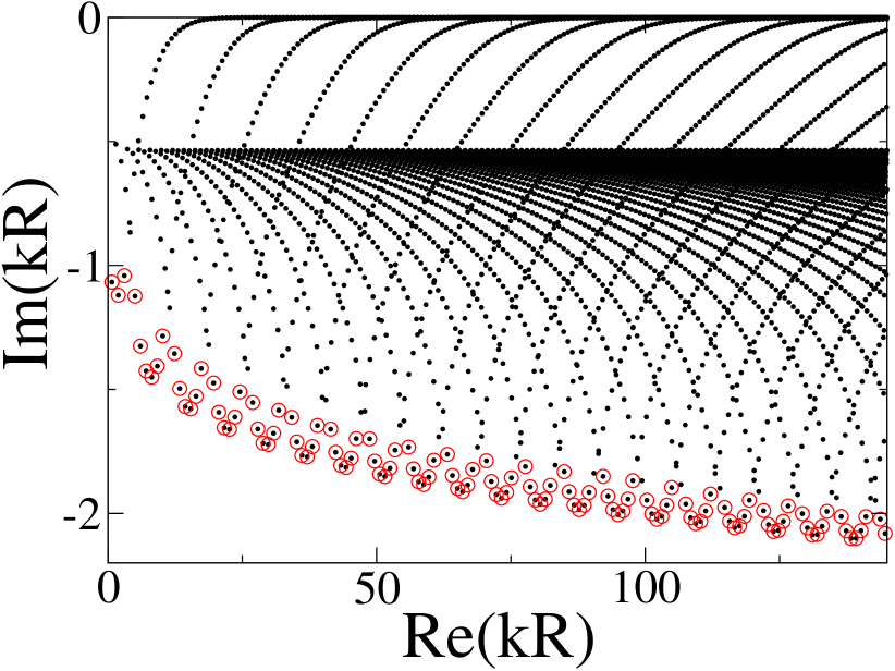
a)

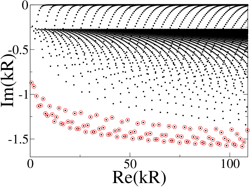
b)

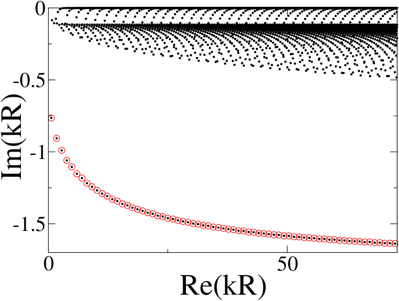
c)

Figure 2: (Color online). Resonance spectra for TE modes of the circular dielectric cavity with $n=1.5$ (a), $n=2$ (b), and $n=3$ (c). The red circles encircle the additional branch of resonances obtained by choosing initial conditions (48) and running a root searching routine to solve the equation $s_{m}(x)=0$ with $s_{m}(x)$ given by (7). The range along the $x$ axis are chosen such that every plot contains around 12000 resonances (counted with multiplicity).

In Fig. 3 we plot the difference between the function counting the numerically computed resonances resonances with a real part less than $k$ (with radius $R=1$) and the best fit to it of the form, see (41),

$$N_{\mathrm{fit}}(k)=\frac{n^{2}}{4}(kR)^{2}+a_{1}(kR)+a_{0}$$ (67)

where $a_{1}$ and $a_{0}$ are fitting parameters.

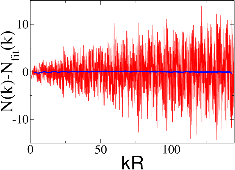
a)

b)

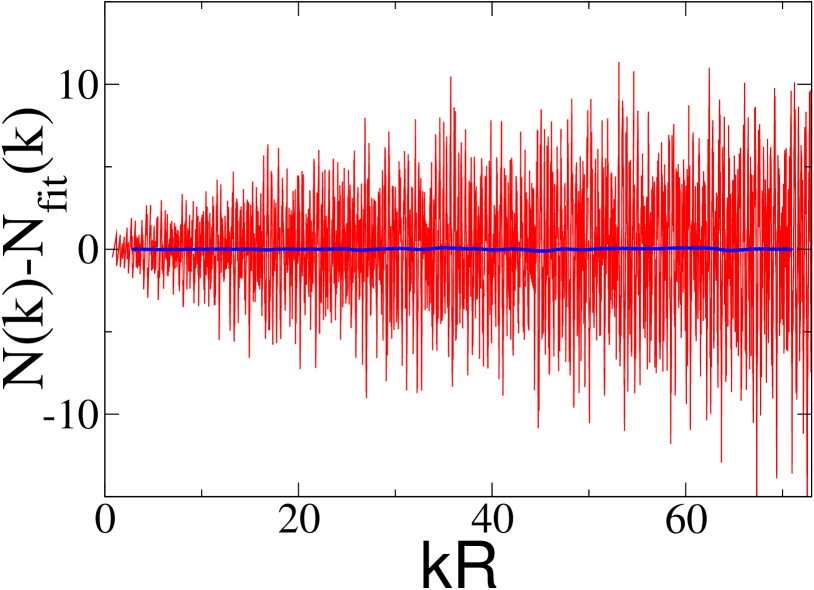
c)

Figure 3: (Color online) Difference between the exact number of resonances and the fit (67) for $n=1.5$ (a), $n=2$ (b), and $n=3$ (c). In the latter case the additional resonances in Fig. 2 c) are not taken into account. The blue solid thick line indicates the difference averaged over a large interval.

For $n=1.5$ and $n=2$ we consider all resonances including the additional branch. For $n=3$ this branch is quite far from the other resonances (cf. Fig. 2 c)) and it is natural not to include it in the counting. The fitted values of the parameters for these three cases are the following

$$\begin{array}[]{lll }n=1.5,&a_{1}=1.246,&a_{0}=-0.66\\ n=2,&a_{1}=1.122,&a_{0}=-0.50\\ n=3,&a_{1}=-1.189,&a_{0}=0.12\end{array}.$$ (68)

The term $a_{1}$ has to be compared with the theoretical prediction which follows from (52) (used with plus sign for $n=1.5$ and $n=2$, and with minus sign for $n=3$)

$$\begin{array}[]{ll}n=1.5,&a_{1}^{\mathrm{th}}=1.247\\ n=2,&a_{1}^{\mathrm{th}}=1.124\\ n=3,&a_{1}^{\mathrm{th}}=-1.190\end{array}.$$ (69)

The agreement with our numerical calculations is very good.

In Fig. 4 the Fourier transform of the resonance density for the circular dielectric cavity with different values of the refractive index is displayed. As expected from the trace formula, this quantity has peaks at the length of classical periodic orbits of the circle. Notice especially that the triangular orbit is not confined for $n=1.5$. Hence the Fresnel reflection coefficient is small and induces damping, which can be clearly seen in Fig. 4 a). As the index grows it is also shown that the contribution of short-period orbits become closer and closer to the one of the closed billiard.

a)

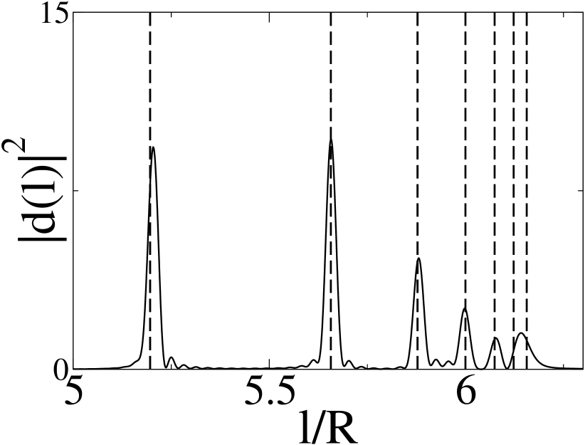
b)

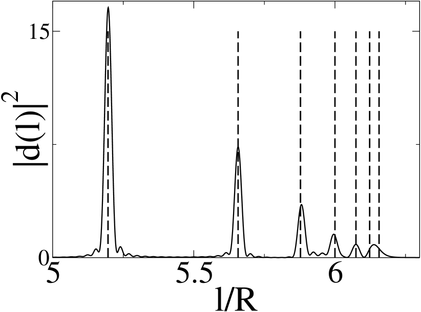
c)

Figure 4: Density of periodic orbit length (Fourier transform of the resonance density) for $n=1.5$ (a), $n=2$ (b), and $n=3$ (c). The vertical lines stand for the length of the shortest periodic orbits of the circular cavity, from left to right: triangle, square, pentagon, hexagon, heptagon and octagon.

In Fig. 5 a) we present the spectrum of the TE resonances for the square cavity of side $a=1$ with $(-\,-)$ symmetry along the diagonals. For such cavity the fit function similar to (67) is

$$N_{\mathrm{fit}}(k)=\frac{n^{2}}{16\pi}(ka)^{2}+a_{1}(ka)+a_{0}$$ (70)

and the best fit gives, see Fig. 5 b),

$$a_{1}=0.0304,\qquad a_{0}=-5.22\ .$$ (71)

The theoretical prediction for this symmetry class is obtained from (53) $a_{1}^{\mathrm{th}}=0.0297$ which agrees well with the numerical calculations.

a)

b)

Figure 5: (Color online) a) Resonance spectrum for the dielectric square with $n=1.5$ for the $(-,-)$ symmetry class. b) The difference between the total number of resonances and the best quadratic fit. The blue solid thick line indicates the difference averaged over a large interval.

Finally the same procedure was done for the dielectric stadium consisted of two half-circles of radius $R$ connected by a rectangle with sides $2\alpha R$ and $2R$ where $\alpha$ called the aspect ratio of the stadium. The calculations were restricted to the symmetry class such that the associated function vanishes along both symmetry axis of the stadium, which is again called $(-,-)$ symmetry class. The resonance spectrum is presented in Fig. 6 a).

a)

b)

Figure 6: (Color online) a) Resonance spectrum for the dielectric stadium with $n=1.5$ for the $(-,-)$ symmetry class. b) The difference between the total number of resonances and the best quadratic fit. The blue solid thick line indicates the difference averaged over a large interval.

The fit function is now

$$N_{\mathrm{fit}}(k)=\frac{n^{2}}{4\pi}\left(\alpha+\frac{\pi}{4}\right)(kR)^{2}+a_{1}(kR)+a_{0}$$ (72)

where the aspect ratio $\alpha$ has been taken to $1$ in the numerical calculations. The best fit gives, see Fig. 6 b),

$$a_{1}=0.150,\quad a_{0}=-5.24\ ,$$ (73)

which agrees well with the prediction for this symmetry class: $a_{1}^{\mathrm{th}}=0.152$ (cf. (53)).

VIII Summary

Trace formulas are the main tool of the semiclassical description of multi-dimensional quantum problems. For closed systems the trace formulas relate two objects: quantum density of discrete states and a sum over classical periodic orbits

$$d(E)\equiv\sum_{n}\delta(E-E_{n})$$

$$\approx\bar{d}(E)+\sum_{\mathrm{period.\ orbits}}A_{p}\mathrm{e}^{\mathrm{i}S_{p}(E)/\hbar}+\mathrm{c.c.}$$ (74)

where $S_{p}(E)$ is the classical action over a periodic orbit and $\bar{d}(E)$ is the mean density of eigen-energies, averaged over a small window around $E$. For 2d billiards with area $\mathcal{A}$ and perimeter $\mathcal{L}$ this averaged density of states is

$$\bar{d}(E)=\frac{\mathcal{A}}{4\pi}+r\frac{\mathcal{L}}{8\pi\sqrt{E}}+o(E^{-1/2})$$ (75)

where $r=1$ for the Neumann boundary conditions and $r=-1$ for the Dirichlet ones.

For open quantum models the true eigen-energy spectrum is continuous and the main object of interest is the discrete spectrum of resonances defined as the poles of the $S$-matrix in the complex plane: $E_{n}=e_{n}-\mathrm{i}\Gamma_{n}/2$ with $e_{n}$ and $\Gamma_{n}$ real. The real part of the resonance energy, $e_{n}$, gives the position of the resonance while its imaginary part, $\Gamma_{n}$, determines the resonance width.

The analogue of the trace formula for open systems has the form similar to (74)

$$\frac{1}{\pi}\sum_{n}\dfrac{\Gamma_{n}/2}{(E-e_{n})^{2}+\Gamma_{n}^{2}/4}$$

$$\approx\bar{d}(E)+\sum_{\mathrm{period.\ orbits}}A_{p}\mathrm{e}^{\mathrm{i}S_{p}(E)/\hbar}+\mathrm{c.c.}\ .$$ (76)

In Ref. trace1 such type of formula has been obtained for a 2d dielectric cavity with transverse magnetic polarization of the field. Here we derive the trace formula for a 2d dielectric cavity but with boundary conditions corresponding to the transverse electric polarization of the electromagnetic field. As expected, the oscillating part of this trace formula is given by the usual periodic orbits weighted in the leading semiclassical order by the Fresnel coefficient corresponding to TE reflection on the cavity boundary (65), (66).

Our main result is the expression for the average resonance density of a dielectric cavity with area $\mathcal{A}$, perimeter $\mathcal{L}$, and refraction index $n$

$$\bar{d}(E)=\frac{\mathcal{A}n^{2}}{4\pi}+r_{\mathrm{TE}}(n)\frac{\mathcal{L}}{8\pi\sqrt{E}}+o(E^{-1/2})$$ (77)

where

$$r_{TE}(n) = 1+\frac{1}{\pi}\int_{-\infty}^{\infty}\tilde{R}_{\mathrm{TE}}(t)\left(\frac{n^{2}}{n^{2}+t^{2}}-\frac{1}{1+t^{2}}\right)\mathrm{d}t$$ (78)

$$\pm \frac{2n}{\sqrt{n^{2}+1}}$$

and $\tilde{R}_{\mathrm{TE}}(t)$ is the Fresnel reflection coefficient for the TE polarization at imaginary momentum

$$\tilde{R}_{\mathrm{TE}}(t)=\frac{\sqrt{n^{2}+t^{2}}-n^{2}\sqrt{1+t^{2}}}{\sqrt{n^{2}+t^{2}}+n^{2}\sqrt{1+t^{2}}}\ .$$ (79)

The plus-minus sign in front of the last term in (78) is connected with the existence for the TE modes of an additional series of resonances related to Brewster’s angle. As these resonances have large imaginary parts, they may be included or not in the counting function. For small values of $n$ additional resonances are mixed with other resonances and their separation is artificial. In this case the plus sign has to be used. For large $n$ the branch of additional resonances is well separated from the body of resonances and it is natural to ignore them. It corresponds to the minus sign in (78).

The results of this paper together with Ref. trace1 demonstrate that semiclassical trace formulas can be derived and applied for open dielectric cavities in a close similarity with closed billiards. Further investigations of trace formulas for other physical open systems is of considerable interest.

Appendix A Krein formula approach

The purpose of this Appendix is to present another derivation of the number of resonances in a circular dielectric cavity based on the Krein spectral shift formula krein_1 . The true eigen-energy spectrum for an open system is continuous and, consequently, the density of states for open quantum systems is infinite. Nevertheless, the difference between the density of states with a cavity and the density of state without the cavity is finite and is given by the Krein formula

$$d(E)-d_{0}(E)=\frac{1}{2\pi\mathrm{i}}\frac{\partial}{\partial E}\ln\det\mathbf{S}(E)$$ (80)

where $\mathbf{S}(E)$ is the $S$-matrix for the scattering on the cavity.

This formula is general and can be used for any type of short-range potential. We apply it for a scattering on a circular dielectric cavity. It is easy to check that the $S$-matrix for the the scattering on 2d circular cavity with TE boundary conditions (5) is diagonal in the polar coordinates and

$$S_{m}(x)=-\frac{\tilde{s}_{m}(x)}{s_{m}(x)}$$ (81)

where $s_{m}(x)$ is given by (7) and $\tilde{s}_{m}(x)$ differs from $s_{m}(x)$ by changing $H_{m}^{(1)}(x)$ to $H_{m}^{(2)}(x)$:

$$\tilde{s}_{m}(x)=x\Big{[}\frac{1}{n}J_{m}^{\prime}(nx)H_{m}^{(2)}(x)-J_{m}(nx)H_{m}^{(2)\,\prime}(x)\Big{]}\ .$$ (82)

From properties of the Bessel functions bateman it is straightforward to show that

$$\frac{s_{m}^{\prime}}{s_{m}}(x)=$$

$$- \dfrac{(n^{2}-1)}{n^{2}}\dfrac{J_{m}(nx)H_{m}^{(1)}(x)m^{2}/x^{2}+nJ_{m}^{\prime}(nx)H_{m}^{(1)\prime}(x)}{J_{m}^{\prime}(nx)H_{m}^{(1)}(x)/n-J_{m}(nx)H_{m}^{(1)\prime}(x)}\ .$$

Using the equality $J_{m}(x)=(H_{m}^{(1)}(x)+H_{m}^{(2)})/2$, this expression can be rewritten in the form

$$\frac{s_{m}^{\prime}}{s_{m}}(x)=-\frac{n^{2}-1}{n^{2}}\dfrac{A_{m}(x)+B_{m}(x)E_{m}(x)}{C_{m}(x)[1-R_{m}(x)E_{m}(x)]}$$ (84)

where $E_{m}(x)$ and $R_{m}(x)$ are defined in (9) and (10) respectively, and

$$A_{m}(x) = \frac{m^{2}}{x^{2}}+n\frac{H_{m}^{(2)\prime}}{H_{m}^{(2)}}(nx)\frac{H_{m}^{(1)\prime}}{H_{m}^{(1)}}(x)\ ,$$ (85)

$$B_{m}(x) = \frac{m^{2}}{x^{2}}+n\frac{H_{m}^{(1)\prime}}{H_{m}^{(1)}}(nx)\frac{H_{m}^{(1)\prime}}{H_{m}^{(1)}}(x)\ ,$$ (86)

$$C_{m}(x) = \frac{H_{m}^{(2)\prime}}{nH_{m}^{(2)}}(nx)-\frac{H_{m}^{(1)\prime}}{H_{m}^{(1)}}(x)\ .$$ (87)

Expanding this expression into series of $E_{m}(x)$ gives

$$\frac{s_{m}^{\prime}}{s_{m}}(x)=Q_{m}(x)+P_{m}\sum_{r=1}^{\infty}R_{m}^{r}(x)\,E_{m}^{r}(x)$$ (88)

where

$$Q_{m}(x)=-\frac{(n^{2}-1)A_{m}(x)}{n^{2}C_{m}(x)}$$ (89)

and

$$P_{m}(x)=-\frac{4\mathrm{i}(n^{2}-1)\Big{[}\frac{m^{2}}{n^{2}x^{2}}+\left(\frac{H_{m}^{(1)\prime}}{H_{m}^{(1)}}(x)\right)^{2}\Big{]}}{\pi n^{2}xH_{m}^{(1)}(nx)H_{m}^{(2)}(nx)C_{m}(x)D_{m}(x)}\ .$$ (90)

with

$$D_{m}(x)=\frac{H_{m}^{(1)\prime}}{nH_{m}^{(1)}}(nx)-\frac{H_{m}^{(1)\prime}}{H_{m}^{(1)}}(x)$$ (91)

In the semiclassical limit $x\to\infty$ the above formulae are simplified by using the asymptotic of the Hankel function (11)

$$\frac{H_{m}^{(1,2)\prime}}{H_{m}^{(1,2)}}(x)\underset{x\to\infty}{\longrightarrow}\pm\mathrm{i}\sqrt{1-\frac{m^{2}}{x^{2}}}-\frac{x}{2(x^{2}-m^{2})}+\mathcal{O}(x^{-2})\ .$$ (92)

Consider first the smooth term (89). From the identity

$$\Big{(}\frac{1}{n^{2}}\sqrt{n^{2}-t^{2}}+\sqrt{1-t^{2}}\Big{)}\Big{(}\sqrt{n^{2}-t^{2}}-\sqrt{1-t^{2}}\Big{)}$$ (93)

$$= \frac{n^{2}-1}{n^{2}}\Big{(}t^{2}+\sqrt{n^{2}-t^{2}}\sqrt{1-t^{2}}\Big{)}$$

it is straightforward to check that

$$Q_{m}(x)\underset{x\to\infty}{\longrightarrow}-\mathrm{i}\left[\sqrt{n^{2}-\frac{m^{2}}{x^{2}}}-\sqrt{1-\frac{m^{2}}{x^{2}}}\right]$$

$$- \frac{x}{2}R_{\mathrm{TE}}\Big{(}\frac{m}{x}\Big{)}\left[\frac{n^{2}}{n^{2}x^{2}-m^{2}}-\frac{1}{x^{2}-m^{2}}\right]$$

where $R_{\mathrm{TE}}(t)$ is the Fresnel reflection coefficient for the TE polarization given by (15).

The difference between the density of state with a cavity and the one without the cavity averaged over an energy interval such that periodic orbit terms are small can be calculated from $Q_{m}(x)$

$$\langle d(E)\rangle-d_{0}(E)=-\frac{R}{2\pi k}\sum_{m=-\infty}^{\infty}\mathrm{Im}\,Q_{m}(x)\ .$$ (95)

Changing the summation over $m$ to the integration and turning the integration contour in the second term in (A) in the complex plane to avoid poles, $m\to-\mathrm{i}t$ leads to

$$\langle d(E)\rangle-d_{0}(E)=$$

$$\frac{R}{2\pi k}\Big{[}\int_{-nx}^{nx}\sqrt{n^{2}-\frac{m^{2}}{x^{2}}}\mathrm{d}m-\int_{-x}^{x}\sqrt{1-\frac{m^{2}}{x^{2}}}\mathrm{d}m\Big{]}$$

$$+ \frac{Rx}{4\pi k}\int_{-\infty}^{\infty}\mathrm{d}tR_{\mathrm{TE}}\Big{(}-\mathrm{i}\frac{t}{x}\Big{)}\Big{[}\frac{n^{2}}{n^{2}x^{2}+t^{2}}-\frac{1}{x^{2}+t^{2}}\Big{]}\ .$$

Rescaling integration variables one gets

$$\langle d(E)\rangle - d_{0}(E)=\frac{\mathcal{A}}{4\pi}(n^{2}-1)$$

$$+ \frac{\mathcal{L}}{8\pi^{2}k}\int_{-\infty}^{\infty}\mathrm{d}t\,\tilde{R}_{\mathrm{TE}}(t)\Big{[}\frac{n^{2}}{n^{2}+t^{2}}-\frac{1}{1+t^{2}}\Big{]}$$

where $\mathcal{A}=\pi R^{2}$ and $\mathcal{L}=2\pi R$ are the area and the perimeter of a circular cavity.

This formula differs form the averaged total number of resonances (41) and (45). This is the consequence of the fact discussed in trace1 for the case of TM modes that the $S$-matrix for the scattering on a cavity has an additional phase (and additional zeros) connected with the outside scattering on the impenetrable cavity.

The form of this ’additional’ $S$-matrix may be argued as follows. It is known that when a wave from outside the cavity scatters on a cavity it reflects with the reflection coefficient which differs by the sign from the reflection coefficient from inside the cavity (this is a consequence of current conservation). For the TE polarization the Fresnel reflection coefficient for a scattering from a medium with the refraction index $1$ on another medium with the refraction index $n$ is $-R_{\mathrm{TE}}$ where $R_{\mathrm{TE}}$ is given by (15). In semiclassical region accessible in outside scattering, $|t|<1$, the reflection coefficient $-R_{\mathrm{TE}}(t)$ is real and the ’effective’ reflection coefficient corresponding to the scattering on impenetrable cavity equals to the sign of $-R_{\mathrm{TE}}(t)$ (cf. (39))

$$R_{\mathrm{TE}}^{(eff)}=\left\{\begin{array}[]{rr}-1,&t^{*}\leq|t|\leq 1\\ 1,&0\leq|t|\leq t^{*}\end{array}\right.$$ (98)

where $t^{*}=n/\sqrt{n^{2}+1}$.

The reflection coefficient equals to $-1$ (resp. $+1$) corresponding to the scattering with Dirichlet (resp. Neumann) conditions on the cavity boundary. For a circular cavity the $S$-matrices with Dirichlet and Neumann boundary conditions are well known (see e.g. uzy )

$$S_{m}^{(D)}(x)=-\frac{H_{m}^{(2)}}{H_{m}^{(1)}}(x),\qquad S_{m}^{(N)}(x)=-\frac{H_{m}^{(2)\prime}}{H_{m}^{(1)\prime}}(x)\ .$$ (99)

The ’additional’ $S$-matrix for the TE scattering is thus formally

$$\det(S^{(\mathrm{TE})}_{0}(x)) = \prod_{m=-\infty}^{-(m^{*}+1)}S_{m}^{(D)}(x)\prod_{m=-m^{*}}^{m^{*}}S_{m}^{(N)}(x)$$ (100)

$$\times \prod_{m=m^{*}+1}^{\infty}S_{m}^{(D)}(x)$$

where $m^{*}=[xn/\sqrt{n^{2}+1}]$.

To find the total phase of this ’additional’ $S$-matrix one can proceed as follows. To the leading order in the semiclassical limit $x\to\infty$ the Dirichlet and Neumann $S$-matrices (99) can be calculated from (11). It gives

$$S_{m}^{(D)}(x)\approx-\mathrm{e}^{-2\mathrm{i}\Phi_{m}(x)}\qquad S_{m}^{(N)}(x)\approx\mathrm{e}^{-2\mathrm{i}\Phi_{m}(x)}$$ (101)

where $\Phi_{m}(x)$ is given by (12). It means that $S_{m}^{(N)}$ differs from $S_{m}^{(D)}$ only by its sign, which is another manifestation of the opposite sign of the reflection coefficient (98). Therefore one can rewrite expression (100) as follows

$$S^{(\mathrm{TE})}_{0}\approx S^{(D)}\prod_{m=-m^{*}}^{m^{*}}(-1)\approx S^{(D)}\mathrm{e}^{\pm 2\mathrm{i}\pi xn/\sqrt{n^{2}+1}}$$ (102)

where $S^{(D)}=\prod_{m=-\infty}^{\infty}S_{m}^{(D)}$ is the full $S$-matrix for the scattering on a cavity with the Dirichlet boundary condition. The $\pm$ sign in the exponent reflects the ambiguity of the phase, $-1=\mathrm{e}^{\pm\mathrm{i}\pi}$.

The calculation of the mean density of states related with $S^{(D)}$-matrix is straightforward (see e.g. uzy )

$$d_{D}(E)-d_{0}(E)=-\frac{\mathcal{A}}{4\pi}-\frac{\mathcal{L}}{8\pi k}$$ (103)

and finally from (102) and the Krein formula (80) one finds that the change of the density of states due to the ’additional’ $S$-matrix (100) is

$$\bar{d}_{0}(E) - d_{0}(E)=d_{D}(E)-d_{0}(E)\pm\frac{\mathcal{L}}{8\pi k}\frac{2n}{\sqrt{n^{2}+1}}$$ (104)

$$= -\frac{\mathcal{A}}{4\pi}-\frac{\mathcal{L}}{8\pi k}\Big{(}1\mp\frac{2n}{\sqrt{n^{2}+1}}\Big{)}\ .$$

The total density of resonances is thus the difference between (A) and (104). In the end one gets Eqs. (41) and (45). The ambiguity in the phase of the ’additional’ $S$-matrix corresponds to the the possibility to include resonances related with Brewster’s angle in the Weyl formula or not which has been discussed in Section V.

References

(1) K. Vahala, ed., Optical microcavities (World
Scientific Press, 2004).
(2) A. B. Matsko, Practical applications of microresonators
in optics and photonics, (CRC Press, Taylor and Francis Group, 2009).
(3) R. Balian, C. Bloch, Ann. Phys. 60, 401
(1970); Ann. Phys. 64, 271 (1971); Ann. Phys. 69, 76
(1972).
(4) M. Gutzwiller, Chaos in classical and quantum
mechanics, (Springer-Verlag, Berlin, Heidelberg, New-York, 1990).
(5) F. Haake, Quantum signatures of chaos,
(Springer-Verlag, Berlin, Heidelberg, New-York, 2001).
(6) P. Lax and R. S. Phillips, Scattering theory,
(Springer, New York, 1963).
(7) R. G. Newton, Scattering theory of waves and
particles, (Springer-Verlag, New York, Heidelberg, Berlin, 1982).
(8) E. Bogomolny, R. Dubertrand, and C. Schmit, Phys. Rev. E
78, 056202 (2008).
(9) E. Bogomolny, N. Djellali, R. Dubertrand, I. Gozhyk, M.
Lebental, C. Schmit, C. Ulysse, and J. Zyss, Phys. Rev. E
83, 036208 (2011).
(10) S. Bittner, E. Bogomolny, B. Dietz, M. Miski-Oglu,
P. Oria Iriarte, A. Richter, F. Schäfer, Phys. Rev. E 81, 066215
(2010); S. Bittner, E. Bogomolny, B. Dietz, M. Miski-Oglu,
A. Richter, Phys. Rev. E 85, 026203 (2012).
(11) J. D. Jackson, Classical electrodynamics, (Wiley,
1999).
(12) M. Lebental, N. Djellali, C. Arnaud,
J.-S. Lauret, J. Zyss, R. Dubertrand, C. Schmit, E. Bogomolny, Phys. Rev. A
76, 023830 (2007).
(13) R. Dubertrand, E. Bogomolny, N. Djellali, M. Lebental,
and C. Schmit, Phys. Rev. A 77, 013804 (2008).
(1997); C. Gmachl, F. Capasso, E. E. Narimanov, J. U. Nöckel,
A. D. Stone, J. Faist, D. L. Sivco and A. Y. Cho, Science 280,
1556 (1998);
V. A. Podolsky, E. Narimanov, W. Fang, and H. Cao, Proc.
Nat. Acad. Sci. USA. 101, 10498 (2004).
(14) H.P. Baltes and E.R. Hilf, Spectra of Finite
Systems, (Bibliographisches
Institut, Mannheim, Wien, Zurich, 1976).
(15) A. Erdelyi, Higher transcendental functions,
Vol. II, (McGraw-Hill Book Company, New York, Toronto, London, 1955).
(16) C. P. Dettmann, G. V. Morozov, M. Sieber, and
H. Waalkens, Europhys. Lett. 87, 34003 (2009).
(17) M.G. Krein, Matem. Sbornik 33, 597 (1953);
Dokl. Akad. Nauk, SSR 144, 268 (1962); English trans. in Soviet
Math. Dokl. 3 (1962).
(18) U. Smilansky and I. Ussishkin, J. Phys. A: Math. Gen.
29, 2587 (1996).