Performance of first-order methods for smooth convex minimization: a novel approach

Abstract

We introduce a novel approach for analyzing the performance of first-order black-box optimization methods. We focus on smooth unconstrained convex minimization over the Euclidean space $\mathbb{R}^{d}$. Our approach relies on the observation that by definition, the worst case behavior of a black-box optimization method is by itself an optimization problem, which we call the Performance Estimation Problem (PEP). We formulate and analyze the PEP for two classes of first-order algorithms. We first apply this approach on the classical gradient method and derive a new and tight analytical bound on its performance. We then consider a broader class of first-order black-box methods, which among others, include the so-called heavy-ball method and the fast gradient schemes. We show that for this broader class, it is possible to derive new numerical bounds on the performance of these methods by solving an adequately relaxed convex semidefinite PEP. Finally, we show an efficient procedure for finding optimal step sizes which results in a first-order black-box method that achieves best performance.

Keywords: Performance of First-Order Algorithms, Rate of Convergence, Complexity, Smooth Convex Minimization, Duality, Semidefinite Relaxations, Fast Gradient Schemes, Heavy Ball method.

1 Introduction

First-order convex optimization methods have recently gained in popularity both in theoretical optimization and in many scientific applications, such as signal and image processing, communications, machine learning, and many more. These problems are very large scale, and first-order methods, which in general involve very cheap and simple computational iterations, are often the best option to tackle such problems in a reasonable time, when moderate accuracy solutions are sufficient. For convex optimization problems, there exists an extensive literature on the development and analysis of first-order methods, and in recent years, this has been revitalized at a quick pace due to the emergence of many fundamental new applications alluded above, see e.g., the recent collections [15, 18] and references therein.

This work is not on the development of new algorithms, rather it focuses on the theoretical performance analysis of first order methods for unconstrained minimization with an objective function which is known to belong to a given family $\mathcal{F}$ of smooth convex functions over the Euclidean space $\mathbb{R}^{d}$, the function itself is not known.

Following the seminal work of Nemirovski and Yudin [12] in the complexity analysis of convex optimization methods, we measure the computational cost based on the oracle model of optimization. According to this model, a first-order black-box optimization method is an algorithm which has knowledge of the underlying space $\mathbb{R}^{d}$ and the family $\mathcal{F}$, the function itself is not known. To gain information on the function to be minimized, the algorithm queries a first order oracle, that is, a subroutine which given as input a point in $\mathbb{R}^{d}$, returns the value of the objective function and its gradient at that point. The algorithm thus generates a finite sequence of points $\{x_{i}\in\mathbb{R}^{d}:i=0,\dots,N\}$, where at each step the algorithm can depend only on the previous steps, their function values and gradients via some rule

$$x_{0}\in\mathbb{R}^{d},\;x_{i+1}={\cal A}(x_{0},\dots,x_{i};f(x_{0}),\dots,f(x_{i});f^{\prime}(x_{0}),\dots,f^{\prime}(x_{i})),\;i=0,\ldots,N-1,$$

where $f^{\prime}(\cdot)$ stands for the gradient of $f(\cdot)$. Note that the algorithm has another implicit knowledge, i.e., that the distance from its initial point $x_{0}$ to a minimizer $x_{\ast}\in X_{\ast}(f)$ of $f$ is bounded by some constant $R>0$, see more precise definitions in the next section.

Given a desired accuracy $\varepsilon>0$, applying the given algorithm on the function $f$ in the class $\mathcal{F}$, the algorithm stops when it produces an approximate solution $x_{\varepsilon}$ which is $\varepsilon$-optimal, that is such that

$$f(x_{\epsilon})-f(x_{\ast})\leq\epsilon.$$

The performance (or complexity) of a first order black-box optimization algorithm is then measured by the number of oracle calls the algorithm needs to find such an approximate solution. Equivalently, we can measure the performance of an algorithm by looking at the absolute inaccuracy

$$\delta(f,x_{N})=f(x_{N})-f(x_{\ast}),$$

where $x_{N}$ is the result of the algorithm after making $N$ calls to the oracle. Throughout this paper we will use the latter form to measure the performance of a given algorithm.

Building on this model, in this work we introduce a novel approach for analyzing the performance of a given first order scheme. Our approach relies on the observation that by definition, the worst case behavior of a first-order black-box optimization algorithm is by itself an optimization problem which consists of finding the maximal absolute inaccuracy over all possible inputs to the algorithm. Thus, with $x_{N}$ being the output of the algorithm after making $N$ calls to the oracle, we look at the solution of the following Performance Estimation Problem (PEP):

$$\begin{aligned} \max\quad&f(x_{N})-f(x_{\ast})\\ \text{s.t. }\quad&f\in\mathcal{F},\\ &x_{i+1}={\cal A}(x_{0},\dots,x_{i};f(x_{0}),\dots,f(x_{i});f^{\prime}(x_{0}),\dots,f^{\prime}(x_{i})),\;i=0,\ldots,N-1,\\ &x_{\ast}\in X_{\ast}(f),\|x_{\ast}-x_{0}\|\leq R\\ &x_{0},\ldots,x_{N},x_{\ast}\in\mathbb{R}^{d}.\end{aligned}$$ (P)

At first glance this problem seems very hard or impossible to solve. We overcome this difficulty through an analysis that relies on various types of relaxations, including duality and semi-definite relaxation techniques. The problem and setting, and an outline of the underlying idea of the proposed approach for analyzing (P) are described in Section 2. In order to develop the basic idea and tools underlying our proposed approach, we first focus on the fundamental gradient method (GM) for smooth convex minimization, and then extend it to a broader class of first order black box minimization methods. Obviously, the gradient method is a particular case of this broader class that will be analyzed below. However, it is quite important to start with the gradient method for two reasons. First, it allows to acquaint the reader in a more transparent way with the techniques and methodolgy we need to develop in order to analyze (PEP), thus paving the way to tackle more general schemes. Secondly, for the gradient method, we are able to prove a new and tight bound on its performance which is given analytically, see Section 3. Capitalizing on the methodology and tools developed in the past section, in Section 4, we consider a broader class of first-order black-box methods, which among others, is shown to include the so-called heavy-ball [16] and fast gradient schemes [14]. Although an analytical solution is not available for this general case, we show that for this broader class of methods, it is always possible to compute numerical bounds for an adequate relaxation of the corresponding PEP, allowing to derive new bounds on the performance of these methods. We then derive in Section 5 an efficient procedure for finding optimal step sizes which results in a first-order method that achieves best performance. Our approach and analysis give rise to some interesting problems leading us to suggest some conjectures. Finally, an appendix includes the proof of a technical result.

Notation.

For a differentiable function $f$, its gradient at $x$ is denoted by $f^{\prime}(x)$. The Euclidean norm of a vector $x\in\mathbb{R}^{d}$ is denoted as $\|x\|$. The set of symmetric matrices in $\mathbb{R}^{n\times n}$ is denoted by $\mathbb{S}^{n}$. For two symmetric matrices $A$ and $B$, $A\succeq B,(A\succ B)$ means $A-B\succeq 0\,(A-B\succ 0)$ is positive semidefinite (positive definite). We use $e_{i}$ for the $i$-th canonical basis vector in $\mathbb{R}^{N}$, which consists of all zero components, except for its $i$-th entry which is equal to one, and use $\nu$ to denote a unit vector in $\mathbb{R}^{d}$. For an optimization problem (P), $\operatorname{val}(P)$ stands for its optimal value.

2 The Problem and the Main Approach

2.1 The Problem and Basic Assumptions

Let $\mathcal{A}$ be a first-order algorithm for solving the optimization problem

$$\begin{aligned} (M)\quad\min\{f(x):\,x\in\mathbb{R}^{d}\}.\end{aligned}$$

Throughout the paper we make the following assumptions:

• $f:\mathbb{R}^{d}\to\mathbb{R}$ is a convex function of the type $C^{1,1}_{L}(\mathbb{R}^{d})$, i.e., continuously differentiable with Lipschitz continuous gradient:

  $$\|f^{\prime}(x)-f^{\prime}(y)\|\leq L\|x-y\|,\,\,\forall x,y\in\mathbb{R}^{d},$$

  where $L>0$ is the Lipschitz constant.

• We assume that (M) is solvable, i.e., the optimal set $X_{*}(f):=\operatorname*{arg\,min}f$ is nonempty, and for $x_{*}\in X_{*}(f)$ we set $f^{*}:=f(x_{*}).$

• There exists $R>0$, such that the distance from $x_{0}$ to an optimal solution $x_{\ast}\in X_{*}(f)$ is bounded by $R$.

Given a convex function $f$ in the class $C^{1,1}_{L}(\mathbb{R}^{d})$ and any starting point $x_{0}\in\mathbb{R}^{d}$, the algorithm $\mathcal{A}$ is a first-order black box scheme, i.e., it is allowed to access $f$ only through the sequential calls to the first order oracle that returns the value and the gradient of $f$ at any input point $x$. The algorithm $\mathcal{A}$ then generates a sequence of points $x_{i}\in\mathbb{R}^{d},\;i=0,\ldots,N$.

2.2 Basic Idea and Main Approach

We are interested in measuring the worst-case behavior of a given algorithm $\mathcal{A}$ in terms of the absolute inaccuracy $f(x_{N})-f(x_{\ast})$, by solving problem (P) defined in the introduction, namely

$$\begin{aligned} \max\quad&f(x_{N})-f(x_{\ast})\\ \text{s.t. }\quad&f\in C^{1,1}_{L}(\mathbb{R}^{d})\text{, $f$ is convex},\\ &x_{i+1}={\cal A}(x_{0},\dots,x_{i};f(x_{0}),\dots,f(x_{i});f^{\prime}(x_{0}),\dots,f^{\prime}(x_{i})),\;i=0,\ldots,N-1,\\ &x_{\ast}\in X_{\ast}(f),\|x_{\ast}-x_{0}\|\leq R,\\ &x_{0},\ldots,x_{N},x_{\ast}\in\mathbb{R}^{d}.\end{aligned}$$ (P)

To tackle this problem, we suggest to perform a series of relaxations thereby reaching a tractable optimization problem.

A main difficulty in problem (P) lies in the functional constraint ($f$ is a convex function in $C^{1,1}_{L}(\mathbb{R}^{d})$), i.e., we are facing an abstract hard optimization problem in infinite dimension. To overcome this difficulty, the approach taken in this paper is to relax this constraint so that the problem can be reduced and formulated as an explicit finite dimensional problem that can eventually be adequately analyzed.

An un-formal description of the underlying idea consists of two main steps as follows:

• Given an algorithm ${\cal A}$ that generates a finite sequence of points, to build a problem in finite dimension we replace the functional constraint $f\in C^{1,1}_{L}$ in (P) by new variables in $\mathbb{R}^{d}$. These variables, are the points $\{x_{0},x_{1},\ldots x_{N},x_{\ast}\}$ themselves, the function values and their gradients at these points. Roughly speaking, this can be seen as a sort of discretization of $f$ at a selected set of points.

• To define constraints that relate the new variables, we use relevant/useful properties characterizing the family of convex functions in $C^{1,1}_{L}$, as well as the rule(s) describing the given algorithm ${\cal A}$.

This approach can, in principle, be applied to any optimization algorithm. Note that any relaxation performed on the maximization problem (P) may increase its optimal value, however, the optimal value of the relaxed problem still remains a valid upper bound on $f(x_{N})-f^{\ast}$.

A formal description on how this approach can be applied to the gradient method is described in the next section, which as we shall see, allows us to derive a new tight bound on the performance of the gradient method.

3 An Analytical Bound for the Gradient Method

To develop the basic idea and tools underlying the proposed approach for analyzing the performance of iterative optimization algorithms, in this section we focus on the simplest fundamental method for smooth convex minimization, the Gradient Method (GM). It will also pave the way to tackle more general first-order schemes as developed in the forthcoming sections.

3.1 A Performance Estimation Problem for the Gradient Method

Consider the gradient algorithm with constant step size, as applied to problem $(M)$, which generates a sequence of points as follows:

Algorithm GM 0. Input: $f\in C^{1,1}_{L}(\mathbb{R}^{d})$ convex, $x_{0}\in\mathbb{R}^{d}.$ 1. For $i=0,\dots,N-1$, compute $x_{i+1}=x_{i}-\frac{h}{L}f^{\prime}(x_{i})$.

Here $h>0$ is fixed. At this point, we recall that for $h=1$, the convergence rate of the GM algorithm can be shown to be (see for example [14, 4]):

$$f(x_{N})-f^{\ast}\leq\frac{L\|x_{0}-x_{\ast}\|^{2}}{2N},\quad\forall x_{\ast}\in X_{\ast}(f).$$ (3.1)

To begin our analysis, we first recall a fundamental well-known property for the class of convex $C^{1,1}_{L}$ functions, see e.g., [14, Theorem 2.1.5].

Proposition 3.1.

Let $f:\mathbb{R}^{d}\to\mathbb{R}$ be convex and $C^{1,1}_{L}$. Then,

$$\frac{1}{2L}\|f^{\prime}(x)-f^{\prime}(y)\|^{2}\leq f(x)-f(y)-\langle f^{\prime}(y),x-y\rangle,\;\mbox{for all}\;x,y\in\mathbb{R}^{d}.$$ (3.2)

Let $x_{0}\in\mathbb{R}^{d}$ be any starting point, let $\{x_{1},\dots,x_{N}\}$ be the points generated by Algorithm (GM) and let $x_{\ast}$ be a minimizer of $f$. Applying (3.2) on the points $\{x_{0},\dots,x_{N},x_{\ast}\}$, we get:

$$\frac{1}{2L}\|f^{\prime}(x_{i})-f^{\prime}(x_{j})\|^{2}\leq f(x_{i})-f(x_{j})-\langle f^{\prime}(x_{j}),x_{i}-x_{j}\rangle,\quad i,j=0,\dots,N,\ast.$$ (3.3)

Now define

$$\delta_{i} :=\frac{1}{L\|x_{\ast}-x_{0}\|^{2}}(f(x_{i})-f(x_{\ast})),\quad i=0,\dots,N,\ast$$

$$g_{i} :=\frac{1}{L\|x_{\ast}-x_{0}\|}f^{\prime}(x_{i}),\quad i=0,\dots,N,\ast$$

and note that we always have $\delta_{\ast}=0$ and $g_{\ast}=0$.

In terms of $\delta_{i}$, $g_{i}$, condition (3.3) becomes

$$\frac{1}{2}\|g_{i}-g_{j}\|^{2}\leq\delta_{i}-\delta_{j}-\frac{\langle g_{j},x_{i}-x_{j}\rangle}{\|x_{\ast}-x_{0}\|},\quad i,j=0,\dots,N,\ast,$$ (3.4)

and the recurrence defining (GM) reads:

$$x_{i+1}=x_{i}-h\|x_{\ast}-x_{0}\|g_{i},\quad i=0,\ldots,N-1.$$

Problem (P) can now be relaxed by discarding the underlying function $f\in C^{1,1}_{L}$ in (P). That is, the constraint in the function space $f\in C^{1,1}_{L}$ with $f$ convex, is replaced by the inequalities (3.4) characterizing this family of functions and expressed in terms of the variables $x_{0},\dots,x_{N},x_{\ast}\in\mathbb{R}^{d}$, $g_{0},\dots,g_{N}\in\mathbb{R}^{d}$ and $\delta_{0},\dots,\delta_{N}\in\mathbb{R}$ generated by (GM). Thus, an upper bound on the worst case behavior of $f(x_{N})-f(x_{\ast})=L\|x_{\ast}-x_{0}\|^{2}\delta_{N}$ can be obtained by solving the following relaxed PEP:

$$\max_{\begin{subarray}{c}x_{0},\dots,x_{N},x_{\ast}\in\mathbb{R}^{d},\\ g_{0},\dots,g_{N}\in\mathbb{R}^{d},\\ \delta_{0},\dots,\delta_{N}\in\mathbb{R}\end{subarray}}\ L\|x_{\ast}-x_{0}\|^{2}\delta_{N}$$

s.t. $$x_{i+1}=x_{i}-h\|x_{\ast}-x_{0}\|g_{i},\quad i=0,\dots,N-1,$$

$$\frac{1}{2}\|g_{i}-g_{j}\|^{2}\leq\delta_{i}-\delta_{j}-\frac{\langle g_{j},x_{i}-x_{j}\rangle}{\|x_{\ast}-x_{0}\|},\quad i,j=0,\dots,N,\ast,$$

$$\|x_{\ast}-x_{0}\|\leq R.$$

Simplifying the PEP

The obtained problem remains nontrivial to tackle. We will now perform some simplifications on this problem that will be useful for the forthcoming analysis.

First, we observe that the problem is invariant under the transformation $g_{i}^{\prime}\leftarrow Qg_{i}$, $x_{i}^{\prime}\leftarrow Qx_{i}$ for any orthogonal transformation $Q$. We can therefore assume without loss of generality that $x_{\ast}-x_{0}=\|x_{\ast}-x_{0}\|\nu$, where $\nu$ is any given unit vector in $\mathbb{R}^{d}$. Therefore, for $i=\ast$ the inequality constraints reads

$$\frac{1}{2}\|g_{\ast}-g_{j}\|^{2}\leq\delta_{\ast}-\delta_{j}-\frac{\langle g_{j},\|x_{\ast}-x_{0}\|\nu+x_{0}-x_{j}\rangle}{\|x_{\ast}-x_{0}\|},\quad j=0,\dots,N.$$

Secondly, we consider (3.4) for the four cases $i=\ast$, $j=\ast$, $i<j$ and $j<i$, and use the equality constraints

$$x_{i+1}=x_{i}-h\|x_{\ast}-x_{0}\|g_{i},\quad i=0,\dots,N-1$$

to eliminate the variables $x_{1},\dots,x_{N}$. After some algebra, we reach the following form for the PEP:

$$\begin{aligned} \max_{x_{0},x_{\ast},g_{i}\in\mathbb{R}^{d},\delta_{i}\in\mathbb{R}}\ &L\|x_{\ast}-x_{0}\|^{2}\delta_{N}\\ \text{s.t. }&\frac{1}{2}\|g_{i}-g_{j}\|^{2}\leq\delta_{i}-\delta_{j}-\langle g_{j},\sum_{t=i+1}^{j}hg_{t-1}\rangle,\quad i<j=0,\dots,N,\\ &\frac{1}{2}\|g_{i}-g_{j}\|^{2}\leq\delta_{i}-\delta_{j}+\langle g_{j},\sum_{t=j+1}^{i}hg_{t-1}\rangle,\quad j<i=0,\dots,N,\\ &\frac{1}{2}\|g_{i}\|^{2}\leq\delta_{i},\quad i=0,\dots,N,\\ &\frac{1}{2}\|g_{i}\|^{2}\leq-\delta_{i}-\langle g_{i},\nu+\sum_{t=1}^{i}hg_{t-1}\rangle,\quad i=0,\dots,N,\\ &\|x_{\ast}-x_{0}\|\leq R,\end{aligned}$$

where $i<j=0,\dots,N$ is a shorthand notation for $i=0,\dots,N-1,j=i+1,\dots,N$.

Finally, we note that the optimal solution for this problem is attained when $\|x_{\ast}-x_{0}\|=R$, and hence we can also eliminate the variables $x_{0}$ and $x_{\ast}$. This produces the following PEP for the gradient method, a nonconvex quadratic minimization problem:

$$\begin{aligned} \max_{g_{i}\in\mathbb{R}^{d},\delta_{i}\in\mathbb{R}}\ &LR^{2}\delta_{N}\\ \text{s.t. }&\frac{1}{2}\|g_{i}-g_{j}\|^{2}\leq\delta_{i}-\delta_{j}-\langle g_{j},\sum_{t=i+1}^{j}hg_{t-1}\rangle,\quad i<j=0,\dots,N,\\ &\frac{1}{2}\|g_{i}-g_{j}\|^{2}\leq\delta_{i}-\delta_{j}+\langle g_{j},\sum_{t=j+1}^{i}hg_{t-1}\rangle,\quad j<i=0,\dots,N,\\ &\frac{1}{2}\|g_{i}\|^{2}\leq\delta_{i},\quad i=0,\dots,N,\\ &\frac{1}{2}\|g_{i}\|^{2}\leq-\delta_{i}-\langle g_{i},\nu+\sum_{t=1}^{i}hg_{t-1}\rangle,\quad i=0,\dots,N.\\ \end{aligned}$$

This problem can be written in a more compact and useful form. Let $G$ denote the $(N+1)\times d$ matrix whose rows are $g_{0}^{T},\dots g_{N}^{T}$, and for notational convenience let $u_{i}\in\mathbb{R}^{N+1}$ denote the canonical unit vector

$$u_{i}=e_{i+1},\quad i=0,\dots,N.$$

Then for any $i,j$, we have

$$g_{i}=G^{T}u_{i},\;\operatorname{tr}(G^{T}u_{i}u_{j}^{T}G)=\langle g_{i},g_{j}\rangle,\;\mbox{and}\;\langle G^{T}u_{i},\nu\rangle=\langle g_{i},\nu\rangle.$$

Therefore, by defining the following $(N+1)\times(N+1)$ symmetric matrices

$$A_{i,j} =\frac{1}{2}(u_{i}-u_{j})(u_{i}-u_{j})^{T}+\frac{1}{2}\sum_{t=i+1}^{j}h(u_{j}u_{t-1}^{T}+u_{t-1}u_{j}^{T}),$$ (3.5)

$$B_{i,j} =\frac{1}{2}(u_{i}-u_{j})(u_{i}-u_{j})^{T}-\frac{1}{2}\sum_{t=j+1}^{i}h(u_{j}u_{t-1}^{T}+u_{t-1}u_{j}^{T}),$$

$$C_{i} =\frac{1}{2}u_{i}u_{i}^{T},$$

$$D_{i} =\frac{1}{2}u_{i}u_{i}^{T}+\frac{1}{2}\sum_{t=1}^{i}h(u_{i}u_{t-1}^{T}+u_{t-1}u_{i}^{T}),$$

we can express our nonconvex quadratic minimization problem in terms of $\delta:=(\delta_{0},\dots,\delta_{N})\in\mathbb{R}^{N+1}$ and the new matrix variable $G\in\mathbb{R}^{(N+1)\times d}$ as follows

$$\begin{aligned} \max_{G\in\mathbb{R}^{(N+1)\times d},\delta\in\mathbb{R}^{N+1}}\ &LR^{2}\delta_{N}\\ \text{s.t. }&\operatorname{tr}(G^{T}A_{i,j}G)\leq\delta_{i}-\delta_{j},\quad i<j=0,\dots,N,\\ &\operatorname{tr}(G^{T}B_{i,j}G)\leq\delta_{i}-\delta_{j},\quad j<i=0,\dots,N,\\ &\operatorname{tr}(G^{T}C_{i}G)\leq\delta_{i},\quad i=0,\dots,N,\\ &\operatorname{tr}(G^{T}D_{i}G+\nu u_{i}^{T}G)\leq-\delta_{i},\quad i=0,\dots,N.\end{aligned}$$ (G)

Problem (G) is a nonhomogeneous Quadratic Matrix Program, a class of problems recently introduced and studied by Beck [3].

3.2 A Tight Performance Estimate for the Gradient Method

We now proceed to establish the two main results of this section. First, we derive an upper bound on the performance of the gradient method, this is accomplished via using duality arguments. Then, we show that this bound can actually be attained by applying the gradient method on a specific convex function in the class $C^{1,1}_{L}$.

In order to simplify the following analysis, we will remove some constraints from (G) and consider the bound produced by the following relaxed problem:

$$\begin{aligned} \max_{G\in\mathbb{R}^{(N+1)\times d},\delta\in\mathbb{R}^{N+1}}\ &LR^{2}\delta_{N}\\ \text{s.t. }&\operatorname{tr}(G^{T}A_{i-1,i}G)\leq\delta_{i-1}-\delta_{i},\quad i=1,\dots,N,\\ &\operatorname{tr}(G^{T}D_{i}G+\nu u_{i}^{T}G)\leq-\delta_{i},\quad i=0,\dots,N.\end{aligned}$$ (G^′)

As we shall show below, it turns out that this additional relaxation has no damaging effects and produces the desired performance bound when $0<h\leq 1$.

We are interested in deriving a dual problem for (G^′) which is as simple as possible, especially with respect to its dimension. As noted earlier, problem (G^′) is a nonhomogeneous quadratic matrix program, and a dual problem for (G^′) could be directly obtained by applying the results developed by Beck [3]. However, the resulting obtained dual will involve an additional matrix variable $\Phi\in\mathbb{S}^{d}$, where $d$ can be very large. Instead, here by exploiting the special structure of the second set of nonhomogeneous inequalities given in (G^′), we derive an alternative dual problem, but with only one additional variable $t\in\mathbb{R}$.

To establish our dual result, the next lemma shows that a dimension reduction is possible when minimizing a quadratic matrix function sharing the special form as the one that appears in problem (G^′).

Lemma 3.1.

Let $f(X)=\operatorname{tr}(X^{T}QX+2ba^{T}X)$ be a quadratic function, where $X\in\mathbb{R}^{n\times m}$, $Q\in\mathbb{S}^{n}$, $a\in\mathbb{R}^{n}$ and $0\neq b\in\mathbb{R}^{m}$. Then

$$\inf_{X\in\mathbb{R}^{n\times m}}f(X)=\inf_{\xi\in\mathbb{R}^{n}}f(\xi b^{T}).$$

Proof.

First, we recall (this can be easily verified) that $\inf\{f(X):X\in\mathbb{R}^{n\times m}\}>-\infty$ if and only if $Q\succeq 0$, and there exists at least one solution ${\bar{X}}$ such that

$$Q{\bar{X}}+ab^{T}=0\;\Leftrightarrow\;{\bar{X}}^{T}Q+ba^{T}=0,$$ (3.6)

i.e., the above is just $\nabla f(X)=0$ and characterizes the minimizers of the convex function $f(X)$. Using (3.6) it follows that $\inf_{X}f(X)=f({\bar{X}})=\operatorname{tr}(ba^{T}{\bar{X}})$. Now, for any $\xi\in\mathbb{R}^{n}$, we have $f(\xi b^{T})=\|b\|^{2}(\xi^{T}Q\xi+2a^{T}\xi)$. Thus, likewise, $\inf\{f(\xi b^{T}):\xi\in\mathbb{R}^{n}\}>-\infty$ if and only if $Q\succeq 0$ and there exists ${\bar{\xi}}\in\mathbb{R}^{n}$ such that

$$Q{\bar{\xi}}+a=0,$$ (3.7)

and using (3.7) it follows $\inf_{\xi}f(\xi b^{T})=f({\bar{\xi}}b^{T})=\|b\|^{2}a^{T}{\bar{\xi}}=\operatorname{tr}(ba^{T}{\bar{\xi}}b^{T})$. Now, using (3.6)-(3.7), one obtains ${\bar{X}}^{T}Q=-ba^{T}$ and $Q({\bar{X}}-{\bar{\xi}}b^{T})=0$, and hence it follows that

$$f({\bar{X}})-f({\bar{\xi}}) = \operatorname{tr}(ba^{T}({\bar{X}}-{\bar{\xi}}b^{T}))$$

$$= \operatorname{tr}(-{\bar{X}}^{T}Q({\bar{X}}-{\bar{\xi}}b^{T})=0.$$

∎

Equipped with Lemma 3.1, we now derive a Lagrangian dual for problem (G^′).

Lemma 3.2.

Consider problem (G^′) for any fixed $h\in\mathbb{R}$ and $L,R>0$. A Lagrangian dual of (G^′) is given by the following convex program:

$$\begin{aligned} \min_{\lambda\in\mathbb{R}^{N},t\in\mathbb{R}}\{\frac{1}{2}LR^{2}t:\;\lambda\in\Lambda,\;S(\lambda,t)\succeq 0\},\end{aligned}$$ (DG^′)

where $\Lambda:=\{\lambda\in\mathbb{R}^{N}:\;\lambda_{i+1}-\lambda_{i}\geq 0,\quad i=1,\dots,N-1,\;1-\lambda_{N}\geq 0,\;\lambda_{i}\geq 0,\quad i=1,\dots,N\}$, the matrix $S(\cdot,\cdot)\in\mathbb{S}^{N+2}$ is given by

$$S(\lambda,t)=\begin{pmatrix}(1-h)S_{0}+hS_{1}&q\\ q^{T}&t\end{pmatrix},$$

with $q=(\lambda_{1},\lambda_{2}-\lambda_{1},\dots,\lambda_{N}-\lambda_{N-1},1-\lambda_{N})^{T}$ and where the matrices $S_{0},S_{1}\in\mathbb{S}^{N+1}$ are defined by:

$$S_{0}=\begin{pmatrix}2\lambda_{1}&-\lambda_{1}\\ -\lambda_{1}&2\lambda_{2}&-\lambda_{2}\\ &-\lambda_{2}&2\lambda_{3}&-\lambda_{3}\\ &&\ddots&\ddots&\ddots\\ &&&-\lambda_{N-1}&2\lambda_{N}&-\lambda_{N}\\ &&&&-\lambda_{N}&1\\ \end{pmatrix}$$ (3.8)

and

$$S_{1}=\begin{pmatrix}2\lambda_{1}&\lambda_{2}-\lambda_{1}&\dots&\lambda_{N}-\lambda_{N-1}&1-\lambda_{N}\\ \lambda_{2}-\lambda_{1}&2\lambda_{2}&&\lambda_{N}-\lambda_{N-1}&1-\lambda_{N}\\ \vdots&&\ddots&&\vdots\\ \lambda_{N}-\lambda_{N-1}&\lambda_{N}-\lambda_{N-1}&&2\lambda_{N}&1-\lambda_{N}\\ 1-\lambda_{N}&1-\lambda_{N}&\dots&1-\lambda_{N}&1\\ \end{pmatrix}.$$ (3.9)

Proof.

For convenience, we recast (G^′) as a minimization problem, and we also omit the fixed term $LR^{2}$ from the objective. That is, we consider the equivalent problem (G^′′) defined by

$$\begin{aligned} \min_{G\in\mathbb{R}^{(N+1)\times d},\delta\in\mathbb{R}^{N+1}}\ &-\delta_{N}\\ \text{s.t. }&\operatorname{tr}(G^{T}A_{i-1,i}G)\leq\delta_{i-1}-\delta_{i},\quad i=1,\dots,N,\\ &\operatorname{tr}(G^{T}D_{i}G+\nu u_{i}^{T}G)\leq-\delta_{i},\quad i=0,\dots,N.\end{aligned}$$ (G^′′)

Attaching the dual multipliers $\lambda=(\lambda_{1},\dots,\lambda_{N})\in\mathbb{R}^{N}_{+}$ and $\tau:=(\tau_{0},\ldots,\tau_{N})^{T}\in\mathbb{R}^{N+1}_{+}$ to the first and second set of inequalities respectively, and using the notation $\delta=(\delta_{0},\ldots,\delta_{N})$, we get that the Lagrangian of this problem is given as a sum of two separable functions in the variables $(\delta,G)$:

$$L(G,\delta,\lambda,\tau) = -\delta_{N}+\sum_{i=1}^{N}\lambda_{i}(\delta_{i}-\delta_{i-1})+\sum_{i=0}^{N}\tau_{i}\delta_{i}$$

$$+\sum_{i=1}^{N}\lambda_{i}\operatorname{tr}(G^{T}A_{i-1,i}G)+\sum_{i=0}^{N}\tau_{i}\left(\operatorname{tr}(G^{T}D_{i}G+\nu u_{i}^{T}G)\right)$$

$$\equiv L_{1}(\delta,\lambda,\tau)+L_{2}(G,\lambda,\tau).$$

The dual objective function is then defined by

$$H(\lambda,\tau)=\min_{G,\delta}L(G,\delta,\lambda\,\tau)=\min_{\delta}L_{1}(\delta,\lambda,\tau)+\min_{G}L_{2}(G,\lambda,\tau),$$

and the dual problem of (G^′′) is then given by

$$\begin{aligned} \max\{H(\lambda,\tau):\;\lambda\in\mathbb{R}^{N}_{+},\tau\in\mathbb{R}^{N+1}_{+}\}.\end{aligned}$$ (DG^′′)

Since $L_{1}(\cdot,\lambda,\tau)$ is linear in $\delta$, we have $\min_{\delta}L_{1}(\delta,\lambda,\tau)=0$ whenever

$$-\lambda_{1}+\tau_{0} = 0,$$

$$\lambda_{i}-\lambda_{i+1}+\tau_{i} = 0\quad(i=1,\dots,N-1),$$ (3.10)

$$-1+\lambda_{N}+\tau_{N} = 0,$$

and $-\infty$ otherwise. Invoking Lemma 3.1, we get

$$\min_{G\in\mathbb{R}^{(N+1)\times d}}L_{2}(G,\lambda,\tau)=\min_{w\in\mathbb{R}^{N+1}}L_{2}(w\nu^{T},\lambda,\tau).$$

Therefore for any $(\lambda,\tau)$ satisfying (3.10), we have obtained that the dual objective reduces to

$$H(\lambda,\tau) = \min_{w\in\mathbb{R}^{N+1}}\{w^{T}\left(\sum_{i=1}^{N}\lambda_{i}A_{i-1,i}+\sum_{i=0}^{N}\tau_{i}D_{i}\right)w+\tau^{T}w\}$$

$$= \max_{t\in\mathbb{R}}\{-\frac{1}{2}t:w^{T}\left(\sum_{i=1}^{N}\lambda_{i}A_{i-1,i}+\sum_{i=0}^{N}\tau_{i}D_{i}\right)w+\tau^{T}w\leq-\frac{1}{2}t,\ \forall w\in\mathbb{R}^{N+1}\}$$

$$= \max_{t\in\mathbb{R}}\left\{-\frac{1}{2}t:\begin{pmatrix}\sum_{i=1}^{N}\lambda_{i}A_{i-1,i}+\sum_{i=0}^{N}\tau_{i}D_{i}&\frac{1}{2}\tau\\ \frac{1}{2}\tau^{T}&\frac{1}{2}t\end{pmatrix}\succeq 0\right\}.$$

where the last equality follows from the well known lemma [6, Page 163].

Now, recalling the definition of the matrices $A_{i-1,i},D_{i}$ (see (3.5)), we obtain

$$\sum_{i=1}^{N}\lambda_{i}A_{i-1,i}=\frac{1}{2}\begin{pmatrix}\lambda_{1}&(h-1)\lambda_{1}\\ (h-1)\lambda_{1}&\lambda_{1}+\lambda_{2}&(h-1)\lambda_{2}\\ &(h-1)\lambda_{2}&\lambda_{2}+\lambda_{3}&(h-1)\lambda_{3}\\ &&\ddots&\ddots&\ddots\\ &&&(h-1)\lambda_{N-1}&\lambda_{N-1}+\lambda_{N}&(h-1)\lambda_{N}\\ &&&&(h-1)\lambda_{N}&\lambda_{N}\\ \end{pmatrix}$$

and

$$\sum_{i=0}^{N}\tau_{i}D_{i}=\frac{1}{2}\begin{pmatrix}\tau_{0}&h\tau_{1}&\dots&h\tau_{N-1}&h\tau_{N}\\ h\tau_{1}&\tau_{1}&&h\tau_{N-1}&h\tau_{N}\\ \vdots&&\ddots&&\vdots\\ h\tau_{N-1}&h\tau_{N-1}&&\tau_{N-1}&h\tau_{N}\\ h\tau_{N}&h\tau_{N}&\dots&h\tau_{N}&\tau_{N}\\ \end{pmatrix}.$$

Finally, using the relations (3.10) to eliminate $\tau_{i}$, and recalling that $\operatorname{val}\!\eqref{P:agpr}$ was defined as $-LR^{2}\operatorname{val}\!\eqref{P:gpr}$, the desired form of the stated dual problem follows. ∎

The next lemma will be crucial in invoking duality in the forthcoming theorem. The proof for this lemma is quite technical and appears in the appendix.

Lemma 3.3.

Let

$$\lambda_{i} =\frac{i}{2N+1-i},\qquad i=1,\dots,N,$$

then the matrices $S_{0},S_{1}\in\mathbb{S}^{N+1}$ defined in (3.8)–(3.9) are positive definite for every $N\in\mathbb{N}$.

We are now ready to establish a new upper bound on the complexity of the gradient method for values of $h$ between 0 and 1. To the best of our knowledge, the tightest bound thus far is given by (3.1).

Theorem 3.1.

Let $f\in C^{1,1}_{L}(\mathbb{R}^{d})$ and let $x_{0},\dots,x_{N}\in\mathbb{R}^{d}$ be generated by Algorithm GM with $0<h\leq 1$. Then

$$f(x_{N})-f(x_{\ast})\leq\frac{LR^{2}}{4Nh+2}.$$ (3.11)

Proof.

First note that both (G) and (G^′) are clearly feasible and $\operatorname{val}(G)\leq\operatorname{val}\eqref{P:gpr}$. Invoking Lemma 3.2, by weak duality for the pair of primal-dual problems (G^′) and (DG^′), we thus obtain that $\operatorname{val}\eqref{P:gpr}\leq\operatorname{val}\eqref{P:dualgpr}$ and hence:

$$f(x_{N})-f^{*}\leq\operatorname{val}(G)\leq\operatorname{val}\eqref{P:gpr}\leq\operatorname{val}\eqref{P:dualgpr}.$$ (3.12)

Now consider the following point $(\lambda,t)$ for the dual problem (DG^′):

$$\lambda_{i} =\frac{i}{2N+1-i},\quad i=1,\dots,N,$$

$$t =\frac{1}{2Nh+1}.$$

Assuming that this point is (DG^′)-feasible, it follows from (3.12) that

$$f(x_{N})-f^{*}\leq\operatorname{val}\eqref{P:dualgpr}\leq\frac{LR^{2}}{4Nh+2},$$

which proves the desired result. Thus, it remains to show that the above given choice $(\lambda,t)$ is feasible for (DG^′). First, it is easy to see that all the linear constraints of (DG^′) on the variables $\lambda_{i},i=1,\ldots,N$ described through the set $\Lambda$ hold true. Now we prove that the matrix $S\equiv S(\lambda,t)$ is positive semidefinite. From Lemma 3.3, with $h\in[0,1]$, we get that $(1-h)S_{0}+hS_{1}$ is positive definite, as a convex combination of positive definite matrices. Next, we argue that the determinant of $S$ is zero. Indeed, take $u:=(1,\dots,1,-(2Nh+1))^{T}$, then from the definition of $S$ and the choice of $\lambda_{i}$ and $t$ it follows by elementary algebra that $Su=0$. To complete the argument, we note that the determinant of $S$ can also be found via the identity (see, e.g., [7, Section A.5.5]):

$$\det(S)=(t-q^{T}((1-h)S_{0}+hS_{1})^{-1}q)\det((1-h)S_{0}+hS_{1}).$$

Since we have just shown that $(1-h)S_{0}+hS_{1}\succ 0$, then $\det((1-h)S_{0}+hS_{1})>0$ and we get from the above identity that the value of $t-q^{T}((1-h)S_{0}+hS_{1})^{-1}q$, which is the Schur complement of the matrix $S$, is equal to 0. By a well known lemma on the Schur complement [6, Lemma 4.2.1], we conclude that $S$ is positive semidefinite. ∎

The next theorem gives a lower bound on the complexity of Algorithm GM for all values of $h$. In particular, it shows that the bound (3.11) is tight and that it can be attained by a specific convex function in $C^{1,1}_{L}$.

Theorem 3.2.

Let $L>0$, $N\in\mathbb{N}$ and $d\in\mathbb{N}$. Then for every $h>0$ there exists a convex function $\varphi\in C^{1,1}_{L}(\mathbb{R}^{d})$ and a point $x_{0}\in\mathbb{R}^{d}$ such that after $N$ iterations, Algorithm GM reaches an approximate solution $x_{N}$ with following absolute inaccuracy

$$\varphi(x_{N})-\varphi^{\ast}=\frac{LR^{2}}{2}\max\left(\frac{1}{2Nh+1},(1-h)^{2N}\right).$$

Proof.

We will describe two functions that attain the two parts of the $\max$ expression in the above claimed statement. For the sake of simplicity we will assume that $L=1$ and $R=\|x_{\ast}-x_{0}\|=1$. Generalizing this proof to general values of $L$ and $R$ can be done by an appropriate scaling.

To show the first part of the $\max$ expression, consider the function

$$\varphi_{1}(x)=\begin{cases}\frac{1}{2Nh+1}\|x\|-\frac{1}{2(2Nh+1)^{2}}&\|x\|\geq\frac{1}{2Nh+1}\\ \frac{1}{2}\|x\|^{2}&\|x\|<\frac{1}{2Nh+1}\end{cases}.$$

Note that this function is nothing else but the Moreau proximal envelope of the function $\frac{1}{2Nh+1}\|x\|$, [11]. It is well known that this function is convex, continuously differentiable with Lipschitz constant $L=1$, and that its minimal value $\varphi(x_{*})=0$, see e.g., [11, 17]. Applying the gradient method on $\varphi_{1}(x)$ with $x_{0}=\nu$ where, as before, $\nu$ is a unit vector in $\mathbb{R}^{d}$, we obtain that for $i=0,\dots,N$:

$$\varphi_{1}^{\prime}(x_{i}) = \frac{1}{2Nh+1}\nu;\;x_{i}=\left(1-\frac{ih}{2Nh+1}\right)\nu,$$

$$\mbox{and}\;\varphi_{1}(x_{i}) = \frac{1}{2Nh+1}\left(1-\frac{hi}{2Nh+1}\right)-\frac{1}{2(2Nh+1)^{2}}$$

$$= \frac{1}{4Nh+2}\left(\frac{4Nh+1-2hi}{2Nh+1}\right).$$

Therefore,

$$\varphi_{1}(x_{N})-\varphi_{1}(x_{\ast})=\varphi_{1}(x_{N})=\frac{1}{4Nh+2}.$$

To show the second part of the $\max$ expression, we apply the gradient method on

$$\varphi_{2}(x)=\frac{1}{2}\|x\|^{2}$$

with $x_{0}=\nu$. We then get that for $i=0,\dots,N$:

$$\varphi_{2}^{\prime}(x_{i})=x_{i};\;x_{i}=(1-h)^{i}\nu;\;\varphi_{2}(x_{i})=\frac{1}{2}(1-h)^{2i},$$

and hence

$$\varphi_{2}(x_{N})-\varphi_{2}(x_{\ast})=\varphi_{2}(x_{N})=\frac{1}{2}(1-h)^{2N}$$

and the desired claim is proven. ∎

Numerical experiments we have performed on problem (G) suggest that the lower complexity bound given by Theorem 3.2 is in fact the exact complexity bound on the gradient method with $0<h<2$.

Conjecture 3.1.

Suppose the sequence $x_{0},\dots,x_{N}$ is generated by the gradient method GM with $0<h<2$, then

$$f(x_{N})-f(x_{\ast})\leq\frac{LR^{2}}{2}\max\left(\frac{1}{2Nh+1},(1-h)^{2N}\right).$$

We now turn our attention to the problem of choosing the step size, $h$. Assuming the above conjecture holds true, the optimal step size (i.e., the step size that produces the best complexity bound) for the gradient method with constant step size is given by the unique positive solution to the equation

$$\frac{1}{2Nh+1}=(1-h)^{2N}.$$

The solution of this equation approaches $2$ as $N$ grows. Therefore, assuming the conjecture holds true and $N$ is large enough, the complexity of the gradient method with the optimal step size approaches $\frac{LR^{2}}{8N+2}$. This represents a significant improvement, by the factor of 4, upon the best known bound on the gradient method (3.1), and also supports the observation that the gradient method often performs better in practice than in theory.

4 A Class of First-Order Methods: Numerical Bounds

The framework developed in the previous sections will now serve as a basis to extend the performance analysis for a broader class of first-order methods for minimizing a smooth convex function over $\mathbb{R}^{d}$. First, we define a general class of first-order algorithms (FO) and we show that it encompasses some interesting first-order methods. Then, following our approach, we define the corresponding PEP associated with the class of algorithms (FO). Although for this more general case, an analytical solution is not available for determining the bound, we establish that given a fixed number of steps $N$, a numerical bound on the performance of (FO) can be efficiently computed. We then illustrate how this result can be applied for deriving new complexity bounds on two first-order methods, which belong to the class (FO).

4.1 A General First-Order Algorithm: Definition and Examples

As before, our family $\mathcal{F}$ is the class of convex functions in $C^{1,1}_{L}(\mathbb{R}^{d})$, and $\{d,N,L,R\}$ are fixed. Consider the following class of first-order methods:

Algorithm FO 0. Input: $f\in C^{1,1}_{L}(\mathbb{R}^{d})$, $x_{0}\in\mathbb{R}^{d}.$ 1. For $i=0,\dots,N-1$, compute $x_{i+1}=x_{i}-\frac{1}{L}\sum_{k=0}^{i}h^{(i+1)}_{k}f^{\prime}(x_{k})$.

Here, $h_{k}^{(i)}\in\mathbb{R}$ play the role of step-sizes, which we assume to be fixed and determined by the algorithm.

The interest in the analysis of first-order algorithms of this type is motivated by the fact that it covers some fundamental first-order schemes beyond the gradient method. In particular, to motivate (FO), let us consider the following two algorithms which are of particular interest, and as we shall see below can be seen as special cases of (FO).

We start with the so-called Heavy Ball Method (HBM). For earlier work on this method see Polyak [16], and for some interesting modern developments and applications, we refer the reader to Attouch et al. [2, 1] and references therein.

Example 4.1.

The Heavy Ball Method (HBM)

Algorithm HBM 0. Input: $f\in C^{1,1}_{L}(\mathbb{R}^{d})$, $x_{0}\in\mathbb{R}^{d}$, 1. $x_{1}\leftarrow x_{0}-\frac{\alpha}{L}f^{\prime}(x_{0})$ 2. For $i=1,\dots,N-1$ compute: $x_{i+1}=x_{i}-\frac{\alpha}{L}f^{\prime}(x_{i})+\beta(x_{i}-x_{i-1})$

Here the step sizes $\alpha$ and $\beta$ are chosen such that $0\leq\beta<1$ and $0<\alpha<2(1+\beta)$, see [16].

By recursively eliminating the term $x_{i}-x_{i-1}$ in step 2 of HBM, we can rewrite this step as

$$x_{i+1}=x_{i}-\frac{1}{L}\sum_{k=0}^{i}\alpha\beta^{i-k}f^{\prime}(x_{k}),\quad i=1,\dots,N-1.$$

Therefore, the heavy ball method is a special case of Algorithm FO with the choice

$$h^{(i+1)}_{k}=\alpha\beta^{i-k},\quad k=0,\ldots,i,\;i=0,\ldots N-1.$$

The next algorithm is Nesterov’s celebrated Fast Gradient Method [13].

Example 4.2.

The fast gradient method (FGM)

Algorithm FGM 0. Input: $f\in C^{1,1}_{L}(\mathbb{R}^{d})$, $x_{0}\in\mathbb{R}^{d}$, 1. $y_{1}\leftarrow x_{0}$, $t_{1}\leftarrow 1$, 2. For $i=1,\dots,N$ compute: (a) $x_{i}\leftarrow y_{i}-\frac{1}{L}f^{\prime}(y_{i})$, (b) $t_{i+1}\leftarrow\frac{1+\sqrt{1+4t_{i}^{2}}}{2}$, (c) $y_{i+1}\leftarrow x_{i}+\frac{t_{i}-1}{t_{i+1}}(x_{i}-x_{i-1})$.

A major breakthrough was achieved by Nesterov in [13], where he proved that the FGM, which requires almost no increase in computational effort when compared to the basic gradient scheme, achieves the improved rate of convergence $O(1/N^{2})$ for function values. More precisely, one has

$$f(x_{N})-f^{\ast}\leq\frac{2L\|x_{0}-x_{\ast}\|^{2}}{(N+1)^{2}},\quad\forall x_{\ast}\in X_{\ast}(f).$$ (4.1)

The order of complexity of Nesterov’s algorithm is also optimal, as it is possible to show that there exists a convex function $f\in C^{1,1}_{L}(\mathbb{R}^{d})$ such that when $d\geq 2N+1$, and under some other mild assumptions, any first-order algorithm that generates a point $x_{N}$ by performing $N$ calls to a first-order oracle of $f$ satisfies [14, Theorem 2.1.7]

$$f(x_{N})-f^{\ast}\geq\frac{3L\|x_{0}-x_{\ast}\|^{2}}{32(N+1)^{2}},\quad\forall x_{\ast}\in X_{\ast}(f).$$

This fundamental algorithm discovered about 30 years ago by Nesterov [13] has been recently revived and is currently subject of intensive research activities. For some of its extensions and many applications, see e.g., the recent survey paper Beck-Teboulle [5] and references therein.

At first glance, Algorithm FGM seems different than the scheme FO defined above. Here two sequences are defined: the main sequence $x_{0},\dots,x_{N}$ and an auxiliary sequence $y_{1},\dots,y_{N}$. Observing that the gradient of the function is only evaluated on the auxiliary sequence of points $\{y_{i}\}$, we show in the next proposition that FGM fits in the scheme FO through the following algorithm:

Algorithm FGM^′ 0. Input: $f\in C^{1,1}_{L}(\mathbb{R}^{d})$, $x_{0}\in\mathbb{R}^{d}$, 1. $y_{1}\leftarrow x_{0}$, 2. For $i=1,\dots,N-1$ compute: (a) $y_{i+1}\leftarrow y_{i}-\frac{1}{L}\sum_{k=1}^{i}h^{(i+1)}_{k}f^{\prime}(y_{k})$, 3. $x_{N}\leftarrow y_{N}-\frac{1}{L}f^{\prime}(y_{N})$,

with

$$h^{(i+1)}_{k}=\begin{cases}\frac{t_{i}-1}{t_{i+1}}h^{(i)}_{k}&k+2\leq i,\\ \frac{t_{i}-1}{t_{i+1}}(h^{(i)}_{i-1}-1)&k=i-1,\\ 1+\frac{t_{i}-1}{t_{i+1}}&k=i\end{cases}\qquad(i=1,\dots,N-1,\ k=1,\dots,i).$$ (4.2)

and

$$t_{i}=\begin{cases}1&i=1\\ \frac{1+\sqrt{1+4t_{i-1}^{2}}}{2}&i>1.\end{cases}$$

Proposition 4.1.

The points $y_{1},\dots,y_{N},x_{N}$ generated by Algorithm FGM^′ are identical to the respective points generated by Algorithm FGM.

Proof.

We will show by induction that the sequence $y_{i}$ generated by Algorithm FGM^′ is identical to the sequence $y_{i}$ generated by Algorithm FGM, and that the value of $x_{N}$ generated by Algorithm FGM^′ is equal to the value of $x_{N}$ generated by Algorithm FGM.

First note that the sequence $t_{i}$ is defined by the two algorithms in the same way. Now let $\{x_{i}$, $y_{i}\}$ be the sequences generated by FGM and denote by $\{y_{i}^{\prime}\}$, $x_{N}^{\prime}$ the sequence generated by FGM^′. Obviously, $y^{\prime}_{1}=y_{1}$ and since $t_{1}=1$ we get using the relations 4.2:

$$y_{2}^{\prime} =y_{1}^{\prime}-\frac{1}{L}h^{(2)}_{1}f^{\prime}(y_{1}^{\prime})=y_{1}-\frac{1}{L}\left(1+\frac{t_{1}-1}{t_{2}}\right)f^{\prime}(y_{1})=y_{1}-\frac{1}{L}f^{\prime}(y_{1})=x_{1}=y_{2}.$$

Assuming $y_{i}^{\prime}=y_{i}$ for $i=1,\dots,n$, we then have

$$y_{n+1}^{\prime} =y_{n}^{\prime}-\frac{1}{L}h^{(n+1)}_{n}f^{\prime}(y_{n}^{\prime})-\frac{1}{L}h^{(n+1)}_{n-1}f^{\prime}(y_{n-1}^{\prime})-\frac{1}{L}\sum_{k=1}^{n-2}h^{(n+1)}_{k}f^{\prime}(y_{k}^{\prime})$$

$$=y_{n}-\frac{1}{L}(1+\frac{t_{n}-1}{t_{n+1}})f^{\prime}(y_{n})-\frac{1}{L}\frac{t_{n}-1}{t_{n+1}}(h^{(n)}_{n-1}-1)f^{\prime}(y_{n-1})-\frac{1}{L}\sum_{k=1}^{n-2}\frac{t_{n}-1}{t_{n+1}}h^{(n)}_{k}f^{\prime}(y_{k}^{\prime})$$

$$=y_{n}-\frac{1}{L}f^{\prime}(y_{n})+\frac{t_{n}-1}{t_{n+1}}\left(-\frac{1}{L}f^{\prime}(y_{n})+\frac{1}{L}f^{\prime}(y_{n-1})-\frac{1}{L}\sum_{k=1}^{n-1}h^{(n)}_{k}f^{\prime}(y_{k}^{\prime})\right)$$

$$=x_{n}+\frac{t_{n}-1}{t_{n+1}}\left(-\frac{1}{L}f^{\prime}(y_{n})+\frac{1}{L}f^{\prime}(y_{n-1})+y_{n}^{\prime}-y_{n-1}^{\prime}\right)$$

$$=x_{n}+\frac{t_{n}-1}{t_{n+1}}(x_{n}-x_{n-1})$$

$$=y_{n+1}.$$

Finally,

$$x_{N}^{\prime}=y_{N}^{\prime}-\frac{1}{L}f^{\prime}(y_{N}^{\prime})=y_{N}-\frac{1}{L}f^{\prime}(y_{N})=x_{N}.$$

∎

4.2 A Numerical Bound for FO

To build the performance estimation problem for Algorithm FO, from which a complexity bound can be derived, we follow the approach used to derive problem (G) for the gradient method. The only difference being that here, of course, the relation between the variables $x_{i}$ is derived from the main iteration of Algorithm FO. After some algebra, the resulting PEP for the class of algorithms (FO) reads

$$\begin{aligned} \max_{G\in\mathbb{R}^{(N+1)\times d},\delta_{i}\in\mathbb{R}}\ &LR^{2}\delta_{N}\\ \text{s.t. }&\operatorname{tr}(G^{T}\tilde{A}_{i,j}G)\leq\delta_{i}-\delta_{j},\quad i<j=0,\dots,N,\\ &\operatorname{tr}(G^{T}\tilde{B}_{i,j}G)\leq\delta_{i}-\delta_{j},\quad j<i=0,\dots,N,\\ &\operatorname{tr}(G^{T}\tilde{C}_{i}G)\leq\delta_{i},\quad i=0,\dots,N,\\ &\operatorname{tr}(G^{T}\tilde{D}_{i}G+\nu u_{i}^{T}G)\leq-\delta_{i},\quad i=0,\dots,N,\end{aligned}$$ (Q)

where $\tilde{A}_{i,j}$, $\tilde{B}_{i,j}$, $\tilde{C}_{i}$ and $\tilde{D}_{i}$ are defined, similarly to (3.5), by

$$\tilde{A}_{i,j} =\frac{1}{2}(u_{i}-u_{j})(u_{i}-u_{j})^{T}+\frac{1}{2}\sum_{t=i+1}^{j}\sum_{k=0}^{t-1}h_{k}^{(t)}(u_{j}u_{k}^{T}+u_{k}u_{j}^{T}),$$ (4.3)

$$\tilde{B}_{i,j} =\frac{1}{2}(u_{i}-u_{j})(u_{i}-u_{j})^{T}-\frac{1}{2}\sum_{t=j+1}^{i}\sum_{k=0}^{t-1}h_{k}^{(t)}(u_{j}u_{k}^{T}+u_{k}u_{j}^{T}),$$

$$\tilde{C}_{i} =\frac{1}{2}u_{i}u_{i}^{T},$$

$$\tilde{D}_{i} =\frac{1}{2}u_{i}u_{i}^{T}+\frac{1}{2}\sum_{t=1}^{i}\sum_{k=0}^{t-1}h_{k}^{(t)}(u_{i}u_{k}^{T}+u_{k}u_{i}^{T})$$

and we recall that $\nu\in\mathbb{R}^{d}$ is a given unit vector, $u_{i}=e_{i+1}\in\mathbb{R}^{N+1}$ and the notation $i<j=0,\dots,N$ is a shorthand notation for $i=0,\dots,N-1,j=i+1,\dots,N$.

In view of the difficulties in the analysis required to find the solution of (G), an analytical solution to this more general case seems unlikely. However, as we now proceed to show, we can derive a numerical bound on this problem that can be efficiently computed.

Following the analysis of the gradient method, (cf.(G^′) in §3.2) we consider the following simpler relaxed problem:

$$\begin{aligned} \max_{G\in\mathbb{R}^{(N+1)\times d},\delta_{i}\in\mathbb{R}}\ &LR^{2}\delta_{N}\\ \text{s.t. }&\operatorname{tr}(G^{T}\tilde{A}_{i-1,i}G)\leq\delta_{i-1}-\delta_{i},\quad i=1,\dots,N,\\ &\operatorname{tr}(G^{T}\tilde{D}_{i}G+\nu u_{i}^{T}G)\leq-\delta_{i},\quad i=0,\dots,N.\end{aligned}$$ (Q^′)

With the same proof as given in Lemma 3.2 for problem (Q^′), we obtain that a dual problem for (Q^′) is given by the following convex semidefinite optimization problem:

$$\begin{aligned} \min_{\lambda,\tau,t}\ &\frac{1}{2}t\\ \text{s.t. }&\begin{pmatrix}\sum_{i=1}^{N}\lambda_{i}\tilde{A}_{i-1,i}+\sum_{i=0}^{N}\tau_{i}\tilde{D}_{i}&\frac{1}{2}\tau\\ \frac{1}{2}\tau^{T}&\frac{1}{2}t\end{pmatrix}\succeq 0,\\ &(\lambda,\tau)\in\tilde{\Lambda},\end{aligned}$$ (DQ^′)

where

$$\tilde{\Lambda}=\{(\lambda,\tau)\in\mathbb{R}^{N}_{+}\times\mathbb{R}^{N+1}_{+}:\tau_{0}=\lambda_{1},\ \lambda_{i}-\lambda_{i+1}+\tau_{i}=0,\ i=1,\dots,N-1,\ \lambda_{N}+\tau_{N}=1\}.$$ (4.4)

Note that the data matrices of both primal-dual problems (Q^′) and (DQ^′) depend on the step-sizes $h^{(i)}_{k}$. To avoid a trivial bound for problem $\eqref{P:fopr}$, here we need the following assumption on the dual problem (DQ^′):

Assumption 1 Problem (DQ^′) is solvable, i.e., the minimum is finite and attained for the given step-sizes $h^{(i)}_{k}$.

Actually, the attainment requirement can be avoided if we can exhibit a feasible point $(\lambda,\tau,t)$ for the problem (DQ^′). As noted earlier, given the difficulties already encountered for the simpler gradient method, finding explicitly such a point for the general class of algorithms (FO) is unlikely. However, the structure of problem (DQ^′) will be very helpful in the analysis of the next section which further addresses the role of the step-sizes.

The promised numerical bound now easily follows showing that a complexity bound for (FO) is determined by the optimal value of the dual problem (DQ^′) which can be computed efficiently by any numerical algorithm for SDP (see e.g., [6, 10, 19]).

Proposition 4.2.

Fix any $N,d\in\mathbb{N}$. Let $f\in C^{1,1}_{L}(\mathbb{R}^{d})$ be convex and suppose that $x_{0},\ldots,x_{N}\in\mathbb{R}^{d}$ are generated by Algorithm FO, and that assumption 1 holds. Then,

$$f(x_{N})-f^{*}\leq LR^{2}\operatorname{val}\eqref{P:foprd}.$$

Proof.

Follows from weak duality for the pair of primal-dual problems (Q^′)-(DQ^′) ∎

4.3 Numerical Illustrations

We apply Proposition 4.2 to find bounds on the complexity of the heavy ball method (HBM) with $\alpha=1$ and $\beta=\frac{1}{2}$ and on the fast gradient method (FGM) with $h_{k}^{(i)}$ as given in (4.2), which as shown earlier, can both be viewed as particular realizations of (FO).

The resulting SDP programs were solved for different values of $N$ using CVX [9, 8]. These results, together with the classical bound on the convergence rate of the main sequence of the fast gradient method (4.1), are summarized in Figures 1 and 2.

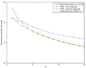
Figure 1: The new bounds on the heavy ball and fast gradient methods.

N Heavy Ball FGM, main FGM, auxiliary Known bound on FGM (4.1) 1 LR²/6.00 LR²/6.00 LR²/2.00 LR²/2.0=2LR²/(1+1)² 2 LR²/7.99 LR²/10.00 LR²/6.00 LR²/4.5=2LR²/(2+1)² 3 LR²/9.00 LR²/15.13 LR²/11.13 LR²/8.0=2LR²/(3+1)² 4 LR²/12.35 LR²/21.35 LR²/17.35 LR²/12.5=2LR²/(4+1)² 5 LR²/16.41 LR²/28.66 LR²/24.66 LR²/18.0=2LR²/(5+1)² 10 LR²/39.63 LR²/81.07 LR²/77.07 LR²/60.5=2LR²/(10+1)² 20 LR²/89.45 LR²/263.65 LR²/259.65 LR²/220.5=2LR²/(20+1)² 40 LR²/188.99 LR²/934.89 LR²/930.89 LR²/840.5=2LR²/(40+1)² 80 LR²/387.91 LR²/3490.22 LR²/3486.22 LR²/3280.5=2LR²/(80+1)² 160 LR²/785.68 LR²/13427.43 LR²/13423.43 LR²/12960.5=2LR²/(160+1)² 500 LR²/2476.11 LR²/127224.44 LR²/127220.32 LR²/125500.5=2LR²/(500+1)² 1000 LR²/4962.01 LR²/504796.99 LR²/504798.28 LR²/501000.5=2LR²/(1000+1)²

Figure 2: The new bounds for HBM and FGM versus the classical bound on Nesterov’s algorithm.

Note that as far as the authors are aware, there is no known convergence rate result for the HBM on the class of convex functions in $C^{1,1}_{L}$. As can be seen from the above results, the numerical bound for HBM behaves slightly better than the gradient method (compare with the explicit bound given in Theorem 3.1), but remains much slower than the fast gradient scheme (FGM).

Considering the results on the FGM, note that the numerical bounds for the main sequence of point $x_{i}$ and the corresponding values at the auxiliary sequence $y_{i}$ of the fast gradient method are very similar and perform slightly better than predicted by the classical bound (4.1). To the best of our knowledge, the complexity of the auxiliary sequence is yet unknown, thus these results encourage us to raise the following conjecture.

Conjecture 4.1.

Let $x_{0},x_{1},\dots$ and $y_{1},y_{2},\dots$ be the main and auxiliary sequences defined by FGM (respectively), then $\{f(x_{i})\}$ and $\{f(y_{i})\}$ converge to the optimal value of the problem with the same rate of convergence.

5 A Best Performing Algorithm: Optimal Step Sizes for The Algorithm Class FO

We now consider the problem of finding the “best” performing algorithm of the form FO with respect to the new bounds. Namely, we consider the problem of minimizing $\operatorname{val}\eqref{P:fopr}$, the optimal value of (Q^′), with respect to the step sizes $h:=(h^{(i)}_{k})_{0\leq k<i\leq N}$ defining the algorithm FO, and which are now considered as unknown variables in FO.

We denote by $\tilde{A}_{i,j}(h)$ and $\tilde{D}_{i}(h)$, the matrices given in (4.3), which are functions of the algorithm step sizes $h$. The resulting bound derived in Proposition 4.2 is thus a function of $h$, and the problem of minimizing $\operatorname{val}\eqref{P:foprd}$ with respect to the step sizes $h$ thus consists of solving the following bilinear problem:

$$\begin{aligned} \min_{h,\lambda,\tau,t}\ \left\{\frac{1}{2}t:\begin{pmatrix}\sum_{i=1}^{N}\lambda_{i}\tilde{A}_{i-1,i}(h)+\sum_{i=0}^{N}\tau_{i}\tilde{D}_{i}(h)&\frac{1}{2}\tau\\ \frac{1}{2}\tau^{T}&\frac{1}{2}t\end{pmatrix}\succeq 0,(\lambda,\tau)\in\tilde{\Lambda}\right\},\end{aligned}$$ (BIL)

with $\tilde{\Lambda}$ defined as in (4.4).

Note that the feasibility of (BIL) follows from the proof of Theorem 3.2, where an explicit feasible point is given to (DG^′), which is a special instance of (BIL) when the steps $(h^{(i)}_{k})$ are chosen as in the gradient method.

From the definition of the matrices $\tilde{A}_{i,j}(h)$ and $\tilde{D}_{i}(h)$, we get

$$\sum_{i=1}^{N}\lambda_{i}\tilde{A}_{i-1,i}(h)+\sum_{i=0}^{N}\tau_{i}\tilde{D}_{i}(h) =\frac{1}{2}\sum_{i=1}^{N}\lambda_{i}(u_{i-1}-u_{i})(u_{i-1}-u_{i})^{T}+\frac{1}{2}\sum_{i=0}^{N}\tau_{i}u_{i}u_{i}^{T}$$

$$\quad+\frac{1}{2}\sum_{i=1}^{N}\sum_{k=0}^{i-1}\left(\lambda_{i}h_{k}^{(i)}+\tau_{i}\sum_{t=k+1}^{i}h_{k}^{(t)}\right)(u_{i}u_{k}^{T}+u_{k}u_{i}^{T}).$$

Introducing the new variables:

$$r_{i,k}=\lambda_{i}h_{k}^{(i)}+\tau_{i}\sum_{t=k+1}^{i}h_{k}^{(t)},\quad i=1,\dots,N,\ k=0,\dots,i-1$$ (5.1)

and denoting $r=(r_{i,k})_{0\leq k<i\leq N}$, we obtain the following linear SDP relaxation of (BIL):

$$\begin{aligned} \min_{r,\lambda,\tau,t}\ \left\{\frac{1}{2}t:\begin{pmatrix}S(r,\lambda,\tau)&\frac{1}{2}\tau\\ \frac{1}{2}\tau^{T}&\frac{1}{2}t\end{pmatrix}\succeq 0,\ (\lambda,\tau)\in\tilde{\Lambda}\right\},\end{aligned}$$ (LIN)

where

$$S(r,\lambda,\tau) =\frac{1}{2}\sum_{i=1}^{N}\lambda_{i}(u_{i-1}-u_{i})(u_{i-1}-u_{i})^{T}+\frac{1}{2}\sum_{i=0}^{N}\tau_{i}u_{i}u_{i}^{T}+\frac{1}{2}\sum_{i=1}^{N}\sum_{k=0}^{i-1}r_{i,k}(u_{i}u_{k}^{T}+u_{k}u_{i}^{T}).$$

This convex SDP can now be efficiently solved by numerical methods. As the following theorem shows, its solution can be used to construct a solution for (BIL) with optimal step sizes $h$.

Theorem 5.1.

Suppose $(r^{\ast},\lambda^{\ast},\tau^{\ast},t^{\ast})$ is an optimal solution for (LIN), then $(h,\lambda^{\ast},\tau^{\ast},t^{\ast})$ is an optimal solution for (BIL), where $h=(h_{k}^{(i)})_{0\leq k<i\leq N}$ is defined by the following recursive rule

$$h_{k}^{(i)}=\begin{cases}\frac{\tau_{i}^{\ast}\sum_{t=k+1}^{i-1}h_{k}^{(t)}-r_{i,k}^{\ast}}{\lambda_{i}^{\ast}}&\lambda_{i}^{\ast}\neq 0\\ 0&\lambda_{i}^{\ast}=0\end{cases},\quad i=1,\dots,N,\ k=0,\dots,i-1.$$ (5.2)

Proof.

As (LIN) is a relaxation of (BIL), it is enough to show that (BIL) can achieve the same objective value. Let $(r^{\ast},\lambda^{\ast},\tau^{\ast},t^{\ast})$ be an optimal solution for (LIN). If $\lambda_{i}^{\ast}\neq 0$ for all $1\leq i\leq N$, then (5.2) satisfies all the equations in (5.1) and therefore $(h,\lambda^{\ast},\tau^{\ast},t^{\ast})$ is feasible for (BIL).

Suppose $\lambda^{\ast}_{m}=0$ for some $1\leq m\leq N$ and that $m$ is the maximal index with this property. Then by the equality and non-negativity constraints in (LIN), we get that $\lambda^{\ast}_{1}=\lambda^{\ast}_{2}=\dots=\lambda^{\ast}_{m}=0$ and $\tau^{\ast}_{0}=\tau^{\ast}_{1}=\dots=\tau^{\ast}_{m-1}=0$. Let $S:=S(r,\lambda^{\ast},\tau^{\ast})$, then by the positive semidefinite constraint in (LIN), we have $S\succeq 0$. From the linear equalities connecting $\lambda$ and $\tau$ it follows that

$$S_{i,i}=\begin{cases}\frac{1}{2}(\lambda_{1}^{\ast}+\tau_{0}^{\ast})=\lambda_{1}^{\ast},&\quad i=1\\ \frac{1}{2}(\lambda_{i}^{\ast}+\lambda_{i-1}^{\ast}+\tau_{i-1}^{\ast})=\lambda_{i}^{\ast},&\quad i=2,\dots,N\end{cases},$$

and we get that $S_{1,1}=\dots=S_{m,m}=0$. By the properties of positive semidefinite matrices we now get that $r_{i,k}^{\ast}=0$ for $i=1,\dots,m$ and $k=0,\dots,i-1$, hence the set of equations (5.1) with the chosen values of $h_{k}^{(i)}$ is consistent. ∎

The optimal value of (LIN) for various values of $N$ is summarized in Figure 3. The resulting new algorithm with the computed optimal step sizes $h_{k}^{(i)}$ is illustrated for $N=5$ and given in Figure 4. As can be seen from these results, (compare with Figure 2) the performance of the new algorithm is almost exactly two times better than the performance of the fast gradient method.

N val(LIN) 1 LR²/8.00 2 LR²/16.16 3 LR²/26.53 4 LR²/39.09 5 LR²/53.80 10 LR²/159.07 20 LR²/525.09 40 LR²/1869.22 80 LR²/6983.13 160 LR²/26864.04 500 LR²/254482.61 1000 LR²/1009628.17

Figure 3: The value of the optimal value of (LIN) for various values of $N$.

$$x_{1}\leftarrow x_{0}+\textstyle\frac{1.6180}{L}f^{\prime}(x_{0})$$

$$x_{2}\leftarrow x_{1}+\textstyle\frac{0.1741}{L}f^{\prime}(x_{0})+\textstyle\frac{2.0194}{L}f^{\prime}(x_{1})$$

$$x_{3}\leftarrow x_{2}+\textstyle\frac{0.0756}{L}f^{\prime}(x_{0})+\textstyle\frac{0.4425}{L}f^{\prime}(x_{1})+\textstyle\frac{2.2317}{L}f^{\prime}(x_{2})$$

$$x_{4}\leftarrow x_{3}+\textstyle\frac{0.0401}{L}f^{\prime}(x_{0})+\textstyle\frac{0.2350}{L}f^{\prime}(x_{1})+\textstyle\frac{0.6541}{L}f^{\prime}(x_{2})+\textstyle\frac{2.3656}{L}f^{\prime}(x_{3})$$

$$x_{5}\leftarrow x_{4}+\textstyle\frac{0.0178}{L}f^{\prime}(x_{0})+\textstyle\frac{0.1040}{L}f^{\prime}(x_{1})+\textstyle\frac{0.2894}{L}f^{\prime}(x_{2})+\textstyle\frac{0.6043}{L}f^{\prime}(x_{3})+\textstyle\frac{2.0778}{L}f^{\prime}(x_{4})$$

Figure 4: A first-order algorithm with optimal step-sizes for $N=5$.

6 Acknowledgements

This work was initiated during our participation to the “Modern Trends in Optimization and Its Application” program at IPAM, (UCLA), September-December 2010. We would like to thank IPAM for their support and for the very pleasant and stimulating environment provided to us during our stay. We would also like to thank Simi Haber, Ido Ben-Eliezer and Rani Hod for their help in the proof of Lemma 3.3.

Appendix A Proof of Lemma 3.3

We now establish the positive definiteness of the matrices $S_{0}$ and $S_{1}$ given in (3.8) and (3.9), respectively.

A.1 $S_{0}\succ 0$

We begin by showing that $S_{0}$ is positive definite. Recall that

$$S_{0}=\begin{pmatrix}2\lambda_{1}&-\lambda_{1}\\ -\lambda_{1}&2\lambda_{2}&-\lambda_{2}\\ &-\lambda_{2}&2\lambda_{3}&-\lambda_{3}\\ &&\ddots&\ddots&\ddots\\ &&&-\lambda_{N-1}&2\lambda_{N}&-\lambda_{N}\\ &&&&-\lambda_{N}&1\\ \end{pmatrix}$$

for

$$\lambda_{i} =\frac{i}{2N+1-i},\qquad i=1,\dots,N.$$

Let us look at $x^{T}S_{0}x$ for any $x=(x_{0},\dots,x_{N})^{T}$:

$$x^{T}S_{0}x =\sum_{i=0}^{N-1}2\lambda_{i+1}x_{i}^{2}-2\sum_{i=0}^{N-1}\lambda_{i+1}x_{i}x_{i+1}+x_{N}^{2}$$

$$=\sum_{i=0}^{N-1}\lambda_{i+1}(x_{i+1}-x_{i})^{2}+\lambda_{1}x_{0}^{2}+\sum_{i=1}^{N-1}(\lambda_{i+1}-\lambda_{i})x_{i}^{2}+(1-\lambda_{N})x_{N}^{2}$$

which is always positive for $x\neq 0$. We conclude that $S_{0}$ is positive definite.

A.2 $S_{1}\succ 0$

We will show that $S_{1}$ is positive definite using Sylvester’s criterion.

Recall that

$$S_{1}=\begin{pmatrix}2\lambda_{1}&\lambda_{2}-\lambda_{1}&\dots&\lambda_{N}-\lambda_{N-1}&1-\lambda_{N}\\ \lambda_{2}-\lambda_{1}&2\lambda_{2}&&\lambda_{N}-\lambda_{N-1}&1-\lambda_{N}\\ \vdots&&\ddots&&\vdots\\ \lambda_{N}-\lambda_{N-1}&\lambda_{N}-\lambda_{N-1}&&2\lambda_{N}&1-\lambda_{N}\\ 1-\lambda_{N}&1-\lambda_{N}&\dots&1-\lambda_{N}&1\\ \end{pmatrix}$$

for

$$\lambda_{i} =\frac{i}{2N+1-i},\qquad i=1,\dots,N.$$

A recursive expression for the determinants

We begin by deriving a recursion rule for the determinant of matrices of the following form:

$$M_{k}=\begin{pmatrix}d_{0}&a_{1}&a_{2}&\dots&a_{k-1}&a_{k}\\ a_{1}&d_{1}&a_{2}&&a_{k-1}&a_{k}\\ a_{2}&a_{2}&d_{2}&&a_{k-1}&a_{k}\\ \vdots&&&\ddots&&\vdots\\ a_{k-1}&a_{k-1}&a_{k-1}&&d_{k-1}&a_{k}\\ a_{k}&a_{k}&a_{k}&\dots&a_{k}&d_{k}\end{pmatrix}.$$

To find the determinant of $M_{k}$, subtract the one before last row multiplied by $\frac{a_{k}}{a_{k-1}}$ from the last row: the last row becomes

$$(0,\dots,0,a_{k}-\frac{a_{k}}{a_{k-1}}d_{k-1},d_{k}-\frac{a_{k}}{a_{k-1}}a_{k}).$$

Expanding the determinant along the last row we get

$$\det M_{k}=(d_{k}-\frac{a_{k}}{a_{k-1}}a_{k})\det M_{k-1}-(a_{k}-\frac{a_{k}}{a_{k-1}}d_{k-1})\det(M_{k})_{k,k-1}$$

where $(M_{k})_{k,k-1}$ denotes the $k,k-1$ minor:

$$(M_{k})_{k,k-1}=\begin{pmatrix}d_{0}&a_{1}&a_{2}&\dots&a_{k-2}&a_{k}\\ a_{1}&d_{1}&a_{2}&&a_{k-2}&a_{k}\\ a_{2}&a_{2}&d_{2}&&a_{k-2}&a_{k}\\ \vdots&&&\ddots\\ a_{k-2}&a_{k-2}&a_{k-2}&&d_{k-2}&a_{k}\\ a_{k-1}&a_{k-1}&a_{k-1}&&a_{k-1}&a_{k}\end{pmatrix}.$$

If we multiply the last column of $(M_{k})_{k,k-1}$ by $\frac{a_{k-1}}{a_{k}}$ we get a matrix that is different from $M_{k-1}$ by only the corner element. Thus by basic determinant properties we get that

$$\frac{a_{k-1}}{a_{k}}\det(M_{k})_{k,k-1}=\det M_{k-1}+(a_{k-1}-d_{k-1})\det M_{k-2}.$$

Combining these two results, we have found the following recursion rule for $\det M_{k}$, $k\geq 2$:

$$\det M_{k}=(d_{k}-\frac{a_{k}}{a_{k-1}}a_{k})\det M_{k-1}$$

$$\qquad-(a_{k}-\frac{a_{k}}{a_{k-1}}d_{k-1})\left(\frac{a_{k}}{a_{k-1}}\det M_{k-1}+(a_{k}-\frac{a_{k}}{a_{k-1}}d_{k-1})\det M_{k-2}\right)$$

$$=\left((d_{k}-\frac{a_{k}}{a_{k-1}}a_{k})-(a_{k}-\frac{a_{k}}{a_{k-1}}d_{k-1})\frac{a_{k}}{a_{k-1}}\right)\det M_{k-1}-\left(a_{k}-\frac{a_{k}}{a_{k-1}}d_{k-1}\right)^{2}\det M_{k-2}$$

or

$$\det M_{k}=\left(d_{k}-\frac{2a_{k}^{2}}{a_{k-1}}+\frac{a_{k}^{2}d_{k-1}}{a_{k-1}^{2}}\right)\det M_{k-1}-a_{k}^{2}\left(1-\frac{d_{k-1}}{a_{k-1}}\right)^{2}\det M_{k-2}.$$ (A.1)

Obviously, the recursion base cases are given by

$$\det M_{0}=d_{0},$$

$$\det M_{1}=d_{0}d_{1}-a_{1}^{2}.$$

Closed form expressions for the determinants

Going back to our matrix, $S_{1}$, by choosing

$$d_{i}=2\frac{i+1}{2N-i},\quad i=0,\dots,N-1$$

$$d_{N}=1$$

$$a_{i}=\frac{i+1}{2N-i}-\frac{i}{2N+1-i},\quad i=1,\dots,N-1$$

$$a_{N}=1-\frac{N}{N+1}=\frac{1}{N+1},$$

we get that $M_{k}$ is the $k+1$’th leading principal minor of the matrix $S_{1}$. The recursion rule (A.1) can now be solved for this choice of $a_{i}$ and $d_{i}$. The solution is given by:

$$\det M_{k}= \frac{(2N+1)^{2}}{(2N-k)^{2}}\left(1+\sum_{i=0}^{k}\frac{2N-2k-1}{2N+4Ni-2i^{2}+1}\right)\prod_{i=0}^{k}\frac{2N+4Ni-2i^{2}+1}{(2N+1-i)^{2}},$$ (A.2)

for $k=0,\dots,N-1$, and

$$\det M_{N}=\det L_{1}= \frac{(2N+1)^{2}}{(N+1)^{2}}\prod_{i=0}^{N-1}\frac{2N+4Ni-2i^{2}+1}{(2N+1-i)^{2}}.$$ (A.3)

Verification

We now proceed to verify the expressions (A.2) and (A.3) given above. We will show that these expressions satisfy the recursion rule (A.1) and the base cases of the problem. We begin by verifying the base cases:

$$\det M_{0} =\frac{(2N+1)^{2}}{(2N)^{2}}\left(1+\frac{2N-1}{2N+1}\right)\frac{1}{2N+1}=\frac{1}{N}=d_{0},$$

$$\det M_{1} =\frac{(2N+1)^{2}}{(2N-1)^{2}}\left(1+\frac{2N-3}{2N+1}+\frac{2N-3}{6N-1}\right)\frac{1}{2N+1}\frac{6N-1}{(2N)^{2}}$$

$$=\frac{28N^{2}-20N-1}{4N^{2}(2N-1)^{2}}=\frac{4}{N(2N-1)}-\left(\frac{2}{2N-1}-\frac{1}{2N}\right)^{2}=d_{0}d_{1}-a_{1}^{2}.$$

Now suppose $2\leq k\leq N$. Denote

$$\alpha_{k} =d_{k}-\frac{2a_{k}^{2}}{a_{k-1}}+\frac{a_{k}^{2}d_{k-1}}{a_{k-1}^{2}}$$

$$=\begin{cases}4\frac{(2N+1)k-k^{2}-1}{(2N-k)^{2}},&k<N\\ 3\frac{2N^{2}+2N-1}{(2N+1)^{2}},&k=N\end{cases}$$

$$\beta_{k} =a_{k}^{2}\left(1-\frac{d_{k-1}}{a_{k-1}}\right)^{2}$$

$$=\begin{cases}\frac{(4kN-2N-2k^{2}+4k-1)^{2}}{(2N-k)^{2}(2N-k+1)^{2}},&k<N\\ \frac{(2N^{2}+2N-1)^{2}}{(N+1)^{2}(2N+1)^{2}},&k=N\end{cases},$$

then the recursion rule (A.1) can be written as

$$\det M_{k}=\alpha_{k}\det M_{k-1}-\beta_{k}\det M_{k-2}.$$

Further denote

$$f_{i} =\frac{(2N+1)^{2}}{(2N-i)^{2}},\quad i=0,\dots,N-1,$$

$$g_{i} =2N-2i-1,\quad i=0,\dots,N-1,$$

$$x_{i} =\frac{1}{2N+4Ni-2i^{2}+1},\quad i=0,\dots,N-1,$$

$$y_{i} =\frac{2N+4Ni-2i^{2}+1}{(2N+1-i)^{2}},\quad i=0,\dots,N-1,$$

then the solution (A.2) becomes

$$\det M_{k}= f_{k}\left(1+g_{k}\sum_{i=0}^{k}x_{i}\right)\prod_{i=0}^{k}y_{i},$$

and (A.3) becomes

$$\det M_{N}= \frac{(2N+1)^{2}}{(N+1)^{2}}\prod_{i=0}^{N-1}y_{i}.$$

Substituting (A.2) in the RHS of (A.1) we get that for $k=2,\dots,N$

$$\alpha_{k}\det M_{k-1}-\beta_{k}\det M_{k-2}$$

$$=\alpha_{k}f_{k-1}\left(1+g_{k-1}\sum_{i=0}^{k-1}x_{i}\right)\prod_{i=0}^{k-1}y_{i}-\beta_{k}f_{k-2}\left(1+g_{k-2}\sum_{i=0}^{k-2}x_{i}\right)\prod_{i=0}^{k-2}y_{i}$$

$$=\left(\alpha_{k}f_{k-1}\left(1+g_{k-1}x_{k-1}+g_{k-1}\sum_{i=0}^{k-2}x_{i}\right)-\frac{\beta_{k}}{y_{k-1}}f_{k-2}-\frac{\beta_{k}}{y_{k-1}}f_{k-2}g_{k-2}\sum_{i=0}^{k-2}x_{i}\right)\prod_{i=0}^{k-1}y_{i}$$

$$=\left(\alpha_{k}f_{k-1}(1+g_{k-1}x_{k-1})-\frac{\beta_{k}}{y_{k-1}}f_{k-2}+\left(\alpha_{k}f_{k-1}g_{k-1}-\frac{\beta_{k}}{y_{k-1}}f_{k-2}g_{k-2}\right)\sum_{i=0}^{k-2}x_{i}\right)\prod_{i=0}^{k-1}y_{i}.$$

It is straightforward (although somewhat involved) to verify that for $k<N$

$$\alpha_{k}f_{k-1}(1+g_{k-1}x_{k-1})-\frac{\beta_{k}}{y_{k-1}}f_{k-2}=f_{k}y_{k}(1+g_{k}x_{k-1}+g_{k}x_{k}),$$

and

$$\alpha_{k}f_{k-1}g_{k-1}-\frac{\beta_{k}}{y_{k-1}}f_{k-2}g_{k-2}=f_{k}g_{k}y_{k}.$$

We therefore get

$$\alpha_{k}\det M_{k-1}-\beta_{k}\det M_{k-2}$$

$$=\left(f_{k}y_{k}(1+g_{k}x_{k-1}+g_{k}x_{k})+f_{k}g_{k}y_{k}\sum_{i=0}^{k-2}x_{i}\right)\prod_{i=0}^{k-1}y_{i}$$

$$=f_{k}\left(1+g_{k}\sum_{i=0}^{k}x_{i}\right)\prod_{i=0}^{k}y_{i}$$

$$=\det M_{k},$$

and thus (A.2) satisfies (A.1). It is also possible to show that

$$\alpha_{N}f_{N-1}(1+g_{N-1}x_{N-1})-\frac{\beta_{N}}{y_{N-1}}f_{N-2}=\frac{(2N+1)^{2}}{(N+1)^{2}},$$

$$\alpha_{N}f_{N-1}g_{N-1}-\frac{\beta_{N}}{y_{N-1}}f_{N-2}g_{N-2}=0,$$

thus, for $k=N$

$$\alpha_{N}\det M_{N-1}-\beta_{N}\det M_{N-2}$$

$$=\frac{(2N+1)^{2}}{(N+1)^{2}}\prod_{i=0}^{N-1}y_{i}$$

$$=\det M_{N},$$

and the expression (A.3) is also verified.

To complete the proof, note that the closed form expressions for $\det M_{k}$ consist of sums and products of positive values, hence $\det M_{k}$ is positive, and thus follows from Sylvester’s criterion that $S_{1}$ is positive definite.

References

• [1] H. Attouch, J. Bolte, and P. Redont. Optimizing properties of an inertial dynamical system with geometric damping. Link with proximal methods. Control Cybernet., 31(3):643–657, 2002. Well-posedness in optimization and related topics (Warsaw, 2001).
• [2] H. Attouch, X. Goudou, and P. Redont. The heavy ball with friction method. I. The continuous dynamical system: global exploration of the local minima of a real-valued function by asymptotic analysis of a dissipative dynamical system. Commun. Contemp. Math., 2(1):1–34, 2000.
• [3] A. Beck. Quadratic matrix programming. SIAM J. Optim., 17(4):1224–1238, 2006.
• [4] A. Beck and M. Teboulle. A fast iterative shrinkage-thresholding algorithm for linear inverse problems. SIAM J. Img. Sci., 2:183–202, March 2009.
• [5] A. Beck and M. Teboulle. Gradient-based algorithms with applications to signal-recovery problems. In Convex optimization in signal processing and communications, pages 42–88. Cambridge Univ. Press, Cambridge, 2010.
• [6] A. Ben-Tal and A. S. Nemirovskii. Lectures on modern convex optimization. Siam, 2001.
• [7] S. Boyd and L. Vandenberghe. Convex Optimization. Cambridge University Press, March 2004.
• [8] M. Grant and S. Boyd. Graph implementations for nonsmooth convex programs. In V. Blondel, S. Boyd, and H. Kimura, editors, Recent Advances in Learning and Control, Lecture Notes in Control and Information Sciences, pages 95–110. Springer-Verlag Limited, 2008. http://stanford.edu/~boyd/graph_dcp.html.
• [9] M. Grant and S. Boyd. CVX: Matlab software for disciplined convex programming, version 1.21. http://cvxr.com/cvx, April 2011.
• [10] C. Helmberg, F. Rendl, R. Vanderbei, and H. Wolkowicz. An interior-point method for semidefinite programming. SIAM J. Optim., 6:342–361, 1996.
• [11] J. J. Moreau. Proximité et dualité dans un espace hilbertien. Bull. Soc. Math. France, 93:273–299, 1965.
• [12] A. S. Nemirovsky and D. B. Yudin. Problem complexity and method efficiency in optimization. A Wiley-Interscience Publication. John Wiley & Sons Inc., New York, 1983. Translated from the Russian and with a preface by E. R. Dawson, Wiley-Interscience Series in Discrete Mathematics.
• [13] Yu. Nesterov. A method of solving a convex programming problem with convergence rate O$(1/k^{2})$. Soviet Mathematics Doklady, 27(2):372–376, 1983.
• [14] Yu. Nesterov. Introductory lectures on convex optimization: a basic course. Applied optimization. Kluwer Academic Publishers, 2004.
• [15] D. P. Palomar and Y. C. Eldar, editors. Convex Optimization in Signal Processing and Communications. Cambridge University Press, 2010.
• [16] B. T. Polyak. Some methods of speeding up the convergence of iteration methods. USSR Comp. Math. Math. Phys., 4(5):1–17, 1964.
• [17] R. T. Rockafellar and J. B. W. Roger. Variational analysis, volume 317 of Grundlehren der Mathematischen Wissenschaften [Fundamental Principles of Mathematical Sciences]. Springer-Verlag, Berlin, 1998.
• [18] S. Sra, S. Nowozin, and S. J. Wright, editors. Optimization for Machine Learning. MIT Press, Cambridge, MA., 2011.
• [19] L. Vandenberghe and S. Boyd. Semidefinite programming. SIAM Rev., 38(1):49–95, 1996.