Non-Gaussian statistics and extreme waves in a nonlinear optical cavity

Abstract

A unidirectional optical oscillator is built by using a liquid crystal light-valve that couples a pump beam with the modes of a nearly spherical cavity. For sufficiently high pump intensity, the cavity field presents a complex spatio-temporal dynamics, accompanied by the emission of extreme waves and large deviations from the Gaussian statistics. We identify a mechanism of spatial symmetry breaking, due to a hypercycle-type amplification through the nonlocal coupling of the cavity field.

Extreme waves are anomalously large amplitude phenomena developing suddenly out of normal waves, living for a short time and appearing erratically with a small probability. These rare and extreme events have been observed since long time on the ocean surfaces oceanography , and, in this context, have been called freak or rogue waves. Recently, rogue waves have been reported in an optical experiment Solli and in acoustic turbulence in He II McClintock . Associated with extreme waves are L-shaped statistics, with a probability of large peak occurrence much larger than predicted by Gaussian statistics. Different mechanisms to explain the origin of extreme waves have been proposed, including nonlinear focusing via modulational instability (MI) Onorato and focusing of line currents White . In optical fibers, numerical simulations of the nonlinear Schrödinger equation (NLSE) Dudley have established a direct analogy between optical and water rogue waves. In a spatially extended system, the formation of large amplitude and localized pulses, so-called optical needles, has been evidenced by numerical simulations for transparent media with saturating self-focusing nonlinearity Rosanov . Similar space-time phenomena, such as collapsing filaments, are also predicted in optical wave turbulence Dyachenko . Recently, the spatio-temporal dynamics of MI-induced bright optical spots was observed in Ref. Shih and an algebraic power spectrum tail was reported due to momentum cascade Dylov . Nevertheless, no experimental evidence has been given up to now of extreme waves in a spatially extended optical system.

Here, we report, what is, at our knowledge, the first experimental evidence of extreme waves and non-Gaussian statistics in a 2D spatially extended optical system. The experiment consists of a nonlinear optical cavity, formed by a unidirectional ring oscillator with a liquid crystal light-valve (LCLV) as the gain medium. While for low pump the amplitude follows a Gaussian statistics, for sufficiently high pump we observe large deviations from Gaussianity, accompanied by the emission of extreme waves that appear on the transverse profile of the optical beam as genuine spatiotemporal phenomena, developing erratically in time and in space. The observations are confirmed by numerical simulation of the full model equations. Moreover, by introducing a mean-field simplified model, we show that extreme waves in the cavity are generated by a novel mechanism, which is based on a hypercycle-type amplification hypercycle occurring via nonlocal coupling of different spatial regions.

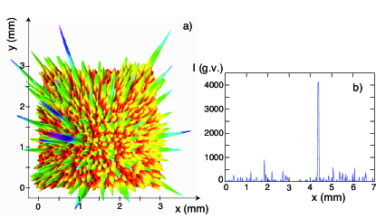
Figure 1: (color online). a) Instantaneous experimental profile of the transverse intensity distribution; b) a 1-D profile showing an extreme event; $I$ is measured in gray values, g.v.

The experimental setup is essentially the one described in ourprl . The ring cavity is formed by three high-reflectivity dielectric mirrors and a lens of $f=70$ $cm$ focal length. The total cavity length is $L=273.3$ $cm$ and the lens is positioned at a distance $L_{1}=88.1$ $cm$ from the entrance plane of the LCLV. The coordinate system is taken such that $z$ is along the cavity axis and $x,y$ are on the transverse plane. A LCLV supplies the gain through a two-wave mixing process IOP that couples the pump beam with the cavity modes. The LCLV is made of a nematic liquid crystal layer, thickness $d=14$ $\mu m$, inserted in between a glass wall and a thin slice $20$x$30$x$1$ $mm^{3}$ of the photoconductive $B_{12}SiO_{20}$ (BSO) crystal. A voltage $V_{0}$ is applied by means of transparent electrodes. The working point is fixed at $V_{0}\simeq 20.3$ $V$, frequency $75$ $Hz$. The LCLV is pumped by an enlarged and collimated ($10$ $mm$ diameter) beam from a solid state diode pumped laser ($\lambda=532$ $nm$), linearly polarized in the same direction of the liquid crystal nematic director. The pump and the cavity field, $E_{p}$ and, respectively, $E_{c}$, are polarized in the same direction and have a frequency difference of a few $Hz$, the detuning being selected by the voltage $V_{0}$ applied to the LCLV ourPRA .

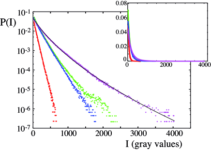
Figure 2: (color online) Experimental PDF of the cavity field intensity; the pump is varied from $I_{p}/I_{th}=1.8$ (red), $4.0$ (blue), $4.2$ (green) and $6.4$ (purple). The red distribution is practically exponential. The black line is the stretched exponential function that fits the purple distribution, with $c_{1}=29.5$. The inset shows the L-shape of the PDF in the linear scale.

A small fraction ($4\%$) of the cavity field is extracted by a beam sampler and sent to a CCD camera ($1024$x$768$ pixels and $12$ bits depth). The detection optical path is set so that the camera records the same field distribution as in the entrance plane of the LCLV. The Fresnel number is fixed to $F=130$ and can be carefully controlled through a spatial filter introduced near the lens.

For relatively low pump intensity, $I_{p}=|E_{p}|^{2}=2.0$ $mW/cm^{2}$, the cavity field shows a complex spatio-temporal dynamics, with the formation of many uncorrelated domains. At larger pump, extreme events appear as large amplitude peaks, standing over a speckle-like background. An instantaneous experimental profile of the transverse intensity distribution for $I_{p}=4.2$ $mW/cm^{2}$, is shown in Fig.1. In the inset the 1-D profile shows a large event. Note the difference of the peak amplitude with respect to the background values of the intensity. The locations of the large peaks change spontaneously in time. The typical time-scale of the dynamical evolution is $100$ $ms$, which is ruled by the response time of the liquid crystals DeGennes .

The probability density functions (PDF) of the light intensity are determined experimentally by acquiring a large set of images (about one thousand) and then performing the histograms of the intensity values on the whole image stack. In Fig.2 the PDF of the cavity field intensity, $I=|E_{c}|^{2}$, are displayed for different values of the pump, $I_{p}/I_{th}=1.8$, $4.0$, $4.2$ and $6.4$, $I_{th}=1.2$ $mW/cm^{2}$ being the threshold for optical oscillations. The dark probability $P(I=0)$ is the same for all the pump intensities. The log-linear plots in Fig.2 reveal increasingly large deviations from the exponential behavior as we increase the pump intensity. All the distributions are well fitted by the stretched exponential function $Ne^{-\sqrt{c_{1}+c_{2}I}}$, $1/c_{1}$ providing a measure of the deviation from the exponential function. The black line is the fitting function of the PDF with $I_{p}/I_{th}=6.4$. The fit is performed by setting the mean intensity and the variance of the fitting function equal to the experimental values.

Note that an exponential statistics for the intensity corresponds to a Gaussian statistics for the field amplitude. Therefore, an exponential intensity PDF is characteristic of a speckles pattern, where each point receive the uncorrelated contributions of many uncoupled modes. At low pump, this is indeed the behavior displayed by the cavity field. However, when the pump increases, the increasing nonlinear coupling leads to a complex space-time dynamics and extreme events populate the tails of the PDF, providing a large deviation from Gaussianity. The L-shape of the statistics is clearly visible in the inset of Fig.2, where the PDF are plotted in linear scale.

To perform numerical simulations, we have considered the full model equations developed in Ref. ourPRA

$${\partial n_{0}\over\partial t} = -n_{0}+\alpha|E_{c}|^{2},$$ (1)

$${\partial n_{1}\over\partial t} = -n_{1}+\alpha E_{c}E_{p}^{*},$$

where $n_{0}$ and $n_{1}$ are, respectively, the amplitude of the homogeneous refractive index and the amplitude of the refractive index grating at the spatial frequency $k_{c}-k_{p}$, $k_{c}$ and $k_{p}$ being the optical wave numbers of the pump and cavity field. $\alpha$ is the nonlinear coefficient of the LCLV, and we have neglected the diffusion length due to elastic coupling in the liquid crystal. The dynamics of the liquid crystals is much slower than the settling of the cavity field, thus $E_{c}$ follows adiabatically the evolution of $n_{0}$ and $n_{1}$. Then, by taking the wave propagation equation with the cavity boundary conditions, we obtain that

$$E_{c}=i\sum_{k=0}^{\infty}{[\hat{C}e^{in_{0}}J_{0}(2|n_{1}|)]^{k}}\hat{C}e^{in_{0}}{n_{1}\over|n_{1}|}J_{1}(2|n_{1}|)E_{p},$$ (2)

where $J_{m}$ is the Bessel function of the first kind and of order $m$, and $\hat{C}$ is an operator accounting for the geometry of the cavity and losses, $\hat{C}=\Gamma^{1/2}e^{i\delta}\hat{S}_{x}e^{i(L_{0}\nabla_{\perp}^{2}/2k_{p})}e^{-i(k_{p}\vec{r}_{\perp}^{2}/2f)}e^{i(L_{1}\nabla_{\perp}^{2}/2k_{p})}$, with $1-\Gamma$ the photon losses, $L_{0}\equiv L-L_{1}$ and $\delta$ the phase retardation in a round-trip. $\hat{S}_{x}$ is a symmetry operator that inverts the $x$ axis, thus accounting for the odd number of mirrors, $\nabla_{\perp}^{2}$ is the transverse Laplacian and $\vec{r}_{\perp}$ the position in the transverse $(x,y)$ plane.

For the numerical convenience, $\hat{C}$ has been implemented by using an equivalent nearly plane cavity with the $y$-axis inversion $\hat{S}_{y}$ and two lenses just before and after the LCLV Siegman . In order to account for the finite size of the LCLV and the diaphragm inserted near the lens, we have used in the simulations a diaphragm both in the space and in the Fourier plane. In particular, we have used a spatial filter with radius equal to $0.4$ $cm$ and a Fourier filter with radius $k=3.2\cdot 10^{-3}k_{p}$ . For the other parameters, we have set the liquid crystal response time $\tau=0.1$ $s$, the photon loss fraction $1-\Gamma$ between $0.7$ and $0.8$, and $\alpha$ is chosen in such a way that the intensity unit is the pump threshold for the activation of the cavity field.

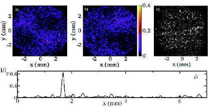
Figure 3: (color online) a) b) Numerical snapshots of the cavity field intensity at two different instant times; $I_{p}=8$, $1-\Gamma=0.7$; c) experimental snapshot of the cavity field, $I_{p}/I_{th}=4.0$. d) 1D section of a 2D numerical intensity distribution.

Starting with a random initial condition, we observe a transient speckle-like behavior, then a breaking of the $y\leftrightarrow-y$ inversion symmetry occurs and the coarse-grained intensity distribution $|E_{c}(x,y)|^{2}$ becomes non-homogeneous along the $y$ axis. In Fig.3 we report two snapshots of the cavity field intensity $|E_{c}|^{2}$ numerically calculated for $I_{p}=8$, $1-\Gamma=0.7$ and displayed at different instant times. In Fig.3a we can note two large dark (bright) regions symmetrically distributed around the center, while in Fig.3b the left pair has disappeared and the other one is inverted. Typically, the cavity field shows a dynamical evolution with the succession of different spatial configurations, each living for a few seconds. For comparison, we display in Fig.3c an experimental snapshot recorded for $I_{p}/I_{th}=4.0$. In Fig.3d, we report a one-dimensional section of the numerical intensity distribution at another instant time, exhibiting a very large narrow peak in a bright region. Its spatial size is larger than the experimental value because of a narrower spectral filtering that limits, for computational convenience, the number of numerical lattice points.

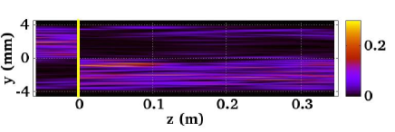
Figure 4: (color online) Cavity field intensity in the $y-z$ plane; the yellow vertical line at $z=0$ indicates the position of the LCLV; $I_{p}=10$, $1-\Gamma=0.7$.

In Fig.4 we have plotted the numerical intensity $|E_{c}|^{2}$ in the $z-y$ plane. The yellow line at $z=0$ represents the position of the LCLV inside the cavity. In the plot, there is clear evidence of both the dynamical symmetry breaking of the intensity profile along $y$ and of the $y$-axis inversion between the impinging and outgoing fields (at left and right of the yellow line, respectively), consistent with the geometry of the experimental cavity, which is nearly spherical and made of an odd number of mirrors. This inversion induces a nonlocal coupling between different spatial regions of the field, thus triggering the hypercycle amplification process that is essential for the symmetry breaking and the long tail statistics. Indeed, we have checked that simulations with a non-inverting nearly plane cavity generate an exponential statistics.

As a consequence of the spatial symmetry breaking, the field exhibits large deviations from Gaussianity. The numerical PDF of the cavity field intensity are displayed in Fig.5 for different values of the pump. The intensities are rescaled in such a way that the PDF have the same value and slope at the origin. The distributions are well fitted by the stretched exponential function $N\exp(-\sqrt{c_{1}+c_{2}I})$ (black dotted lines) and their tails are increasingly populated as the pump increases, in agreement with the experimental observations. The simulations show also that the symmetry breaking is stronger for high cavity losses. Moreover, for the used parameters, the refractive index $n_{0}$ is about four times less than $n_{1}$. The role of $n_{0}$ is to adjust the global phase detuning $\delta$, but it has no effect on the PDF, as we have verified by removing it from the model. Thus, in the following we take $n_{0}$ constant and $1-\Gamma\ll 1$.

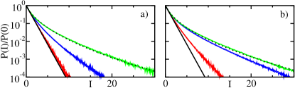
Figure 5: (color online) Numerical PDF of the cavity field intensity for $1-\Gamma=0.7$ (a), $1-\Gamma=0.8$ (b) and different values of the pump: $I_{p}/I_{th}=6$ (blue), $8$ (red), $10$ (green). The black straight and dotted lines are respectively $\exp(-I)$ and $N\exp(-\sqrt{c_{1}+c_{2}I})$, where $N$ and $c_{i}$ are set in order to fit the green distribution; (a) $c_{1}=3.73$, (b) $c_{1}=2.83$.

The $y$ axis inversion (Fig.4) introduces a nonlocal coupling between different space domains with loops of amplification, a mechanism similar to the hyper-cycle chain of reactions in the catalytic processes hypercycle . Because of this mechanism, there is a sort of focusing, for which at some space locations the cavity field grows much more with respect to the surrounding places, giving rise to large amplitude peaks and, hence, to large deviations from the Gaussian statistics. The peaks last a few seconds, after that the hyper-cycle readjusts over new field configurations, yielding new peaks in other space locations.

To elucidate this mechanism we derive a simple two-mode model, where only the evolution of the average refractive index $n_{1}$ is kept, the average being performed over the transverse plane. For a nearly plane cavity, $\bar{n}_{1}$ satisfies approximatively the equation $\tau{d\bar{n}_{1}\over dt}=-\bar{n}_{1}+I_{p}F(\bar{n}_{1})$, where the first and second terms at the r.h.s. account respectively for the liquid crystal relaxation and the grating feeding provided by the pump and cavity fields. As an ansatz for the function $F$, we take a cubic function, which describes a linear growth followed by saturation, due to multiple scattering and pump depletionourPRA .

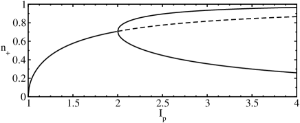
Figure 6: The refractive index $n_{+}$ as a function of $I_{p}$.

When the nearly plane cavity is replaced by a nearly spherical one, the above mean-field picture is modified by the nonlocal coupling due to the $y\leftrightarrow-y$ inversion. We thus have to consider two mean fields $\bar{n}_{+}$ and $\bar{n}_{-}$, where the averages are performed over the upper and lower half-planes, respectively. Accounting for the inversion $y\rightarrow-y$ of the cavity field, we have that, after a round trip, the grating $\bar{n}_{\pm}$ is fed by the grating $\bar{n}_{\mp}$ at the opposite side, i.e, the equation for $\bar{n}$ is replaced by the two following ones for $\bar{n}_{\pm}$,

$$\tau{\partial{\bar{n}}_{\pm}\over\partial t}=-\bar{n}_{\pm}+I_{p}F(\bar{n}_{\mp}),$$ (3)

where we have assumed implicitly that the cavity losses are very high, i.e., the cavity field is negligible after more than one round trip.

The above equations are similar to a hypercycle model for two autocatalytic systems. The main features of $F$ can be captured by the cubic function $F(\bar{n}_{\pm})=\bar{n}_{\pm}-\bar{n}_{\pm}^{3}$. It is easy to show that for $1<I_{p}<2$, Eqs.(3) have only one stable solution, $\bar{n}_{-}=\bar{n}_{+}=0$, whereas for $I_{p}\geq 2$ a bifurcation occurs with the birth of the two stable asymmetric states $n_{+}=2^{-\frac{1}{2}}[1\pm(I_{p}^{2}-4)^{\frac{1}{2}}/I_{p}]^{\frac{1}{2}}$, $n_{-}=2^{-\frac{1}{2}}[1\mp(I_{p}^{2}-4)^{\frac{1}{2}}/I_{p}]^{\frac{1}{2}}$, which break the $y\leftrightarrow-y$ symmetry, thus qualitatively accounting for the experimental and numerical observations. The bifurcation diagram of $\bar{n}_{+}$ is plotted in Fig.6 as function of the pump intensity $I_{p}$. The experimental and numerical bifurcation intensity is about $4$, rather than $2$. This discrepancy is mainly due to the approximation of $F(\bar{n}_{\pm})$ with a cubic function.

In conclusion, we have shown experimentally and numerically that extreme waves arise in a spatially extended nonlinear optical system. We have derived a simplified mean-field model, showing that a spatial symmetry breaking is induced by a nonlocal coupling of the cavity field, which is responsible for a hyper-cycle type amplification of the field and leads to a non-Gaussian statistics.

U.B. and S.R. acknowledge the financial support of the ANR-07- BLAN-0246-03, turbonde. A.M. and F.T.A. acknowledge the financial support of Ente Cassa di Risparmio di Firenze under the project ”dinamiche cerebrali caotiche”.

References

- (1) P. Muller, C. Garrett, and A. Osborne, Oceanography 18, 6 (2005).
- (2) D.R. Solli, et al., Nature 450, 1054 (2007).
- (3) A.N. Ganshin, et al., Phys. Rev. Lett. 101, 065303 (2008).
- (4) M. Onorato, A. R. Osborne, and M. Serio, Phys. Rev. Lett. 96, 014503 (2006).
- (5) B.S. White, B. Fornberg, J. Fluid Mech. 355, 113 (1998).
- (6) J.M. Dudley, G. Genty, and B. Eggleton, Opt. Expr. 16, 3644 (2008).
- (7) N.N. Rosanov, V.E Semenov, and N.V. Vyssotina, J. Opt. B: Quantum Semiclass. Opt. 3, 96 (2001).
- (8) S. Dyachenko, et al., Physica D 57, 96 (1992).
- (9) M.-F. Shih, et al., Phys. Rev. Lett. 88, 133902 (2002).
- (10) D. V. Dylov, J. W. Fleischer, Phys. Rev. A 78, 061804(R) (2008).
- (11) M. Eigen, and P. Schuster, The Hypercycle: A principle of natural self-organization, (Springer, Berlin, 1979).
- (12) U. Bortolozzo, et al., Phys. Rev. Lett. 99, 023901 (2007).
- (13) U. Bortolozzo, S. Residori, and J. P. Huignard, J. Phys. D : Appl. Phys. 41, 224007 (2008).
- (14) A. Montina, et al., Phys. Rev. A 76, 033826 (2007).
- (15) P.G. De Gennes and J. Prost, The Physics of Liquid Crystals, (Oxford Science Publications, Clarendon Press, second edition, 1993).
- (16) A.E. Siegman, Lasers, (University Science Books, 1986).