Numerical renormalization group calculation of impurity internal energy and specific heat of quantum impurity models

Abstract

We introduce a method to obtain the specific heat of quantum impurity models via a direct calculation of the impurity internal energy requiring only the evaluation of local quantities within a single numerical renormalization group (NRG) calculation for the total system. For the Anderson impurity model, we show that the impurity internal energy can be expressed as a sum of purely local static correlation functions and a term that involves also the impurity Green function. The temperature dependence of the latter can be neglected in many cases, thereby allowing the impurity specific heat, $C_{\rm imp}$, to be calculated accurately from local static correlation functions; specifically via $C_{\rm imp}=\frac{\partial E_{\rm ionic}}{\partial T}+\frac{1}{2}\frac{\partial E_{\rm hyb}}{\partial T}$, where $E_{\rm ionic}$ and $E_{\rm hyb}$ are the energies of the (embedded) impurity and the hybridization energy, respectively. The term involving the Green function can also be evaluated in cases where its temperature dependence is non-negligible, adding an extra term to $C_{\rm imp}$. For the non-degenerate Anderson impurity model, we show by comparison with exact Bethe ansatz calculations that the results recover accurately both the Kondo induced peak in the specific heat at low temperatures as well as the high temperature peak due to the resonant level. The approach applies to multiorbital and multichannel Anderson impurity models with arbitrary local Coulomb interactions. An application to the Ohmic two state system and the anisotropic Kondo model is also given, with comparisons to Bethe ansatz calculations. The approach could also be of interest within other impurity solvers, for example, within quantum Monte Carlo techniques.

I Introduction

Quantum impurity models play an important role in condensed matter physics, for example, as models of transition metal and rare-earth impurities in metals Hewson (1997) or two-level systems Zawadowski (1980); Caldeira and Leggett (1983); Leggett et al. (1987); Weiss (2008); Zaránd (2005) and qubits Loss and DiVincenzo (1998) interacting with an environment or in describing the Kondo effect in nanoscale devices such as molecular transistors, Park et al. (2002); Yu and Natelson (2004); Roch et al. (2009); Parks et al. (2010) semiconductor quantum dots, Goldhaber-Gordon et al. (1998); Cronenwett et al. (1998); Kretinin et al. (2011) carbon nanotubes,Nygard et al. (2000) and magnetic ions such as Co Madhavan et al. (1998); Otte et al. (2008) or Ce Li et al. (1998) adsorbed on surfaces. In addition, they appear as the effective models within dynamical mean field theory (DMFT) treatments of strongly correlated electron systems, such as heavy fermions and transition metal oxides. Metzner and Vollhardt (1989); Georges et al. (1996); Kotliar and Vollhardt (2004); Vollhardt (2012) Hence, new approaches to calculate their dynamic, thermodynamic and transport properties are potentially of wide interest.

The numerical renormalization group (NRG) method, Wilson (1975); Krishna-murthy et al. (1980a, b); Bulla et al. (2008) in particular, has proven very successful for the study of quantum impurity models. The method, described briefly in the next section, gives both the thermodynamic, Wilson (1975); Krishna-murthy et al. (1980a, b); Oliveira and Wilkins (1981) dynamic, Frota and Oliveira (1986); Sakai et al. (1989); Costi and Hewson (1992); Bulla et al. (1998); Hofstetter (2000); Anders and Schiller (2005); Peters et al. (2006); Weichselbaum and von Delft (2007) and transport properties Costi et al. (1994) of quantum impurities. Thermodynamic properties, such as the specific heat, are of particular interest for bulk systems, such as dilute concentrations of transition metal or rare-earth ions in non-magnetic metals.Hewson (1997) A measurement of the temperature dependence of the specific heat or susceptibility of such systems provides important information about their physical behavior, for example, whether such systems exhibit Fermi liquid or non-Fermi liquid behavior at low temperature and thus information about the nature of their low energy excitations. Gonzalez-Buxton and Ingersent (1998); Löhneysen et al. (2007)

The usual approach to calculating the specific heat of quantum impurity models within the NRG method consists of a two-stage procedure, Krishna-murthy et al. (1980a, b); Oliveira and Wilkins (1981); Bulla et al. (2008) in which the Hamiltonians of the total system $H$ is first diagonalized, followed by a similar diagonalization for the host Hamiltonian $H_{0}$. Here, $H=H_{\rm imp}+H_{\rm int}+H_{0}$ is the Hamiltonian of a quantum impurity (described by $H_{\rm imp}$), interacting with a host (described by $H_{0}$) via the interaction term $H_{\rm int}$. From the eigenvalues of $H$ and $H_{0}$, the grand canonical partition functions $Z={\rm Tr}\;e^{-\beta H}$ and $Z_{0}={\rm Tr}\;{e^{-\beta H_{0}}}$ and the corresponding thermodynamic potentials $\Omega(T)=-k_{\rm B}T\ln Z$ and $\Omega_{0}(T)=-k_{\rm B}T\ln Z_{0}$ are constructed, where $\beta=1/k_{\rm B}T$ is the inverse temperature. The impurity contribution to the specific heat, $C_{\rm imp}(T)$, is then obtained by subtraction via $C_{\rm imp}(T)=C(T)-C_{0}(T)$, where $C(T)$ and $C_{0}(T)$ are the specific heats of the total system and of the host system, respectively,

$$C(T) = -T\frac{\partial^{2}\Omega(T)}{\partial\;T^{2}}=k_{\rm B}\beta^{2}\langle(H-\langle\;H\rangle)^{2}\rangle,$$ (1)

$$C_{0}(T) = -T\frac{\partial^{2}\Omega_{0}(T)}{\partial\;T^{2}}=k_{\rm B}\beta^{2}\langle(H_{0}-\langle\;H_{0}\rangle)^{2}\rangle$$ (2)

$$C_{\rm imp}(T) = C(T)-C_{0}(T).$$ (3)

In this paper we present a new approach to the calculation of the impurity internal energy and specific heat of quantum impurity models within the numerical renormalization group (NRG) method. Wilson (1975); Krishna-murthy et al. (1980a, b); Bulla et al. (2008) It relies on expressing the impurity internal energy in terms of local quantities, and as such is not restricted to the NRG but may be implemented within any impurity solver that calculates such quantities. The main result of this paper is the (approximate) expression for the impurity specific heat of the Anderson model (see Sec. III)

$$C_{\rm imp}(T) = \frac{\partial E_{\rm ionic}}{\partial T}+\frac{1}{2}\frac{\partial E_{\rm hyb}}{\partial T},$$ (4)

where $E_{\rm ionic}=\langle H_{\rm imp}\rangle$ and $E_{\rm hyb}=\langle H_{\rm int}\rangle$. The main advantages of this approach are that, (i), Eq. (4) involves only a first temperature derivative and is expected to be more accurate for numerical evaluations than Eqs. (1)-(3) which involve a second temperature derivative of the thermodynamic potential, or, the calculation of the total energy fluctuation, (ii), the host contribution to the internal energy $\langle H_{\rm 0}\rangle$ has been analytically subtracted out (see Sec. III), so only the diagonalization of $H$ is required, (iii), only local static correlation functions appearing in $\langle H_{\rm imp}\rangle$ and $\langle H_{\rm int}\rangle$ are required, and, (iv), as we shall show, the new approach is less sensitive to discretization effects of the host than the usual approach which evaluates expectation values of extensive quantities. We illustrate the method by applying it to the Anderson impurity model and we compare the results for specific heats with those from the conventional NRG approach Oliveira and Wilkins (1981); Costi et al. (1994); Costa et al. (1997) and with exact results from thermodynamic Bethe ansatz calculations. Tsvelick and Wiegmann (1982); Wiegmann and Tsvelick (1983); Okiji and Kawakami (1983)

Early approaches to the specific heat of dilute Kondo systems used an equation of motion decoupling scheme for the Kondo model Nagaoka (1965) and expressed the impurity internal energy in terms of the local ${\rm T}$-matrix. The results obtained for the specific heat within this approximation were inadequate, violating, for example, Fermi liquid properties at low temperatures. Bloomfield and Hamann (1967) A formally exact expression for the internal energy of the Anderson model, in terms of the local self-energy and the local Green function, was obtained by Kjöllerström et. al., in Ref. Kjöllerström et al., 1966. They evaluated the specific heat in the low density limit (corresponding to a small occupation of the local level) obtaining correct results obeying Fermi liquid theory in this limit.

The most reliable approaches to specific heats of quantum impurity models are the Bethe ansatz method for integrable models Tsvelick and Wiegmann (1982); Wiegmann and Tsvelick (1983); Okiji and Kawakami (1983); Rajan et al. (1982); Desgranges (1985); Sacramento and Schlottmann (1991); Bolech and Andrei (2005) and the NRG method. An important aspect of the latter, allowing it to access thermodynamic properties on all temperature scales down to $T=0$, is the use of a logarithmic grid to represent the quasi-continuous spectrum $\omega\in[-D,+D]$ of the host system, $H_{0}$. Thus $\omega\rightarrow\omega_{n}=\pm D\Lambda^{-n},n=0,1,\dots$, where the parameter $\Lambda>1$ achieves a separation of the many energy scales in $H_{0}$ and thus in $H$ (see Sec. II). A large $\Lambda\gg 1$ allows calculations to reach low temperatures in fewer steps within the iterative diagonalization procedure of the NRG, and, in addition, a large $\Lambda\gg 1$ reduces the size of the truncation errors at each step in this procedure. Krishna-murthy et al. (1980a) However, for $\Lambda\gg 1$, specific heats (and also susceptibilities), calculated by using a standard logarithmic grid, exhibit discretization oscillations, especially at low temperatures.Oliveira and Oliveira (1994) On the other hand, calculations at smaller $\Lambda\lesssim 3$, with less severe discretization oscillations, are more prone to truncation errors. In order to be able to carry out accurate calculations at all temperatures, using $\Lambda\gg 1$, an averaging over several discretizations of the host degrees of freedom has been introduced which essentially allows exact calculations to be carried out. Oliveira and Oliveira (1994); Campo and Oliveira (2005) With this refinement, the NRG approach has been used extensively in calculations of specific heats of quantum impurity models, Costa et al. (1997) with applications to the two-impurity Kondo model Silva et al. (1996); Campo and Oliveira (2004) and the two-channel Anderson models.Ferreira et al. (2012)

The paper is organized as follows. In Sec. II, the Anderson impurity model is described, and the NRG is outlined together with a brief description of how thermodynamic properties are conventionally calculated within NRG (at $\Lambda\gg 1$). In Sec. III, we describe our new approach to specific heats of quantum impurity models, using the Anderson impurity model as an example (with some further details given in Appendix A). The availability of exact Bethe ansatz results for this model, Tsvelick and Wiegmann (1982); Wiegmann and Tsvelick (1983); Okiji and Kawakami (1983) allows a detailed evaluation of the accuracy of our new approach to specific heats. Results at zero and finite magnetic fields are presented in Sec. IV for the symmetric Anderson model. These are compared to both exact Bethe ansatz results and results obtained in the conventional NRG approach. Sec. V contains results for the asymmetric model with comparisons to corresponding Bethe ansatz calculations. The thermodynamic Bethe ansatz (TBA) equations for the Anderson impurity model and the details of their numerical solution can be found in Appendix B. In Sec. VI we present the generalization to multichannel and multiorbital Anderson impurity models and to dissipative two state systems. For the Ohmic case, results for specific heats are compared to corresponding Bethe ansatz results for the equivalent anisotropic Kondo model (AKM). Section VII summarizes the main results of this paper and discusses possible future applications.

II Model, method and conventional approach to thermodynamics

We consider the Anderson impurity model,Anderson (1961) described by the Hamiltonian

$$H=H_{\rm imp}+H_{\rm 0}+H_{\rm int}.$$

The first term, $H_{\rm imp}=\sum_{\sigma}\varepsilon_{d}d_{\sigma}^{\dagger}d_{\sigma}+Un_{d\uparrow}n_{d\downarrow}$, describes the impurity with local level energy $\varepsilon_{d}$ and onsite Coulomb repulsion $U$, the second term, $H_{\rm 0}=\sum_{k\sigma}\epsilon_{k}c_{k\sigma}^{\dagger}c_{k\sigma}$, is the kinetic energy of non-interacting conduction electrons with dispersion $\varepsilon_{k}$, and, the last term, $H_{\rm int}=\sum_{k\sigma}V_{k}(c_{k\sigma}^{\dagger}d_{\sigma}+d^{\dagger}_{\sigma}c_{k\sigma})$, is the hybridization between the local level and the conduction electron states, with $V_{k}$ being the hybridization matrix element. We shall also consider the effect of a magnetic field of strength $B$ by adding a term $H_{B}=-g\mu_{B}B\,S_{z}$ to $H$ where $S_{z}$ is the $z$-component of the total spin (i.e., impurity plus conduction electron spin), $g$ is the electron $g$-factor, and $\mu_{\rm B}$ is the Bohr magneton. We choose units such that $g=\mu_{\rm B}=1$.

The NRG procedure consists of the following steps. First, the conduction electron energies $-D\leq\varepsilon_{k}\leq D$, where $D$ is the half-bandwidth, are logarithmically discretized about the Fermi level $\varepsilon_{F}=0$, that is, $\epsilon_{k}\rightarrow\epsilon_{n}=\pm D\Lambda^{-n},n=0,1,\dots$ where $\Lambda>1$ is a momentum rescaling factor. We shall also consider generalized discretizations defined by a parameter $z$, such that $\epsilon_{0}=\pm D$ and $\epsilon_{n}=\pm D\Lambda^{-n-(1-z)},n=1,\dots$, with $z=1$ recovering the usual discretization. For $\Lambda\gg 1$, discretization induced oscillations of period $\ln\Lambda$ can be eliminated by averaging results for several $z$ in $(0,1]$.Oliveira and Oliveira (1994); Campo and Oliveira (2005) Second, the operators $c_{n\sigma},n=0,1,\dots$, are rotated to a new set $f_{n\sigma},n=0,1,\dots$, with $Vf_{0\sigma}=\sum_{n=0}^{\infty}V_{k_{n}}c_{n\sigma}$, such that the discretized conduction band $H_{\rm 0}=\sum_{n=0\sigma}^{\infty}\pm E_{n}(z)c_{n\sigma}^{\dagger}c_{n\sigma}$, with, for example, $E_{n}(z)=\frac{1}{2}(1+\Lambda^{-1})D\Lambda^{-n}$ for $z=1$, takes the tri-diagonal form $H_{\rm 0}\rightarrow\sum_{n=0\sigma}^{\infty}\tilde{\epsilon}_{n}(z)f_{n\sigma}^{\dagger}f_{n\sigma}+\sum_{n=0\sigma}^{\infty}t_{n}(z)(f_{n\sigma}^{\dagger}f_{n+1\sigma}+f_{n+1\sigma}^{\dagger}f_{n\sigma})$ in the new basis. Finally, within this new basis, the sequence of truncated Hamiltonians $H_{m},\,m=0,1,\dots$, where $H_{m}=H_{\rm imp}+H_{\rm hyb}+\sum_{n=0\sigma}^{m}\tilde{\epsilon}_{n}(z)f_{n\sigma}^{\dagger}f_{n\sigma}+\sum_{n=0\sigma}^{m-1}t_{n}(z)(f_{n\sigma}^{\dagger}f_{n+1\sigma}+f_{n+1\sigma}^{\dagger}f_{n\sigma}),$ with $H_{\rm hyb}=V\sum_{\sigma}(f_{0\sigma}^{\dagger}d_{\sigma}+d_{\sigma}^{\dagger}f_{0\sigma})$, is iteratively diagonalized by using the recursion relation $H_{m+1}=H_{m}+\sum_{\sigma}\tilde{\epsilon}_{m+1}(z)f_{m+1\sigma}^{\dagger}f_{m+1\sigma}+\sum_{\sigma}t_{m}(z)(f_{m\sigma}^{\dagger}f_{m+1\sigma}+f_{m+1\sigma}^{\dagger}f_{m\sigma}).$ This procedure Krishna-murthy et al. (1980a, b); Bulla et al. (2008) yields the eigenstates $|p\rangle_{m}$ and eigenvalues $E_{p}^{m}$ on a decreasing set of energy scales $\omega_{m}(z)\sim t_{m}(z),m=0,1,\dots$. Since the number of states increases as $4^{m+2}$, only the lowest states are retained for $m\geq m_{0}$, where typically $m_{0}\geq 4-5$. This is implemented either by, (i), specifying an approximately constant number of states $N_{\rm keep}$ to retain at each $m\geq m_{0}$, and $m_{0}$ will be fixed by the precise value of $N_{\rm keep}$, or, (ii), by specifying that only those states with rescaled energies $(E_{p}^{m}-E^{m}_{GS})/t_{m}(z)<e_{c}(\Lambda)$ be retained for $m\geq m_{0}$, for some predefined $m_{0}$, where $E_{GS}^{m}$ is the (absolute) groundstate energy at iteration $m$ and $e_{c}(\Lambda)$ is $\Lambda$-dependent cut-off energy. Combining the information from all iterations then allows the calculation of thermodynamics on all temperature scales of interest.Costa et al. (1997); Oliveira and Oliveira (1994) For most of the results in this paper, we used the truncation scheme (ii) with $m_{0}=4-5$ and $e_{c}(\Lambda)=20\sqrt{\Lambda}$, similar to the choice in Ref. Costa et al., 1997. Some calculations using the truncation scheme (i) with $N_{\rm keep}=860$ were also carried out in Sec. VI.2. Both schemes were found to work well by comparison with exact Bethe ansatz calculations. Whereas in scheme (i), a fixed number, $N_{\rm keep}$, of levels is retained for all iterations $m\geq m_{0}$, in scheme (ii), the number of retained states, initially large for $m\lesssim m_{0}$ (typically several thousand), starts to decrease with increasing $m$, eventually saturating to a few hundred states at $m\gg m_{0}$ (e.g., for $\Lambda=4$). While in both schemes only the retained states of iteration $m$ are used to set up the Hamiltonian $H_{m+1}$ for the next iteration, all states of iteration $m$ are available, and are used, in practice, to calculate the thermodynamics.

The specific heat is calculated within the approach of Campo and Oliveira in Ref. Campo and Oliveira, 2005, which we shall refer to as the “conventional” approach: For any temperature $T$, we choose the smallest $m$ such that $k_{\rm B}T>t_{m}(z)$ and we use the eigenvalues of $H_{m}$ to evaluate the partition function $Z_{m}(T)=\sum_{p}e^{-E_{p}^{m}/k_{\rm B}T}$. The expectation value $\langle H\rangle$ is then calculated, followed by $\langle(H-\langle H\rangle)^{2}\rangle$ and the specific heat $C(T)$ (in addition, the thermodynamic potential $\Omega(T)=-k_{\rm B}T\ln Z_{m}(T)$ may also be calculated). Calculations are carried out for several values of the $z$ parameter and then averaged. In the calculations reported below, we choose $z=(2i-1)/2n_{z},i=1,\dots,n_{z}$ with $n_{z}=2,4$ or $8$. This procedure is repeated for the conduction band Hamiltonian $H_{\rm 0}$ to obtain the host contribution to the specific heat, $C_{0}(T)$. Finally, the impurity specific heat is obtained via $C_{\rm imp}(T)=C(T)-C_{0}(T)$. The above prescription works well for $\Lambda\geq 4$, since the use of large $\Lambda$ reduces the size of truncation errors during the iterative diagonalization of $H$ and $H_{\rm 0}$.Krishna-murthy et al. (1980a) Furthermore, the use of large $\Lambda$, implies that the highest states of $H_{m}$ have energies $\gg t_{m}(z)\sim T$ so that $Z_{m}(T)$ is a good approximation to the partition function of the infinite system at temperature $T$. In addition to the specific heat, we also calculate the impurity contribution to the entropy, $S_{\rm imp}(T)=S(T)-S_{0}(T)$, where $S(T)$ and $S_{0}(T)$ are the entropies for $H$ and $H_{\rm 0}$, respectively, and

$$S(T) = -\frac{\partial\Omega}{\partial T}=k_{\rm B}\ln Z(T)+\langle H\rangle/T,$$ (5)

$$S_{\rm 0}(T) = -\frac{\partial\Omega_{\rm 0}}{\partial T}=k_{\rm B}\ln Z_{0}(T)+\langle H_{0}\rangle/T.$$ (6)

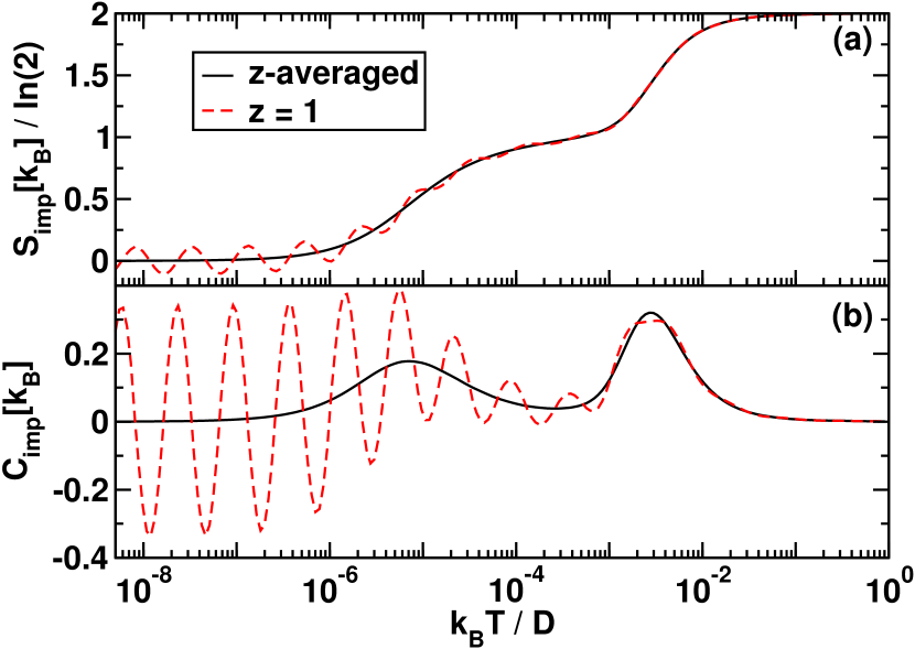
Figure 1: (Color online) Temperature dependence of, (a), the impurity entropy, $S_{\rm imp}(T)$, and, (b), the impurity specific heat, $C_{\rm imp}(T)$, for the symmetric Anderson model with $U/\Delta_{0}=12$ and $\Delta_{0}=0.001D$. The calculations are for $\Lambda=4$ with an energy cut-off $e_{c}(\Lambda=4)=40$, without $z$-averaging [$n_{z}=1$, $z=1$ (dashed lines)], and with $z$-averaging [$n_{z}=2$, $z=1/4,\,3/4$ (solid lines)]. For $\Lambda=4$ two $z$ values suffice to eliminate the discretization oscillations.

Unless otherwise specified, the NRG calculations presented in this paper will be for a band of half-width $D=1$ and a constant particle-hole symmetric density of states $N_{F}=1/2D$. The hybridization strength, $\Delta_{0}$, defined as the half-width of the resonant level is given by $\Delta_{0}=\pi N_{F}V^{2}$. Calculations for the positive and negative-$U$ Anderson models include a ${\rm U}(1)$ symmetry for total electron number conservation and ${\rm SU}(2)$ symmetry for total spin conservation. We use the discretization scheme of Campo and Oliveira in Ref. Campo and Oliveira, 2005.

Figure 1 shows the temperature dependence of the specific heat and entropy, calculated with the above procedure, for the symmetric Anderson model with $U/\Delta_{0}=12$ and $\Delta_{0}=0.001D$. The calculations are for $\Lambda=4$ using an energy cut-off $e_{c}(\Lambda=4)=40$, both without $z$-averaging ($n_{z}=1$) and with $z$-averaging ($n_{z}=2$). Note the aforementioned oscillations in the case of no $z$-averaging ($n_{z}=1$). For $\Lambda=4$, two $z$ values suffice to eliminate the discretization oscillations (whereas for $\Lambda=10$, four values are required). In order to quantify the accuracy of the NRG calculations, we also solved numerically the thermodynamic Bethe ansatz equations for the Anderson model and calculated the entropy and specific heat (see Appendix B for details). A comparison of the $z$-averaged NRG calculations with the exact Bethe ansatz results, shown in Fig. 2, indicates very good agreement. Nevertheless, in the next section we show that the specific heat can be calculated directly from the impurity contribution to the internal energy in terms of local static correlation functions and that discretization effects within this approach are less pronounced than those above.

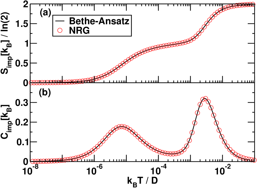
Figure 2: (Color online) Temperature dependence of, (a), the impurity entropy, $S_{\rm imp}(T)$, and, (b), the impurity specific heat, $C_{\rm imp}(T)$, for the symmetric Anderson model with $U/\Delta_{0}=12$ and $\Delta_{0}=0.001D$. Symbols: NRG calculations using the conventional approach. Solid lines: Bethe ansatz calculations. The NRG calculations are $z$-averaged with $n_{z}=2$ and other parameters as in Fig. 1.

III Impurity internal energy and specific heats

The impurity internal energy is defined by $E_{\rm imp}=E_{\rm total}-E_{0}$ where $E_{\rm total}=\langle H\rangle$ and $E_{0}=\langle H_{0}\rangle=\sum_{k\sigma}\epsilon_{k}\langle c_{k\sigma}^{\dagger}c_{k\sigma}\rangle_{\rm 0}$, where the subscript $0$ denotes a thermodynamic average for non-interacting conduction electrons (i.e., impurity is absent). We have

$$E_{0}=\sum_{\sigma}\int d\epsilon f(\epsilon)\epsilon N(\epsilon),$$ (7)

where $f(\epsilon)$ is the Fermi function and $N(\epsilon)=\sum_{k}\delta(\epsilon-\epsilon_{k})$ is the non-interacting conduction electron density of states per spin. $E_{\rm total}$ has four contributions:

$$E_{\rm total}=E_{\rm occ}+E_{\rm docc}+E_{\rm cond}+E_{\rm hyb},$$ (8)

where $E_{\rm occ}=\sum_{\sigma}\varepsilon_{d}\langle n_{d\sigma}\rangle$, $E_{\rm docc}=U\langle n_{d\uparrow}n_{d\downarrow}\rangle$, $E_{\rm cond}=\sum_{k\sigma}\epsilon_{k}\langle c_{k\sigma}^{\dagger}c_{k\sigma}\rangle$ and $E_{\rm hyb}=V\sum_{k\sigma}\langle c_{k\sigma}^{\dagger}d_{\sigma}+d^{\dagger}_{\sigma}c_{k\sigma}\rangle$. The first two contributions are evaluated as thermodynamic averages within the NRG calculation, requiring the calculation of matrix elements of $\sum_{\sigma}n_{d\sigma}$ and the double occupancy operator $\hat{D}_{\rm occ}=n_{d\uparrow}n_{d\downarrow}$. The contribution $E_{\rm hyb}$ may also be evaluated as a thermodynamic average $E_{\rm hyb}=V\sum_{\sigma}\langle d_{\sigma}^{\dagger}f_{0\sigma}+H.c.\rangle$. For the discussion below it is useful to note that the contribution $E_{\rm hyb}$ can also be expressed in terms of the local retarded d-electron Green function $G_{d\sigma}(\omega)=\langle\langle d_{\sigma};d_{\sigma}^{\dagger}\rangle\rangle_{\omega+i\delta}$ and the hybridization function $\Delta(\omega)=\sum_{k}V^{2}/(\omega+i\delta-\epsilon_{k})$ as

$$E_{\rm hyb}=-\frac{2}{\pi}\sum_{\sigma}\int d\omega f(\omega){\rm Im}\left[G_{d\sigma}(\omega)\Delta(\omega)\right].$$ (9)

Next, consider the contribution $E_{\rm cond}=\sum_{k\sigma}\epsilon_{k}\langle c_{k\sigma}^{\dagger}c_{k\sigma}\rangle$. This is not simply $E_{0}$ since the impurity affects the conduction electrons once $V$ is finite. It can be evaluated from the equation of motion of the retarded conduction electron Greens function $G_{k\sigma}(\omega)=\langle\langle c_{k\sigma};c_{k\sigma}^{\dagger}\rangle\rangle_{\omega+i\delta}$:

$$G_{k\sigma}=G_{k\sigma}^{0}+G_{k\sigma}^{0}{\cal T}_{\sigma}G_{k\sigma}^{0}.$$ (10)

Here, ${\cal T}_{\sigma}(\omega)=V^{2}G_{d\sigma}(\omega)$ is the local ${\rm T}$-matrix and $G_{k\sigma}^{0}(\omega)=1/(\omega+i\delta-\epsilon_{k})$ is the non-interacting conduction electron Greens function. Using

$$\langle c_{k\sigma}^{\dagger}c_{k\sigma}\rangle=-\frac{1}{\pi}\int d\omega f(\omega){\rm Im}\left[\langle\langle c_{k\sigma};c_{k\sigma}^{\dagger}\rangle\rangle\right]$$

we find for $E_{\rm cond}$

$$E_{\rm cond}=E_{0}+E_{\rm int},$$

where

$$E_{\rm int} = -\frac{1}{\pi}\sum_{\sigma}\int d\omega f(\omega)\int d\epsilon{\rm Im}\left[\frac{\epsilon V^{2}N(\epsilon)}{(\omega+i\delta-\epsilon)^{2}}G_{d\sigma}(\omega)\right]$$

$$= -\frac{1}{\pi}\sum_{\sigma}\int d\omega f(\omega){\rm Im}\left[G_{d\sigma}(\omega)I(\omega)\right]$$

where $I(\omega)$ is given by

$$I(\omega)=-\frac{1}{\pi}\int d\epsilon\frac{\epsilon\Delta_{\rm I}(\epsilon)}{(\omega+i\delta-\epsilon)^{2}}=-\frac{\partial}{\partial\omega}\left(\omega\Delta(\omega)\right)$$

with $\Delta_{\rm I}(\epsilon)={\rm Im}\left[\Delta(\epsilon+i\delta)\right]=-\pi V^{2}N(\epsilon)$, and we evaluated $I(\omega)$ analytically by noting that $\Delta(\omega+i\delta)$ has the same properties as a retarded Green function (see Appendix A for details). We therefore find,

$$E_{\rm int} = \frac{1}{\pi}\sum_{\sigma}\int d\omega f(\omega){\rm Im}\left[G_{d\sigma}(\omega)\frac{\partial}{\partial\omega}\left(\omega\Delta(\omega)\right)\right]$$ (11)

$$= E_{\rm int}^{(1)}+E_{\rm int}^{(2)},$$

$$E_{\rm int}^{(1)} = \frac{1}{\pi}\sum_{\sigma}\int d\omega f(\omega){\rm Im}\left[G_{d\sigma}(\omega)\Delta(\omega)\right]$$ (12)

$$E_{\rm int}^{(2)} = \frac{1}{\pi}\sum_{\sigma}\int d\omega f(\omega){\rm Im}\left[G_{d\sigma}(\omega)\omega\frac{\partial\Delta(\omega)}{\partial\omega}\right]$$ (13)

From this and Eq. (9) we see that $E_{\rm int}^{(1)}=-\frac{1}{2}E_{\rm hyb}$. Hence, the impurity contribution to the internal energy, $E_{\rm imp}=E_{\rm total}-E_{0}$, is given by

$$E_{\rm imp} = E_{\rm occ}+E_{\rm docc}+\frac{1}{2}E_{\rm hyb}+E_{\rm int}^{(2)},$$ (14)

$$= E_{\rm ionic}+\frac{1}{2}E_{\rm hyb}+E_{\rm int}^{(2)},$$ (15)

where $E_{\rm ionic}=\langle H_{\rm imp}\rangle=E_{\rm occ}+E_{\rm docc}$ is adiabatically connected to the energy of the impurity decoupled from the band (i.e., its energy at $V\rightarrow 0$). All contributions to $E_{\rm imp}$, except for the last one, can be evaluated as thermodynamic averages of local static correlation functions: The contribution $E_{\rm int}^{(1)}$ from the band which involves a finite frequency Greens function has been related to $E_{\rm hyb}$, which can be evaluated as local static correlation function $V\sum_{\sigma}\langle d^{\dagger}_{\sigma}f_{0\sigma}+H.c.\rangle$. The contribution $E_{\rm int}^{(2)}$, also involves a finite frequency Greens function, but we could not express this as a local static correlation function. Its temperature dependence, however, is negligible since the main temperature dependence arises from the Fermi window $|\omega|<T$, but this region is cut out in $E_{\rm int}^{(2)}$ due to the factor of $\omega$. In addition, for many cases of interest $\partial\left(\Delta(\omega)\right)/\partial\omega$ is small and vanishes in the wide band limit: $D\rightarrow\infty$ and $\Delta_{0}=\pi N(0)V^{2}$ fixed. For example, for a constant density of states it equals $\frac{2\Delta_{0}}{\pi D}(1-(\omega/D)^{2})^{-1}\sim\Delta_{0}/D$ for $\omega\ll D$. Thus, to a very good approximation, which we shall quantify in the rest of the paper with detailed numerical calculations and comparisons to exact Bethe ansatz results, we can approximate the impurity contribution to the specific heat and entropy via $\bar{E}_{\rm imp}=E_{\rm ionic}+\frac{1}{2}E_{\rm hyb}$ as

$$C_{\rm imp}(T) = \frac{\partial\bar{E}_{\rm imp}}{\partial T}=\frac{\partial E_{\rm occ}}{\partial T}+\frac{\partial E_{\rm docc}}{\partial T}+\frac{1}{2}\frac{\partial E_{\rm hyb}}{\partial T}$$ (16)

$$= \frac{\partial E_{\rm ionic}}{\partial T}+\frac{1}{2}\frac{\partial E_{\rm hyb}}{\partial T},$$

$$S_{\rm imp}(T) = \int_{0}^{T}dT^{\prime}\frac{C_{\rm imp}(T^{\prime})}{T^{\prime}}.$$ (17)

The omitted term, $\partial E_{\rm int}^{(2)}/\partial T$, in (16) as argued above, has a negligible temperature dependence (although its magnitude is not necessarily always small compared to the terms retained). Notice that $\bar{E}_{\rm imp}$ is made up of a term due to the partial occupation of the local resonant level ($E_{\rm occ}$), a term due to the Coulomb repulsion of electrons in this level ($E_{\rm docc}$), and, a term due to the energy gained by hybridization of the local level with the conduction electrons ($E_{\rm hyb}/2$), that is, it involves only local static correlation functions. Such quantities can be calculated very accurately and efficiently within the NRG method, within a single calculation for the total system only, a significant advantage of this approach. In some situations, the hybridization function $\Delta(\omega)$ may be strongly asymmetric and have a strong energy dependence close to $\omega=0$. In such cases, the term $E_{\rm int}^{(2)}$ can be calculated via the local spectral function and included in $E_{\rm imp}$, which is possible within the NRG, at somewhat higher numerical cost. Another advantage of the present approach, is that discretization oscillations are far smaller for local quantities appearing in $\bar{E}_{\rm imp}$ than for extensive quantities, such as $\langle H\rangle$ and $\langle(H-\langle H\rangle)^{2}\rangle$ appearing in the conventional approach to specific heats. Figure 3 shows the specific heat and entropy calculated with the above method, for the same parameters as in Fig. 1-2, with and without $z$-averaging. One sees that the discretization oscillations in the case of no $z$-averaging ($n_{z}=1$ curves) are drastically smaller than for the corresponding $n_{z}=1$ results from the conventional approach in Fig. 1. Including $z$-averaging makes the results of the new procedure indistinguishable from the Bethe ansatz calculations, as will be discussed in detail in Sec. IV-V.

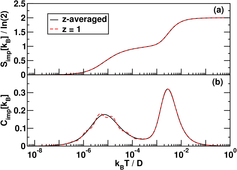
Figure 3: (Color online) Temperature dependence of, (a), the impurity entropy, $S_{\rm imp}(T)$, and, (b), the impurity specific heat, $C_{\rm imp}(T)$, for the symmetric Anderson model with $U/\Delta_{0}=12$ and $\Delta_{0}=0.001D$ calculated within NRG using the new approach for $\Lambda=4$ with an energy cut-off $e_{c}(\Lambda=4)=40$. Solid lines: $n_{z}=2$ ($z$-averaging). Dashed lines: $n_{z}=1$ (no $z$-averaging). For $\Lambda=4$ two $z$ values thus suffice to eliminate the discretization oscillations at $n_{z}=1$.

In Fig. 4(a), we show the different contributions $E_{\rm occ}$, $E_{\rm docc}$ and $E_{\rm hyb}/2$ to the impurity internal energy for the symmetric Anderson model. Their temperature derivatives $C_{\rm occ}$ , $C_{\rm docc}$ and $C_{\rm hyb}$ give the relative contributions of these terms to the impurity specific heat $C_{\rm imp}$ and are shown in Fig. 4(b). Notice, that the Kondo induced peak in $C_{\rm imp}$ at low temperatures results from a delicate balance of the hybridization ($C_{\rm hyb}$) and Coulomb contributions ($C_{\rm docc}$), while the peak due to the resonant level at high temperatures is mainly due to the Coulomb term. The latter trend persists also for the asymmetric model, as shown in Fig. 5. Notice also that the gain in energy due to hybridization diminishes at high temperatures, reflecting the decoupling of the impurity from the conduction electrons in this limit. In general, however, the interaction of the impurity with the environment via the hybridization term provides an essential contribution at all non-zero hybridization strengths.

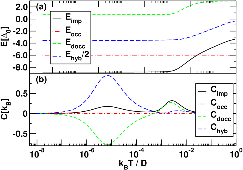
Figure 4: (Color online) (a) The individual contributions $E_{\rm occ}$, $E_{\rm docc}$, and $E_{\rm hyb}$ to $E_{\rm imp}$ as a function of temperature (in units of $\Delta_{0}$) for the symmetric model with parameters as in Fig. 1 ($z$-averaged with $n_{z}=2$). (b) Temperature derivatives of the above, yielding the relative contributions $C_{\rm occ}$, $C_{\rm docc}$, and $C_{\rm hyb}$ to the specific heat $C_{\rm imp}$.

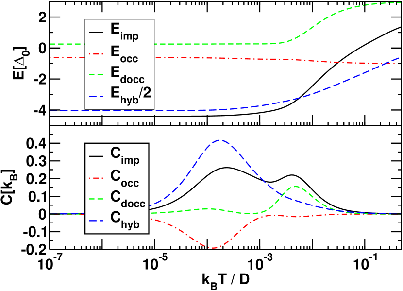
Figure 5: (Color online) (a) The individual contributions $E_{\rm occ}$, $E_{\rm docc}$, and $E_{\rm hyb}$ to $E_{\rm imp}$ as a function of temperature (in units of $\Delta_{0}$) for the asymmetric model with parameters as in Fig. 1, but for an asymmetric level position $\varepsilon_{d}/\Delta_{0}=-1$ ($z$-averaged with $n_{z}=2$). (b) Temperature derivatives of the above, yielding the relative contributions $C_{\rm occ}$, $C_{\rm docc}$, and $C_{\rm hyb}$ to the specific heat $C_{\rm imp}$.

We now quantify the error in neglecting $\partial E_{\rm int}^{(2)}(T)/\partial T$ in Eq. (16) for the calculation of impurity specific heats by, (a), comparing the result for $C_{\rm imp}$ obtained within the new method with the Bethe ansatz calculations, and, (b), explicitly calculating the contribution $\partial E_{\rm int}^{(2)}(T)/\partial T$. Figure 6(a) shows the comparison to the Bethe ansatz calculation, where we also include the specific heat from the conventional approach. The relative deviation of the NRG calculations to the Bethe ansatz, shown in Fig. 6(b), is below $1\%$ for all temperatures $T<0.01=10\Delta_{0}$. For $T\ll T_{\rm K}$, the relative error in $C_{\rm imp}$ from the internal energy is $0.1\%$ and $0.5\%$ in the conventional approach. The relative error exhibits remnants of the discretization oscillations, which are not completely eliminated with $z$-averaging. Notice also that the errors in the two NRG calculations have the same error (relative to the Bethe ansatz) in the high temperature limit, $T\gg\Delta_{0}$. Hence, the latter error is not due to neglect of $E_{\rm int}^{(2)}$ in Eq. (15). Instead, it reflects, (a), the different high energy cut-off schemes in NRG and Bethe ansatz, and, (b), the finite size errors in the high energy excitation spectrum in NRG, since the latter stem from the shortest chains diagonalized (typically $m=4-6$), which are also the ones most sensitive to the logarithmic discretization. The fact that the errors in both NRG calculations also correlate at lower temperatures ($T\lesssim\Delta_{0}$) suggests that the neglect of $E_{\rm int}^{(2)}$ in Eq. (15) is not the main source of error in calculating $C_{\rm imp}(T)$. An explicit calculation that illustrates this is shown in Fig. 7. As stated above, the value of $E_{\rm int}^{(2)}$ is of order $\Delta_{0}/\pi$, however, one clearly sees in Fig. 7(a) that $E_{\rm int}^{(2)}$ has little temperature dependence (relative to the other contributions) for all temperatures extending up to the bandwidth $D=1$. It’s relative contribution to the impurity specific heat, shown in Fig. 7(b), for an energy dependent $\Delta(\omega)$, is negligible, typically contributing below $0.5\%$.

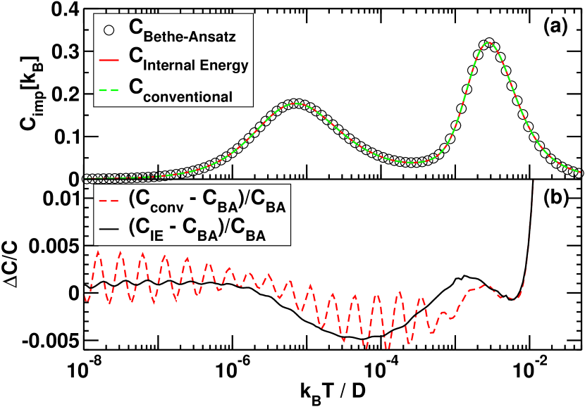
Figure 6: (Color online) (a) Comparison of specific heat, $C_{\rm imp}(T)$, from the impurity internal energy (solid line) and conventional approach (dashed line) with the Bethe ansatz calculation (symbols) for the symmetric Anderson model with parameters as in Fig. 1. NRG parameters also as in Fig. 1 with $n_{z}=2$. (b) The relative deviation with respect to the Bethe ansatz result of the new (solid line) and conventional (dashed line) approaches.

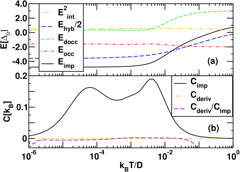
Figure 7: (Color online) (a) The contribution $E_{\rm int}^{(2)}$ to $E_{\rm imp}$ as a function of temperature compared with $E_{\rm occ}$, $E_{\rm docc}$ and $E_{\rm hyb}$ (in units of $\Delta_{0}$) for the asymmetric model. Model parameters: $U=12\Delta_{0}$, $\Delta_{0}=0.001D$, $\varepsilon_{d}/\Delta_{0}=-2$ with a semi-elliptic hybridization function ${\rm Im}[\Delta(\omega)]=-\frac{\Delta_{0}}{D}\sqrt{(D^{2}-\omega^{2})}$. A small $\Lambda=1.5$ was used, which allows the spectral function entering $E_{\rm int}^{(2)}$ to be obtained without $z$-averaging. (b) The contribution $C_{\rm deriv}=\partial E_{\rm int}^{(2)}(T)/\partial T$ to $C_{\rm imp}$. The relative size of $C_{\rm deriv}$ to $C_{\rm imp}$ lies between $0.2\%$ and $0.5\%$ for all temperatures, except at temperatures approaching the bandwidth $D=1$.

IV Results for the symmetric model

In this section we show results for the entropy and specific heat of the Anderson model at the particle-hole symmetric point $\varepsilon_{d}=-U/2$. Results for zero magnetic field and increasing correlation strength $U/\Delta_{0}$ are presented in Sec. (IV.1) and results for finite magnetic fields are given in Sec. (IV.2).

The symmetric Anderson model has been investigated in detail Hewson (1997) and is well understood. For $U/\Delta_{0}\gg 1$ and $-\varepsilon_{d}\gg\Delta_{0}$, a local spin $S=1/2$ magnetic moment forms on the impurity. In this limit, the physics of the symmetric model at low temperatures $T\ll{\rm min}(|\varepsilon_{d}+U|,|\varepsilon_{d}|,D)$ is that of the Kondo model

$$H_{\rm K}=H_{0}+J{\bf S}.{\bf s}_{0},$$ (18)

where, $J$ is an antiferromagnetic exchange coupling between the local spin $S$ and the conduction electron spin-density ${\bf s}_{0}$ at the impurity site. The value of $J$ is given by the Schrieffer-Wolff transformationSchrieffer and Wolff (1966) $J=4V^{2}/U$. The low temperature properties (for $U\gg\Delta_{0}$) are universal functions of $T/T_{\rm K}$ and $B/T_{\rm K}$ where we choose to define the Kondo scale from the Bethe ansatz result for the $T=0$ susceptibility $\chi(0)$ via $\chi(0)=(g\mu_{\rm B})^{2}/4T_{\rm K}$. For $U\gg\Delta_{0}$, $T_{\rm K}$ is given by

$$T_{\rm K}=\sqrt{U\Delta_{0}/2}e^{-\pi U/8\Delta_{0}+\pi\Delta_{0}/2U},$$ (19)

within corrections which are exponentially small in $U/\pi\Delta_{0}$ (see Ref. Hewson, 1997). For $U=0$, the symmetric Anderson model reduces to a resonant level model and the relevant low temperature scale is then $\Delta_{0}$.

IV.1 Zero magnetic field

A comparison of the new approach with Bethe ansatz calculations is shown in Fig. 8 for the temperature dependence of the impurity specific heat and entropy for increasing values of the Coulomb interaction $U/\Delta_{0}$. For $U/\Delta_{0}=12$, the Kondo induced peak in the specific heat at $T_{\rm p}=\alpha T_{\rm K}$ with $\alpha\approx 0.29$ is well separated from the peak at $T\approx|\varepsilon_{d}|$ due to the resonant level. With decreasing $U/\Delta_{0}$, the Kondo effect is suppressed and the Kondo induced peak in $C(T)$ eventually merges with the peak due to the resonant level for $U/\Delta_{0}\rightarrow 0$. Good agreement between the NRG and the exact Bethe ansatz calculations is seen for all values of $U/\Delta_{0}$.

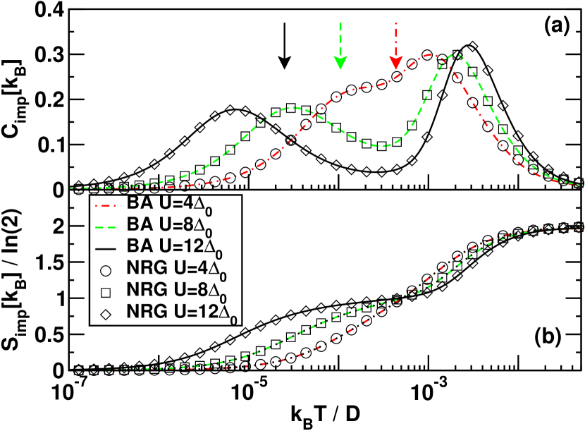
Figure 8: (Color online) Temperature dependence of, (a), the impurity specific heat, $C_{\rm imp}(T)$, and, (b), the impurity entropy, $S_{\rm imp}(T)/\ln(2)$, for the symmetric Anderson model with $\Delta_{0}=0.001D$ and increasing values of the Coulomb interaction: $U/\Delta_{0}=4,8,12$. Arrows in (a) indicated the Kondo scale $T_{\rm K}$ defined in Eq. 19. Symbols: new approach using NRG with $\Lambda=4$ with an energy cut-off $e_{c}(\Lambda=4)=40$, and $z$-averaging [$n_{z}=2$, $z=1/4,\,3/4$]. Lines: corresponding Bethe ansatz calculations.

IV.2 Finite magnetic field

At finite magnetic fields $B>0$, the ${\rm SU}(2)$ spin symmetry which we use in the NRG calculations, is broken. Therefore, in order to carry out calculations at finite magnetic field $B>0$, preserving the numerical advantages of the full ${\rm SU}(2)$ symmetry, such as the increased number of states that can be retained, we obtained the finite field results by mapping the symmetric positive $U$ Anderson model onto the negative-$U$ Anderson model in the absence of a magnetic field but with local level given by $\varepsilon_{d}=-U/2-B/2$ with $U$ negative. Iche and Zawadowski (1972); Hewson et al. (2006) This correspondence results from a particle-hole transformation on the down spins only: $d{{}_{\downarrow}}\rightarrow d_{\downarrow}^{\dagger},\,d{{}_{\uparrow}}\rightarrow d_{\uparrow}$, and $c_{k\downarrow}\rightarrow c_{-k\downarrow}^{\dagger},c_{k\uparrow}\rightarrow c_{k\uparrow}$ with a particle-hole symmetric band $\epsilon_{k}=-\epsilon_{-k}$.

Figure 9 shows the temperature dependence of $C_{\rm imp}(T,B)$ for $B/T_{\rm K}\geq 1$ using our new approach and compared with Bethe ansatz calculations. The Kondo peak in the specific heat shifts to higher fields with increasing $B$ and its position scales as $B^{2}/T_{\rm K}$ for $T_{\rm K}\ll B\ll\varepsilon_{d}$. In contrast, the resonant level peak remains approximately fixed at $T\approx\varepsilon_{d}$. As $B$ approaches the value $\varepsilon_{d}$, the two peaks merge into one peak at $T\approx\varepsilon_{d}$, with aproximately twice the height of the $B=0$ resonant level peak, and containing the whole entropy $S_{\rm imp}/k_{\rm B}=\ln(4)$. The low field behaviour of $C_{\rm imp}(T,B)$, also compared to Bethe ansatz calculations, is shown in Fig. 9(a) as $T_{\rm K}\gamma(T,B)=C_{\rm imp}(T,B)/(T/T_{\rm K})$ versus $T/T_{\rm K}$ for $B/T_{\rm K}\leq 2$. For $T,B\rightarrow 0$, $\gamma(T,B)\rightarrow\gamma(0,0)\sim 1/T_{\rm K}$ where $\gamma(0,0)$ is the linear coefficient of specific heat. This is strongly enhanced for $U/\Delta_{0}\gg 1$ due to the exponential decrease of $T_{\rm K}$. A finite magnetic field of order $T_{\rm K}$ significantly suppresses the Kondo effect and results in smaller values of $\gamma(0,B)$. As another check on the accuracy of our calculations, we estimate the Wilson ratio $R_{\rm W}=4\pi^{2}\chi(0)/3\gamma(0,0)$. This takes the value $2$ in the Kondo regime of the symmetric Kondo model (i.e., for $U\gg\Delta_{0}$) From the definition of $T_{\rm K}$, we have that the susceptibility $\chi(0)=1/4T_{\rm K}$, and from Fig. 9(a) we extract $\gamma(0,0)\approx 1.64/T_{\rm K}$, resulting in $R_{\rm W}\approx 2.006$, that is, a relative error in $R_{\rm W}$ below $1\%$.

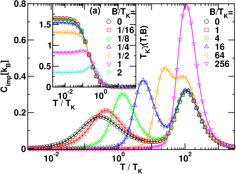
Figure 9: (Color online) Temperature dependence of the impurity specific heat, $C_{\rm imp}(T,B)$, for the symmetric Anderson model for $U/\Delta_{0}=12$, $\Delta_{0}=0.001D$ and increasing values of the magnetic field $B/T_{\rm K}\geq 1$ where the Kondo scale $T$ is defined in Eq. 19. Symbols: NRG calculations $\Lambda=4$ with an energy cut-off $e_{c}(\Lambda=4)=40$, and $z$-averaging [$n_{z}=2$, $z=1/4,\,3/4$]. Lines: Bethe ansatz calculations. Inset (a): $T_{\rm K}\gamma(T,B)$ versus $T/T_{\rm K}$ for several values of $B/T_{\rm K}\leq 2$, where $\gamma(T,B)=C_{\rm imp}(T,B)/T$.

V Results for the asymmetric model

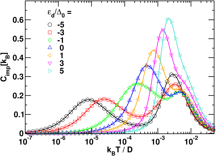
Figure 10: (Color online) Temperature dependence of $C_{\rm imp}(T)$ for $U/\Delta_{0}=12,\,\Delta_{0}=0.001D$ and local level positions $\varepsilon_{d}/\Delta_{0}$ ranging from Kondo ($\varepsilon_{d}/\Delta_{0}\leq-1$), mixed valence ($|\varepsilon_{d}/\Delta_{0}|\leq 1$), and empty orbital ($\varepsilon_{d}/\Delta_{0}>1$) regimes. Symbols: NRG calculations (new approach, $z$-averaging and NRG parameters as in Fig. 1). Lines: Bethe ansatz calculations.

Figure 10 shows the impurity specific heat versus temperature for the asymmetric Anderson model, that is, for $\varepsilon_{d}>-U/2$, calculated within the new approach. For comparison, we also show the corresponding Bethe ansatz calculations. One sees again excellent agreement at all temperatures between the two methods. Results for $\varepsilon_{d}<-U/2$ are not shown, since these can be obtained from results for $\varepsilon_{d}>-U/2$ by noting that the Anderson model with parameters $\varepsilon_{d},U,V$ transforms, under a particle-hole transformation applied to both spin species, to an Anderson model with parameters $-(\varepsilon_{d}+U),U,V$. This holds for a particle-hole symmetric constant density of states, the case considered here.

The specific heat curves for the asymmetric model are more complicated than those of the symmetric model. In the latter, the relevant excitations were the low temperature spin flip excitations, characterized by the Kondo scale $T_{\rm K}$, and the excitations involving addition or removal of an electron from the resonant level, both characterized by an energy $|\varepsilon_{d}|=U/2$. This accounts for the two peaks in the specific heat of the symmetric model: A high temperature peak at $T\approx|\varepsilon_{d}|$ and a low temperature Kondo induced peak at $T\approx T_{\rm K}$. For the asymmetric Anderson model, three types of excitation are possible: Low-temperature spin flip excitations, associated with the Kondo scale $T_{\rm L}=\sqrt{U\Delta_{0}/2}e^{-\pi|\varepsilon_{d}|\,|\varepsilon_{d}+U|/2U\Delta_{0}}$ of the asymmetric model,Hewson (1997) and excitations associated with, (i), removing an electron from a singly occupied level (with energy scale $|\varepsilon_{d}|$) and (ii), removing an electron from a doubly occupied level (with energy scale $|\varepsilon_{d}+U|$). Thus, three peaks can be present in $C_{\rm imp}(T)$: a Kondo induced peak at $T\approx T_{\rm L}$, and two charge fluctuation induced peaks at $T\approx T_{1}=|\varepsilon_{d}|$ and $T\approx T_{2}=|\varepsilon_{d}+U|$, respectively. In Fig. 10, the two high temperature peaks are seen in the mixed valence regime and partly also in the empty orbital regime (where the upper peak at $T_{2}$ appears as a shoulder of the main peak at $T_{1}$). However, in the Kondo regime, the cases $\varepsilon_{d}/\Delta_{0}=-5,-3$ with the choice $U=12\Delta_{0}$ result in $T_{1}/\Delta_{0}=5,3$ and $T_{2}/\Delta_{0}=7,9$. In these cases, $T_{1}$ and $T_{2}$ are too close for separate peaks to be seen. In order to clarify this, we carried out calculations for $U=48\Delta_{0}\gg\Delta_{0}$, and $\varepsilon_{d}/\Delta_{0}=-10,-8,-6,-4,-2$ in the Kondo regime, for which $T_{1}/\Delta_{0}=10,8,6,4,2$ and $T_{2}/\Delta_{0}=38,40,42,44,46\gg T_{1}/\Delta_{0}$ are disparate scales. Figure 11 shows how the peaks at $T\approx T_{1}$ and $T\approx T_{2}$ evolve from the peak at $T\approx|\varepsilon_{d}|=U/2$ of the symmetric model (dashed line in Fig. 11) on increasing $\varepsilon_{d}$ above $-U/2$. Simultaneously, the Kondo peak in the specific heat at $T_{\rm L}$ shifts to higher temperatures and eventually merges with the peak at $T_{1}$ when the mixed valence regime is reached (i.e., for $\varepsilon_{d}=-\Delta_{0}$). Thereafter, only the high temperature peaks at $T_{1}$ and $T_{2}$ are present. Notice also, that in the mixed valence regime $T_{1}$ differs significantly from $|\varepsilon_{d}|$, a result of non-trivial renormalizations present in the mixed valence regime, but absent in the empty orbital regime.

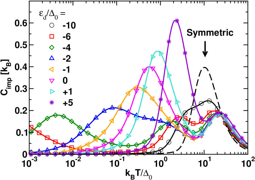
Figure 11: (Color online) Temperature dependence of $C_{\rm imp}(T)$ for $U/\Delta_{0}=48,\,\Delta_{0}=0.0001D$ and local level positions $\varepsilon_{d}/\Delta_{0}=-10,-6,-4,-2$ (Kondo regime), $\varepsilon_{d}/\Delta_{0}=-1,0,+1$ (mixed valence regime) and $\varepsilon_{d}/\Delta_{0}=+5$ (empty orbital regime). NRG using the new approach (symbols) and conventional approach (solid lines) [$\Lambda=20,n_{z}=4,e_{c}(\Lambda)=130$]. Dashed line: resonant level peak in $C_{\rm imp}$ at $T/\Delta_{0}\approx|\varepsilon_{d}|/\Delta_{0}=U/2\Delta_{0}=24$ for the symmetric model (the Kondo induced peak at much lower $T$ is not shown). The two high temperature peaks of the asymmetric model evolve from this peak when the asymmetry is finite.

VI Generalization to other models

The approach of Sec. III can be straightforwardly generalized to multiorbital and multichannel Anderson impurity models with arbitrary local Coulomb interactions, as we briefly outline in Sec. VI.1. In addition, in Sec. VI.2 we discuss it’s application to dissipative two state systems and the anisotropic Kondo model (AKM).

VI.1 Multiorbital and multichannel Anderson models

The multiorbital and multichannel Anderson impurity model is given by $H=H_{\rm imp}+H_{\rm 0}+H_{\rm int}$, where $H_{\rm imp}=\sum_{\alpha\sigma}\varepsilon_{\alpha}d_{\alpha\sigma}^{\dagger}d_{\alpha\sigma}+H_{\rm C}(U,U^{\prime},J)$, describes the impurity with a set of local levels having energies $\varepsilon_{d\alpha},\alpha=1,\dots,g$ and $H_{\rm C}(U,U^{\prime},J)$ is the local Coulomb interaction involving intra-orbital $U$, inter-orbital $U^{\prime}$ and a Hund’s exchange term $J$. The conduction electrons are described by $H_{\rm 0}=\sum_{k\alpha\sigma}\epsilon_{k\alpha}c_{k\alpha\sigma}^{\dagger}c_{k\alpha\sigma}$ where $\epsilon_{k\alpha}$ is the kinetic energy of electrons in band $\alpha$. These bands hybridize with hybridization strengths $V_{\alpha},\alpha=1,\dots,g$ to the local levels via $H_{\rm int}=\sum_{k\alpha\sigma}V_{\alpha}(c_{k\alpha\sigma}^{\dagger}d_{\alpha\sigma}+d^{\dagger}_{\alpha\sigma}c_{k\alpha\sigma})$. Let $\Delta_{\alpha}(\omega)=\sum_{k}V_{\alpha}^{2}/(\omega-\epsilon_{k\alpha})$ denote the hybridization functions characterizing $H_{\rm int}$. Proceeding as in Sec. III, we write the impurity internal energy as $E_{\rm imp}=E_{\rm total}-E_{\rm 0}$ where $E_{\rm total}=\langle H\rangle$ is the total energy and $E_{\rm 0}=\langle H_{0}\rangle=\sum_{k\alpha\sigma}\epsilon_{k\alpha}\langle c_{k\alpha\sigma}^{\dagger}c_{k\alpha\sigma}\rangle_{\rm 0}$ is the energy of the non-interacting conduction electrons in the absence of the impurity. The latter is given by $E_{0}=\sum_{\alpha\sigma}\int d\epsilon f(\epsilon)\epsilon N_{\alpha}(\epsilon),$ where $f(\epsilon)$ is the Fermi function and $N_{\alpha}(\epsilon)=\sum_{k}\delta(\epsilon-\epsilon_{k\alpha})$ is the non-interacting conduction electron density of states per spin for band $\alpha$. $E_{\rm total}$ is a sum of local occupation number contributions $E_{\rm occ}=\sum_{\alpha\sigma}\varepsilon_{\alpha}\langle n_{\alpha\sigma}\rangle$ and local Coulomb terms $E_{C}=\langle H_{\rm C}(U,U^{\prime},J)\rangle$ and two further terms involving the interacting band $E_{\rm cond}=\sum_{k\alpha\sigma}\epsilon_{k\alpha}\langle c_{k\alpha\sigma}^{\dagger}c_{k\alpha\sigma}\rangle$ and the hybridization energy $E_{\rm hyb}=\sum_{\alpha\sigma}V_{\alpha}\langle d_{\alpha\sigma}^{\dagger}f_{0\alpha\sigma}+H.c.\rangle$ where $V_{\alpha}f_{0\alpha\sigma}=\sum_{k}c_{k\alpha\sigma}$:

$$E_{\rm total}=E_{\rm occ}+E_{\rm C}+E_{\rm cond}+E_{\rm hyb}.$$ (20)

We evaluate the latter two contributions as in Sec. III, finding

$$E_{\rm hyb}=-\frac{2}{\pi}\sum_{\alpha\sigma}\int d\omega f(\omega){\rm Im}\left[G_{d\alpha\sigma}(\omega)\Delta_{\alpha}(\omega)\right],$$ (21)

and $E_{\rm cond}=E_{\rm 0}+E_{\rm int}$, where

$$E_{\rm int} = \frac{1}{\pi}\sum_{\alpha\sigma}\int d\omega f(\omega){\rm Im}\left[G_{d\alpha\sigma}(\omega)\frac{\partial}{\partial\omega}\left(\omega\Delta_{\alpha}(\omega)\right)\right]$$ (22)

$$= E_{\rm int}^{(1)}+E_{\rm int}^{(2)},$$

$$E_{\rm int}^{(1)} = \frac{1}{\pi}\sum_{\alpha\sigma}\int d\omega f(\omega){\rm Im}\left[G_{d\alpha\sigma}(\omega)\Delta_{\alpha}(\omega)\right]$$ (23)

$$E_{\rm int}^{(2)} = \frac{1}{\pi}\sum_{\alpha\sigma}\int d\omega f(\omega){\rm Im}\left[G_{d\alpha\sigma}(\omega)\omega\frac{\partial\Delta_{\alpha}(\omega)}{\partial\omega}\right],$$ (24)

and $G_{d\alpha\sigma}(\omega)$ is the retarded Green function for local level $\alpha$. Combining $E_{\rm int}^{(1)}$ with $E_{\rm hyb}$ gives for the impurity internal energy

$$E_{\rm imp}=E_{\rm occ}+E_{\rm C}+\frac{1}{2}E_{\rm hyb}+E_{\rm int}^{(2)},$$ (25)

where, as before, all contributions except the last one are evaluated as local static correlation functions. For reasons discussed in Sec. III, the temperature dependence of the last term is negligible in many cases and the impurity specific heat can be calculated to high accuracy via

$$C_{\rm imp} = \frac{\partial E_{\rm occ}}{\partial T}+\frac{\partial E_{\rm C}}{\partial T}+\frac{1}{2}\frac{\partial E_{\rm hyb}}{\partial T}$$ (26)

$$= \frac{\partial E_{\rm ionic}}{\partial T}+\frac{1}{2}\frac{\partial E_{\rm hyb}}{\partial T},$$ (27)

where $E_{\rm ionic}=\langle H_{\rm imp}\rangle$.

VI.2 Dissipative two state systems and the anisotropic Kondo model

The method of Sec. III can be applied to bosonic models such as the dissipative two state system,Leggett et al. (1987); Weiss (2008) and for Ohmic dissipation, one can further relate the results to the AKM and related models (for example, a two-level system in a metallic environment Ramos et al. (2003)). Dissipative two state systems are of interest in many contexts, including the description of qubits coupled to their environment.

The Hamiltonian of the dissipative two state system is given by $H=H_{\rm S}+H_{\rm B}+H_{\rm I}$. The first term $H_{\rm S}=-\frac{1}{2}\Delta_{0}\sigma_{x}+\frac{1}{2}\epsilon\sigma_{z}$ describes a two-level system with bias splitting $\epsilon$ and tunneling amplitude $\Delta_{0}$, and $\sigma_{i=x,y,z}$ are Pauli spin matrices. $H_{\rm B}=\sum_{i}\omega_{i}(a^{\dagger}_{i}a_{i}+1/2)$ is the environment and consists of an infinite set of harmonic oscillators ($i=1,2,\dots,\infty$) with $a_{i}(a_{i}^{\dagger})$ the annihilation (creation) operators for a harmonic oscillator of frequency $\omega_{i}$ and $0\leq\omega_{i}\leq\omega_{\rm c}$, where $\omega_{\rm c}$ is an upper cut-off frequency. The non-interacting density of states of the environment is denoted by $g(\omega_{i})=\sum_{i}\delta(\omega-\omega_{i})$ and is finite in the interval $[0,\omega_{\rm c}]$ and zero otherwise. Finally, $H_{\rm I}=\frac{1}{2}\sigma_{z}\sum_{i}\lambda_{i}(a_{i}+a_{i}^{\dagger})$ describes the coupling of the two-state system co-ordinate $\sigma_{z}$ to the oscillators, with $\lambda_{i}$ denoting the coupling strength to oscillator $i$. The function $\Gamma(\omega+i\delta)=\sum_{i}(\lambda_{i}/2)^{2}/(\omega-\omega_{i}+i\delta)=\int d\omega^{\prime}(\lambda(\omega^{\prime})/2)^{2}\,g(\omega^{\prime})/(\omega-\omega^{\prime}+i\delta)$ characterizes the system-environment interaction. The Ohmic two state system, specified by a spectral function $J(\omega)=-\frac{1}{\pi}{\rm Im}\Gamma(\omega+i\delta)\sim\alpha\omega$ for $\omega\rightarrow 0$, where $\alpha$ is the dimensionless dissipation strength, is equivalent to the AKM $H=\sum_{k\sigma}\epsilon_{k}c_{k\sigma}^{\dagger}c_{k\sigma}+\frac{J_{\perp}}{2}(S^{+}s_{\rm 0}^{-}+S^{-}s_{\rm 0}^{+})+J_{\parallel}S_{z}s_{0}^{z}+BS_{z}$, where $J_{\perp}$ ($J_{\parallel}$ is the transverse (longitudinal) part of the Kondo exchange interaction and $B$ is a local magnetic field. The correspondence is given by $\rho J_{\perp}=-\Delta_{0}/\omega_{\rm c}$ and $\alpha=(1+2\delta/\pi)^{2}$ where $\delta=\arctan(-\pi\rho J_{\parallel}/4)$ and $\rho$ is the density of states of the conduction electrons in the AKM. Guinea et al. (1985); Costi and Kieffer (1996); Leggett et al. (1987); Costi and Zarand (1999); Weiss (2008) The low energy scale of the Ohmic two state system is the renormalized tunneling amplitude $\Delta_{\rm r}$ given by $\Delta_{\rm r}/\omega_{\rm c}=(\Delta_{\rm 0}/\omega_{\rm c})^{1/(1-\alpha)}$ and corresponds to the low energy Kondo scale $T_{\rm K}$ of the AKM. Special care is needed to obtain results for the Ohmic two state system from the AKM in the vicinity of the singular point $\alpha\rightarrow 1^{-}$, since this corresponds to $J_{\parallel}\rightarrow 0$ but with the condition $0<J_{\perp}<J_{\parallel}$, that is, in terms of parameters of the Ohmic two state system one requires $\Delta_{\rm 0}/\omega_{\rm c}\ll 1-\alpha\ll 1$ in order to investigate the vicinity of $\alpha=1$ within the AKM.Weiss (2008)

The specific heat, $C_{\rm imp}=\partial E_{\rm imp}/\partial T$, of the Ohmic two-state system is defined via an impurity internal energy $E_{\rm imp}=E_{\rm total}-E_{\rm 0}$, where $E_{\rm total}=\langle H\rangle=\langle H_{\rm S}\rangle+\langle H_{\rm B}\rangle+\langle H_{\rm I}\rangle$ and $E_{\rm 0}=\langle H_{\rm B}\rangle_{\rm 0}=\sum_{i}\omega_{i}\langle a^{\dagger}_{i}a_{i}\rangle_{\rm 0}+E_{\rm zp}=\int_{0}^{\omega_{c}}d\omega\,\omega\,n(\omega)\,g(\omega)+E_{\rm zp}$ where $n(\omega)=1/(e^{\beta\omega}-1)$ is the Bose distribution function and the zero point energy $E_{\rm zp}$ can be dropped, as it cancels in the difference $\langle H_{\rm B}\rangle-E_{\rm 0}=E_{\rm B}-E_{\rm 0}$ appearing in $E_{\rm imp}$. Evaluating $E_{\rm B}-E_{\rm 0}$ and $E_{\rm I}=\langle H_{\rm I}\rangle$ following the approach in Sec. III, we find

$$E_{\rm B}-E_{\rm 0} = \frac{1}{\pi}\int d\omega n(\omega){\rm Im}\left[\chi_{zz}(\omega+i\delta)\frac{\partial}{\partial\omega}\left(\omega\Gamma(\omega+i\delta)\right)\right]$$ (28)

$$= E_{\rm B}^{(1)}+E_{\rm B}^{(2)},$$

$$E_{\rm B}^{(1)} = \frac{1}{\pi}\int d\omega n(\omega){\rm Im}\left[\chi_{zz}(\omega+i\delta)\Gamma(\omega+i\delta)\right]$$ (29)

$$E_{\rm B}^{(2)} = \frac{1}{\pi}\int d\omega n(\omega){\rm Im}\left[\chi_{zz}(\omega+i\delta)\omega\frac{\partial\Gamma(\omega+i\delta)}{\partial\omega}\right],$$ (30)

and

$$E_{\rm I} = -\frac{1}{\pi}\int d\omega n(\omega){\rm Im}\left[\chi_{zz}(\omega+i\delta)\Gamma(\omega+i\delta)\right],$$ (31)

where $\chi_{zz}(\omega+i\delta)=\langle\langle\sigma_{z};\sigma_{z}\rangle\rangle_{\omega+i\delta}$ is the longitudinal retarded dynamic susceptibility and $\Gamma(\omega+i\delta)$, characterizing the system-environment interaction, was defined above. Noting that $E_{\rm B}^{(1)}$ exactly cancels $E_{\rm I}$ in the impurity internal energy, we find

$$E_{\rm imp}=-\frac{1}{2}\Delta_{0}\langle\sigma_{x}\rangle+\frac{1}{2}\epsilon\langle\sigma_{z}\rangle+E_{\rm B}^{(2)},$$ (33)

that is, $E_{\rm imp}=E_{\rm S}+E_{\rm B}^{(2)}$. The term $E_{\rm B}^{(2)}$ gives a non-negligible contribution to the impurity internal energy. For example, in the Ohmic case with spectral function $J(\omega)=-\frac{1}{\pi}{\rm Im}\Gamma(\omega+i\delta)\sim\alpha\omega$ we have $\omega\partial J(\omega)/\partial\omega~{}\sim\alpha\omega$ at low frequencies, so $E_{\rm B}^{(2)}$ provides a contribution proportional to $\alpha$. By carrying out specific heat calculations on the AKM, we find numerically that the impurity specific heat is consistent with setting $E_{\rm B}^{(2)}=\frac{1}{2}\alpha\Delta_{0}\langle\sigma_{x}\rangle+A$, with $A$ being a weakly temperature dependent term, and negligible for calculating the specific heat, except in the limit $\alpha\rightarrow 1^{-}$. The latter limit is difficult to treat numerically because of the vanishing low energy scale $\Delta_{\rm r}$ for $\alpha\rightarrow 1^{-}$ (e.g., for $\Delta_{\rm 0}/\omega_{\rm c}=0.01$ and $\alpha=0.9$ we have $\Delta_{\rm r}/\omega_{\rm c}=10^{-20}$). Hence, except in this extreme limit, and as we show below by comparing with exact results, the impurity specific heat can be obtained accurately from $C_{\rm imp}=\frac{\partial E_{\rm imp}}{\partial T}$ by using

$$E_{\rm imp}\approx-\frac{1}{2}\Delta_{0}(1-\alpha)\langle\sigma_{x}\rangle+\frac{1}{2}\epsilon\langle\sigma_{z}\rangle.$$ (34)

Figure 12 shows results obtained in this way for $C_{\rm imp}(T)/({k_{\rm B}T/\Delta_{\rm r}})$ compared to Bethe ansatz calculations for the AKMCosti (1998) for a range of dissipation strengths. These results recover the known results for asymptotically high and low temperatures.Görlich and Weiss (1988) In common with specific heats of other correlated electron systems as a function of interaction strength,Chandra et al. (1999) we observe a crossing point in $C(T)/T$ (here, at $k_{\rm B}T/\Delta_{\rm r}\approx 0.67$). On decreasing the dissipation strength from strong ($\alpha>1/2$) to weak values ($\alpha<1/2$) the $T^{3}$ coefficient of the specific heat changes sign for $\alpha<1/3$ resulting in the appearance of a finite temperature peak in $C(T)/T$. This is shown in more detail in Fig. 13. It signifies the development of a gap $~{}\sim\Delta_{0}$ in the spectrum as $\alpha\rightarrow 0$. For $\alpha=0$ one eventually recovers the Schottky specific heat for a non-interacting two level system. The expression (34) for the Ohmic two system is also the impurity internal energy of the equivalent AKM (indeed, the NRG results that we showed were for this model). The correspondence of model parameters was given above and the operators $\sigma_{x}$ and $\sigma_{z}$ are identified, under bosonization,Guinea et al. (1985); Leggett et al. (1987); Weiss (2008); Costi and Zarand (1999) with the spin-flip operator $S^{+}s_{\rm 0}^{-}+S^{-}s_{\rm 0}^{+}$ and the local $S_{z}$ in the AKM, respectively. The zero temperature expectation values $\langle\sigma_{x}\rangle$ and $\langle\sigma_{z}\rangle$ (and the associated entanglement entropy of the qubit) have been studied previously as a function of dissipation strength and finite bias.Costi and McKenzie (2003); Hur (2008)

We expect that the term $E_{\rm B}^{(2)}$ is non-negligible also for generic spectral functions $J(\omega)\sim\omega^{s}$ and certainly for the sub-Ohmic case $s<1$. Recent results for the local spin dynamics of the sub-Ohmic spin boson model Florens et al. (2011) could shed light on this.

The result (34) shows that a significant contribution to the impurity internal energy and specific heat arises from the (interacting) bath contribution $E_{\rm B}^{(2)}$, which remains finite for arbitrarily small $\alpha$. Thus, while a definition of the internal energy of the system via $E_{\rm S}=\langle H_{\rm S}\rangle$ and the specific heat via $C_{\rm S}=\partial E_{\rm S}/\partial T$, might seem reasonable for a small quantum system weakly coupled to an infinite bath, such a definition yields, in general, a specific heat $C_{\rm S}$ which differs from $C_{\rm imp}$.Hänggi and Ingold (2006); Hänggi et al. (2008); Ingold et al. (2009); Ingold (2012) One system for which the two definitions agree is the harmonic oscillator coupled Ohmically to an infinite bath of harmonic oscillators.Hänggi and Ingold (2006) This result, however, represents a special case, and, moreover, is sensitive to details of the cut-off scheme used for the spectral function $J(\omega)$ (see Ref. Hänggi and Ingold, 2006; Ingold, 2012). The use of $E_{\rm imp}$ and $C_{\rm imp}$ as definitions for the system internal energy and specific heat in the context of open quantum systems Weiss (2008); Ford and O’Connell (2005) also provides an unambiguous prescription for their measurement in terms of two separate measurements,Ingold et al. (2009); Hasegawa (2011) one for $H$ and one for $H_{0}$.

We note also that the impurity specific heat $C_{\rm imp}(T)=C(T)-C_{0}(T)$ need not be positive at all temperatures and only the positivity of $C(T)$ and $C_{0}(T)$ in Eqs. (1) and (2) is guaranteed by thermodynamic stability of the equilibrium systems described by $H$ and $H_{0}$ (see Ref. Callen, 1985). Examples of systems where the difference, $C_{\rm imp}(T)$, may be negative in some temperature range, include quantum impurities exhibiting a flow between a stable and an unstable fixed point,Florens and Rosch (2004) and magnetic impurities in superconductors.Žitko and Pruschke (2009)

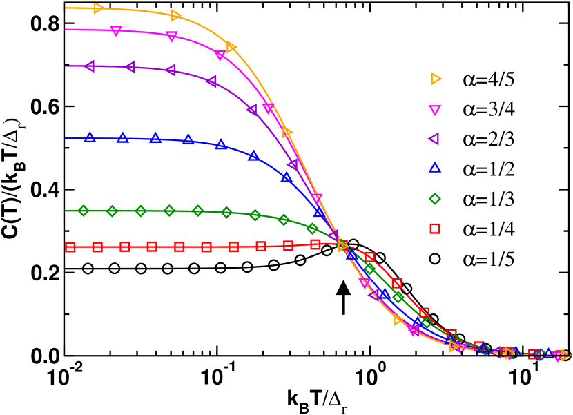
Figure 12: (Color online) Specific heat, $C_{\rm imp}(T)/{k_{\rm B}T/\Delta_{\rm r}}$, of the Ohmic two state system as a function of reduced temperature $k_{B}T/\Delta_{\rm r}$, for a range of dissipation strengths $\alpha=1/5,1/4,1/3,1/2,2/3,3/4,4/5$. Symbols: NRG results in new approach. Lines: Bethe ansatz results. The renormalized tunneling amplitude $\Delta_{\rm r}$ from the Bethe ansatz is used. The vertical arrow indicates the approximate crossing point at $k_{\rm B}T/\Delta_{\rm r}\approx 0.67$. Model parameters: $\Delta_{\rm 0}/\omega_{\rm c}=0.005$. NRG parameters: $\Lambda=10,n_{z}=4$ retaining $860$ states per NRG iteration.

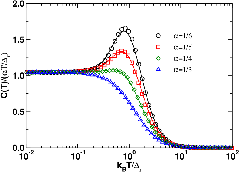
Figure 13: (Color online) Specific heat, $C_{\rm imp}(T)/(\alpha k_{\rm B}T/\Delta_{\rm r})$, of the Ohmic two state system as a function of reduced temperature $k_{B}T/\Delta_{\rm r}$, for a range of dissipation strengths $\alpha<1/2$. Symbols: NRG results in new approach. Lines: Bethe ansatz results. In the low temperature Fermi liquid regime, $T\ll\Delta_{\rm r}$, we have $C_{\rm imp}(T)/(\alpha k_{\rm B}T/\Delta_{\rm r})=\tilde{\gamma}+\tilde{\beta}(T/\Delta_{\rm r})^{2}$, with $\tilde{\gamma}=\pi/3$ and the $T^{3}$ coefficient in $C(T)$ changes sign for $\alpha<1/3$ (see Ref. Costi and Zarand, 1999). Model parameters: $\Delta_{\rm 0}/\omega_{\rm c}=0.005$. NRG parameters: $\Lambda=10,n_{z}=4$ retaining $860$ states per NRG iteration.

VII Discussion and conclusions

In this paper, we introduced a new approach to the calculation of impurity internal energies and specific heats of quantum impurity models within the NRG method. For general Anderson impurity models, the impurity contribution to the internal energy was expressed in terms of local quantities and the main contribution to the impurity specific heat was shown to arise from local static correlation functions. For this class of models, the impurity specific heat can be obtained essentially exactly as $C_{\rm imp}(T)=\frac{\partial E_{\rm ionic}}{\partial T}+\frac{1}{2}\frac{\partial E_{\rm hyb}}{\partial T}$, where $E_{\rm ionic}=\langle H_{\rm imp}\rangle$ and $E_{\rm hyb}$ is the hybridization energy. A comparison with exact Bethe ansatz calculations showed that the results for specific heats of the Anderson impurity model are recovered accurately over the whole temperature and magnetic field range. The new method has several advantages over the conventional approach to specific heats within the NRG, namely, (i), only diagonalization of the total system is required, (ii), only local quantities are required, and, (iii), discretization oscillations at large $\Lambda$ are significantly smaller than in the conventional approach.

For the dissipative two state system we obtain the specific heat as $C_{\rm imp}(T)\equiv\frac{\partial E_{\rm imp}}{\partial T}=\frac{\partial E_{\rm S}}{\partial T}+\frac{\partial E_{\rm B}^{(2)}}{\partial T}$, where $E_{\rm S}=\langle H_{\rm S}\rangle$ is analogous to $E_{\rm ionic}$ in the Anderson model, and $E_{\rm B}^{(2)}$ is a contribution to the energy of the system arising from the interaction with the bath. It depends on the local dynamical susceptibility and the type of coupling to the environment. For the Ohmic case, we used the equivalence of the Ohmic two state system to the AKM to show numerically that $E_{\rm B}^{(2)}=\frac{1}{2}\alpha\Delta_{0}\langle\sigma_{x}\rangle+A$ with $A$ having a negligible temperature dependence, except in the extreme limit $\alpha\rightarrow 1^{-}$. Comparison with exact Bethe ansatz calculations on the AKM confirmed the above.

The approach described in this paper applies to energy dependent hybridizations also, see Fig. 7, so, inclusion of the term $E_{\rm int}^{(2)}$ in Eq. (15), could prove useful in applications to quantum impurities with a pseudogap density of states.Gonzalez-Buxton and Ingersent (1998); Vojta and Bulla (2002) It may also be applied within other methods for solving quantum impurity models, for example, within continuous time Gull et al. (2011) or Hirsch-Fey Hirsch and Fye (1986) quantum Monte Carlo techniques or exact diagonalization methods (for a recent review see Ref. Liebsch and Ishida, 2012 and references therein). Local static correlation functions, such as the double occupancy, required for $E_{\rm imp}$, are readily extracted within these approaches.Jakobi et al. (2009)

Within a DMFT treatment of correlated lattice models, Metzner and Vollhardt (1989); Georges et al. (1996); Kotliar and Vollhardt (2004); Vollhardt (2012) the hybridization function $\Delta$ acquires an important temperature and frequency dependence $\Delta(\omega)\rightarrow\Delta(\omega,T)$. The latter enters explicitly in the term $E_{\rm int}^{(2)}$, whose inclusion could offer an approach to the calulation of specific heats of correlated lattice models. The thermodynamic potential of the latter Janiš (1991) is a sum of two parts, one depending on the local self-energy, which is the central quantity calculated in DMFT, and another equal to the thermodynamic potential, $\Omega_{\rm imp}=E_{\rm imp}-TS_{\rm imp}$, of the effective impurity model. The latter can be obtained from $E_{\rm imp}(T)$, via $C_{\rm imp}(T)$ and $S_{\rm imp}(T)=\int_{0}^{T}dT^{\prime}\frac{C_{\rm imp}(T^{\prime})}{T^{\prime}}$. The impurity internal energy, expressed in terms of local dynamical quantities as in Ref. Kjöllerström et al., 1966, has recently been used in a DMFT solution of the Hubbard model within a variational generalization Kauch and Byczuk (2012) of the local moment approach.Logan et al. (1998)

In the future, it may be interesting, especially in the context of qubits or nanodevices, to consider the time dependence of the impurity internal energy subject to an initial state preparation, for example, within techniques such as time-dependent density matrix renormalization group Daley et al. (2004); White and Feiguin (2004); Dias da Silva et al. (2008) or time-dependent NRG.Costi (1997); Anders and Schiller (2005); Rosch (2012)

Appendix A Band contribution to impurity internal energy

The expression (11) for the conduction band contribution to the impurity internal energy requires evaluation of the integral

$$I(\omega)=\int d\epsilon\frac{\epsilon V^{2}N(\epsilon)}{(\omega-\epsilon+i\delta)^{2}}.$$ (35)

We assume a density of states $N(\omega)$ vanishing at the band edges at $\omega=\pm D$. The hybridization function $\Delta(\omega)=\sum_{k}V^{2}/(\omega-\epsilon_{k}+i\delta)=\Delta_{R}(\omega)+i\Delta_{I}(\omega)$ where $\Delta_{I}(\omega)=-\pi N(\omega)V^{2}$. With these definitions, we have

$$I(\omega) = -\frac{1}{\pi}\int_{-D}^{+D}d\epsilon\epsilon\Delta_{I}(\epsilon)\frac{\partial}{\partial\epsilon}\frac{1}{(\omega-\epsilon+i\delta)}$$ (36)

$$= -\frac{1}{\pi}\frac{\epsilon\Delta_{I}(\epsilon)}{\omega-\epsilon+i\delta}|_{-D}^{+D}$$

$$+\frac{1}{\pi}\int_{-D}^{+D}d\epsilon\frac{1}{\omega-\epsilon+i\delta}\frac{\partial}{\partial\epsilon}(\epsilon\Delta_{I}(\epsilon)).$$

The first term vanishes since $\Delta_{I}(\pm D)=0$ for regular (e.g., $3D$) densities of states (and will otherwise result in contributions with negligible temperature dependence). The second term can be evaluated by noting that $\Delta(\omega+i\delta)$ satisfies the causal properties of retarded Green functions and by using the following properties of principle value (P.V.) integrals: if P.V.[$f(x)$] $=g(y)$ then P.V.[$f^{\prime}(x)$] $=g^{\prime}(y)$ and P.V.[$xf(x)$] $=yg(y)+\frac{1}{\pi}\int dxf(x)$. The final result is

$$I(\omega)=-\frac{\partial}{\partial\omega}(\omega\Delta(\omega))$$ (37)

Appendix B Numerical solution of the Thermodynamic Bethe Ansatz equations

In this Appendix, we summarize the thermodynamic Bethe ansatz (TBA) equations for the Anderson model, which were derived by Okiji and Kawakami Kawakami and Okiji (1981, 1982a); Okiji and Kawakami (1983) and Tsvelick, Filyov, and Wiegmann, Wiegmann and Tsvelick (1983); Tsvelick and Wiegmann (1983); Filyov et al. (1982); Tsvelick and Wiegmann (1982) and provide details of their numerical solution.Rajan et al. (1982); Desgranges (1985); Sacramento and Schlottmann (1991); Costi and Zarand (1999); Takahashi and Shiroishi (2002); Bolech and Andrei (2005) The numerical procedure described applies to both the symmetric and asymmetric Anderson models and in the presence of a finite magnetic field and was used to obtain the results presented in this paper.

B.1 Thermodynamic Bethe Ansatz Equations

The thermodynamic Bethe ansatz (TBA) produces an infinite set of coupled integral equations for the functions $\epsilon(k)$, $\kappa_{n}^{\prime}(\Lambda)$ and $\kappa_{n}(\Lambda)$, $n=1,2,\dots$, describing the charge and spin excitations of the system (Tsvelick and Wiegmann Tsvelick and Wiegmann (1982)):

$$\epsilon(k) -T\cdot\int_{-\infty}^{\infty}s(g(k)-\Lambda)\cdot\ln(f(\kappa_{1}(\Lambda))\mathrm{d}\Lambda=$$

$$\epsilon_{0}(k)-T\cdot\int_{-\infty}^{\infty}s(g(k)-\Lambda)\cdot\ln(f(\kappa^{\prime}_{1}(\Lambda))\mathrm{d}\Lambda$$ (38a)

$$\kappa_{n}(\Lambda) +T\cdot(s*(\ln(f(\kappa_{n+1}))+\ln(f(\kappa_{n-1}))))(\Lambda)=$$

$$\delta_{n,1}\cdot T\cdot\int^{\infty}_{-\infty}s(g(k)-\Lambda)\cdot\ln(f(-\epsilon(k)))\cdot g^{\prime}(k)\,\mathrm{d}k$$ (38b)

$$\kappa^{\prime}_{n}(\Lambda) +T\cdot(s*(\ln(f(\kappa^{\prime}_{n+1}))+\ln(f(\kappa^{\prime}_{n-1}))))(\Lambda)=$$

$$\delta_{n,1}\cdot T\cdot\int^{\infty}_{-\infty}s(g(k)-\Lambda)\cdot\ln(f(\epsilon(k)))\cdot g^{\prime}(k)\,\mathrm{d}k$$ (38c)

where

$$g(k)=\frac{(k-\varepsilon_{d}-\frac{1}{2}U)^{2}}{2\Gamma\mathrm{U}},\quad s(\Lambda)=\frac{1}{2\cosh(\pi\Lambda)},$$

$$f(k)=\frac{1}{1+\mathrm{e}^{k/T}},\quad R(x)=\frac{1}{\pi}\int_{0}^{\infty}\frac{\cos(\omega x)}{1+\mathrm{e}^{\omega}}\mathrm{d}\omega$$

$$\epsilon_{0}(k)=k-\varepsilon_{d}-\frac{1}{2}U+\int_{-\infty}^{\infty}R(g(k)-g(p))\cdot p\cdot g^{\prime}(p)\mathrm{d}p$$

$g^{\prime}(k)$ denotes the first derivative of $g(k)$ with respect to $k$. $*$ is the convolution of two functions. $\kappa_{0}$ and $\kappa^{\prime}_{0}$ equal $-\infty$. For $n\rightarrow\infty$ the functions approach the constant values,

$$\lim\limits_{n\rightarrow\infty}\kappa_{n}=n\cdot H,\qquad\lim\limits_{n\rightarrow\infty}\kappa^{\prime}_{n}=n\cdot(2\varepsilon_{d}+U),$$ (39)

where $H$ is a uniform magnetic field and $2\varepsilon_{d}+U$ measures the deviation from the symmetric point at $\varepsilon_{d}=-U/2$. The impurity contribution to the specific heat, $C_{\rm imp}$, may be calculated from the the impurity contribution to the thermodynamic potential, $\Omega_{\rm imp}$, via $C_{\rm imp}=-T\partial^{2}\Omega_{\rm imp}/\partial T^{2}$, where

$$\Omega_{\rm imp}= T\int_{-\infty}^{\infty}\rho_{0}(k)\cdot\ln(f(-\epsilon(k)))\mathrm{d}k$$

$$+T\int_{-\infty}^{\infty}\sigma_{0}(\Lambda)\cdot\ln(\kappa^{\prime}_{1}(\Lambda))\mathrm{d}\Lambda+E_{\rm 0}$$ (40)

The functions $\rho_{0}$ and $\sigma_{0}$ are given by:

$$\sigma_{0}(\Lambda) =\int_{-\infty}^{\infty}s(\Lambda-g(k))\cdot\Delta(k)\mathrm{d}k$$

$$\rho_{0}(k) =\Delta(k)+g^{\prime}(k)\cdot\int_{-\infty}^{\infty}R(g(k)-g(p))\cdot\Delta(p)\mathrm{d}p,$$

where $\Delta(k)=\frac{\Gamma}{\pi(\Gamma^{2}+(k-\varepsilon_{d})^{2})}$. $E_{\rm 0}$ is the ground state energy of the symmetric Anderson model.Kawakami and Okiji (1981, 1981) Note two changes with respect to the earlier Ref. Tsvelick and Wiegmann, 1982: a sign change in equation 38c (as in Wiegmann and Tsvelick Wiegmann and Tsvelick (1983)) and a factor $2$ in the boundary value for $\kappa^{\prime}_{n}$ in equation 39 (as in Okiji and Kawakami Okiji and Kawakami (1983)).

For the calculations we use a transformation of $\kappa_{n}$ and $\kappa_{n}^{\prime}$ to new functions $\xi_{n}$ and $\xi_{n}^{\prime}$ similar to that used in previous works.Rajan et al. (1982); Desgranges (1985); Costi and Zarand (1999) After substituting $\xi_{n}=\ln(1+\mathrm{e}^{\kappa_{n}/T})$ and $\xi^{\prime}_{n}=\ln(1+\mathrm{e}^{\kappa^{\prime}_{n}/T})$ we obtain the following coupled equations:

$$\xi_{1}(\Lambda) =\ln(1+\exp((s*(\xi_{2}+I_{1}))(\Lambda)))$$ (41a)

$$\xi_{n}(\Lambda) =\ln(1+\exp((s*(\xi_{n-1}+\xi_{n+1}))(\Lambda)))$$ (41b)

$$\xi^{\prime}_{1}(\Lambda) =\ln(1+\exp((s*(\xi^{\prime}_{2}+I^{\prime}_{1}))(\Lambda)))$$ (41c)

$$\xi^{\prime}_{n}(\Lambda) =\ln(1+\exp((s*(\xi^{\prime}_{n-1}+\xi^{\prime}_{n+1}))(\Lambda)))$$ (41d)

$$I_{1}(\Lambda) =\int^{\infty}_{-\infty}s(g(k)-\Lambda)\cdot\ln(f(-\epsilon(k)))\cdot g^{\prime}(k)\,\mathrm{d}k$$ (41e)

$$I^{\prime}_{1}(\Lambda) =\int^{\infty}_{-\infty}s(g(k)-\Lambda)\cdot\ln(f(\epsilon(k)))\cdot g^{\prime}(k)\,\mathrm{d}k$$ (41f)

$$I(k) =\int_{-\infty}^{\infty}s(g(k)-\Lambda)\cdot(\xi_{1}(\Lambda)-\xi^{\prime}_{1}(\Lambda))\mathrm{d}\Lambda$$ (41g)

$$e(k) =e_{0}(k)+T\cdot I(k)$$ (41h)

B.2 Truncation

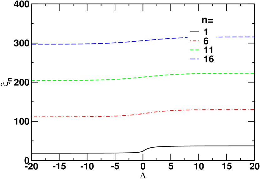
Figure 14: (Color online) The figure shows a set of $\xi_{n}$ for the symmetric case ($\varepsilon_{d}+U/2=0$) zoomed to range of $\Lambda=-20\dots 20$. The functions become smoother with higher $n$ due to the convolution with $s(x)$.

For calculational purposes the equations $\xi_{n}$ and $\xi^{\prime}_{n^{\prime}}$ have to be truncated at some finite value $n=N$ and $n^{\prime}=N^{\prime}$. One has to calculate the functions at the truncation with care, to avoid wrong results at the boundaries $\Lambda\rightarrow\pm\infty$. We use the truncation scheme of Takahashi and Shiroishi.Takahashi and Shiroishi (2002) It is assumed that the function $s(x)$ can be approximated by $\delta(x)/2$ for large $n$ or $n^{\prime}$. This is justified as the functions become smoother in this region (see figure 14). Rewritten for the Anderson Model and for $\xi_{N}$ and $\xi^{\prime}_{N}$ the corresponding truncation functions are calculated by:

$$\xi_{N} =\ln\Big{(}\big{(}\cosh(\frac{H}{2})\cdot\sqrt{2+\mathrm{e}^{\xi_{N-1}}}+$$

$$\qquad\sqrt{1+\sinh^{2}(\frac{H}{2})\cdot[2+\mathrm{e}^{\xi_{N-1}}]}\big{)}^{2}\Big{)}$$ (42a)

$$\xi^{\prime}_{N^{\prime}} =\ln\Big{(}\big{(}\cosh(\frac{2\varepsilon_{d}+U}{2})\cdot\sqrt{2+\mathrm{e}^{\xi^{\prime}_{N^{\prime}-1}}}+$$

$$\qquad\sqrt{1+\sinh^{2}(\frac{2\varepsilon_{d}+U}{2})\cdot[2+\mathrm{e}^{\xi^{\prime}_{N^{\prime}-1}}]}\big{)}^{2}\Big{)}$$ (42b)

As a further check, and to ensure the correct behaviour at the boundaries, the TBA integral equations were explicitly solved in the limits of $\Lambda,k\rightarrow\pm\infty$. As the functions are smooth in this limit one can assume that $s(x)\rightarrow\delta(x)/2$ and $\lim\limits_{k\rightarrow\infty}\epsilon_{0}(k)=2(k-\varepsilon_{d}-U/2)$, $\lim\limits_{k\rightarrow-\infty}\epsilon_{0}(k)=0$. This leads to the following set of coupled algebraic equations:

$$\lim\limits_{\Lambda\rightarrow-\infty}$$

$$\xi_{1} =\ln(1+\exp(\frac{1}{2}\xi_{2})))$$ (43a)

$$\xi_{n} =\ln(1+\exp(\frac{1}{2}(\xi_{n-1}+\xi_{n+1})))$$ (43b)

$$\xi^{\prime}_{1} =\ln(1+\exp(\frac{1}{2}\xi^{\prime}_{2}))$$ (43c)

$$\xi^{\prime}_{n} =\ln(1+\exp(\frac{1}{2}(\xi^{\prime}_{n-1}+\xi^{\prime}_{n+1})))$$ (43d)

$$\lim\limits_{\Lambda\rightarrow\infty}$$

$$\xi_{1} =\ln(1+\exp(\frac{1}{2}(\xi_{2}-\ln(1+\exp(\frac{1}{2}\xi_{1})))))$$ (43e)

$$\xi_{n} =\ln(1+\exp(\frac{1}{2}(\xi_{n-1}+\xi_{n+1})))$$ (43f)

$$\xi^{\prime}_{1} =0$$ (43g)

$$\xi^{\prime}_{n} =\ln(1+\exp(\frac{1}{2}(\xi^{\prime}_{n-1}+\xi^{\prime}_{n+1})))$$ (43h)

The truncation constants $\xi_{N}$ and $\xi^{\prime}_{N^{\prime}}$ are calculated as in equation 42. The boundary values where calculated by iteration using a modification of the Powell hybrid method.

B.3 Numerical Details

For the calculations, a logarithmic grid was used that is centred around $\varepsilon_{d}+U/2$. The TBA equations were solved by iteration. The initial values of $\xi_{n}$ and $\xi^{\prime}_{n^{\prime}}$ were chosen to fit a $\tanh$-function with boundary values given by the correct boundary values of $\xi_{n}$ and $\xi^{\prime}_{n}$, obtained as described above. The integrations were carried out using adaptive routines with the integrands being represented by splines of smooth functions only (see below). A smoother convergence of the iteration procedure is obtained by using $10\%$ of the old iteration values in each step. To represent only smooth functions as splines, $\xi_{1}$ and $\xi^{\prime}_{1}$ are not interpolated, but instead the $s*\xi_{2}$ and $s*\xi^{\prime}_{2}$ respectively. The values of $\xi_{1}$ and $\xi^{\prime}_{1}$ are then calculated from these convolutions and from $I_{1}$ and $I^{\prime}_{1}$ using Eq. (41a) and Eq. (41c). This avoids numerical problems due to the exponential drop to zero of $\xi_{1}^{\prime}$ beyond a certain rapidity $\Lambda_{0}$. See Figure 15 for a comparison between the behavior of $\xi^{\prime}_{1}$ and $I^{\prime}_{1}$.

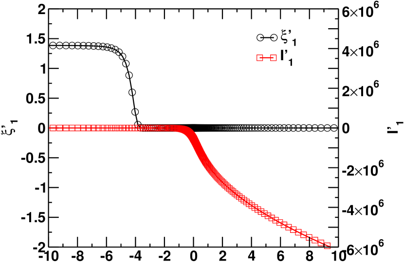
Figure 15: (Color online) Comparison between $I^{\prime}_{1}$ and $\xi^{\prime}_{1}$ for 500 iterations and $T=10^{-4}T_{K}$. Parameters were chosen to be the same as in figure 1. For very low temperatures $\xi^{\prime}_{1}$ (circles, left $y$-axis) exhibits an exponential drop beyond a certain rapidity $\Lambda_{0}$ ($\approx-4$ for the case shown) which is difficult to capture with a fixed grid. This problem can be overcome by using the smooth function $I_{1}^{\prime}$ (squares, right $y$-axis) to calculate $\xi_{1}^{\prime}$ via Eq. (41c).

$N=N^{\prime}=20$ functions were used and iterated $500$ times for the figures in this section (and $2000$ times for the results in the paper). The growth-rate of the grid was $1.05$ and it consisted of 801 points. The mid 400 values lie in a range of $[-40,40]$. After a certain temperature dependent cut-off ($\pm 40\pm 40\cdot T/T_{0}$) the boundary values were used instead of being calculated to ensure numerical stability. The thermodynamic potential was calculated in a range of $T_{0}\cdot 10^{-3}$ to $T_{0}\cdot 10^{6}$ on a logarithmic mesh (factor $2^{1/8}$ as step width) where $T_{0}$ is defined as $T_{0}=\sqrt{U\Gamma/2}\cdot\exp(-\frac{\pi U}{8\Gamma}+\frac{\pi\Gamma}{2U})$, Kondo temperature for the symmetric case. It is related to the magnetic susceptibility at zero temperature $\chi_{\rm imp}(T=0)=\frac{(g\mu_{\rm B})^{2}}{4k_{\rm B}T_{0}}$ (see Hewson in Ref. Hewson, 1997 p. 165, and Kawakami and Okiji in Ref. Kawakami and Okiji, 1982b).

References

- Hewson (1997) A. C. Hewson, The Kondo Problem to Heavy Fermions (Cambridge University Press, Cambridge, 1997).
- Zawadowski (1980) A. Zawadowski, Phys. Rev. Lett. 45, 211 (1980).
- Caldeira and Leggett (1983) A. Caldeira and A. Leggett, Annals of Physics 149, 374 (1983).
- Leggett et al. (1987) A. J. Leggett, S. Chakravarty, A. T. Dorsey, M. P. A. Fisher, A. Garg, and W. Zwerger, Rev. Mod. Phys. 59, 1 (1987).
- Weiss (2008) U. Weiss, Quantum dissipative systems, Vol. 13 (World Scientific Pub Co Inc, 2008).
- Zaránd (2005) G. Zaránd, Phys. Rev. B 72, 245103 (2005).
- Loss and DiVincenzo (1998) D. Loss and D. P. DiVincenzo, Phys. Rev. A 57, 120 (1998).
- Park et al. (2002) J. Park, A. Pasupathy, J. Goldsmith, C. Chang, Y. Yaish, J. Petta, M. Rinkoski, J. Sethna, H. Abruna, P. McEuen, and D. Ralph, Nature 417, 722 (2002).
- Yu and Natelson (2004) L. H. Yu and D. Natelson, Nano Letters 4, 79 (2004).
- Roch et al. (2009) N. Roch, S. Florens, T. A. Costi, W. Wernsdorfer, and F. Balestro, Phys. Rev. Lett. 103, 197202 (2009).
- Parks et al. (2010) J. J. Parks, A. R. Champagne, T. A. Costi, W. W. Shum, A. N. Pasupathy, E. Neuscamman, S. Flores-Torres, P. S. Cornaglia, A. A. Aligia, C. A. Balseiro, G. K.-L. Chan, H. D. Abruña, and D. C. Ralph, Science 328, 1370 (2010).
- Goldhaber-Gordon et al. (1998) D. Goldhaber-Gordon, J. Göres, M. A. Kastner, H. Shtrikman, D. Mahalu, and U. Meirav, Phys. Rev. Lett. 81, 5225 (1998).
- Cronenwett et al. (1998) S. M. Cronenwett, T. H. Oosterkamp, and L. P. Kouwenhoven, Science 281, 540 (1998).
- Kretinin et al. (2011) A. V. Kretinin, H. Shtrikman, D. Goldhaber-Gordon, M. Hanl, A. Weichselbaum, J. von Delft, T. Costi, and D. Mahalu, Phys. Rev. B 84, 245316 (2011).
- Nygard et al. (2000) J. Nygard, D. Cobden, and P. Lindelof, Nature 408, 342 (2000).
- Madhavan et al. (1998) V. Madhavan, W. Chen, T. Jamneala, M. Crommie, and N. Wingreen, Science 280, 567 (1998).
- Otte et al. (2008) A. Otte, M. Ternes, K. Von Bergmann, S. Loth, H. Brune, C. Lutz, C. Hirjibehedin, and A. Heinrich, Nature Physics 4, 847 (2008).
- Li et al. (1998) J. Li, W.-D. Schneider, R. Berndt, and B. Delley, Phys. Rev. Lett. 80, 2893 (1998).
- Metzner and Vollhardt (1989) W. Metzner and D. Vollhardt, Phys. Rev. Lett. 62, 324 (1989).
- Georges et al. (1996) A. Georges, G. Kotliar, W. Krauth, and M. J. Rozenberg, Rev. Mod. Phys. 68, 13 (1996).
- Kotliar and Vollhardt (2004) G. Kotliar and D. Vollhardt, Physics Today 57, 53 (2004).
- Vollhardt (2012) D. Vollhardt, Annalen der Physik 524, 1 (2012).
- Wilson (1975) K. G. Wilson, Rev. Mod. Phys. 47, 773 (1975).
- Krishna-murthy et al. (1980a) H. R. Krishna-murthy, J. W. Wilkins, and K. G. Wilson, Phys. Rev. B 21, 1003 (1980a).
- Krishna-murthy et al. (1980b) H. R. Krishna-murthy, J. W. Wilkins, and K. G. Wilson, Phys. Rev. B 21, 1044 (1980b).
- Bulla et al. (2008) R. Bulla, T. A. Costi, and T. Pruschke, Rev. Mod. Phys. 80, 395 (2008).
- Oliveira and Wilkins (1981) L. N. Oliveira and J. W. Wilkins, Phys. Rev. Lett. 47, 1553 (1981).
- Frota and Oliveira (1986) H. O. Frota and L. N. Oliveira, Phys. Rev. B 33, 7871 (1986).
- Sakai et al. (1989) O. Sakai, Y. Shimizu, and T. Kasuya, Journal of the Physical Society of Japan 58, 3666 (1989).
- Costi and Hewson (1992) T. A. Costi and A. C. Hewson, Philosophical Magazine Part B 65, 1165 (1992).
- Bulla et al. (1998) R. Bulla, A. C. Hewson, and T. Pruschke, Journal of Physics: Condensed Matter 10, 8365 (1998).
- Hofstetter (2000) W. Hofstetter, Phys. Rev. Lett. 85, 1508 (2000).
- Anders and Schiller (2005) F. B. Anders and A. Schiller, Phys. Rev. Lett. 95, 196801 (2005).
- Peters et al. (2006) R. Peters, T. Pruschke, and F. B. Anders, Phys. Rev. B 74, 245114 (2006).
- Weichselbaum and von Delft (2007) A. Weichselbaum and J. von Delft, Phys. Rev. Lett. 99, 076402 (2007).
- Costi et al. (1994) T. A. Costi, A. C. Hewson, and V. Zlatić, J. Phys.: Condens. Matter 6, 2519 (1994).
- Gonzalez-Buxton and Ingersent (1998) C. Gonzalez-Buxton and K. Ingersent, Phys. Rev. B 57, 14254 (1998).
- Löhneysen et al. (2007) H. v. Löhneysen, A. Rosch, M. Vojta, and P. Wölfle, Rev. Mod. Phys. 79, 1015 (2007).
- Costa et al. (1997) S. C. Costa, C. A. Paula, V. L. Líbero, and L. N. Oliveira, Phys. Rev. B 55, 30 (1997).
- Tsvelick and Wiegmann (1982) A. M. Tsvelick and P. B. Wiegmann, Physics Letters A 89, 368 (1982).
- Wiegmann and Tsvelick (1983) P. B. Wiegmann and A. M. Tsvelick, Journal of Physics C: Solid State Physics 16, 2281 (1983).
- Okiji and Kawakami (1983) A. Okiji and N. Kawakami, Phys. Rev. Lett. 50, 1157 (1983).
- Nagaoka (1965) Y. Nagaoka, Phys. Rev. 138, A1112 (1965).
- Bloomfield and Hamann (1967) P. E. Bloomfield and D. R. Hamann, Phys. Rev. 164, 856 (1967).
- Kjöllerström et al. (1966) B. Kjöllerström, D. J. Scalapino, and J. R. Schrieffer, Phys. Rev. 148, 665 (1966).
- Rajan et al. (1982) V. T. Rajan, J. H. Lowenstein, and N. Andrei, Phys. Rev. Lett. 49, 497 (1982).
- Desgranges (1985) H.-U. Desgranges, Journal of Physics C: Solid State Physics 18, 5481 (1985).
- Sacramento and Schlottmann (1991) P. D. Sacramento and P. Schlottmann, Phys. Rev. B 43, 13294 (1991).
- Bolech and Andrei (2005) C. J. Bolech and N. Andrei, Phys. Rev. B 71, 205104 (2005).
- Oliveira and Oliveira (1994) W. C. Oliveira and L. N. Oliveira, Phys. Rev. B 49, 11986 (1994).
- Campo and Oliveira (2005) V. L. Campo and L. N. Oliveira, Phys. Rev. B 72, 104432 (2005).
- Silva et al. (1996) J. B. Silva, W. L. C. Lima, W. C. Oliveira, J. L. N. Mello, L. N. Oliveira, and J. W. Wilkins, Phys. Rev. Lett. 76, 275 (1996).
- Campo and Oliveira (2004) V. L. Campo and L. N. Oliveira, Phys. Rev. B 70, 153401 (2004).
- Ferreira et al. (2012) J. V. B. Ferreira, A. I. I. Ferreira, A. H. Leite, and V. L. Líbero, Journal of Magnetism and Magnetic Materials 324, 1011 (2012).
- Anderson (1961) P. W. Anderson, Physical Review 124, 41 (1961).
- Schrieffer and Wolff (1966) J. R. Schrieffer and P. A. Wolff, Phys. Rev. 149, 491 (1966).
- Iche and Zawadowski (1972) G. Iche and A. Zawadowski, Solid State Communications 10, 1001 (1972).
- Hewson et al. (2006) A. C. Hewson, J. Bauer, and W. Koller, Phys. Rev. B 73, 045117 (2006).
- Ramos et al. (2003) L. R. Ramos, W. C. Oliveira, and V. L. Líbero, Phys. Rev. B 67, 085104 (2003).
- Guinea et al. (1985) F. Guinea, V. Hakim, and A. Muramatsu, Phys. Rev. B 32, 4410 (1985).
- Costi and Kieffer (1996) T. A. Costi and C. Kieffer, Phys. Rev. Lett. 76, 1683 (1996).
- Costi and Zarand (1999) T. A. Costi and G. Zarand, Physical Review B 59, 12398 (1999).
- Costi (1998) T. A. Costi, Phys. Rev. Lett. 80, 1038 (1998).
- Görlich and Weiss (1988) R. Görlich and U. Weiss, Phys. Rev. B 38, 5245 (1988).
- Chandra et al. (1999) N. Chandra, M. Kollar, and D. Vollhardt, Phys. Rev. B 59, 10541 (1999).
- Costi and McKenzie (2003) T. A. Costi and R. H. McKenzie, Phys. Rev. A 68, 034301 (2003).
- Hur (2008) K. L. Hur, Annals of Physics 323, 2208 (2008).
- Florens et al. (2011) S. Florens, A. Freyn, D. Venturelli, and R. Narayanan, Phys. Rev. B 84, 155110 (2011).
- Hänggi and Ingold (2006) P. Hänggi and G.-L. Ingold, Acta Physica Plolonica B 37, 1537 (2006).
- Hänggi et al. (2008) P. Hänggi, G.-L. Ingold, and P. Talkner, New Journal of Physics 10, 115008 (2008).
- Ingold et al. (2009) G.-L. Ingold, P. Hänggi, and P. Talkner, Phys. Rev. E 79, 061105 (2009).
- Ingold (2012) G. Ingold, The European Physical Journal B-Condensed Matter and Complex Systems 85, 1 (2012).
- Ford and O’Connell (2005) G. W. Ford and R. F. O’Connell, Physica E: Low-dimensional Systems and Nanostructures 29, 82 (2005).
- Hasegawa (2011) H. Hasegawa, Journal of Mathematical Physics 52, 123301 (2011).
- Callen (1985) H. B. Callen, Thermodynamics and an Introduction to Thermostatistics (John Wiley & Sons, New York, 1985).
- Florens and Rosch (2004) S. Florens and A. Rosch, Phys. Rev. Lett. 92, 216601 (2004).
- Žitko and Pruschke (2009) R. Žitko and T. Pruschke, Phys. Rev. B 79, 012507 (2009).
- Vojta and Bulla (2002) M. Vojta and R. Bulla, The European Physical Journal B-Condensed Matter and Complex Systems 28, 283 (2002).
- Gull et al. (2011) E. Gull, A. J. Millis, A. I. Lichtenstein, A. N. Rubtsov, M. Troyer, and P. Werner, Rev. Mod. Phys. 83, 349 (2011).
- Hirsch and Fye (1986) J. E. Hirsch and R. M. Fye, Phys. Rev. Lett. 56, 2521 (1986).
- Liebsch and Ishida (2012) A. Liebsch and H. Ishida, Journal of Physics: Condensed Matter 24, 053201 (2012).
- Jakobi et al. (2009) E. Jakobi, N. Blümer, and P. van Dongen, Phys. Rev. B 80, 115109 (2009).
- Janiš (1991) V. Janiš, Zeitschrift für Physik B Condensed Matter 83, 227 (1991).
- Kauch and Byczuk (2012) A. Kauch and K. Byczuk, Physica B: Condensed Matter 407, 209 (2012).
- Logan et al. (1998) D. E. Logan, M. P. Eastwood, and M. A. Tusch, Journal of Physics: Condensed Matter 10, 2673 (1998).
- Daley et al. (2004) A. J. Daley, C. Kollath, U. Schollwöck, and G. Vidal, Journal of Statistical Mechanics: Theory and Experiment 2004, P04005 (2004).
- White and Feiguin (2004) S. R. White and A. E. Feiguin, Phys. Rev. Lett. 93, 076401 (2004).
- Dias da Silva et al. (2008) L. G. G. V. Dias da Silva, F. Heidrich-Meisner, A. E. Feiguin, C. A. Büsser, G. B. Martins, E. V. Anda, and E. Dagotto, Phys. Rev. B 78, 195317 (2008).
- Costi (1997) T. A. Costi, Phys. Rev. B 55, 3003 (1997).
- Rosch (2012) A. Rosch, The European Physical Journal B-Condensed Matter and Complex Systems 85, 1 (2012).
- Kawakami and Okiji (1981) N. Kawakami and A. Okiji, Physics Letters A 86, 483 (1981).
- Kawakami and Okiji (1982a) N. Kawakami and A. Okiji, Journal of the Physical Society of Japan 51, 2043 (1982a).
- Tsvelick and Wiegmann (1983) A. M. Tsvelick and P. B. Wiegmann, Journal of Physics C: Solid State Physics 16, 2321 (1983).
- Filyov et al. (1982) V. M. Filyov, A. M. Tsvelick, and P. B. Wiegmann, Physics Letters A 89, 157 (1982).
- Takahashi and Shiroishi (2002) M. Takahashi and M. Shiroishi, Phys. Rev. B 65, 165104 (2002).
- Kawakami and Okiji (1982b) N. Kawakami and A. Okiji, Solid State Communications 43, 467 (1982b).