Software Model Checking with Explicit Scheduler and Symbolic Threads

Abstract.

In many practical application domains, the software is organized into a set of threads, whose activation is exclusive and controlled by a cooperative scheduling policy: threads execute, without any interruption, until they either terminate or yield the control explicitly to the scheduler.

The formal verification of such software poses significant challenges. On the one side, each thread may have infinite state space, and might call for abstraction. On the other side, the scheduling policy is often important for correctness, and an approach based on abstracting the scheduler may result in loss of precision and false positives. Unfortunately, the translation of the problem into a purely sequential software model checking problem turns out to be highly inefficient for the available technologies.

We propose a software model checking technique that exploits the intrinsic structure of these programs. Each thread is translated into a separate sequential program and explored symbolically with lazy abstraction, while the overall verification is orchestrated by the direct execution of the scheduler. The approach is optimized by filtering the exploration of the scheduler with the integration of partial-order reduction.

The technique, called ESST (Explicit Scheduler, Symbolic Threads) has been implemented and experimentally evaluated on a significant set of benchmarks. The results demonstrate that ESST technique is way more effective than software model checking applied to the sequentialized programs, and that partial-order reduction can lead to further performance improvements.

1. Introduction

In many practical application domains, the software is organized into a set of threads that are activated by a scheduler implementing a set of domain-specific rules. Particularly relevant is the case of multi-threaded programs with cooperative scheduling, shared-variables and with mutually-exclusive thread execution. With cooperative scheduling, there is no preemption: a thread executes, without interruption, until it either terminates or explicitly yields the control to the scheduler. This programming model, simply called cooperative threads in the following, is used in several software paradigms for embedded systems (e.g.,  SystemC [Ope05], FairThreads [Bou06], OSEK/VDX [OSE05], SpecC [GDPG01]), and also in other domains (e.g., [CGM⁺98]).

Such applications are often critical, and it is thus important to provide highly effective verification techniques. In this paper, we consider the use of formal techniques for the verification of cooperative threads. We face two key difficulties: on the one side, we must deal with the potentially infinite state space of the threads, which often requires the use of abstractions; on the other side, the overall correctness often depends on the details of the scheduling policy, and thus the use of abstractions in the verification process may result in false positives.

Unfortunately, the state of the art in verification is unable to deal with such challenges. Previous attempts to apply various software model checking techniques to cooperative threads (in specific domains) have demonstrated limited effectiveness. For example, techinques like [KS05, TCMM07, CJK07] abstract away significant aspects of the scheduler and synchronization primitives, and thus they may report too many false positives, due to loss of precision, and their applicability is also limited. Symbolic techniques, like [MMMC05, HFG08], show poor scalability because too many details of the scheduler are included in the model. Explicit-state techniques, like [CCNR11], are effective in handling the details of the scheduler and in exploring possible thread interleavings, but are unable to counter the infinite nature of the state space of the threads [GV04]. Unfortunately, for explicit-state techniques, a finite-state abstraction is not easily available in general.

Another approach could be to reduce the verification of cooperative threads to the verification of sequential programs. This approach relies on a translation from (or sequentialization of) the cooperative threads to the (possibly non-deterministic) sequential programs that contain both the mapping of the threads in the form of functions and the encoding of the scheduler. The sequentialized program can be analyzed by means of “off-the-shelf” software model checking techniques, such as [CKSY05, McM06, BHJM07], that are based on the counter-example guided abstraction refinement (CEGAR) [CGJ⁺03] paradigm. However, this approach turns out to be problematic. General purpose analysis techniques are unable to exploit the intrinsic structures of the combination of scheduler and threads, hidden by the translation into a single program. For instance, abstraction-based techniques are inefficient because the abstraction of the scheduler is often too aggressive, and many refinements are needed to re-introduce necessary details.

In this paper we propose a verification technique which is tailored to the verification of cooperative threads. The technique translates each thread into a separate sequential program; each thread is analyzed, as if it were a sequential program, with the lazy predicate abstraction approach [HJMS02, BHJM07]. The overall verification is orchestrated by the direct execution of the scheduler, with techniques similar to explicit-state model checking. This technique, in the following referred to as Explicit-Scheduler/Symbolic Threads (ESST) model checking, lifts the lazy predicate abstraction for sequential software to the more general case of multi-threaded software with cooperative scheduling.

Furthermore, we enhance ESST with partial-order reduction [God96, Pel93, Val91]. In fact, despite its relative effectiveness, ESST often requires the exploration of a large number of thread interleavings, many of which are redundant, with subsequent degradations in the run time performance and high memory consumption [CMNR10]. POR essentially exploits the commutativity of concurrent transitions that result in the same state when they are executed in different orders. We integrate within ESST two complementary POR techniques, persistent sets and sleep sets. The POR techniques in ESST limit the expansion of the transitions in the explicit scheduler, while leave the nature of the symbolic analysis of the threads unchanged. The integration of POR in ESST algorithm is only seemingly trivial, because POR could in principle interact negatively with the lazy predicate abstraction used for analyzing the threads.

The ESST algorithm has been implemented within the Kratos software model checker [CGM⁺11]. Kratos has a generic structure, encompassing the cooperative threads framework, and has been specialized for the verification of SystemC programs [Ope05] and of FairThreads programs [Bou06]. Both SystemC and FairThreads fall within the paradigm of cooperative threads, but they have significant differences. This indicates that the ESST approach is highly general, and can be adapted to specific frameworks with moderate effort. We carried out an extensive experimental evaluation over a significant set of benchmarks taken and adapted from the literature. We first compare ESST with the verification of sequentialized benchmarks, and then analyze the impact of partial-order reduction. The results clearly show that ESST dramatically outperforms the approach based on sequentialization, and that both POR techniques are very effective in further boosting the performance of ESST.

This paper presents in a general and coherent manner material from [CMNR10] and from [CNR11]. While in [CMNR10] and in  [CNR11] the focus is on SystemC, the framework presented in this paper deals with the general case of cooperative threads, without focussing on a specific programming framework. In order to emphasize the generality of the approach, the experimental evaluation in this paper has been carried out in a completely different setting than the one used in [CMNR10] and in [CNR11], namely the FairThreads programming framework. We also considered a set of new benchmarks from [Bou06] and from [WH08], in addition to adapting some of the benchmarks used in [CNR11] to the FairThreads scheduling policy. We also provide proofs of correctness of the proposed techniques in Appendix A.

The structure of this paper is as follows. Section 2 provides some background in software model checking via the lazy predicate abstraction. Section 3 introduces the programming model to which ESST can be applied. Section 4 presents the ESST algorithm. Section 5 explains how to extend ESST with POR techniques. Section 6 shows the experimental evaluation. Section 7 discusses some related work. Finally, Section 8 draws conclusions and outlines some future work.

2. Background

In this section we provide some background on software model checking via the lazy predicate abstraction for sequential programs.

2.1. Sequential Programs

We consider sequential programs written in a simple imperative programming language over a finite set $\mathit{Var}$ of integer variables, with basic control-flow constructs (e.g., sequence, if-then-else, iterative loops) where each operation is either an assignment or an assumption. An assignment is of the form $x:=exp$, where $x$ is a variable and $exp$ is either a variable, an integer constant, an explicit nondeterministic construct $*$, or an arithmetic operation. To simplify the presentation, we assume that the considered programs do not contain function calls. Function calls can be removed by inlining, under the assumption that there are no recursive calls (a typical assumption in embedded software). An assumption is of the form $[bexp]$, where $bexp$ is a Boolean expression that can be a relational operation or an operation involving Boolean operators. Subsequently, we denote by $Ops$ the set of program operations.

Without loss of generality, we represent a program $P$ by a control-flow graph (CFG). [Control-Flow Graph] A control-flow graph $G$ for a program $P$ is a tuple $(L,E,l_{0},L_{err})$ where

1. $L$ is the set of program locations,

2. $E\subseteq L\times Ops\times L$ is the set of directed edges labelled by a program operation from the set $Ops$,

3. $l_{0}\in L$ is the unique entry location such that, for any location $l\in L$ and any operation $op\in Ops$, the set $E$ does not contain any edge $(l,op,l_{0})$, and

4. $L_{err}\subseteq L$ of is the set of error locations such that, for each $l_{e}\in L_{err}$, we have $(l_{e},op,l)\not\in E$ for all $op\in Ops$ and for all $l\in L$.

In this paper we are interested in verifying safety properties by reducing the verification problem to the reachability of error locations.

Figure 1. An example of a
control-flow graph.

Figure 1 depicts an example of a CFG. Typical program assertions can be represented by branches going to error locations. For example, the branches going out of $l_{6}$ can be the representation of assert(y >= 0).

A state $s$ of a program is a mapping from variables to their values (in this case integers). Let $\mathit{State}$ be the set of states, we have $s\in\mathit{State}=\mathit{Var}\rightarrow\mathbb{Z}.$ We denote by $\mathit{Dom}(s)$ the domain of a state $s$. We also denote by $s[x_{1}\mapsto v_{1},\ldots,x_{n}\mapsto v_{n}]$ the state obtained from $s$ by substituting the image of $x_{i}$ in $s$ by $v_{i}$ for all $i=1,\ldots,n$. Let $G=(L,E,l_{0},L_{err})$ be the CFG for a program $P$. A configuration $\gamma$ of $P$ is a pair $(l,s)$, where $l\in L$ and $s$ is a state. We assume some first-order language in which one can represent a set of states symbolically. We write $s\models\varphi$ to mean the formula $\varphi$ is true in the state $s$, and also say that $s$ satisfies $\varphi$, or that $\varphi$ holds at $s$. A data region $r\subseteq\mathit{State}$ is a set of states. A data region $r$ can be represented symbolically by a first-order formula $\varphi_{r}$, with free variables from $\mathit{Var}$, such that all states in $r$ satisfy $\varphi_{r}$; that is, $r=\{s\mid s\models\varphi_{r}\}$. When the context is clear, we also call the formula $\varphi_{r}$ data region as well. An atomic region, or simply a region, is a pair $(l,\varphi)$, where $l\in L$ and $\varphi$ is a data region, such that the pair represents the set $\{(l,s)\mid s\models\varphi\}$ of program configurations. When the context is clear, we often refer to the both kinds of region as simply region.

The semantics of an operation $op\in Ops$ can be defined by the strongest post-operator $\mathit{SP}_{op}$. For a formula $\varphi$ representing a region, the strongest post-condition $\mathit{SP}_{op}(\varphi)$ represents the set of states that are reachable from any of the states in the region represented by $\varphi$ after the execution of the operation $op$. The semantics of assignment and assumption operations are as follows:

$$\begin{array}[]{rcl}\mathit{SP}_{x:=exp}(\varphi)&=&\exists x^{\prime}.\varphi[x/x^{\prime}]\and(x=exp[x/x^{\prime}])\mbox{, for $exp\neq*$,}\\ \mathit{SP}_{x:=*}(\varphi)&=&\exists x^{\prime}.\varphi[x/x^{\prime}]\and(x=a)\mbox{, where $a$ is a fresh variable, and}\\ \mathit{SP}_{[bexp]}(\varphi)&=&\varphi\and bexp,\end{array}$$

where $\varphi[x/x^{\prime}]$ and $exp[x/x^{\prime}]$, respectively, denote the formula obtained from $\varphi$ and the expression obtained from $exp$ by replacing the variable $x^{\prime}$ for $x$. We define the application of the strongest post-operator to a finite sequence $\sigma=op_{1},\ldots,op_{n}$ of operations as the successive application of the strongest post-operator to each operator as follows: $\mathit{SP}_{\sigma}(\varphi)=\mathit{SP}_{op_{n}}(\ldots\mathit{SP}_{op_{1}}(\varphi)\ldots)$.

2.2. Predicate Abstraction

A program can be viewed as a transition system with transitions between configurations. The set of configurations can potentially be infinite because the states can be infinite. Predicate abstraction [GS97] is a technique for extracting a finite transition system from a potentially infinite one by approximating possibly infinite sets of states of the latter system by Boolean combinations of some predicates.

Let $\Pi$ be a set of predicates over program variables in some quantifier-free theory $\mathcal{T}$. A precision $\pi$ is a finite subset of $\Pi$. A predicate abstraction $\varphi^{\pi}$ of a formula $\varphi$ over a precision $\pi$ is a Boolean formula over $\pi$ that is entailed by $\varphi$ in $\mathcal{T}$, that is, the formula $\varphi\Rightarrow\varphi^{\pi}$ is valid in $\mathcal{T}$. To avoid losing precision, we are interested in the strongest Boolean combination $\varphi^{\pi}$, which is called Boolean predicate abstraction [LNO06]. As described in [LNO06], for a formula $\varphi$, the more predicates we have in the precision $\pi$, the more expensive the computation of Boolean predicate abstraction. We refer the reader to [LNO06, CCF⁺07, CDJR09] for the descriptions of advanced techniques for computing predicate abstractions based on Satisfiability Modulo Theory (SMT) [BSST09].

Given a precision $\pi$, we can define the abstract strongest post-operator $\mathit{SP}_{op}^{\pi}$ for an operation $op$. That is, the abstract strongest post-condition $\mathit{SP}_{op}^{\pi}(\varphi)$ is the formula $(\mathit{SP}_{op}(\varphi))^{\pi}$.

2.3. Predicate-Abstraction based Software Model Checking

One prominent software model checking technique is the lazy predicate abstraction [BHJM07] technique. This technique is a counter-example guided abstraction refinement (CEGAR) [CGJ⁺03] technique based on on-the-fly construction of an abstract reachability tree (ART). An ART describes the reachable abstract states of the program: a node in an ART is a region $(l,\varphi)$ describing an abstract state. Children of an ART node (or abstract successors) are obtained by unwinding the CFG and by computing the abstract post-conditions of the node’s data region with respect to the unwound CFG edge and some precision $\pi$. That is, the abstract successors of a node $(l,\varphi)$ is the set $\{(l_{1},\varphi_{1}),\ldots,(l_{n},\varphi_{n})\}$, where, for $i=1,\ldots,n$, we have $(l,op_{i},l_{i})$ is a CFG edge, and $\varphi_{i}=\mathit{SP}_{op_{i}}^{\pi_{i}}(\varphi)$ for some precision $\pi_{i}$. The precision $\pi_{i}$ can be associated with the location $l_{i}$ or can be associated globally with the CFG itself. The ART edge connecting a node $(l,\varphi)$ with its child $(l^{\prime},\varphi^{\prime})$ is labelled by the operation $op$ of the CFG edge $(l,op,l^{\prime})$. In this paper computing abstract successors of an ART node is also called node expansion. An ART node $(l,\varphi)$ is covered by another ART node $(l^{\prime},\varphi^{\prime})$ if $l=l^{\prime}$ and $\varphi$ entails $\varphi^{\prime}$. A node $(l,\varphi)$ can be expanded if it is not covered by another node and its data region $\varphi$ is satisfiable. An ART is complete if no further node expansion is possible. An ART node $(l,\varphi)$ is an error node if $\varphi$ is satisfiable and $l$ is an error location. An ART is safe if it is complete and does not contain any error node. Obtaining a safe ART implies that the program is safe.

The construction of an ART for a the CFG $G=(L,E,l_{0},L_{err})$ for a program $P$ starts from its root $(l_{0},\top)$. During the construction, when an error node is reached, we check if the path from the root to the error node is feasible. An ART path $\rho$ is a finite sequence $\varepsilon_{1},\ldots,\varepsilon_{n}$ of edges in the ART such that, for every $i=1,\ldots,n-1$, the target node of $\varepsilon_{i}$ is the source node of $\varepsilon_{i+1}$. Note that, the ART path $\rho$ corresponds to a path in the CFG. We denote by $\sigma_{\rho}$ the sequence of operations labelling the edges of the ART path $\rho$. A counter-example path is an ART path $\varepsilon_{1},\ldots,\varepsilon_{n}$ such that the source node of $\varepsilon_{1}$ is the root of the ART and the target node of $\varepsilon_{n}$ is an error node. A counter-example path $\rho$ is feasible if and only if $\mathit{SP}_{\sigma_{\rho}}(true)$ is satisfiable. An infeasible counter-example path is also called spurious counter-example. A feasible counter-example path witnesses that the program $P$ is unsafe.

An alternative way of checking feasibility of a counter-example path $\rho$ is to create a path formula that corresponds to the path. This is achieved by first transforming the sequence $\sigma_{\rho}=op_{1},\ldots,op_{n}$ of operations labelling $\rho$ into its single-static assignment (SSA) form [CFR⁺91], where there is only one single assignment to each variable. Next, a constraint for each operation is generated by rewriting each assignment $x:=exp$ into the equality $x=exp$, with nondeterministic construct $*$ being translated into a fresh variable, and turning each assumption $[bexp]$ into the constraint $bexp$. The path formula is the conjunction of the constraint generated by each operation. A counter-example path $\rho$ is feasible if and only if its corresponding path formula is satisfiable.

Suppose that the operations labelling a counter-example path are

$$\mathtt{x:=y},\ \mathtt{[x>0]},\ \mathtt{x:=x+1},\ \mathtt{y:=x},\ \mathtt{[y<0]},$$

then, to check the feasibility of the path, we check the satisfiability of the following formula:

$$\mathtt{x_{1}=y_{0}}\and\mathtt{x_{1}>0}\and\mathtt{x_{2}=x_{1}+1}\and\mathtt{y_{1}=x_{2}}\and\mathtt{y_{1}<0}.$$

If the counter-example path is infeasible, then it has to be removed from the constructed ART by refining the precisions. Such a refinement amounts to analyzing the path and extracting new predicates from it. One successful method for extracting relevant predicates at certain locations of the CFG is based on the computation of Craig interpolants [Cra57], as shown in [HJMM04]. Given a pair of formulas $(\varphi^{-},\varphi^{+})$ such that $\varphi^{-}\and\varphi^{+}$ is unsatisfiable, a Craig interpolant of $(\varphi^{-},\varphi^{+})$ is a formula $\psi$ such that $\varphi^{-}\Rightarrow\psi$ is valid, $\psi\and\varphi^{+}$ is unsatisfiable, and $\psi$ contains only variables that are common to both $\varphi^{-}$ and $\varphi^{+}$. Given an infeasible counter-example $\rho$, the predicates can be extracted from interpolants in the following way:

1. Let $\sigma_{\rho}=op_{1},\ldots,op_{n}$, and let the sub-path $\sigma_{\rho}^{i,j}$ such that $i\leq j$ denote the sub-sequence $op_{i},op_{i+1},\ldots,op_{j}$ of $\sigma_{\rho}$.

2. For every $k=1,\ldots,n-1$, let $\varphi^{1,k}$ be the path formula for the sub-path $\sigma_{\rho}^{1,k}$ and $\varphi^{k+1,n}$ be the path formula for the sub-path $\sigma_{\rho}^{k+1,n}$, we generate an interpolant $\psi^{k}$ of $(\varphi^{1,k},\varphi^{k+1,n})$.

3. The predicates are the (un-SSA) atoms in the interpolant $\psi^{k}$ for $k=1,\ldots,n$.

The discovered predicates are then added to the precisions that are associated with some locations in the CFG. Let $p$ be a predicate extracted from the interpolant $\psi^{k}$ of $(\varphi^{1,k},\varphi^{k+1,n})$ for $1\leq k<n$. Let $\varepsilon_{1},\ldots,\varepsilon_{n}$ be the sequence of edges labelled by the operations $op_{1},\ldots,op_{n}$, that is, for $i=1,\ldots,n$, the edge $\varepsilon_{i}$ is labelled by $op_{i}$. Let the nodes $(l,\varphi)$ and $(l^{\prime},\varphi^{\prime})$ be the source and target nodes of the edge $\varepsilon_{k}$. The predicate $p$ can be added to the precision associated with the location $l^{\prime}$.

Once the precisions have been refined, the constructed ART is analyzed to remove the sub part containing the infeasible counter-example path, and then the ART is reconstructed using the refined precisions.

Lazy predicate abstraction has been implemented in several software model checkers, including Blast [BHJM07], CpaChecker [BK11], and Kratos [CGM⁺11]. For details and in-depth illustrations of ART constructions, we refer the reader to [BHJM07].

3. Programming Model

In this paper we analyze shared-variable multi-threaded programs with exclusive thread (there is at most one running thread at a time) and cooperative scheduling policy (the scheduler never preempts the running thread, but waits until the running thread cooperatively yields the control back to the scheduler). At the moment we do not deal with dynamic thread creations. This restriction is not severe because typically multi-threaded programs for embedded system designs are such that all threads are known and created a priori, and there are no dynamic thread creations.

Figure 2. Programming model.

Our programming model is depicted in Figure 2. It consists of three components: a so-called threaded sequential program, a scheduler, and a set of primitive functions. A threaded sequential program (or threaded program) $P$ is a multi-threaded program consisting of a set of sequential programs $T_{1},\ldots,T_{N}$ such that each sequential program $T_{i}$ represent a thread. From now on, we will refer to the sequential programs in the threaded programs as threads. We assume that the threaded program has a main thread, denoted by $main$, from which the execution starts. The main thread is responsible for initializing the shared variables.

Let $P$ be a threaded program, we denote by $\mathit{GVar}$ the set of shared (or global) variables of $P$ and by $\mathit{LVar}_{T}$ the set of local variables of the thread $T$ in $P$. We assume that $\mathit{LVar}_{T}\cap\mathit{GVar}=\emptyset$ for every thread $T$ and $\mathit{LVar}_{T_{i}}\cap\mathit{LVar}_{T_{j}}=\emptyset$ for each two threads $T_{i}$ and $T_{j}$ such that $i\neq j$. We denote by $G_{T}$ the CFG for the thread $T$. All operations in $G_{T}$ only access variables in $\mathit{LVar}_{T}\cup\mathit{GVar}$.

The scheduler governs the executions of threads. It employs a cooperative scheduling policy that only allows at most one running thread at a time. The scheduler keeps track of a set of variables that are necessary to orchestrate the thread executions and synchronizations. We denote such a set by $\mathit{SVar}$. For example, the scheduler can keep track of the states of threads and events, and also the time delays of event notifications. The mapping from variables in $\mathit{SVar}$ to their values form a scheduler state. Passing the control to a thread can be done, for example, by simply setting the state of the thread to running. Such a control passing is represented by the dashed line in Figure 2.

Primitive functions are special functions used by the threads to communicate with the scheduler by querying or updating the scheduler state. To allow threads to call primitive functions, we simply extend the form of assignment described in Section 2.1 as follows: the expression $exp$ of an assignment $x:=exp$ can also be a call to a primitive function. We assume that such a function call is the top-level expression $exp$ and not nested in another expression. Calls to primitive functions do not modify the values of variables occurring in the threaded program. Note that, as primitive function calls only occur on the right-hand side of assignment, we implicitly assume that every primitive function has a return value.

The primitive functions can be thought of as a programming interface between the threads and the scheduler. For example, for event-based synchronizations, one can have a primitive function wait_event($e$) that is parametrized by an event name $e$. This function suspends the calling thread by telling the scheduler that it is now waiting for the notification of event $e$. Another example is the function notify_event($e$) that triggers the notification of event $e$ by updating the event’s state, which is tracked by the scheduler, to a value indicating that it has been notified. In turn, the scheduler can wake up the threads that are waiting for the notification of $e$ by making them runnable.

We now provide a formal semantics for our programming model. Evaluating expressions in program operations involves three kinds of state:

1. The state $s_{i}$ of local variables of some thread $T_{i}$ ($\mathit{Dom}(s_{i})=\mathit{LVar}_{T_{i}}$).

2. The state $gs$ of global variables ($\mathit{Dom}(gs)=\mathit{GVar}$).

3. The scheduler state $\mathbb{S}$ ($\mathit{Dom}(\mathbb{S})=\mathit{SVar}$).

The evaluation of the right-hand side expression of an assignment requires a scheduler state because the expression can be a call to a primitive function whose evaluation depends on and can update the scheduler state.

We require, for each thread $T$, there is a variable $st_{T}\in\mathit{Dom}(\mathbb{S})$ that indicates the state of $T$. We consider the set $\{\mathit{Running},\mathit{Runnable},\mathit{Waiting}\}$ as the domain of $st_{T}$, where each element in the set has an obvious meaning. The elements $\mathit{Running}$, $\mathit{Runnable}$, and $\mathit{Waiting}$ can be thought of as enumerations that denote different integers. We say that the thread $T$ is running, runnable, or waiting in a scheduler state $\mathbb{S}$ if $\mathbb{S}(st_{T})$ is, respectively, $\mathit{Running}$, $\mathit{Runnable}$, or $\mathit{Waiting}$. We denote by $\mathit{SState}$ the set of all scheduler states. Given a threaded program with $N$ threads $T_{1},\ldots,T_{N}$, by the exclusive running thread property, we have, for every state $\mathbb{S}\in\mathit{SState}$, if, for some $i$, we have $\mathbb{S}(st_{T_{i}})=\mathit{Running}$, then $\mathbb{S}(st_{T_{j}})\neq\mathit{Running}$ for all $j\neq i$, where $1\leq i,j\leq N$.

The semantics of expressions in program operations are given by the following two evaluation functions

$$\begin{array}[]{lcl}[\![\cdot]\!]_{\mathcal{E}}&:&exp\rightarrow((\mathit{State}\times\mathit{State}\times\mathit{SState})\rightarrow(\mathbb{Z}\times\mathit{SState}))\\ [\![\cdot]\!]_{\mathcal{B}}&:&bexp\rightarrow((\mathit{State}\times\mathit{State}\times\mathit{SState})\rightarrow\{true,false\}).\\ \end{array}$$

The function $[\![\cdot]\!]_{\mathcal{E}}$ takes as arguments an expression occurring on the right-hand side of an assignment and the above three kinds of state, and returns the value of evaluating the expression over the states along with the possible updated scheduler state. The function $[\![\cdot]\!]_{\mathcal{B}}$ takes as arguments a boolean expression and the local and global states, and returns the valuation of the boolean expression. Figure 3 shows the semantics of expressions in program operations given by the evaluation functions $[\![\cdot]\!]_{\mathcal{E}}$ and $[\![\cdot]\!]_{\mathcal{B}}$. To extract the result of evaluation function, we use the standard projection function $proj_{i}$ to get the $i$-th value of a tuple. The rules for unary arithmetic operations and unary boolean operations can be defined similarly to their binary counterparts.

Variable	$[\![x]\!]_{\mathcal{E}}(s,gs,\mathbb{S})=(v,\mathbb{S})$, where $v=s(x)$ if $x\in\mathit{Dom}(s)$ or $v=gs(x)$ if $x\in\mathit{Dom}(gs)$.
Integer constant	$[\![c]\!]_{\mathcal{E}}(s,gs,\mathbb{S})=(c,\mathbb{S})$.
Nondeterministic construct	$[\![*]\!]_{\mathcal{E}}(s,gs,\mathbb{S})=(v,\mathbb{S})$, for some $v\in\mathbb{Z}$.
Binary arithmetic operation	$[\![exp_{1}\otimes exp_{2}]\!]_{\mathcal{E}}(s,gs,\mathbb{S})=(v1\otimes v2,\mathbb{S})$, where $v1=proj_{1}([\![exp_{1}]\!]_{\mathcal{E}}(s,gs,\mathbb{S}))$ and $v2=proj_{1}([\![exp_{2}]\!]_{\mathcal{E}}(s,gs,\mathbb{S}))$.
Primitive function call	$[\![f(exp_{1},\ldots,exp_{n})]\!](s,gs,\mathbb{S})=(v,\mathbb{S}^{\prime})$, where $(v,\mathbb{S}^{\prime})=f^{\prime}(v_{1},\ldots,v_{n},\mathbb{S})$ and $v_{i}=proj_{1}{[\![exp_{i}]\!]_{\mathcal{E}}(s,gs,\mathbb{S})}$, for $i=1,\ldots,n$.
Relational operation	$[\![exp_{1}\odot exp_{2}]\!]_{\mathcal{B}}(s,gs,\mathbb{S})=v1\odot v2$, where $v1=proj_{1}([\![exp_{1}]\!]_{\mathcal{E}}(s,gs,\mathbb{S}))$ and $v2=proj_{1}([\![exp_{2}]\!]_{\mathcal{E}}(s,gs,\mathbb{S}))$.
Binary boolean operation	$[\![bexp_{1}\star bexp_{2}]\!]_{\mathcal{B}}(s,gs,\mathbb{S})=v1\star v2$, where $v1=[\![bexp_{1}]\!]_{\mathcal{B}}(s,gs,\mathbb{S})$ and $v2=[\![bexp_{2}]\!]_{\mathcal{B}}(s,gs,\mathbb{S})$.

Figure 3. Semantics of expressions in program operations.

For primitive functions, we assume that every $n$-ary primitive function $f$ is associated with an $(n+1)$-ary function $f^{\prime}$ such that the first $n$ arguments of $f^{\prime}$ are the values resulting from the evaluations of the arguments of $f$, and the $(n+1)$-th argument of $f^{\prime}$ is a scheduler state. The function $f^{\prime}$ returns a pair of value and updated scheduler state.

Next, we define the meaning of a threaded program by using the operational semantics in terms of the CFGs of the threads. The main ingredient of the semantics is the notion of run-time configuration. Let $G_{T}=(L,E,l_{0},L_{err})$ be the CFG for a thread $T$. A thread configuration $\gamma_{T}$ of $T$ is a pair $(l,s)$, where $l\in L$ and $s$ is a state such that $\mathit{Dom}(s)=\mathit{LVar}_{T}$.

[Configuration] A configuration $\gamma$ of a threaded program $P$ with $N$ threads $T_{1},\ldots,T_{N}$ is a tuple $\langle\gamma_{T_{1}},\ldots,\gamma_{T_{N}},gs,\mathbb{S}\rangle$ where $\bullet$

each $\gamma_{T_{i}}$ is a thread configuration of thread $T_{i}$,

$gs$ is the state of global variables, and

$\mathbb{S}$ is the scheduler state. For succinctness, we often refer the thread configuration $\gamma_{T_{i}}=(l,s)$ of the thread $T_{i}$ as the indexed pair $(l,s)_{i}$. A configuration $\langle\gamma_{T_{1}},\ldots,\gamma_{T_{N}},gs,\mathbb{S}\rangle$, is an initial configuration for a threaded program if for each $i=1,\ldots,N$, the location $l$ of $\gamma_{T_{i}}=(l,s)$ is the entry of the CFG $G_{T_{i}}$ of $T_{i}$, and $\mathbb{S}(st_{main})=\mathit{Running}$ and $\mathbb{S}(st_{T_{i}})\neq\mathit{Running}$ for all $T_{i}\neq main$.

Let $\mathit{SState}_{No}\subset\mathit{SState}$ be the set of scheduler states such that every state in $\mathit{SState}_{No}$ has no running thread, and $\mathit{SState}_{One}\subset\mathit{SState}$ be the set of scheduler states such that every state in $\mathit{SState}_{One}$ has exactly one running thread. A scheduler with a cooperative scheduling policy can simply be defined as a function $\mathit{Sched}:\mathit{SState}_{No}\rightarrow\mathcal{P}(\mathit{SState}_{One})$.

The transitions of the semantics are of the form

$$\begin{array}[]{ll}\mbox{Edge transition: }&\gamma\stackrel{{\scriptstyle op}}{{\rightarrow}}\gamma^{\prime}\\ \mbox{Scheduler transition:}&\gamma\stackrel{{\scriptstyle\cdot}}{{\rightarrow}}\gamma^{\prime}\end{array}$$

where $\gamma,\gamma^{\prime}$ are configurations and $op$ is the operation labelling an edge. Figure 4 shows the semantics of threaded programs. The first three rules show that transitions over edges of the CFG $G_{T}$ of a thread $T$ are defined if and only if $T$ is running, as indicated by the scheduler state. The first rule shows that a transition over an edge labelled by an assumption is defined if the boolean expression of the assumption evaluates to true. The second and third rules show the updates of the states caused by the assignment. Finally, the fourth rule describes the running of the scheduler.

$\langle\gamma_{T_{1}},\ldots,(l,s)_{i},\ldots,\gamma_{T_{N}},gs,\mathbb{S}\rangle\stackrel{{\scriptstyle[bexp]}}{{\rightarrow}}\langle\gamma_{T_{1}},\ldots,(l^{\prime},s)_{i},\ldots,\gamma_{T_{N}},gs,\mathbb{S}\rangle\lx@proof@logical@and G_{T_{i}}=(L,E,l_{0},L_{err})(l,[bexp],l^{\prime})\in E\mathbb{S}(st_{T_{i}})=\mathit{Running}[\![[bexp]]\!]_{\mathcal{B}}(s,gs,\mathbb{S})=true$

$\langle\gamma_{T_{1}},\ldots,(l,s)_{i},\ldots,\gamma_{T_{N}},gs,\mathbb{S}\rangle\stackrel{{\scriptstyle x:=exp}}{{\rightarrow}}\langle\gamma_{T_{1}},\ldots,(l^{\prime},s^{\prime})_{i},\ldots,\gamma_{T_{N}},gs,\mathbb{S}^{\prime}\rangle\lx@proof@logical@and\begin{array}[]{c}G_{T_{i}}=(L,E,l_{0},L_{err})\\ [\![x:=exp]\!]_{\mathcal{E}}(s,gs,\mathbb{S})=(v,\mathbb{S}^{\prime})\end{array}\begin{array}[]{c}(l,x:=exp,l^{\prime})\in E\\ s^{\prime}=s[x\mapsto v]\end{array}\begin{array}[]{c}\mathbb{S}(st_{T_{i}})=\mathit{Running}\\ x\in\mathit{LVar}_{T_{i}}\end{array}$

$\langle\gamma_{T_{1}},\ldots,(l,s)_{i},\ldots,\gamma_{T_{N}},gs,\mathbb{S}\rangle\stackrel{{\scriptstyle x:=exp}}{{\rightarrow}}\langle\gamma_{T_{1}},\ldots,(l^{\prime},s)_{i},\ldots,\gamma_{T_{N}},gs^{\prime},\mathbb{S}^{\prime}\rangle\lx@proof@logical@and\begin{array}[]{c}G_{T_{i}}=(L,E,l_{0},L_{err})\\ [\![x:=exp]\!]_{\mathcal{E}}(s,gs,\mathbb{S})=(v,\mathbb{S}^{\prime})\end{array}\begin{array}[]{c}(l,x:=exp,l^{\prime})\in E\\ gs^{\prime}=gs[x\mapsto v]\end{array}\begin{array}[]{c}\mathbb{S}(st_{T_{i}})=\mathit{Running}\\ x\in\mathit{GVar}\end{array}$

$\langle\gamma_{T_{1}},\ldots,\gamma_{T_{N}},gs,\mathbb{S}\rangle\stackrel{{\scriptstyle\cdot}}{{\rightarrow}}\langle\gamma_{T_{1}},\ldots,\gamma_{T_{N}},gs,\mathbb{S}^{\prime}\rangle\lx@proof@logical@and\forall i.\mathbb{S}(st_{T_{i}})\neq\mathit{Running}\mathbb{S}^{\prime}\in\mathit{Sched}(\mathbb{S})$

Figure 4. Operational semantics of threaded sequential programs.

[Computation Sequence, Run, Reachable Configuration]

A computation sequence $\gamma_{0},\gamma_{1},\ldots$ of a threaded program $P$ is either a finite or an infinite sequence of configurations of $P$ such that, for all $i$, either $\gamma_{i}\stackrel{{\scriptstyle op}}{{\rightarrow}}\gamma_{i+1}$ for some operation $op$ or $\gamma_{i}\stackrel{{\scriptstyle\cdot}}{{\rightarrow}}\gamma_{i+1}$. A run of a threaded program $P$ is a computation sequence $\gamma_{0},\gamma_{1},\ldots$ such that $\gamma_{0}$ is an initial configuration. A configuration $\gamma$ of $P$ is reachable from a configuration $\gamma^{\prime}$ if there is a computation sequence $\gamma_{0},\ldots,\gamma_{n}$ such that $\gamma_{0}=\gamma^{\prime}$ and $\gamma_{n}=\gamma$. A configuration $\gamma$ is reachable in $P$ if it is reachable from an initial configuration.

A configuration $\langle\gamma_{T_{1}},\ldots,(l,s)_{i},\ldots,\gamma_{T_{N}},gs,\mathbb{S}\rangle$ of a threaded program $P$ is an error configuration if CFG $G_{T_{i}}=(L,E,l_{0},L_{err})$ and $l\in L_{err}$. We say a threaded program $P$ is safe iff no error configuration is reachable in $P$; otherwise, $P$ is unsafe.

4. Explicit-Scheduler Symbolic-Thread (ESST)

In this section we present our novel technique for verifying threaded programs. We call our technique Explicit-Scheduler Symbolic-Thread (ESST) [CMNR10]. This technique is a CEGAR based technique that combines explicit-state techniques with the lazy predicate abstraction described in Section 2.3. In the same way as the lazy predicate abstraction, ESST analyzes the data path of the threads by means of predicate abstraction and analyzes the flow of control of each thread with explicit-state techniques. Additionally, ESST includes the scheduler as part of its model checking algorithm and analyzes the state of the scheduler with explicit-state techniques.

4.1. Abstract Reachability Forest (ARF)

The ESST technique is based on the on-the-fly construction and analysis of an abstract reachability forest (ARF). An ARF describes the reachable abstract states of the threaded program. It consists of connected abstract reachability trees (ARTs), each describing the reachable abstract states of the running thread. The connections between one ART with the others in an ARF describe possible thread interleavings from the currently running thread to the next running thread.

Let $P$ be a threaded program with $N$ threads $T_{1},\ldots,T_{N}$. A thread region for the thread $T_{i}$, for $1\leq i\leq N$, is a set of thread configurations such that the domain of the states of the configurations is $\mathit{LVar}_{T_{i}}\cup\mathit{GVar}$. A global region for a threaded program $P$ is a set of states whose domain is $\bigcup_{i=1,\ldots,N}\mathit{LVar}_{T_{i}}\cup\mathit{GVar}$.

[ARF Node] An ARF node for a threaded program $P$ with $N$ threads $T_{1},\ldots,T_{N}$ is a tuple

$$(\langle l_{1},\varphi_{1}\rangle,\ldots,\langle l_{N},\varphi_{N}\rangle,\varphi,\mathbb{S}),$$

where $(l_{i},\varphi_{i})$, for $i=1,\ldots,N$, is a thread region for $T_{i}$, $\varphi$ is a global region, and $\mathbb{S}$ is the scheduler state.

Note that, by definition, the global region, along with the program locations and the scheduler state, is sufficient for representing the abstract state of a threaded program. However, such a representation will incur some inefficiencies in computing the predicate abstraction. That is, without any thread regions, the precision is only associated with the global region. Such a precision will undoubtedly contains a lot of predicates about the variables occurring in the threaded program. However, when we are interested in computing an abstraction of a thread region, we often do not need the predicates consisting only of variables that are local to some other threads.

In ESST we can associate a precision with a location $l_{i}$ of the CFG $G_{T}$ for thread $T$, denoted by $\pi_{l_{i}}$, with a thread $T$, denoted by $\pi_{T}$, or the global region $\varphi$, denoted by $\pi$. For a precision $\pi_{T}$ and for every location $l$ of $G_{T}$, we have $\pi_{T}\subseteq\pi_{l}$ for the precision $\pi_{l}$ associated with the location $l$. Given a predicate $\psi$ and a location $l$ of the CFG $G_{T_{i}}$, and let $\mathit{fvar}(\psi)$ be the set of free variables of $\psi$, we can add $\psi$ into the following precisions: $\bullet$

If $\mathit{fvar}(\psi)\subseteq\mathit{LVar}_{T_{i}}$, then $\psi$ can be added into $\pi$, $\pi_{T_{i}}$, or $\pi_{l}$.

If $\mathit{fvar}(\psi)\subseteq\mathit{LVar}_{T_{i}}\cup\mathit{GVar}$, then $\psi$ can be added into $\pi$, $\pi_{T_{i}}$, or $\pi_{l}$.

If $\mathit{fvar}(\psi)\subseteq\bigcup_{j=1,\ldots,N}\mathit{LVar}_{T_{j}}\cup\mathit{GVar}$, then $\psi$ can be added into $\pi$.

4.2. Primitive Executor and Scheduler

As indicated by the operational semantics of threaded programs, besides computing abstract post-conditions, we need to execute calls to primitive functions and to explore all possible schedules (or interleavings) during the construction of an ARF. For the calls to primitive functions, we assume that the values passed as arguments to the primitive functions are known statically. This is a limitation of the current ESST algorithm, and we will address this limitation in our future work.

Recall that, $\mathit{SState}$ denotes the set of scheduler states, and let $\mathit{PrimitiveCall}$ be the set of calls to primitive functions. To implement the semantic function $[\![exp]\!]_{\mathcal{E}}$, where $exp$ is a primitive function call, we introduce the function

$$\textsc{Sexec}:(\mathit{SState}\times\mathit{PrimitiveCall})\rightarrow(\mathbb{Z}\times\mathit{SState}).$$

This function takes as inputs a scheduler state, a call $f(\vec{x})$ to a primitive function $f$, and returns a value and an updated scheduler state resulting from the execution of $f$ on the arguments $\vec{x}$. That is, $\textsc{Sexec}(\mathbb{S},f(\vec{x}))$ essentially computes $[\![f(\vec{x})]\!]_{\mathcal{E}}(\cdot,\cdot,\mathbb{S})$. Since we assume that the values of $\vec{x}$ are known statically, we deliberately ignore, by $\cdot$, the states of local and global variables.

Let us consider a primitive function call wait_event($e$) that suspends a running thread $T$ and makes the thread wait for a notification of an event $e$. Let $ev_{T}$ be the variable in the scheduler state that keeps track of the event whose notification is waited for by $T$. The state $\mathbb{S}^{\prime}$ of $(\cdot,\mathbb{S}^{\prime})=\textsc{Sexec}(\mathbb{S},\texttt{\small wait\_event(e)})$ is obtained from the state $S$ by changing the status of running thread to $\mathit{Waiting}$, and noting that the thread is waiting for event $e$, that is, $\mathbb{S}^{\prime}=\mathbb{S}[s_{T}\mapsto\mathit{Waiting},ev_{T}\mapsto e].$

Finally, to implement the scheduler function $\mathit{Sched}$ in the operational semantics, and to explore all possible schedules, we introduce the function

$$\textsc{Sched}:\mathit{SState}_{No}\rightarrow\mathcal{P}(\mathit{SState}_{One}).$$

This function takes as an input a scheduler state and returns a set of scheduler states that represent all possible schedules.

4.3. ARF Construction

We expand an ARF node by unwinding the CFG of the running thread and by running the scheduler. Given an ARF node

$$(\langle l_{1},\varphi_{1}\rangle,\ldots,\langle l_{N},\varphi_{N}\rangle,\varphi,\mathbb{S}),$$

we expand the node by the following rules [CMNR10]:

1. If there is a running thread $T_{i}$ in $\mathbb{S}$ such that the thread performs an operation $op$ and $(l_{i},op,l^{\prime}_{i})$ is an edge of the CFG $G_{T_{i}}$ of thread $T_{i}$, then we have two cases:

   $\bullet$

2. If $op$ is not a call to primitive function, then the successor node is

   $$(\langle l_{1},\varphi^{\prime}_{1}\rangle,\ldots,\langle l^{\prime}_{i},\varphi^{\prime}_{i}\rangle,\ldots,\langle l_{N},\varphi^{\prime}_{N}\rangle,\varphi^{\prime},\mathbb{S}),$$

   where

   1. $\varphi^{\prime}_{i}=\mathit{SP}_{op}^{\pi_{l^{\prime}_{i}}}(\varphi_{i}\and\varphi)$ and $\pi_{l^{\prime}_{i}}$ is the precision associated with $l^{\prime}_{i}$,

   2. $\varphi_{j}^{\prime}=\mathit{SP}_{\textsc{havoc}(op)}^{\pi_{l_{j}}}(\varphi_{j}\and\varphi)$ for $j\neq i$ and $\pi_{l_{j}}$ is the precision associated with $l_{j}$, if $op$ possibly updates global variables, otherwise $\varphi_{j}^{\prime}=\varphi_{j}$, and

   3. $\varphi^{\prime}=\mathit{SP}_{op}^{\pi}(\varphi)$ and $\pi$ is the precision associated with the global region.

   The function havoc collects all global variables possibly updated by $op$, and builds a new operation where these variables are assigned with fresh variables. The edge connecting the original node and the resulting successor node is labelled by the operation $op$.

3. If $op$ is a primitive function call $x:=f(\vec{y})$, then the successor node is

   $$(\langle l_{1},\varphi^{\prime}_{1}\rangle,\ldots,\langle l^{\prime}_{i},\varphi^{\prime}_{i}\rangle,\ldots,\langle l_{N},\varphi^{\prime}_{N}\rangle,\varphi^{\prime},\mathbb{S}^{\prime}),$$

   where

   1. $(v,\mathbb{S}^{\prime})=\textsc{Sexec}(\mathbb{S},f(\vec{y}))$,

   2. $op^{\prime}$ is the assignment $x:=v$,

   3. $\varphi^{\prime}_{i}=\mathit{SP}_{op^{\prime}}^{\pi_{l^{\prime}_{i}}}(\varphi_{i}\and\varphi)$ and $\pi_{l^{\prime}_{i}}$ is the precision associated with $l^{\prime}_{i}$,

   4. $\varphi_{j}^{\prime}=\mathit{SP}_{\textsc{havoc}(op^{\prime})}^{\pi_{l_{j}}}(\varphi_{j}\and\varphi)$ for $j\neq i$ and $\pi_{l_{j}}$ is the precision associated with $l_{j}$ if $op$ possibly updates global variables, otherwise $\varphi_{j}^{\prime}=\varphi_{j}$, and

   5. $\varphi^{\prime}=\mathit{SP}_{op^{\prime}}^{\pi}(\varphi)$ and $\pi$ is the precision associated with the global region.

   The edge connecting the original node and the resulting successor node is labelled by the operation $op^{\prime}$.

4. If there is no running thread in $\mathbb{S}$, then, for each $\mathbb{S}^{\prime}\in\textsc{Sched}(\mathbb{S})$, we create a successor node

   $$(\langle l_{1},\varphi_{1}\rangle,\ldots,\langle l_{N},\varphi_{N}\rangle,\varphi,\mathbb{S}^{\prime}).$$

   We call such a connection between two nodes an ARF connector.

Note that, the rule E1 constructs the ART that belongs to the running thread, while the connections between the ARTs that are established by ARF connectors in the rule E4 represent possible thread interleavings or context switches.

An ARF node $(\langle l_{1},\varphi_{1}\rangle,\ldots,\langle l_{N},\varphi_{N}\rangle,\varphi,\mathbb{S})$ is the initial node if for all $i=1,\ldots,N$, the location $l_{i}$ is the entry location of the CFG $G_{T_{i}}$ of thread $T_{i}$ and $\varphi_{i}$ is $true$, $\varphi$ is $true$, and $\mathbb{S}(s_{main})=\mathit{Running}$ and $\mathbb{S}(s_{T_{i}})\neq\mathit{Running}$ for all $T_{i}\neq main$.

We construct an ARF by applying the rules E1 and E4 starting from the initial node. A node can be expanded if the node is not covered by other nodes and if the conjunction of all its thread regions and the global region is satisfiable.

[Node Coverage] An ARF node $(\langle l_{1},\varphi_{1}\rangle,\ldots,\langle l_{N},\varphi_{N}\rangle,\varphi,\mathbb{S})$ is covered by another ARF node $(\langle l^{\prime}_{1},\varphi^{\prime}_{1}\rangle,\ldots,\langle l^{\prime}_{N},\varphi^{\prime}_{N}\rangle,\varphi^{\prime},\mathbb{S}^{\prime})$ if $l_{i}=l^{\prime}_{i}$ for $i=1,\ldots,N$, $\mathbb{S}=\mathbb{S}^{\prime}$, and $\varphi\Rightarrow\varphi^{\prime}$ and $\bigwedge_{i=1,\ldots,N}(\varphi_{i}\Rightarrow\varphi^{\prime}_{i})$ are valid.

An ARF is complete if it is closed under the expansion of rules E1 and  E4. An ARF node $(\langle l_{1},\varphi_{1}\rangle,\ldots,\langle l_{N},\varphi_{N}\rangle,\varphi,\mathbb{S})$ is an error node if $\varphi\and\bigwedge_{i=1,\ldots,N}\varphi_{i}$ is satisfiable, and at least one of the locations $l_{1},\ldots,l_{N}$ is an error location. An ARF is safe if it is complete and does not contain any error node.

4.4. Counter-example Analysis

Similar to the lazy predicate abstraction for sequential programs, during the construction of an ARF, when we reach an error node, we check if the path in the ARF from the initial node to the error node is feasible.

[ARF Path] An ARF path $\hat{\rho}=\rho_{1},\kappa_{1},\rho_{2},\ldots,\kappa_{n-1},\rho_{n}$ is a finite sequence of ART paths $\rho_{i}$ connected by ARF connectors $\kappa_{j}$, such that

1. $\rho_{i}$, for $i=1,\ldots,n$, is an ART path,

2. $\kappa_{j}$, for $j=1,\ldots,n-1$, is an ARF connector, and

3. for every $j=1,\ldots,n-1$, such that $\rho_{j}=\varepsilon^{j}_{1},\ldots,\varepsilon^{j}_{m}$ and $\rho_{j+1}=\varepsilon^{j+1}_{1},\ldots,\varepsilon^{j+1}_{l}$, the target node of $\varepsilon^{j}_{m}$ is the source node of $\kappa_{j}$ and the source node of $\varepsilon^{j+1}_{1}$ is the target node of $\kappa_{j}$.

A suppressed ARF path $\mathit{sup}(\hat{\rho})$ of $\hat{\rho}$ is the sequence $\rho_{1},\ldots,\rho_{n}.$

A counter-example path $\hat{\rho}$ is an ARF path such that the source node of $\varepsilon_{1}$ of $\rho_{1}=\varepsilon_{1},\ldots,\varepsilon_{m}$ is the initial node, and the target node of $\varepsilon^{\prime}_{k}$ of $\rho_{n}=\varepsilon^{\prime}_{1},\ldots,\varepsilon^{\prime}_{k}$ is an error node. Let $\sigma_{\mathit{sup}(\hat{\rho})}$ denote the sequence of operations labelling the edges in $\mathit{sup}(\hat{\rho})$. We say that a counter-example path $\hat{\rho}$ is feasible if and only if $\mathit{SP}_{\sigma_{\mathit{sup}(\hat{\rho})}}(true)$ is satisfiable. Similar to the case of sequential programs, one can check the feasibility of $\hat{\rho}$ by checking the satisfiability of the path formula corresponding to the SSA form of $\sigma_{\mathit{sup}(\hat{\rho})}$.

Suppose that the top path in Figure 5 is a counter-example path (the target node of the last edge is an error node). The bottom path is the suppressed version of the top one. The dashed edge is an ARF connector. To check feasibility of the path by means of satisfiability of the corresponding path formula, we check the satisfiability of the following formula:

$$\mathtt{x1=x0+y0}\and\mathtt{y1=7}\and\mathtt{x2=z0}\and\mathtt{x2<y1+z0}.$$

Figure 5. An example of a counter-example path.

4.5. ARF Refinement

When the counter-example path $\hat{\rho}$ is infeasible, we need to rule out such a path by refining the precision of nodes in the ARF. ARF refinement amounts to finding additional predicates to refine the precisions. Similar to the case of sequential programs, these additional predicates can be extracted from the path formula corresponding to sequence $\sigma_{\mathit{sup}(\hat{\rho})}$ by using the Craig interpolant refinement method described in Section 2.3.

As described in Section 4.1 newly discovered predicates can be added to precisions associated to locations, threads, or the global region. Consider again the Craig interpolant method in Section 2.3. Let $\varepsilon_{1},\ldots,\varepsilon_{n}$ be the sequence of edges labelled by the operations $op_{1},\ldots,op_{n}$ of $\sigma_{\mathit{sup}(\hat{\rho})}$, that is, for $i=1,\ldots,n$, the edge $\varepsilon_{i}$ is labelled by $op_{i}$. Let $p$ be a predicate extracted from the interpolant $\psi^{k}$ of $(\varphi^{1,k},\varphi^{k+1,n})$ for $1\leq k<n$, and let the nodes

$$(\langle l_{1},\varphi_{1}\rangle,\ldots,\langle l_{i},\varphi_{i}\rangle,\ldots,\langle l_{N},\varphi_{N}\rangle,\varphi,\mathbb{S})$$

and

$$(\langle l_{1},\varphi^{\prime}_{1}\rangle,\ldots,\langle l^{\prime}_{i},\varphi^{\prime}_{i}\rangle,\ldots,\langle l_{N},\varphi^{\prime}_{N}\rangle,\varphi^{\prime},\mathbb{S}^{\prime})$$

be, respectively, the source and target nodes of the edge $\varepsilon_{k}$ such that the running thread in the source node’s scheduler state is the thread $T_{i}$. If $p$ contains only variables local to $T_{i}$, then we can add $p$ to the precision associated with the location $l^{\prime}_{i}$, to the the precision associated with $T_{i}$, or to the precision associated with the global region. Other precisions refinement strategies are applicable. For example, one might add a predicate into the precision associated with the global region if and only if the predicate contains variables local to several threads.

Similar to the ART refinement in the case of sequential programs, once the precisions are refined, we refine the ARF by removing the infeasible counter-example path or by removing part of the ARF that contains the infeasible path, and then reconstruct again the ARF using the refined precisions.

4.6. Havocked Operations

Computing the abstract strongest post-conditions with respect to the havocked operation in the rule E1 is necessary, not only to keep the regions of the ARF node consistent, but, more importantly, to maintain soundness: never reports safe for an unsafe case. Suppose that the region of a non-running thread $T$ is the formula $x=g$, where $x$ is a variable local to $T$ and $g$ is a shared global variable. Suppose further that the global region is $true$. If the running thread $T^{\prime}$ updates the value of $g$ with, for example, the assignment $g:=w$, for some variable $w$ local to $T^{\prime}$, then the region $x=g$ of $T$ might no longer hold, and has to be invalidated. Otherwise, when $T$ resumes, and, for example, checks for an assertion assert($x=g$), then no assertion violation can occur. One way to keep the region of $T$ consistent is to update the region using the $\textsc{havoc}(g:=w)$ operation, as shown in the rule E1. That is, we compute the successor region of $T$ as $\mathit{SP}_{g:=a}^{\pi_{l}}(x=g)$, where $a$ is a fresh variable and $l$ is the current location of $T$. The fresh variable $a$ essentially denotes an arbitrary value that is assigned to $g$.

Note that, by using a $\textsc{havoc}(op)$ operation, we do not leak variables local to the running thread when we update the regions of non-running threads. Unfortunately, the use of $\textsc{havoc}(op)$ can cause loss of precision. One way to address this issue is to add predicates containing local and global variables to the precision associated with the global region. An alternative approach, as described in [DKKW11], is to simply use the operation $op$ (leaking the local variables) when updating the regions of non-running threads.

4.7. Summary of ESST

The ESST algorithm takes a threaded program $P$ as an input and, when its execution terminates, returns either a feasible counter-example path and reports that $P$ is unsafe, or a safe ARF and reports that $P$ is safe. The execution of $\textsc{ESST}(P)$ can be illustrated in Figure 6:

1. Start with an ARF consisting only of the initial node, as shown in Figure 6(a).

2. Pick an ARF node that can be expanded and apply the rules E1 or  E4 to grow the ARF, as shown in Figures 6(b) and  6(c). The different colors denote the different threads to which the ARTs belong.

3. If we reach an error node, as shown by the red line in Figure 6(d), we analyze the counter-example path.

   1. If the path is feasible, then report that $P$ is unsafe.

   2. If the path is spurious, then refine the ARF:

      1. Discover new predicates to refine abstractions.

      2. Undo part of the ARF, as shown in Figure 6(e).

      3. Goto (2) to reconstruct the ARF.

4. If the ARF is safe, as shown in Figure 6(f), then report that $P$ is safe.

(a)	(b)
(c)	(d)
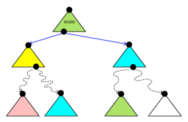
(e)	(f)

Figure 6. ARF construction in ESST.

4.8. Correctness of ESST

To prove the correctness of ESST, we need to introduce several notions and notations that relate the ESST algorithm with the operational semantics in Section 3. Given two states $s_{1}$ and $s_{2}$ whose domains are disjoint, we denote by $s_{1}\cup s_{2}$ the union of two states such that $\mathit{Dom}(s_{1}\cup s_{2})$ is $\mathit{Dom}(s_{1})\cup\mathit{Dom}(s_{2})$, and, for every $x\in\mathit{Dom}(s_{1}\cup s_{2})$, we have

$$(s_{1}\cup s_{2})(x)=\left\{\begin{array}[]{ll}s_{1}(x)&\mbox{if $x\in\mathit{Dom}(s_{1})$;}\\ s_{2}(x)&\mbox{otherwise.}\end{array}\right.$$

Let $P$ be a threaded program with $N$ threads, and $\gamma$ be a configuration

$$\langle(l_{1},s_{1}),\ldots,(l_{N},s_{N}),gs,\mathbb{S}\rangle,$$

of $P$. Let $\eta$ be an ARF node

$$(\langle l^{\prime}_{1},\varphi_{1}\rangle,\ldots,\langle l^{\prime}_{N},\varphi_{N}\rangle,\varphi,\mathbb{S}^{\prime}),$$

for $P$. We say that the configuration $\gamma$ satisfies the ARF node $\eta$, denoted by $\gamma\models\eta$ if and only if for all $i=1,\ldots,N$, we have $l_{i}=l^{\prime}_{i}$ and $s_{i}\cup gs\models\varphi_{i}$, $\bigcup_{i=1,\ldots,N}s_{i}\cup gs\models\varphi$, and $\mathbb{S}=\mathbb{S}^{\prime}$.

By the above definition, it is easy to see that, for any initial configuration $\gamma_{0}$ of $P$, we have $\gamma_{0}\models\eta_{0}$ for the initial ARF node $\eta_{0}$. In the sequel we refer to the configurations of $P$ and the ARF nodes (or connectors) for $P$ when we speak about configurations and ARF nodes (or connectors), respectively.

We now show that the node expansion rules E1 and E4 create successor nodes that are over-approximations of the configurations reachable by performing operations considered in the rules.

Lemma 1.

Let $\eta$ and $\eta^{\prime}$ be ARF nodes for a threaded program $P$ such that $\eta^{\prime}$ is a successor node of $\eta$. Let $\gamma$ be a configuration of $P$ such that $\gamma\models\eta$. The following properties hold:

1. If $\eta^{\prime}$ is obtained from $\eta$ by the rule E1 with the performed operation $op$, then, for any configuration $\gamma^{\prime}$ of $P$ such that $\gamma\stackrel{{\scriptstyle op}}{{\rightarrow}}\gamma^{\prime}$, we have $\gamma^{\prime}\models\eta^{\prime}$.

2. If $\eta^{\prime}$ is obtained from $\eta$ by the rule E4, then, for any configuration $\gamma^{\prime}$ of $P$ such that $\gamma\stackrel{{\scriptstyle\cdot}}{{\rightarrow}}\gamma^{\prime}$ and the scheduler states of $\eta^{\prime}$ and $\gamma^{\prime}$ coincide, we have $\gamma^{\prime}\models\eta^{\prime}$.

Let $\varepsilon$ be an ART edge with source node

$$\eta=(\langle l_{1},\varphi_{1}\rangle,\ldots,\langle l_{i},\varphi_{i}\rangle,\ldots\langle l_{N},\varphi_{N}\rangle,\varphi,\mathbb{S})$$

and target node

$$\eta^{\prime}=(\langle l_{1},\varphi^{\prime}_{1}\rangle,\ldots,\langle l^{\prime}_{i},\varphi^{\prime}_{i}\rangle,\ldots\langle l_{N},\varphi^{\prime}_{N}\rangle,\varphi^{\prime},\mathbb{S}^{\prime}),$$

such that $\mathbb{S}(s_{T_{i}})=\mathit{Running}$ and for all $j\neq i$, we have $\mathbb{S}(s_{T_{j}})\neq\mathit{Running}$. Let $G_{T_{i}}=(L,E,l_{0},L_{err})$ be the CFG for $T_{i}$ such that $(l_{i},op,l^{\prime}_{i})\in E$. Let $\gamma$ and $\gamma^{\prime}$ be configurations. We denote by $\gamma\stackrel{{\scriptstyle\varepsilon}}{{\rightarrow}}\gamma^{\prime}$ if $\gamma\models\eta$, $\gamma^{\prime}\models\eta^{\prime}$, and $\gamma\stackrel{{\scriptstyle op}}{{\rightarrow}}\gamma^{\prime}$. Note that, the operation $op$ is the operation labelling the edge of CFG, not the one labelling the ART edge $\varepsilon$. Similarly, we denote by $\gamma\stackrel{{\scriptstyle\kappa}}{{\rightarrow}}\gamma^{\prime}$ for an ARF connector $\kappa$ if $\gamma\models\eta$, $\gamma^{\prime}\models\eta^{\prime}$, and $\gamma\stackrel{{\scriptstyle\cdot}}{{\rightarrow}}\gamma^{\prime}$. Let $\hat{\rho}=\xi_{1},\ldots,\xi_{m}$ be an ARF path. That is, for each $i=1,\ldots,m$, the element $\xi_{i}$ is either an ART edge or an ARF connector. We denote by $\gamma\stackrel{{\scriptstyle\hat{\rho}}}{{\rightarrow}}\gamma^{\prime}$ if there exists a computation sequence $\gamma_{1},\ldots,\gamma_{m+1}$ such that $\gamma_{i}\stackrel{{\scriptstyle\xi_{i}}}{{\rightarrow}}\gamma_{i+1}$ for all $i=1,\ldots,m$, and $\gamma=\gamma_{1}$ and $\gamma^{\prime}=\gamma_{m+1}$.

In Section 3 the notion of strongest post-condition is defined as a set of reachable states after executing some operation. We now try to relate the notion of configuration with the notion of strongest post-condition. Let $\gamma$ be a configuration

$$\gamma=\langle(l_{1},s_{1}),\ldots,(l_{i},s_{i}),\ldots,(l_{N},s_{N}),gs,\mathbb{S}\rangle,$$

and $\varphi$ be a formula whose free variables range over $\bigcup_{k=1,\ldots,N}\mathit{Dom}(s_{k})\cup\mathit{Dom}(gs)$. We say that the configuration satisfies the formula $\varphi$, denoted by $\gamma\models\varphi$ if $\bigcup_{k=1,\ldots,N}s_{k}\cup gs\models\varphi$. Suppose that in the above configuration $\gamma$ we have $\mathbb{S}(s_{T_{i}})=\mathit{Running}$ and $\mathbb{S}(s_{T_{j}})\neq\mathit{Running}$ for all $j\neq i$. Let $G_{T_{i}}=(L,E,l_{0},L_{err})$ be the CFG for $T_{i}$ such that $(l_{i},op,l^{\prime}_{i})\in E$. Let $\hat{op}$ be $op$ if $op$ does not contain any primitive function call, otherwise $\hat{op}$ be $op^{\prime}$ as in the second case of the expansion rule E1. Then, for any configuration

$$\gamma^{\prime}=\langle(l_{1},s_{1}),\ldots,(l^{\prime}_{i},s^{\prime}_{i}),\ldots,(l_{N},s_{N}),gs^{\prime},\mathbb{S}^{\prime}\rangle,$$

such that $\gamma\stackrel{{\scriptstyle op}}{{\rightarrow}}\gamma^{\prime}$, we have $\gamma^{\prime}\models\mathit{SP}_{\hat{op}}(\varphi)$. Note that, the scheduler states $\mathbb{S}$ and $\mathbb{S}^{\prime}$ are not constrained by, respectively, $\varphi$ and $\mathit{SP}_{\hat{op}}(\varphi)$, and so they can be different.

When $\textsc{ESST}(P)$ terminates and reports that $P$ is safe, we require that, for every configuration $\gamma$ reachable in $P$, there is a node in $\mathcal{F}$ such that the configuration satisfies the node. We denote by $\mathit{Reach}(P)$ the set of configurations reachable in $P$, and by $\mathit{Nodes}(\mathcal{F})$ the set of nodes in $\mathcal{F}$.

Theorem 2 (Correctness).

Let $P$ be a threaded program. For every terminating execution of $\textsc{ESST}(P)$, we have the following properties:

1. If $\textsc{ESST}(P)$ returns a feasible counter-example path $\hat{\rho}$, then we have $\gamma\stackrel{{\scriptstyle\hat{\rho}}}{{\rightarrow}}\gamma^{\prime}$ for an initial configuration $\gamma$ and an error configuration $\gamma^{\prime}$ of $P$.

2. If $\textsc{ESST}(P)$ returns a safe ARF $\mathcal{F}$, then for every configuration $\gamma\in\mathit{Reach}(P)$, there is an ARF node $\eta\in\mathit{Nodes}(\mathcal{F})$ such that $\gamma\models\eta$.

5. ESST + Partial-Order Reduction

The ESST algorithm often has to explore a large number of possible thread interleavings. However, some of them might be redundant because the order of interleavings of some threads is irrelevant. Given $N$ threads such that each of them accesses a disjoint set of variables, there are $N!$ possible interleavings that ESST has to explore. The constructed ARF will consists of $2^{N}$ abstract states (or nodes). Unfortunately, the more abstract states to explore, the more computations of abstract strongest post-conditions are needed, and the more coverage checks are involved. Moreover, the more interleavings to explore, the more possible spurious counter-example paths to rule out, and thus the more refinements are needed. As refinements result in keeping track of additional predicates, the computations of abstract strongest post-conditions become expensive. Consequently, exploring all possible interleavings degrades the performance of ESST and leads to state explosion.

Partial-order reduction techniques (POR) [God96, Pel93, Val91] have been successfully applied in explicit-state software model checkers like SPIN [Hol05] and VeriSoft [God05] to avoid exploring redundant interleavings. POR has also been applied to symbolic model checking techniques as shown in [KGS06, WYKG08, ABH⁺01]. In this section we will extend the ESST algorithm with POR techniques. However, as we will see, such an integration is not trivial because we need to ensure that in the construction of the ARF the POR techniques do not make ESST unsound.

5.1. Partial-Order Reduction (POR)

Partial-order reduction (POR) is a model checking technique that is aimed at combating the state explosion by exploring only representative subset of all possible interleavings. POR exploits the commutativity of concurrent transitions that result in the same state when they are executed in different orders.

We present POR using the standard notions and notations used in [God96, CGP99]. We model a concurrent program as a transition system $M=(S,S_{0},T)$, where $S$ is the finite set of states, $S_{0}\subset S$ is the set of initial states, and $T$ is a set of transitions such that for each $\alpha\in T$, we have $\alpha\subset S\times S$. We say that $\alpha(s,s^{\prime})$ holds and often write it as $s\stackrel{{\scriptstyle\alpha}}{{\rightarrow}}s^{\prime}$ if $(s,s^{\prime})\in\alpha$. A state $s^{\prime}$ is a successor of a state $s$ if $s\stackrel{{\scriptstyle\alpha}}{{\rightarrow}}s^{\prime}$ for some transition $\alpha\in T$. In the following we will only consider deterministic transitions, and often write $s^{\prime}=\alpha(s)$ for $\alpha(s,s^{\prime})$. A transition $\alpha$ is enabled in a state $s$ if there is a state $s^{\prime}$ such that $\alpha(s,s^{\prime})$ holds. The set of transitions enabled in a state $s$ is denoted by $\mathit{enabled}(s)$. A path from a state $s$ in a transition system is a finite or infinite sequence $s_{0}\stackrel{{\scriptstyle\alpha_{0}}}{{\rightarrow}}s_{1}\stackrel{{\scriptstyle\alpha_{1}}}{{\rightarrow}}\cdots$ such that $s=s_{0}$ and $s_{i}\stackrel{{\scriptstyle\alpha_{i}}}{{\rightarrow}}s_{i+1}$ for all $i$. A path is empty if the sequence consists only of a single state. The length of a finite path is the number of transitions in the path.

Let $M=(S,S_{0},T)$ be a transition system, we denote by $\mathit{Reach}(S_{0},T)\subseteq S$ the set of states reachable from the states in $S_{0}$ by the transitions in $T$: for a state $s\in\mathit{Reach}(S_{0},T)$, there is a finite path $s_{0}\stackrel{{\scriptstyle\alpha_{0}}}{{\rightarrow}}\ldots\stackrel{{\scriptstyle\alpha_{n-1}}}{{\rightarrow}}s_{n}$ system such that $s_{0}\in S_{0}$ and $s=s_{n}$. In this work we are interested in verifying safety properties in the form of program assertion. To this end, we assume that there is a set $\mathit{T_{err}}\subseteq T$ of error transitions such that the set

$$\mathit{E}_{M,\mathit{T_{err}}}=\{s\in S\mid\exists s^{\prime}\in S.\exists\alpha\in\mathit{T_{err}}.\ \ \alpha(s^{\prime},s)\mbox{ holds }\}$$

is the set of error states of $M$ with respect to $\mathit{T_{err}}$. A transition system $M=(S,S_{0},T)$ is safe with respect to the set $\mathit{T_{err}}\subseteq T$ of error transitions iff $\mathit{Reach}(S_{0},T)\cap\mathit{E}_{M,\mathit{T_{err}}}=\emptyset$.

Selective search in POR exploits the commutativity of concurrent transitions. The concept of commutativity of concurrent transitions can be formulated by defining an independence relation on pairs of transitions.

[Independence Relation, Independent Transitions] An independence relation $I\subseteq T\times T$ is a symmetric, anti-reflexive relation such that for each state $s\in S$ and for each $(\alpha,\beta)\in I$ the following conditions are satisfied:

Enabledness: If $\alpha$ is in $\mathit{enabled}(s)$, then $\beta$ is in $\mathit{enabled}(s)$ iff $\beta$ is in $\mathit{enabled}(\alpha(s))$.

Commutativity: If $\alpha$ and $\beta$ are in $\mathit{enabled}(s)$, then $\alpha(\beta(s))=\beta(\alpha(s))$. We say that two transitions $\alpha$ and $\beta$ are independent of each other if for every state $s$ they satisfy the enabledness and commutativity conditions. We also say that two transitions $\alpha$ and $\beta$ are independent in a state $s$ of each other if they satisfy the enabledness and commutativity conditions in $s$.

In the sequel we will use the notion of valid dependence relation to select a representative subset of transitions that need to be explored.

[Valid Dependence Relation] A valid dependence relation $D\subseteq T\times T$ is a symmetric, reflexive relation such that for every $(\alpha,\beta)\not\in D$, the transitions $\alpha$ and $\beta$ are independent of each other.

5.1.1. The Persistent Set Approach

To reduce the number of possible interleavings, in every state visited during the state space exploration one only explores a representative subset of transitions that are enabled in that state. However, to select such a subset we have to avoid possible dependencies that can happen in the future. To this end, we appeal to the notion of persistent set [God96].

[Persistent Set] A set $P\subseteq T$ of enabled transitions in a state $s$ is persistent in $s$ if for every finite non-empty path $s=s_{0}\stackrel{{\scriptstyle\alpha_{0}}}{{\rightarrow}}s_{1}\stackrel{{\scriptstyle\alpha_{1}}}{{\rightarrow}}\cdots\stackrel{{\scriptstyle\alpha_{n-1}}}{{\rightarrow}}s_{n}\stackrel{{\scriptstyle\alpha_{n}}}{{\rightarrow}}s_{n+1}$ such that $\alpha_{i}\not\in P$ for all $i=0,\ldots,n$, we have $\alpha_{n}$ independent of any transition in $P$ in $s_{n}$.

Note that the persistent set in a state is not unique. To guarantee the existence of successor state, we impose the successor-state condition on the persistent set: the persistent set in $s$ is empty iff so is $\mathit{enabled}(s)$. In the sequel we assume persistent sets satisfy the successor-state condition. We say that a state $s$ is fully expanded if the persistent set in $s$ equals $\mathit{enabled}(s)$. It is easy to see that, for any transition $\alpha$ not in the persistent set $P$ in a state $s$, the transition $\alpha$ is disabled in $s$ or independent of any transition in $P$.

We denote by $\mathit{Reach}_{red}(S_{0},T)\subseteq S$ the set of states reachable from the states in $S_{0}$ by the transitions in $T$ such that, during the state space exploration, in every visited state we only explore the transitions in the persistent set in that state. That is, for a state $s\in\mathit{Reach}_{red}(S_{0},T)$, there is a finite path $s_{0}\stackrel{{\scriptstyle\alpha_{0}}}{{\rightarrow}}\ldots\stackrel{{\scriptstyle\alpha_{n-1}}}{{\rightarrow}}s_{n}$ in the transition system such that $s_{0}\in S_{0}$ and $s=s_{n}$, and $\alpha_{i}$ is in the persistent set of $s_{i}$, for $i=0,\ldots,n-1$. It is easy to see that $\mathit{Reach}_{red}(S_{0},T)\subseteq\mathit{Reach}(S_{0},T)$.

To preserve safety properties of a transition system, we need to guarantee that the reduction by means of persistent sets does not remove all interleavings that lead to an error state. To this end, we impose the cycle condition on $\mathit{Reach}_{red}(S_{0},T)$ [CGP99, Pel93]: a cycle is not allowed if it contains a state in which a transition $\alpha$ is enabled, but $\alpha$ is never included in the persistent set of any state $s$ on the cycle. That is, if there is a cycle $s_{0}\stackrel{{\scriptstyle\alpha_{0}}}{{\rightarrow}}\ldots\stackrel{{\scriptstyle\alpha_{n-1}}}{{\rightarrow}}s_{n}=s_{0}$ induced by the states $s_{0},\ldots,s_{n-1}$ in $\mathit{Reach}_{red}(S_{0},T)$ such that $\alpha_{i}$ is persistent in $s_{i}$, for $i=0,\ldots,n-1$ and $\alpha\in\mathit{enabled}(s_{j})$ for some $0\leq j<n$, then $\alpha$ must be in the persistent set of any of $s_{0},\ldots,s_{n-1}$.

Theorem 3.

A transition system $M=(S,S_{0},T)$ is safe w.r.t. a set $\mathit{T_{err}}\subseteq T$ of error transitions iff $\mathit{Reach}_{red}(S_{0},T)$ that satisfies the cycle condition does not contain any error state from $\mathit{E}_{M,\mathit{T_{err}}}$.

5.1.2. The Sleep Set Approach

The sleep set POR technique exploits independencies of enabled transitions in the current state. For example, suppose that in some state $s$ there are two enabled transitions $\alpha$ and $\beta$, and they are independent of each other. Suppose further that the search explores $\alpha$ first from $s$. Then, when the search explores $\beta$ from $s$ such that $s\stackrel{{\scriptstyle\beta}}{{\rightarrow}}s^{\prime}$ for some state $s^{\prime}$, we associate with $s^{\prime}$ a sleep set containing only $\alpha$. From $s^{\prime}$ the search only explores transitions that are not in the sleep set of $s^{\prime}$. That is, although the transition $\alpha$ is still enabled in $s^{\prime}$, it will not be explored. Both persistent set and sleep set techniques are orthogonal and complementary, and thus can be applied simultaneously. Note that the sleep set technique only removes transitions, and not states. Thus, Theorem 3 still holds when the sleep set technique is applied.

5.2. Applying POR to ESST

The key idea of applying POR to ESST is to select a representative subset of scheduler states output by the scheduler in ESST. That is, instead of creating successor nodes with all scheduler states from $\{\mathbb{S}_{1},\ldots,\mathbb{S}_{n}\}=\textsc{Sched}(\mathbb{S})$, for some state $\mathbb{S}$, we create successor nodes with the representative subset of $\{\mathbb{S}_{1},\ldots,\mathbb{S}_{n}\}$. However, such an application is non-trivial. The ESST algorithm is based on the construction of an ARF that describes the reachable abstract states, while the exposition of POR before is based on the analysis of reachable concrete states. As we will see later, some POR properties that hold in the concrete state space do not hold in the abstract state space. Nevertheless, in applying POR to ESST one needs to guarantee that the original ARF is safe if and only if the reduced ARF, obtained by the restriction on the scheduler’s output, is safe. In particular, the construction of reduced ARF has to check if the cycle condition is satisfied in its concretization.

To integrate POR techniques into the ESST algorithm, we first need to identify fragments in the threaded program that count as transitions in the transition system. In the previous description of POR the execution of a transition is atomic, that is, its execution cannot be interleaved by the executions of other transitions. We introduce the notion of atomic block as the notion of transition in the threaded program. Intuitively, an atomic block is a block of operations between calls to primitive functions that can suspend the thread. Let us call such primitive functions blocking functions.

An atomic block of a thread is a rooted subgraph of the CFG such that the subgraph satisfies the following conditions:

1. its unique entry is the entry of the CFG or the location that immediately follows a call to a blocking function;

2. its exit is the exit of the CFG or the location that immediately follows a call to a blocking function; and

3. there is no call to a blocking function in any CFG path from the entry to an exit except the one that precedes the exit.

Note that an atomic block has a unique entry, but can have multiple exits. We often identify an atomic block by its entry. Furthermore, we denote by $\mathit{ABlock}$ the set of atomic blocks.

Consider a thread whose CFG is depicted in Figure 7(a). Let wait($\ldots$) be the only call to a blocking function in the CFG. Figures 7(b) and (c) depicts the atomic blocks of the thread. The atomic block in Figure 7(b) starts from $l_{0}$ and exits at $l_{5}$ and $l_{7}$, while the one in Figure 7(c) starts from $l_{5}$ and exits at $l_{5}$ and $l_{7}$.

(a)	(b)	(c)

Figure 7. Identifying atomic blocks.

Note that, an atomic block can span over multiple basic blocks or even multiple large blocks in the basic block or large block encoding [BCG⁺09]. In the sequel we will use the terms transition and atomic block interchangeably.

Prior to computing persistent sets, we need to compute valid dependence relations. The criteria for two transitions being dependent are different from one application domain to the other. Cooperative threads in many embedded system domains employ event-based synchronizations through event waits and notifications. Different domains can have different types of event notification. For generality, we anticipate two kinds of notification: immediate and delayed notifications. An immediate notification is materialized immediately at the current time or at the current cycle (for cycle-based semantics). Threads that are waiting for the notified events are made runnable upon the notification. A delayed notification is scheduled to be materialized at some future time or at the end of the current cycle. In some domains delayed notifications can be cancelled before they are triggered.

For example, in a system design language that supports event-based synchronization, a pair $(\alpha,\beta)$ of atomic blocks are in a valid dependence relation if one of the following criteria is satisfied: (1) the atomic block $\alpha$ contains a write to a shared (or global) variable $g$, and the atomic block $\beta$ contains a write or a read to $g$; (2) the atomic block $\alpha$ contains an immediate notification of an event $e$, and the atomic block $\beta$ contains a wait for $e$; (3) the atomic block $\alpha$ contains a delayed notification of an event $e$, and the atomic block $\beta$ contains a cancellation of a notification of $e$. Note that the first criterion is a standard criterion for two blocks to become dependent on each other. That is, the order of executions of the two blocks is relevant because different orders yield different values assigned to variables. The second and the third criteria are specific to event-based synchronization language. An event notification can make runnable a thread that is waiting for a notification of the event. A waiting thread misses an event notification if the thread waited for such a notification after another thread had made the notification. Thus, the order of executions of atomic blocks containing event waits and event notifications is relevant. Similarly for the delayed notification in the third criterion. Given criteria for being dependent, one can use static analysis techniques to compute a valid dependence relation.

Algorithm 1 Persistent sets.

Input: a set $B_{en}$ of enabled atomic blocks.

Output: a persistent set $P$.

(1) Let $B:=\{\alpha\}$, where $\alpha\in B_{en}$. (2) For each atomic block $\alpha\in B$: (a) If $\alpha\in B_{en}$ ($\alpha$ is enabled): $\bullet$ (b) Add into $B$ every atomic block $\beta$ such that $(\alpha,\beta)\in D$. (c) If $\alpha\not\in B_{en}$ ($\alpha$ is disabled): $\bullet$ (d) Add into $B$ a necessary enabling set for $\alpha$ with $B_{en}$. (3) Repeat step 2 until no more atomic blocks can be added into $B$. (4) $P:=B\cap B_{en}$.

To have small persistent sets, we need to know whether a disabled transition that has a dependence relation with the currently enabled ones can be made enabled in the future. To this end, we use the notion of necessary enabling set introduced in [God96].

[Necessary Enabling Set] Let $M=(S,S_{0},T)$ be a transition system such that a transition $\alpha\in T$ is diabled in a state $s\in S$. A set $T_{\alpha,s}\subseteq T$ is a necessary enabling set for $\alpha$ in $s$ if for every finite path $s=s_{0}\stackrel{{\scriptstyle\alpha_{0}}}{{\rightarrow}}\cdots\stackrel{{\scriptstyle\alpha_{n-1}}}{{\rightarrow}}s_{n}$ in $M$ such that $\alpha$ is disabled in $s_{i}$, for all $0\leq i<n$, but is enabled in $s_{n}$, a transition $t_{j}$, for some $0\leq j\leq n-1$, is in $T_{\alpha,s}$. A set $T_{\alpha,T_{en}}\subseteq T$, for $T_{en}\subseteq T$, is a necessary enabling set for $\alpha$ with $T_{en}$ if $T_{\alpha,T_{en}}$ is a necessary enabling set for $\alpha$ in every state $s$ such that $T_{en}$ is the set of enabled transitions in $s$.

Intuitively, a necessary enabling set $T_{\alpha,s}$ for a transition $\alpha$ in a state $s$ is a set of transitions such that $\alpha$ cannot become enabled in the future before at least a transition in $T_{\alpha,s}$ is executed.

Algorithm 1 computes persistent sets using a valid dependence relation $D$. It is easy to see that the persistent set computed by the algorithm satisfies the successor-state condition. The algorithm is also a variant of the stubborn set algorithm presented in [God96], that is, we use a valid dependence relation as the interference relation used in the latter algorithm.

We apply POR to the ESST algorithm by modifying the ARF node expansion rule E4, described in Section 4 in two steps. First we compute a persistent set from a set of scheduler states output by the function Sched. Second, we ensure that the cycle condition is satisfied by the concretization of the constructed ARF.

We introduce the function Persistent that computes a persistent set of a set of scheduler states. Persistent takes as inputs an ARF node and a set $\mathcal{S}$ of scheduler states, and outputs a subset $\mathcal{S}^{\prime}$ of $\mathcal{S}$. The input ARF node keeps track of the thread locations, which are used to identify atomic blocks, while the input scheduler states keep track of the status of the threads. From the ARF node and the set $\mathcal{S}$, the function Persistent extracts the set $B_{en}$ of enabled atomic blocks. Persistent then computes a persistent set $P$ from $B_{en}$ using Algorithm 1. Finally, Persistent constructs back a subset $\mathcal{S}^{\prime}$ of the input set $\mathcal{S}$ of scheduler states from the persistent set $P$.

Let $\eta=(\langle l_{1},\varphi_{1}\rangle,\ldots,\langle l_{N},\varphi_{N}\rangle,\varphi,\mathbb{S})$ be an ARF node that is going to be expanded. We replace the rule E4 in the following way: instead of creating a new ART for each state $\mathbb{S}^{\prime}\in\textsc{Sched}(\mathbb{S})$, we create a new ART whose root is the node $(\langle l_{1},\varphi_{1}\rangle,\ldots,\langle l_{N},\varphi_{N}\rangle,\varphi,\mathbb{S}^{\prime})$ for each state $\mathbb{S}^{\prime}\in\textsc{Persistent}(\eta,\textsc{Sched}(\mathbb{S}))$ (rule E4’).

To guarantee the preservation of safety properties, we have to check that the cycle condition is satisfied. Following [CGP99], we check a stronger condition: at least one state along the cycle is fully expanded. In the ESST algorithm a potential cycle occurs if an ARF node is covered by one of its predecessors in the ARF. Let $\eta=(\langle l_{1},\varphi_{1}\rangle,\ldots,\langle l_{N},\varphi_{N}\rangle,\varphi,\mathbb{S})$ be an ARF node. We say that the scheduler state $\mathbb{S}$ is running if there is a running thread in $\mathbb{S}$. We also say that the node $\eta$ is running if its scheduler state $\mathbb{S}$ is. Note that during ARF expansion the input of Sched is always a non-running scheduler state. A path in an ARF can be represented as a sequence $\eta_{0},\ldots,\eta_{m}$ of ARF nodes such that for all $i$, we have $\eta_{i+1}$ is a successor of $\eta_{i}$ in the same ART or there is an ARF connector from $\eta_{i}$ to $\eta_{i+1}$. Given an ARF node $\eta$ of ARF $\mathcal{F}$, we denote by $\mathit{ARFPath}(\eta,\mathcal{F})$ the ARF path $\eta_{0},\ldots,\eta_{m}$ such that $\eta_{0}$ has neither a predecessor ARF node nor an incoming ARF connector, and $\eta_{m}=\eta$. Let $\hat{\rho}$ be an ARF path, we denote by $\mathit{NonRunning}(\hat{\rho})$ the maximal subsequence of non-running node in $\hat{\rho}$.

Algorithm 2 ARF expansion algorithm for non-running node.

Input: a non-running ARF node $\eta$ that contains no error locations.

(1) Let $\mathit{NonRunning}(\mathit{ARFPath}(\eta,\mathcal{F}))$ be $\eta_{0},\ldots,\eta_{m}$ such that $\eta=\eta_{m}$ (2) If there exists $i<m$ such that $\eta_{i}$ covers $\eta$: (a) Let $\eta_{m-1}=(\langle l^{\prime}_{1},\varphi^{\prime}_{1}\rangle,\ldots,\langle l^{\prime}_{N},\varphi^{\prime}_{N}\rangle,\varphi^{\prime},\mathbb{S}^{\prime})$. (b) If $\textsc{Persistent}(\eta_{m-1},\textsc{Sched}(\mathbb{S}^{\prime}))\subset\textsc{Sched}(\mathbb{S}^{\prime})$: $\bullet$ (c) For all $\mathbb{S}^{\prime\prime}\in\textsc{Sched}(\mathbb{S}^{\prime})\setminus\textsc{Persistent}(\eta_{m-1},\textsc{Sched}(\mathbb{S}^{\prime}))$: $-$ (d) Create a new ART with root node $(\langle l^{\prime}_{1},\varphi^{\prime}_{1}\rangle,\ldots,\langle l^{\prime}_{N},\varphi^{\prime}_{N}\rangle,\varphi^{\prime},\mathbb{S}^{\prime\prime})$. (3) If $\eta$ is covered: Mark $\eta$ as covered. (4) If $\eta$ is not covered: Expand $\eta$ by rule E4’.

Algorithm 2 shows how a non-running ARF node $\eta$ is expanded in the presence of POR. We assume that $\eta$ is not an error node. The algorithm fully expands the immediate non-running predecessor node of $\eta$ when a potential cycle is detected. Otherwise the node is expanded as usual.

Our POR technique slightly differs from that of [CGP99]. On computing the successor states of a state $s$, the technique in [CGP99] tries to compute a persistent set $P$ in $s$ that does not create a cycle. That is, particularly for the depth-first search (DFS) exploration, for every $\alpha$ in $P$, the successor state $\alpha(s)$ is not in the DFS stack. If it does not succeed, then it fully expands the state. Because the technique in [CGP99] is applied to the explicit-state model checking, computing the successor state $\alpha(s)$ is cheap.

In our context, to detect a cycle, one has to expand an ARF node by a transition (or an atomic block) that can span over multiple operations in the CFG, and thus may require multiple applications of the rule E1. As the rule involves expensive computations of abstract strongest post-conditions, detecting a cycle using the technique in [CGP99] is bound to be expensive.

In addition to coverage check, in the above algorithm one can also check if the detected cycle is spurious. We only fully expand a node iff the detected cycle is not spurious. When cycles are rare, the benefit of POR can be defeated by the price of generating and solving the constraints representing the cycle.

POR based on sleep sets can also be applied to ESST. First, we extend the node of ARF to include a sleep set. That is, an ARF node is a tuple $(\langle l_{1},\varphi_{1}\rangle,\ldots,\langle l_{N},\varphi_{N}\rangle,\varphi,\mathbb{S},Z)$, where the sleep set $Z$ is a set of atomic blocks. The sleep set is ignored during coverage check. Second, from the set of enabled atomic blocks and the sleep set of the current node, we compute a subset of enabled atomic blocks and a mapping from every atomic block in the former subset to a successor sleep set.

Let $D$ be a valid dependence relation, Algorithm 3 shows how to compute a reduced set of enabled transitions $B_{red}$ and a mapping $M_{Z}$ to successor sleep sets using $D$. The input of the algorithm is a set $B_{en}$ of enabled atomic blocks and the sleep set $Z$ of the current node. Note that the set $B_{en}$ can be a persistent set obtained by Algorithm 1.

Algorithm 3 Sleep sets.

Input:

• a set $B_{en}$ of enabled atomic blocks. • a sleep set $Z$.

Output:

• a reduced set $B_{red}\subseteq B_{en}$ of enabled atomic blocks. • a mapping $M_{Z}:B_{red}\rightarrow\mathcal{P}(\mathit{ABlock})$

(1) $B_{red}:=B_{en}\setminus Z$. (2) For all $\alpha\in B_{red}$: (a) For all $\beta\in Z$: $\bullet$ (b) If $(\alpha,\beta)\not\in D$ ($\alpha$ and $\beta$ are independent): $M_{Z}[\alpha]:=M_{Z}[\alpha]\cup\{\beta\}$. (c) $Z:=Z\cup\{\alpha\}$.

Similar to the persistent set technique, we introduce the function Sleep that takes as inputs an ARF node $\eta$ and a set of scheduler states $\mathcal{S}$, and outputs a subset $\mathcal{S}^{\prime}$ of $\mathcal{S}$ along with the above mapping $M_{Z}$. From the ARF node and the scheduler states, Sleep extracts the set $B_{en}$ of enabled atomic blocks and the current sleep set. Sleep then computes a subset $B_{red}$ of $B_{en}$ of enabled atomic blocks and the mapping $M_{Z}$ using Algorithm 3. Finally, Sleep constructs back a subset $\mathcal{S}^{\prime}$ of the input set $\mathcal{S}$ of scheduler states from the set $B_{red}$ of enabled atomic blocks.

Let $\eta=(\langle l_{1},\varphi_{1}\rangle,\ldots,\langle l_{N},\varphi_{N}\rangle,\varphi,\mathbb{S},Z)$ be an ARF node that is going to be expanded. We replace the rule E4 in the following way: let $(\mathcal{S}^{\prime},M_{Z})=\textsc{Sleep}(\eta,\textsc{Sched}(\mathbb{S}))$, create a new ART whose root is the node $(\langle l_{1},\varphi_{1}\rangle,\ldots,\langle l_{N},\varphi_{N}\rangle,\varphi,\mathbb{S}^{\prime},M_{Z}[l^{\prime}])$ for each $\mathbb{S}^{\prime}\in\mathcal{S}^{\prime}$ such that $l^{\prime}$ is the atomic block of the running thread in $\mathbb{S}^{\prime}$ (rule E4”).

One can easily combine persistent and sleep sets by replacing the above computation $(\mathcal{S}^{\prime},M_{Z})=\textsc{Sleep}(\eta,\textsc{Sched}(\mathbb{S}))$ by $(\mathcal{S}^{\prime},M_{Z})=\textsc{Sleep}(\eta,\textsc{Persistent}(\eta,\textsc{Sched}(\mathbb{S})))$.

5.3. Correctness of ESST + POR

The correctness of POR with respect to verifying program assertions in transition systems has been shown in Theorem 3. The correctness proof relies on the enabledness and commutativity of independent transitions. However, the proof is applied in the concrete state space of the transition system, while the ESST algorithm works in the abstract state space represented by the ARF. The following observation shows that two transitions that are independent in the concrete state space may not commute in the abstract state space.

Figure 8. Independent transitions
do not commute in
abstract state space.

For simplicity of presentation, we represent an abstract state by a formula representing a region. Let $g_{1},g_{2}$ be global variables, and $p,q$ be predicates such that $p\Leftrightarrow(g_{1}<g_{2})$ and $q\Leftrightarrow(g1=g2)$. Let $\alpha$ be the transition $g_{1}$ := $g_{1}$ - 1 and $\beta$ be the transition $g_{2}$ := $g_{2}$ - 1. It is obvious that $\alpha$ and $\beta$ are independent of each other. However, Figure 8 shows that the two transitions do no commute when we start from an abstract state $\eta_{1}$ such that $\eta_{1}\Leftrightarrow p$. The edges in the figure represent the computation of abstract strongest post-condition of the corresponding abstract states and transitions.

Even though two independent transitions do not commute in the abstract state space, they still commute in the concrete state space overapproximated by the abstract state space, as shown by the lemma below.

Lemma 4.

Let $\alpha$ and $\beta$ be transitions that are independent of each other such that for concrete states $s_{1},s_{2},s_{3}$ and abstract state $\eta$ we have $s_{1}\models\eta$, and both $\alpha(s_{1},s_{2})$ and $\beta(s_{2},s_{3})$ hold. Let $\eta^{\prime}$ be the abstract successor state of $\eta$ by applying the abstract strongest post-operator to $\eta$ and $\beta$, and $\eta^{\prime\prime}$ be the abstract successor state of $\eta^{\prime}$ by applying the abstract strongest post-operator to $\eta^{\prime}$ and $\alpha$. Then, there are concrete states $s_{4}$ and $s_{5}$ such that: $\beta(s_{1},s_{4})$ holds, $s_{4}\models\eta^{\prime}$, $\beta(s_{4},s_{5})$ holds, $s_{5}\models\eta^{\prime\prime}$, and $s_{3}=s_{5}$.

The above lemma shows that POR can be applied in the abstract state space. Let $\textsc{ESST}_{\textsc{POR}}$ be the ESST algorithm with POR. The correctness of POR in ESST is stated by the following theorem:

Theorem 5.

Let $P$ be a threaded sequential program. For every terminating executions of $\textsc{ESST}(P)$ and $\textsc{ESST}_{\textsc{POR}}(P)$, we have that $\textsc{ESST}(P)$ reports safe iff so does $\textsc{ESST}_{\textsc{POR}}(P)$.

6. Experimental Evaluation

In this section we show an experimental evaluation of the ESST algorithm in the verification of multi-threaded programs in the FairThreads [Bou06] programming framework. The aim of this evaluation is to show the effectiveness of ESST and of the partial-order reduction applied to ESST. By following the same methodology, the ESST algorithm can be adapted to other programming frameworks, like SpecC [GDPG01] and OSEK/VDX [OSE05], with moderate effort.

6.1. Verifying FairThreads

FairThreads is a framework for programming multi-threaded software that allows for mixing both cooperative and preemptive threads. As we want to apply ESST, we only deal with the cooperative threads. FairThreads includes a scheduler that executes threads according to a simple round-robin policy. FairThreads also provides a programming interface that allows threads to synchronize and communicate with each others. Examples of synchronization primitives of FairThreads are as follows: await($e$) for waiting for the notification of event $e$ if such a notification does not exist, generate($e$) for generating a notification of event $e$, cooperate for yielding the control back to the scheduler, and join($t$) for waiting for the termination of thread $t$.

The scheduler of FairThreads is shown in Figure 9. At the beginning all threads are set to be runnable. The executions of threads consist of a series of instants in which the scheduler runs all runnable threads, in a deterministic round-robin fashion, until there are no more runnable threads.

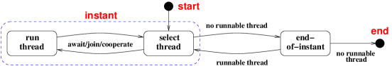
Figure 9. The scheduler of FairThreads.

A running thread can yield the control back to the scheduler either by waiting for an event notification (await), by cooperating (cooperate), or by waiting for another thread to terminate (join). A thread that executes the primitive await($e$) can observe the notification of $e$ even though the notification occurs long before the execution of the primitive, so long as the execution of await($e$) is still in the same instant of the notification of $e$. Thus, the execution of await does not necessarily yields the control back to the scheduler.

When there are no more runnable threads, the scheduler enters the end-of-instant phase. In this phase the scheduler wakes up all threads that had cooperated during the last instant, and also clears all event notifications. The scheduler then starts a new instant if there are runnable threads; otherwise the execution ends.

The operational semantics of cooperative FairThreads has been described in [Bou02]. However, it is not clear from the semantics whether the round-robin order of the thread executions remains the same from one instant to the other. Here, we assume that the order is the same from one instant to the other. The operational semantics does not specify either the initial round-robin order of the thread executions. Thus, for the verification, one needs to explore all possible round-robin orders. This situation could easily degrade the performance of ESST and possibly lead to state explosion. The POR techniques described in Section 5 could in principle address this problem.

In this section we evaluate two software model checking approaches for the verification of FairThreads programs. In the first approach we rely on a translation from FairThreads into sequential programs (or sequentialization), such that the resulting sequential programs contain both the mapping of the cooperative threads in the form of functions and the encoding of the FairThreads scheduler. The thread activations are encoded as function calls from the scheduler function to the functions that correspond to the threads. The program can be thought of as jumping back and forth between the “control level” imposed by the scheduler, and the “logical level” implemented by the threads. Having the sequential program, we then use off-the-shelf software model checkers to verify the programs.

In the second approach we apply the ESST algorithm to verify FairThreads programs. In this approach we define a set of primitive functions that implement FairThreads synchronization functions, and instantiate the scheduler of ESST with the FairThreads scheduler. We then translate the FairThreads program into a threaded program such that there is a one-to-one correspondence between the threads in the FairThreads program and in the resulting threaded program. Furthermore, each call to a FairThreads synchronization function is translated into a call to the corresponding primitive function. The ESST algorithm is then applied to the resulting threaded program.

6.2. Experimental evaluation setup

The ESST algorithm has been implemented in the Kratos software model checker [CGM⁺11]. In this work we have extended Kratos with the FairThreads scheduler and the primitive functions that correspond to the FairThreads synchronization functions.

We have carried out a significant experimental evaluation on a set of benchmarks taken and adapted from the literature on verification of cooperative threads. For example, the fact* benchmarks are extracted from [JBGT10], which describes a synchronous approach to verifying the absence of deadlocks in FairThreads programs. We adapted the benchmarks by recoding the bad synchronization, that can cause deadlocks, as an unreachable false assertion. The gear-box benchmark is taken from the case study in [WH08]. This case study is about an automated gearbox control system that consists of a five-speed gearbox and a dry clutch. Our adaptation of this benchmark does not model the timing behavior of the components and gives the same priority to all tasks (or threads) of the control system. In our case we considered the verification of safety properties that do not depend on the timing behavior. Ignoring the timing behavior in this case results in more non-determinism than that of the original case study. The ft-pc-sfifo* and ft-token-ring* benchmarks are taken and adapted from, respectively, the pc-sfifo* and token-ring* benchmarks used in [CMNR10, CNR11]. All considered benchmarks satisfy the restriction of ESST: the arguments passed to every call to a primitive function are constants.

For the sequentialized version of FairThreads programs, we experimented with several state-of-the-art predicate-abstraction based software model checkers, including SatAbs-3.0 [CKSY05], CpaChecker [BK11], and the sequential analysis of Kratos [CGM⁺11]. We also experimented with CBMC-4.0 [CKL04] for bug hunting with bounded model checking (BMC) [BCCZ99]. For the BMC experiment, we set the size of loop unwindings to 5 and consider only the unsafe benchmarks. All benchmarks and tools’ setup are available at http://es.fbk.eu/people/roveri/tests/jlmcs-esst.

We ran the experiments on a Linux machine with Intel-Xeon DC 3GHz processor and 4GB of RAM. We fixed the time limit to 1000 seconds, and the memory limit to 4GB.

6.3. Results of Experiments

The results of experiments are shown in Table 1, for the run times, and in Table 2, for the numbers of explored abstract states by ESST. The column V indicates the status of the benchmarks: S for safe and U for unsafe. In the experiments we also enable the POR techniques in ESST. The column No-POR indicates that during the experiments POR is not enabled. The column P-POR indicates that only the persistent set technique is enabled, while the column S-POR indicates that only the sleep set technique is enabled. The column PS-POR indicates that both the persistent set and the sleep set techniques are enabled. We mark the best results with bold letters, and denote the out-of-time results by T.O.

The results clearly show that ESST outperforms the predicate abstraction based sequentialization approach. The main bottleneck in the latter approach is the number of predicates that the model checkers need to keep track of to model details of the scheduler. For example, on the ft-pc-sfifo1.c benchmark SatAbs, CpaChecker, and the sequential analysis of Kratos needs to keep track of, respectively, 71, 37, and 45 predicates. On the other hand, ESST only needs to keep track of 8 predicates on the same benchmark.

Regarding the refinement steps, ESST needs less abstraction-refinement iterations than other techniques. For example, starting with the empty precision, the sequential analysis of Kratos needs 8 abstraction-refinement iterations to verify fact2, and 35 abstraction-refinement iterations to verify ft-pc-sfifo1. ESST, on the other hand, verifies fact2 without performing any refinements at all, and verifies ft-pc-sfifo1 with only 3 abstraction-refinement iterations.

The BMC approach, represented by CBMC, is ineffective on our benchmarks. First, the breadth-first nature of the BMC approach creates big formulas on which the satisfiability problems are hard. In particular, CBMC employs bit-precise semantics, which contributes to the hardness of the problems. Second, for our benchmarks, it is not feasible to identify the size of loop unwindings that is sufficient for finding the bug. For example, due to insufficient loop unwindings, CBMC reports safe for the unsafe benchmarks ft-token-ring-bug.4 and ft-token-ring-bug.5 (marked with “*”). Increasing the size of loop unwindings only results in time out.

Table 1 also shows that the POR techniques boost the performance of ESST and allow us to verify benchmarks that could not be verified given the resource limits. In particular we get the best results when the persistent set and sleep set techniques are applied together. Additionally, Table 2 shows that the POR techniques reduce the number of abstract states explored by ESST. This reduction also implies the reductions on the number of abstract post computations and on the number of coverage checks.

		Sequentialization				ESST
Name	V	SatAbs	CpaChecker	Kratos	CBMC	No-POR	P-POR	S-POR	PS-POR
fact1	S	9.07	14.26	2.90	-	0.01	0.01	0.01	0.01
fact1-bug	U	22.18	8.06	0.39	15.09	0.01	0.01	0.01	0.03
fact1-mod	S	4.41	8.18	0.50	-	0.40	0.40	0.39	0.39
fact2	S	69.05	17.25	15.40	-	0.01	0.01	0.01	0.01
gear-box	S	T.O	T.O	T.O	-	T.O	473.55	44.89	44.19
ft-pc-sfifo1	S	57.08	56.56	44.49	-	0.30	0.30	0.29	0.29
ft-pc-sfifo2	S	715.31	T.O	T.O	-	0.39	0.39	0.30	0.39
ft-token-ring.3	S	115.66	T.O	T.O	-	0.48	0.29	0.20	0.20
ft-token-ring.4	S	448.86	T.O	T.O	-	5.20	1.10	0.29	0.29
ft-token-ring.5	S	T.O	T.O	T.O	-	213.37	6.20	0.50	0.40
ft-token-ring.6	S	T.O	T.O	T.O	-	T.O	92.39	0.69	0.49
ft-token-ring.7	S	T.O	T.O	T.O	-	T.O	T.O	0.99	0.80
ft-token-ring.8	S	T.O	T.O	T.O	-	T.O	T.O	1.80	0.89
ft-token-ring.9	S	T.O	T.O	T.O	-	T.O	T.O	3.89	1.70
ft-token-ring.10	S	T.O	T.O	T.O	-	T.O	T.O	9.60	2.10
ft-token-ring-bug.3	U	111.10	T.O	T.O	158.76	0.10	0.10	0.10	0.10
ft-token-ring-bug.4	U	306.41	T.O	T.O	*407.36	1.70	0.30	0.10	0.10
ft-token-ring-bug.5	U	860.29	T.O	T.O	*751.44	66.09	1.80	0.10	0.10
ft-token-ring-bug.6	U	T.O	T.O	T.O	T.O	T.O	26.29	0.20	0.10
ft-token-ring-bug.7	U	T.O	T.O	T.O	T.O	T.O	T.O	0.30	0.20
ft-token-ring-bug.8	U	T.O	T.O	T.O	T.O	T.O	T.O	0.60	0.29
ft-token-ring-bug.9	U	T.O	T.O	T.O	T.O	T.O	T.O	1.40	0.60
ft-token-ring-bug.10	U	T.O	T.O	T.O	T.O	T.O	T.O	3.60	0.79

Table 1. Run time results of the experimental evaluation (in seconds).

Name	No-POR	P-POR	S-POR	PS-POR
fact1	66	66	66	66
fact1-bug	49	49	49	49
fact1-mod	269	269	269	269
fact2	49	49	29	29
gear-box	-	204178	60823	58846
ft-pc-sfifo1	180	180	180	180
ft-pc-sfifo2	540	287	310	287
ft-token-ring.3	1304	575	228	180
ft-token-ring.4	7464	2483	375	266
ft-token-ring.5	50364	7880	699	395
ft-token-ring.6	-	32578	1239	518
ft-token-ring.7	-	-	2195	963
ft-token-ring.8	-	-	4290	1088
ft-token-ring.9	-	-	8863	2628
ft-token-ring.10	-	-	16109	3292
ft-token-ring-bug.3	496	223	113	89
ft-token-ring-bug.4	2698	914	179	125
ft-token-ring-bug.5	17428	2801	328	181
ft-token-ring-bug.6	-	11302	611	251
ft-token-ring-bug.7	-	-	1064	457
ft-token-ring-bug.8	-	-	2133	533
ft-token-ring-bug.9	-	-	4310	1281
ft-token-ring-bug.10	-	-	8039	1632

Table 2. Numbers of explored abstract states.

Despite the effectiveness showed by the obtained results, the following remarks are in order. POR, in principle, could interact negatively with the ESST algorithm. The construction of ARF in ESST is sensitive to the explored scheduler states and to the tracked predicates. POR prunes some scheduler states that ESST has to explore. However, exploring such scheduler states can yield a smaller ARF than if they are omitted. In particular, for an unsafe benchmark, exploring omitted scheduler states can lead to the shortest counter-example path. Furthermore, exploring the omitted scheduler states could lead to spurious counter-example ARF paths that yield predicates that allow ESST to perform less refinements and construct a smaller ARF.

6.4. Verifying SystemC

SystemC is a C++ library that has widely been used to write executable models of systems-on-chips. The library consists of a language to model the component architecture of the system and also to model the parallel behavior of the system by means of sequential threads. Similar to FairThreads, the SystemC scheduler employs a cooperative scheduling, and the execution of the scheduler is divided into a series of so-called delta cycles, which correspond to the notion of instant.

Despite their similarities, the scheduling policy and the behavior of synchronization primitives of SystemC and FairThreads have significant differences. For example, the FairThreads scheduler employs a round-robin scheduling, while the SystemC scheduler can execute any runnable thread. Also, in FairThreads a notification of an event performed by some thread can later still be observed by another thread, as long as the execution of the other thread is still in the same instant as the notification. In SystemC the latter thread will simply miss the notification.

In [CMNR10, CNR11], we report on the application of ESST to the verification of SystemC models. We follow a similar approach, comparing ESST and the sequentialization approach, and also experimenting with POR in ESST. The results of those experiments show the same patterns as the results reported here for FairThreads: the ESST approach outperforms the sequentialization approach, and the POR techniques improve further the performance of ESST in terms of run time and the the number of visited abstract states. These results allow us to conclude that the ESST algorithm, along with the POR techniques, is a very effective and general technique for the verification of cooperative threads.

7. Related Work

There have been a plethora of works on developing techniques for the verification of multi-threaded programs, both for general ones and for those with specific scheduling policies. Similar to the work in this paper, many of these existing techniques are concerned with verifying safety properties. In this section we review some of these techniques and describe how they are related to our work.

7.1. Verification of Cooperative Threads

Techniques for verifying multi-threaded programs with cooperative scheduling policy have been considered in different application domains: [MMMC05, GD05, KS05, TCMM07, HFG08, BK08, CMNR10] for SystemC, [JBGT10] for FairThreads, [WH08] for OSEK/VDX, and [CJK07] for SpecC. Most of these techniques either embed details of the scheduler in the programs under verification or simply abstract away those details. As shown in [CMNR10], verification techniques that embed details of the scheduler show poor scalability. On the other hand, abstracting away the scheduler not only makes the techniques report too many false positives, but also limits their applicability. The techniques described in [MMMC05, TCMM07, HFG08] only employs explicit-state model checking techniques, and thus they cannot handle effectively infinite-domain inputs for threads. ESST addresses these issues by analyzing the threads symbolically and by orchestrating the overall verification by direct execution of the scheduler that can be modeled faithfully.

7.2. Thread-modular Model Checking

In the traditional verification methods, such as the one described in [OG76], safety properties are proved with the help of assertions that annotate program statements. These annotations form the pre- and post-conditions for the statements. The correctness of the assertions is then proved by proof rules that are similar to the Floyd-Hoare proof rules [Flo67, Hoa83] for sequential programs. The method in [OG76] requires a so-called interference freedom test to ensure that no assertions used in the proof of one thread are invalidated by the execution of another thread. Such a freedom test makes this method non-modular (each thread cannot be verified in isolation from other threads).

Jones [Jon83] introduces thread-modular reasoning that verifies each thread separately using assumption about the other threads. In this work the interference information is incorporated into the specifications as environment assumptions and guarantee relations. The environment assumptions model the interleaved transitions of other threads by describing their possible updates of shared variables. The guarantee relations describe the global state updates of the whole program. However, the formulation of the environment assumptions in [Jon83] and [OG76] incurs a significant verification cost.

Flanagan and Qadeer [FQ03] describe a thread-modular model checking technique that automatically infers environment assumptions. First, a guarantee relation for each of the thread is inferred. The assumption relation for a thread is then the disjunction of all the guarantee relations of the other threads. Similar to ESST, this technique computes an over-approximation of the reachable concrete states of the multi-threaded program by abstraction using the environment assumptions. However, unlike ESST, the thread-modular model checking technique is incomplete since it can report false positives.

Similar to ESST, the work in [HJMQ03] describes a CEGAR-based thread-modular model checking technique, that analyzes the data-flow of each thread symbolically using predicate abstraction, starting from a very coarse over-approximation of the thread’s data states and successively refining the approximation using predicates discovered during the CEGAR loop. Unlike ESST, the thread-modular algorithm also analyzes the environment assumption symbolically starting with an empty environment assumption and subsequently weakening it using the refined abstractions of threads’ data states.

Chaki et. al. [COYC03] describe another CEGAR-based model checking technique. Like ESST, the programs considered by this technique have a fixed number of threads. But, unlike other previous techniques that deal with shared-variable multi-threaded programs, the threads considered by this technique use message passing as the synchronization mechanism. This technique uses two levels of abstractions over each individual thread. The first abstraction level is predicate abstraction. The second one, which is applied to the result of the first abstraction, is action-guided abstraction. The parallel composition of the threads is performed after the second abstraction has been applied. Compositional reasoning is used during the check for spuriousness of a counter-example by projecting and examining the counter-example on each individual thread separately.

Recently, Gupta et. al. [GPR11] have proposed a new predicate abstraction and refinement technique for verifying multi-threaded programs Similar to ESST, the technique constructs an ART for each thread. But unlike ESST, branches in the constructed ART might not correspond to a CFG unwinding but correspond to transitions of the environment. The technique uses a declarative formulation of the refinement to describe constraints on the desired predicates for thread reachability and environment transition. Depending on the declarative formulation, the technique can generate a non-modular proof as in [OG76] or a modular proof as in [FQ03].

7.3. Bounded Model Checking

Another approach to verifying multi-threaded programs is by bounded model checking (BMC) [BCCZ99]. For multi-threaded programs, the bound is concerned, not only with the length (or depth) of CFG unwinding, as in the case of sequential programs, but also with the number of scheduler invocations or the number of context switches. This approach is sound and complete, but only up to the given bound.

Prominent techniques that exploit the BMC approach include [God05] and [QR05]. The work in [God05] limits the number of scheduler invocations. While the work in [QR05] bounds the number of context switches. That is, given a bound $k$, the technique verifies if a multi-threaded program can fail an assertion through an execution with at most $k$ context switches. This technique relies on regular push-down systems [Sch00] for a finite representation of the unbounded number of stack configurations. The ESST algorithm can easily be made depth bounded or context-switch bounded by not expanding the constructed ARF node when the number of ARF connectors leading to the node has reached the bound.

The above depth bounded and context-switch bounded model checking techniques are ineffective in finding errors that appear only after each thread has a chance to complete its execution. To overcome this limitation, Musuvathi and Qadeer [MQ07] have proposed a BMC technique that bounds the number of context switches caused only by scheduler preemptions. Such a bound gives the opportunity for each thread to complete its execution.

The state-space complexity imposed by the previously described BMC techniques grows with the number of threads. Thus, those techniques are ineffective for verifying multi-threaded programs that allow for dynamic creations of threads. Recently a technique called delay bounded scheduling has been proposed in [EQR11]. Given a bound $k$, a deterministic scheduler is made non-deterministic by allowing the scheduler to delay its next executed thread at most $k$ times. The bound $k$ is chosen independently of the number of threads. This technique has been used for the analysis and testing of concurrent programs [MQ06].

SAT/SMT-based BMC has also been applied to the verification of multi-threaded programs. In [RG05] a SAT-based BMC that bounds the number of context switches has been described. In this work, for each thread, a set of constraints describing the thread is generated using BMC techniques for sequential programs [CKL04]. Constraints for concurrency describing both the number of context switches and the reading or writing of global variables are then added to the previous sets of constraints. The work in [GG08] is also concerned with efficient modeling of multi-threaded programs using SMT-based BMC. Unlike [RG05], in this work the constraints for concurrency are added lazily during the BMC unrolling.

7.4. Verification via Sequentialization

Yet another approach used for verifying multi- threaded programs is by reducing bounded concurrent analysis to sequential analysis. In this approach the multi-threaded program is translated into a sequential program such that the latter over-approximates the bounded reachability of the former. The resulting sequential program can then be analyzed using any existing model checker for sequential programs.

This approach has been pioneered by the work in [QW04]. In this work a multi-threaded program is converted to a sequential one that simulates all the interleavings generated by multiple stacks of the multi-threaded program using its single stack. The simulation itself is bounded by the size of a multiset that holds existing runnable threads at any time during the execution of a thread.

Lal and Reps [LR09] propose a translation from multi-threaded programs to sequential programs that reduces the context-bounded reachability of the former to the reachability of the latter for any context bound. Given a bound $k$, the translation constructs a sequential program that tracks, at any point, only the local state of one thread, the global state, and $k$ copies of the global state. In the translation each thread is processed separately from the others, and updates of global states caused by context switches in the processed thread are modeled by guessing future states using prophecy variables and constraining these variables at an appropriate control point in the execution. Due to the prophecy variables, the resulting sequential program explores more reachable states than that of the original multi-threaded program. A similar translation has been proposed in [TMP09]. But this translation requires the sequential program to call the individual thread multiple times from scratch to recompute the local states at context switches.

As shown in Section 6, and also in [CMNR10], the verification of multi-threaded programs via sequentialization and abstraction-based software model checking techniques turns out to suffer from several inefficiencies. First, the encoding of the scheduler makes the sequential program more complex and harder to verify. Second, details of the scheduler are often needed to verify the properties, and thus abstraction-based technique requires many abstraction-refinement iterations to re-introduce the abstracted details.

7.5. Partial-Order Reduction

POR is an effective technique for reducing the search space by avoiding visiting redundant executions. It has been mostly adopted in explicit-state model checkers, like SPIN [Hol05, HP95, Pel96], VeriSoft [God05], and Zing [AQR⁺04]. Despite their inability to handle infinite-domain inputs, the maturity of these model checkers, in particular the support for POR, has attracted research on encodings of multi-threaded programs into the language that the model checkers accept. In [CCNR11] we verify SystemC models by encoding them in Promela, the language accepted by the SPIN model checker. The work shows that the resulting encodings lose the intrinsic structures of the multi-threaded programs that are important to enable optimizations like POR.

There have been several attempts at applying POR to symbolic model checking techniques [ABH⁺01, KGS06, WYKG08]. In these applications POR is achieved by statically adding constraints describing the reduction technique into the encoding of the program. The work in [ABH⁺01] apply POR technique to symbolic BDD-based invariant checking. While the work in [WYKG08] describes an approach that can be considered as a symbolic sleep-set based technique. They introduce the notion of guarded independence relation, where a pair of transitions are independent of each other if certain conditions specified in the pair’s guards are satisfied. The POR techniques applied into ESST can be extended to use guarded independence relation by exploiting the thread and global regions. Finally, the work in [KGS06] uses patterns of lock acquisition to refine the notion of independence transition, which subsequently yields better reductions.

8. Conclusions and Future Work

In this paper we have presented a new technique, called ESST, for the verification of shared-variable multi-threaded programs with cooperative scheduling. The ESST algorithm uses explicit-state model checking techniques to handle the scheduler, while analyzes the threads using symbolic techniques based on lazy predicate abstraction. Such a combination allows the ESST algorithm to have a precise model of the scheduler, to handle it efficiently, and also to benefit from the effectiveness of explicit-state techniques in systematic exploration of thread interleavings. At the same time, the use of symbolic techniques allows the ESST algorithm to deal with threads that potentially have infinite state space. ESST is futher enhanced with POR techniques, that prevents the exploration of redundant thread interleavings. The results of experiments carried out on a general class of benchmarks for SystemC and FairThreads cooperative threads clearly shows that ESST outperforms the verification approach based on sequentialization, and that POR can effectively improve the performance.

As future work, we will proceed along different directions. We will experiment with lazy abstraction with interpolants [McM06], to improve the performance of predicate abstraction when there are too many predicates to keep track of. We will also investigate the possibility of applying symmetry reduction [DKKW11] to deal with cases where there are multiple threads of the same type, and possibly with parametrized configurations.

We will extend the ESST algorithm to deal with primitive function calls whose arguments cannot be inferred statically. This requires a generalization of the scheduler exploration with a hybrid (explicit-symbolic or semi-symbolic) approach, and the use of SMT techniques to enumerate all possible next states of the scheduler. Finally, we will look into the possibility of applying the ESST algorithm to the verification of general multi-threaded programs. This work amounts to identifying important program locations in threads where the control must be returned to the scheduler.

Appendix A Proofs of Lemmas and Theorems.

Lemma (1).

Let $\eta$ and $\eta^{\prime}$ be ARF nodes for a threaded program $P$ such that $\eta^{\prime}$ is a successor node of $\eta$. Let $\gamma$ be a configuration of $P$ such that $\gamma\models\eta$. The following properties hold:

1. If $\eta^{\prime}$ is obtained from $\eta$ by the rule E1 with the performed operation $op$, then, for any configuration $\gamma^{\prime}$ of $P$ such that $\gamma\stackrel{{\scriptstyle op}}{{\rightarrow}}\gamma^{\prime}$, we have $\gamma^{\prime}\models\eta^{\prime}$.

2. If $\eta^{\prime}$ is obtained from $\eta$ by the rule E4, then, for any configuration $\gamma^{\prime}$ of $P$ such that $\gamma\stackrel{{\scriptstyle\cdot}}{{\rightarrow}}\gamma^{\prime}$ and the scheduler states of $\eta^{\prime}$ and $\gamma^{\prime}$ coincide, we have $\gamma^{\prime}\models\eta^{\prime}$.

Proof A.1.

We first prove property (1). Let $\eta$ and $\eta^{\prime}$ be as follows:

$$\begin{array}[]{lcl}\eta&=&(\langle l_{1},\varphi_{1}\rangle,\ldots,\langle l_{i},\varphi_{i}\rangle,\ldots\langle l_{N},\varphi_{N}\rangle,\varphi,\mathbb{S})\\ \eta^{\prime}&=&(\langle l_{1},\varphi^{\prime}_{1}\rangle,\ldots,\langle l^{\prime}_{i},\varphi^{\prime}_{i}\rangle,\ldots\langle l_{N},\varphi^{\prime}_{N}\rangle,\varphi^{\prime},\mathbb{S}^{\prime}),\end{array}$$

such that $\mathbb{S}(s_{T_{i}})=\mathit{Running}$ and for all $j\neq i$, we have $\mathbb{S}(s_{T_{j}})\neq\mathit{Running}$. Let $G_{T_{i}}=(L,E,l_{0},L_{err})$ be the CFG for $T_{i}$ such that $(l_{i},op,l^{\prime}_{i})\in E$. Let $\gamma$ and $\gamma^{\prime}$ be as follows:

$$\begin{array}[]{lcl}\gamma&=&\langle(l_{1},s_{1}),\ldots,(l_{i},s_{i}),\ldots,(l_{N},s_{N}),gs,\mathbb{S}\rangle\\ \gamma^{\prime}&=&\langle(l_{1},s_{1}),\ldots,(l^{\prime}_{i},s^{\prime}_{i}),\ldots,(l_{N},s_{N}),gs^{\prime},\mathbb{S}^{\prime\prime}\rangle,\end{array}$$

such that $\gamma\stackrel{{\scriptstyle op}}{{\rightarrow}}\gamma^{\prime}$. We need to prove that $\gamma^{\prime}\models\eta^{\prime}$. Let $\hat{op}$ be $op$ if $op$ contains no primitive function call, or be $op^{\prime}$ as in the second case of the rule E1. First, from $\gamma\models\eta$, we have $s_{i}\cup gs\models\varphi_{i}$. By the definition of operational semantics of $\hat{op}$ and the definition of $\mathit{SP}_{\hat{op}}(\varphi_{i})$, it follows that $s^{\prime}_{i}\cup gs^{\prime}\models\mathit{SP}_{\hat{op}}(\varphi_{i})$. Since $\mathit{SP}_{\hat{op}}(\varphi_{i})$ implies $\mathit{SP}_{\hat{op}}^{\pi}(\varphi_{i})$ for any precision $\pi$, and $\varphi^{\prime}_{i}$ is $\mathit{SP}_{\hat{op}}^{\pi_{l^{\prime}_{i}}}(\varphi_{i})$ for some precision $\pi_{l^{\prime}_{i}}$ associated with $l^{\prime}_{i}$, it follows that $s^{\prime}_{i}\cup gs^{\prime}\models\varphi^{\prime}_{i}$. A similar reasoning can be applied to prove that $s^{\prime}_{j}\cup gs^{\prime}\models\varphi^{\prime}_{j}$ for $j\neq i$ and $\bigcup_{i=1,\ldots,N}s^{\prime}_{i}\cup gs^{\prime}\models\varphi^{\prime}$. We remark that the $\textsc{havoc}(\hat{op})$ operation only makes the values of global variables possibly assigned in $\hat{op}$ unconstrained. To prove that $\gamma^{\prime}\models\eta^{\prime}$, it remains to show that $\mathbb{S}^{\prime}$ and $\mathbb{S}^{\prime\prime}$ coincide. Now, consider the case where $\hat{op}$ does not contain any call to primitive function. It is then trivial that $\mathbb{S}^{\prime}=\mathbb{S}^{\prime\prime}$. Otherwise, if $\hat{op}$ contains a call to primitive function, then, since the primitive executor follows the operational semantics, that is, $\textsc{Sexec}(\mathbb{S},f(\vec{x}))$ computes $[\![f(\vec{x})]\!](\cdot,\cdot,\mathbb{S})$, we have $\mathbb{S}^{\prime}=\mathbb{S}^{\prime\prime}$. Hence, we have proven that $\gamma^{\prime}\models\eta^{\prime}$.

For property (2), let $\eta$ and $\eta^{\prime}$ be as follows:

$$\begin{array}[]{lcl}\eta&=&(\langle l_{1},\varphi_{1}\rangle,\ldots,\langle l_{N},\varphi_{N}\rangle,\varphi,\mathbb{S})\\ \eta^{\prime}&=&(\langle l_{1},\varphi_{1}\rangle,\ldots,\langle l_{N},\varphi_{N}\rangle,\varphi,\mathbb{S}^{\prime}),\end{array}$$

such that $\mathbb{S}(s_{T_{i}})\neq\mathit{Running}$ for all $i=1,\ldots,N$. Let $\gamma$ and $\gamma^{\prime}$ be as follows:

$$\begin{array}[]{lcl}\gamma&=&\langle(l_{1},s_{1}),\ldots,(l_{N},s_{N}),gs,\mathbb{S}\rangle\\ \gamma^{\prime}&=&\langle(l_{1},s^{\prime}_{1}),\ldots,(l_{N},s^{\prime}_{N}),gs^{\prime},\mathbb{S}^{\prime\prime}\rangle,\end{array}$$

By the operational semantics, we have $s_{i}=s^{\prime}_{i}$ for all $i=1,\ldots,N$, and $gs=gs^{\prime}$. Since $\mathbb{S}^{\prime}=\mathbb{S}^{\prime\prime}$, it follows from $\gamma\models\eta$ that $\gamma^{\prime}\models\eta^{\prime}$. ∎

Theorem (2).

Let $P$ be a threaded program. For every terminating execution of $\textsc{ESST}(P)$, we have the following properties:

1. If $\textsc{ESST}(P)$ returns a feasible counter-example path $\hat{\rho}$, then we have $\gamma\stackrel{{\scriptstyle\hat{\rho}}}{{\rightarrow}}\gamma^{\prime}$ for an initial configuration $\gamma$ and an error configuration $\gamma^{\prime}$ of $P$.

2. If $\textsc{ESST}(P)$ returns a safe ARF $\mathcal{F}$, then for every configuration $\gamma\in\mathit{Reach}(P)$, there is an ARF node $\eta\in\mathit{Nodes}(\mathcal{F})$ such that $\gamma\models\eta$.

References

- [ABH+01] R. Alur, R. K. Brayton, T. A. Henzinger, S. Qadeer, and S. K. Rajamani. Partial-order reduction in symbolic state-space exploration. Formal Methods in System Design, 18(2):97–116, 2001.
- [AQR+04] T. Andrews, S. Qadeer, S. K. Rajamani, J. Rehof, and Y. Xie. Zing: A model checker for concurrent software. In R. Alur and D. A. Peled, editors, CAV, volume 3114 of LNCS, pages 484–487. Springer, 2004.
- [BCCZ99] A. Biere, A. Cimatti, E. M. Clarke, and Y. Zhu. Symbolic Model Checking without BDDs. In R. Cleaveland, editor, TACAS, volume 1579 of LNCS, pages 193–207. Springer, 1999.
- [BCG+09] D. Beyer, A. Cimatti, A. Griggio, M. E. Keremoglu, and R. Sebastiani. Software model checking via large-block encoding. In FMCAD, pages 25–32. IEEE, 2009.
- [BHJM07] D. Beyer, T. A. Henzinger, R. Jhala, and R. Majumdar. The software model checker Blast. STTT, 9(5-6):505–525, 2007.
- [BK08] N. Blanc and D. Kroening. Race analysis for SystemC using model checking. In S. R. Nassif and J. S. Roychowdhury, editors, ICCAD, pages 356–363. IEEE, 2008.
- [BK11] D. Beyer and M. E. Keremoglu. CPAchecker: A Tool for Configurable Software Verification. In G. Gopalakrishnan and S. Qadeer, editors, CAV, volume 6806 of LNCS, pages 184–190. Springer, 2011.
- [Bou02] F. Boussinot. Operational Semantics of Cooperative Fair Threads, 2002. http://www-sop.inria.fr/meije/rp/FairThreads/FTC/documentation/semantics.pdf.
- [Bou06] F. Boussinot. FairThreads: mixing cooperative and preemptive threads in C. Concurrency and Computation: Practice and Experience, 18(5):445–469, 2006.
- [BSST09] C. W. Barrett, R. Sebastiani, S. A. Seshia, and C. Tinelli. Satisfiability modulo theories. In A. Biere, M. Heule, H. van Maaren, and T. Walsh, editors, Handbook of Satisfiability, volume 185 of Frontiers in Art. Int. and Applications, pages 825–885. IOS Press, 2009.
- [CCF+07] R. Cavada, A. Cimatti, A. Franzén, K. Kalyanasundaram, M. Roveri, and R. K. Shyamasundar. Computing Predicate Abstractions by Integrating BDDs and SMT Solvers. In FMCAD, pages 69–76. IEEE, 2007.
- [CCNR11] D. Campana, A. Cimatti, I. Narasamdya, and M. Roveri. An analytic evaluation of SystemC encodings in promela. In A. Groce and M. Musuvathi, editors, SPIN, volume 6823 of LNCS, pages 90–107. Springer, 2011.
- [CDJR09] A. Cimatti, J. Dubrovin, T. Junttila, and M. Roveri. Structure-aware computation of predicate abstraction. In FMCAD, pages 9–16. IEEE, 2009.
- [CFR+91] R. Cytron, J. Ferrante, B. K. Rosen, M. N. Wegman, and F. K Zadeck. Efficiently computing static single assignment form and the control dependence graph. ACM Trans. Program. Lang. Syst., 13(4):451–490, 1991.
- [CGJ+03] E. M. Clarke, O. Grumberg, S. Jha, Y. Lu, and H. Veith. Counterexample-guided abstraction refinement for symbolic model checking. J. ACM, 50(5):752–794, 2003.
- [CGM+98] A. Cimatti, F. Giunchiglia, G. Mongardi, D. Romano, F. Torielli, and P. Traverso. Formal verification of a railway interlocking system using model checking. Formal Asp. Comput., 10(4):361–380, 1998.
- [CGM+11] A. Cimatti, A. Griggio, A. Micheli, I. Narasamdya, and M. Roveri. Kratos - a software model checker for SystemC. In G. Gopalakrishnan and S. Qadeer, editors, CAV, volume 6806 of LNCS, pages 310–316. Springer, 2011.
- [CGP99] E. M. Clarke, O. Grumberg, and D. A. Peled. Model Checking. The MIT Press, 1999.
- [CJK07] E. M. Clarke, H. Jain, and D. Kroening. Verification of SpecC using predicate abstraction. Formal Methods in System Design, 30(1):5–28, 2007.
- [CKL04] E. M. Clarke, D. Kroening, and F. Lerda. A Tool for Checking ANSI-C Programs. In K. Jensen and A. Podelski, editors, TACAS, volume 2988 of LNCS, pages 168–176. Springer, 2004.
- [CKSY05] E. M. Clarke, D. Kroening, N. Sharygina, and K. Yorav. SATABS: SAT-Based Predicate Abstraction for ANSI-C. In N. Halbwachs and L. D. Zuck, editors, TACAS, volume 3440 of LNCS, pages 570–574. Springer, 2005.
- [CMNR10] A. Cimatti, A. Micheli, I. Narasamdya, and M. Roveri. Verifying systemc: A software model checking approach. In R. Bloem and N. Sharygina, editors, FMCAD, pages 51–59. IEEE, 2010.
- [CNR11] A. Cimatti, I. Narasamdya, and M. Roveri. Boosting lazy abstraction for systemc with partial order reduction. In P. A. Abdulla and K. R. M. Leino, editors, TACAS, volume 6605 of LNCS, pages 341–356. Springer, 2011.
- [COYC03] S. Chaki, J. Ouaknine, K. Yorav, and E. M. Clarke. Automated compositional abstraction refinement for concurrent c programs: A two-level approach. ENTCS, 89(3):417–432, 2003.
- [Cra57] W. Craig. Linear reasoning. a new form of the herbrand-gentzen theorem. Journal of Symbolic Logic, 22:250–268, 1957.
- [DKKW11] A. F. Donaldson, A. Kaiser, D. Kroening, and T. Wahl. Symmetry-aware predicate abstraction for shared-variable concurrent programs. In G. Gopalakrishnan and S. Qadeer, editors, CAV, volume 6806 of Lecture Notes in Computer Science, pages 356–371. Springer, 2011.
- [EQR11] M. Emmi, S. Qadeer, and Z. Rakamaric. Delay-bounded scheduling. In T. Ball and M. Sagiv, editors, POPL, pages 411–422. ACM, 2011.
- [Flo67] R. W. Floyd. Assigning meaning to programs. In J. T. Schwartz, editor, Proceedings of Symposium in Applied Mathematics, pages 19–32, 1967.
- [FQ03] C. Flanagan and S. Qadeer. Thread-modular model checking. In T. Ball and S. K. Rajamani, editors, SPIN, volume 2648 of LNCS, pages 213–224. Springer, 2003.
- [GD05] D. Große and R. Drechsler. CheckSyC: an efficient property checker for RTL SystemC designs. In ISCAS (4), pages 4167–4170. IEEE, 2005.
- [GDPG01] A. Gerstlauer, R. Doemer, J. Peng, and D. D. Gajski. System Design: A Practical Guide with SpecC. Kluwer Academic Publishers, Boston, MA, USA, June 2001.
- [GG08] M. K. Ganai and A. Gupta. Efficient modeling of concurrent systems in BMC. In K. Havelund, R. Majumdar, and J. Palsberg, editors, SPIN, volume 5156 of LNCS, pages 114–133. Springer, 2008.
- [God96] P. Godefroid. Partial-Order Methods for the Verification of Concurrent Systems - An Approach to the State-Explosion Problem, volume 1032 of LNCS. Springer, 1996.
- [God05] P. Godefroid. Software Model Checking: The VeriSoft Approach. F. M. in Sys. Des., 26(2):77–101, 2005.
- [GPR11] A. Gupta, C. Popeea, and A. Rybalchenko. Predicate abstraction and refinement for verifying multi-threaded programs. In T. Ball and M. Sagiv, editors, POPL, pages 331–344. ACM, 2011.
- [GS97] Susanne Graf and Hassen Saïdi. Construction of abstract state graphs with pvs. In Orna Grumberg, editor, CAV, volume 1254 of LNCS, pages 72–83. Springer, 1997.
- [GV04] A. Groce and W. Visser. Heuristics for model checking Java programs. STTT, 6(4):260–276, 2004.
- [HFG08] P. Herber, J. Fellmuth, and S. Glesner. Model checking SystemC designs using timed automata. In C. H. Gebotys and G. Martin, editors, CODES+ISSS, pages 131–136. ACM, 2008.
- [HJMM04] T. A. Henzinger, R. Jhala, R. Majumdar, and K. L. McMillan. Abstractions from proofs. In N. D. Jones and X. Leroy, editors, POPL, pages 232–244. ACM, 2004.
- [HJMQ03] T. A. Henzinger, R. Jhala, R. Majumdar, and S. Qadeer. Thread-modular abstraction refinement. In W. A. Hunt Jr. and F. Somenzi, editors, CAV, volume 2725 of LNCS, pages 262–274. Springer, 2003.
- [HJMS02] T. A. Henzinger, R. Jhala, R. Majumdar, and G. Sutre. Lazy abstraction. In POPL, pages 58–70. ACM, 2002.
- [Hoa83] C. A. R. Hoare. An axiomatic basis for computer programming (reprint). Commun. ACM, 26(1):53–56, 1983.
- [Hol05] G. J. Holzmann. Software model checking with SPIN. Advances in Computers, 65:78–109, 2005.
- [HP95] G. J. Holzmann and D. A. Peled. An improvement in formal verification. In 7th IFIP WG6.1 Int. Conf. on Formal Description Techniques VII, pages 197–211, London, UK, UK, 1995.
- [JBGT10] K. Johnson, L. Besnard, T. Gautier, and J. P. Talpin. A synchronous approach to threaded program verification. In Proc. of the 10th International Workshop on Automated Verification of Critical Systems, 2010.
- [Jon83] C. B. Jones. Tentative steps toward a development method for interfering programs. ACM Trans. Program. Lang. Syst., 5(4):596–619, 1983.
- [KGS06] V. Kahlon, A. Gupta, and N. Sinha. Symbolic model checking of concurrent programs using partial orders and on-the-fly transactions. In T. Ball and R. B. Jones, editors, CAV, volume 4144 of LNCS, pages 286–299. Springer, 2006.
- [KS05] D. Kroening and N. Sharygina. Formal verification of SystemC by automatic hardware/software partitioning. In MEMOCODE, pages 101–110. IEEE, 2005.
- [LNO06] S. K. Lahiri, R. Nieuwenhuis, and A. Oliveras. SMT techniques for fast predicate abstraction. In T. Ball and R. B. Jones, editors, CAV, volume 4144 of LNCS, pages 424–437. Springer, 2006.
- [LR09] A. Lal and T. W. Reps. Reducing concurrent analysis under a context bound to sequential analysis. Formal Methods in System Design, 35(1):73–97, 2009.
- [McM06] K. L. McMillan. Lazy abstraction with interpolants. In T. Ball and R. B. Jones, editors, CAV, volume 4144 of LNCS, pages 123–136. Springer, 2006.
- [MMMC05] M. Moy, F. Maraninchi, and L. Maillet-Contoz. Lussy: A toolbox for the analysis of systems-on-a-chip at the transactional level. In ACSD, pages 26–35. IEEE, 2005.
- [MQ06] M. Musuvathi and S. Qadeer. Chess: Systematic stress testing of concurrent software. In G. Puebla, editor, LOPSTR, volume 4407 of LNCS, pages 15–16. Springer, 2006.
- [MQ07] M. Musuvathi and S. Qadeer. Iterative context bounding for systematic testing of multithreaded programs. In J. Ferrante and K. S. McKinley, editors, PLDI, pages 446–455. ACM, 2007.
- [OG76] S. S. Owicki and D. Gries. An axiomatic proof technique for parallel programs. Acta Inf., 6:319–340, 1976.
- [Ope05] IEEE 1666: SystemC language Reference Manual, 2005.
- [OSE05] OSEK. OSEK/VDX Operating System Specification 2.2.3, 2005. http://www.osek-vdx.org.
- [Pel93] D. A. Peled. All from one, one for all: on model checking using representatives. In CAV, volume 697 of LNCS, pages 409–423. Springer, 1993.
- [Pel96] D. A. Peled. Combining partial order reductions with on-the-fly model-checking. Formal Methods in System Design, 8(1):39–64, 1996.
- [QR05] S. Qadeer and J. Rehof. Context-bounded model checking of concurrent software. In N. Halbwachs and L. D. Zuck, editors, TACAS, volume 3440 of LNCS, pages 93–107. Springer, 2005.
- [QW04] S. Qadeer and D. Wu. Kiss: keep it simple and sequential. In W. Pugh and C. Chambers, editors, PLDI, pages 14–24. ACM, 2004.
- [RG05] I. Rabinovitz and O. Grumberg. Bounded model checking of concurrent programs. In K. Etessami and S. K. Rajamani, editors, CAV, volume 3576 of LNCS, pages 82–97. Springer, 2005.
- [Sch00] S. Schwoon. Model-Checking Pushdown Systems. PhD thesis, Lehrstuhl für informatik VII der Technischen Universität München, 2000.
- [TCMM07] C. Traulsen, J. Cornet, M. Moy, and F. Maraninchi. A SystemC/TLM Semantics in Promela and Its Possible Applications. In D. Bosnacki and S. Edelkamp, editors, SPIN, volume 4595 of LNCS, pages 204–222. Springer, 2007.
- [TMP09] S. L. Torre, P. Madhusudan, and G. Parlato. Reducing context-bounded concurrent reachability to sequential reachability. In A. Bouajjani and O. Maler, editors, CAV, volume 5643 of LNCS, pages 477–492. Springer, 2009.
- [Val91] A. Valmari. Stubborn sets for reduced state generation. In APN 90: Proceedings on Advances in Petri nets 1990, pages 491–515, New York, NY, USA, 1991. Springer-Verlag.
- [WH08] L. Waszniowski and Z. Hanzálek. Formal verification of multitasking applications based on timed automata model. Real-Time Systems, 38(1):39–65, 2008.
- [WYKG08] C. Wang, Z. Yang, V. Kahlon, and A. Gupta. Peephole partial order reduction. In C. Ramakrishnan and J. Rehof, editors, TACAS, volume 4963 of LNCS, pages 382–396. Springer, 2008.