Multiple Vortex Cores in 2D Electronic Systems with Proximity Induced Superconductivity

Abstract

The structure of a proximity induced vortex core in a two-dimensional (2D) metallic layer covering a superconducting half-space is calculated. We predict formation of a multiple vortex core characterized by two-scale behavior of the local density of states (LDOS). For coherent tunneling between the 2D layer and the bulk superconductor, the spectrum has two subgap branches while for incoherent tunneling only one of them remains. The resulting splitting of the zero-bias anomaly and the multiple peak structure in the LDOS should be visible in the tunneling spectroscopy experiments.

Experimental study of subgap quasiparticle states in a superconductor (SC) placed in a magnetic field provides a unique tool for probing the internal structure of Cooper pairs. These states bound to the vortex cores are strongly affected by the superconducting gap anisotropy in the quasimomentum space (see [AnisDeltaVortex, ] and refs. therein) and by the number of the order parameter components Koshelev ; Giubileo01 . Direct information of the spectrum and of the wave functions of such excitations can be obtained by scanning tunneling microscopy/spectroscopy (STM/STS) which probes the energy and spatial dependencies of the local density of states (LDOS) oldSTM . However, the existing experimental data often provide rather controversial information on the so-called zero bias anomaly known to be a fingerprint of the Caroli–de Gennes–Matricon (CdGM) states within the vortex core CdGM . An obvious reason for such ambiguity can be a defect surface layer which masks the bulk quasiparticle states. For example, an energy gap in such (possibly nonsuperconducting) layer can appear due to proximity to the superconductor (see, e.g., [McMillan, ]). The vortex states in the systems with proximity induced superconductivity have been recently studied using various phenomenological approaches aimed to describe the hybrid structures consisting of graphene layers coupled to superconducting electrodes Graphene-SC-1 ; Graphene-SC-2 ; Graphene-SC-3 ; Graphene-SC-our .

Here we propose the microscopic description of the vortex core states in two-dimensional (2D) electronic systems with proximity induced superconductivity and analyze the masking effects of a thin surface layer on the STM/STS data. Based on the general approach developed in Ref. KopninMelnikov11 for proximity induced superconductivity we formulate two models which describe the electron transfer between a 2D system and a bulk superconductor: (i) coherent momentum-conserving tunneling model and (ii) incoherent tunneling model that accounts for disorder and corresponding breakdown of momentum conservation for tunneling quasiparticles. Within both these models, proximity to a superconductor induces superconducting correlations in the 2D layer and leads to formation of an energy gap $\Delta_{2D}$ with a magnitude depending on the tunneling rate $\Gamma$ KopninMelnikov11 ; AVolkov95 ; Fagas-etal-05 : $\Delta_{2D}\approx\Gamma$ for $\Gamma\ll\Delta$, where $\Delta$ is the gap in the superconducting electrode. The hallmark of the induced gap is that it does not have a separate critical temperature but rather vanishes together with the bulk gap. Quite naturally, the spatial behavior of quasiparticle wave functions in the 2D layer is determined by two length scales: (i) the coherence length, $\xi_{S}=\hbar V_{F}/\Delta$ for clean or $\xi_{S}=\sqrt{\hbar D_{S}/\Delta}$ for dirty limit, characterizing the bulk electrode and (ii) the 2D coherence length, $\xi_{2D}=\hbar V_{2D}/\Delta_{2D}$ or $\xi_{2D}=\sqrt{\hbar D_{2D}/\Delta_{2D}}$, where $V_{F}$, $V_{2D}$ and $D_{S}$, $D_{2D}$ are the Fermi velocities and diffusion constants in the bulk and in the 2D layer, respectively. Since $\Delta_{2D}<\Delta$ the coherence length $\xi_{2D}$ usually is longer than $\xi_{S}$.

We show that the proximity induced vortex in a ballistic 2D layer has a “multiple core” structure characterized by the two length scales, $\xi_{S}$ and $\xi_{2D}$. Such a two-scale feature did not appear in the preceding theoretical works where proximity vortex states have been induced by a primary vortex pinned at a large-size hollow cylinder Rakhmanov11 ; Iosel_Feig . We calculate the energy spectrum of core excitations for both coherent and incoherent tunneling. For coherent tunneling, the spectrum of quasiparticles bound to the multiple core consists of two anomalous branches as functions of the impact parameter $b$. One branch, $\varepsilon_{1}(b)$, qualitatively follows the usual CdGM anomalous spectrum $\varepsilon_{0}(b)$ of the primary vortex; it extends above the induced gap where it turns into a scattering resonance. The other branch, $\varepsilon_{2}(b)$, lies below the induced gap and resembles the CdGM anomalous spectrum for a vortex with a much larger core radius $\sim\xi_{2D}$. This branch has a much slower dependence on the impact parameter and reaches the induced gap for trajectories that completely miss the core of the primary vortex.

We demonstrate that the structure of the multiple core is strongly affected by disorder, i.e., by impurity scattering inside the bulk electrode or inside the 2D layer, as well as by the barrier disorder. In our incoherent tunneling model, the latter is accounted for by ensemble averaging over various realizations of disorder in the barrier, which results in the suppression of influence of the primary CdGM spectral branch on the spectral characteristics of the 2D layer. The lower anomalous branch $\varepsilon_{2}(b)$ survives the destructive influence of the barrier disorder, though being shifted and broadened due to the momentum uncertainty. The impurity scattering inside the bulk superconductor and inside the 2D layer causes further smearing of the spectral characteristics of the core states which approach the usual LDOS for dirty superconductors scaled with the corresponding coherence lengths $\xi_{2D}$. As a result, the spatial and energy dependence of the LDOS inside the multiple core reveals a rich behavior dependent on the above spectral properties. The LDOS contribution from the larger core region $\sim\xi_{2D}$ behaves similarly to the standard vortex LDOS with the corresponding gap and coherence length. Effects of primary vortex core on the spatial LDOS pattern in the 2D layer can be seen as a narrow peak which strongly depends on the degree of disorder.

Model.

Hereafter we consider a superconducting half space coupled by quasiparticle tunneling to a 2D covering normal metal layer. We start from the quasiclassical Eilenberger equations for the retarded or advanced Green function in the 2D layer which are easily derived from the results of Ref. KopninMelnikov11 (see Appendix A for details):

$$-i\hbar{\bf v}_{2D}{\bm{\nabla}}\check{g}({\bf p}_{2D},{\bf r})-\epsilon\left[\check{\tau}_{3}\check{g}({\bf p}_{2D},{\bf r})-\check{g}({\bf p}_{2D},{\bf r})\check{\tau}_{3}\right]$$

$$-\left[\check{\Sigma}_{T}\check{g}({\bf p}_{2D},{\bf r})-\check{g}({\bf p}_{2D},{\bf r})\check{\Sigma}_{T}\right]=0\ ,$$ (1)

where ${\bf p}_{2D}$ and ${\bf v}_{2D}=\partial\epsilon_{2D}({\bf p})/\partial{\bf p}$ are the 2D layer Fermi momentum and velocity. The Pauli matrices $\tau_{1}$, $\tau_{2}$, $\tau_{3}$, the Green function

$$\check{g}=\left(\begin{array}[]{cc}g&f\\ -f^{\dagger}&-g\end{array}\right)\ ,$$

and the self energy are matrices in the Nambu space.

Coherent tunneling conserves in-plane momentum ${\bf p}_{2D}$. Therefore, the self energy $\check{\Sigma}_{T}$ has the form

$$\check{\Sigma}_{T}({\bf p}_{2D},{\bf r})=\frac{i\Gamma}{2}\left[\check{g}_{S}({\bf p}_{+};{\bf r},0)+\check{g}_{S}({\bf p}_{-};{\bf r},0)\right],$$ (2)

where 3D momentum ${\bf p}_{\pm}=({\bf p}_{2D},\pm p_{z})$ lies on the Fermi surface of the bulk SC, $p^{2}_{2D}+p^{2}_{z}=p^{2}_{F}$. Coherent tunneling is impossible if the Fermi momentum in the 2D layer is larger than that in 3D, $p_{2D}>p_{F}$. For incoherent tunneling, the in-plane momentum is not conserved. All momentum directions participate in tunneling, thus

$$\check{\Sigma}_{T}({\bf r})=i\Gamma\left<\check{g}_{S}({\bf p}_{F};{\bf r},0)\right>\ .$$ (3)

The angular brackets denote the averaging over directions of the 3D Fermi momentum ${\bf p}_{F}$. The tunneling rate $\Gamma\sim t^{2}/E_{2F}$ can be expressed KopninMelnikov11 in terms of the normal-state tunnel conductance $G=1/RS$ per unit contact area, $\Gamma=G/(4\pi G_{0}\nu_{2})\sim E_{2F}R_{0}/R\ ,$ with the conductance quantum $G_{0}=e^{2}/\pi\hbar$ and the normal 2D density of states (DOS) $\nu_{2}=m/2\pi\hbar^{2}$. Therefore $\Gamma/E_{2F}\ll 1$ if the total tunnel resistance $R$ is much larger than the Sharvin resistance $R_{0}=(NG_{0})^{-1}$ for an ideal $N$-mode contact with the contact area $S$ Datta . Nevertheless, there is a room for the condition $\Gamma\sim\Delta$ to be fulfilled even for a large contact resistance $R\gg R_{0}$.

Here we restrict ourselves to the limit of low tunneling rate $\Gamma\ll\Delta$ which leads to a small induced gap KopninMelnikov11 $\Delta_{2D}=\Gamma$ and long coherence length $\xi_{2D}\gg\xi_{S}$. We consider an isolated vortex line oriented along the $z$ axis perpendicular to the SC/2D interface and choose the gap function inside the bulk superconductor in the form $\Delta=\Delta_{0}(\rho)e^{i\phi}$, where $(\rho,\phi,z)$ are the cylindrical coordinates; $\Delta_{0}(\rho)$ approaches the bulk value $\Delta_{\infty}$ far from the vortex core. The self energies in the 2D layer are given by Eqs. (2) and (3). They have parts with sharp peaks localized at small distances $\rho\sim\xi_{S}$ and the adiabatic “vortex potential” part $\Delta_{2D}\sim\Gamma e^{i\phi}$ which defines the large scale behavior of the 2D layer Green functions.

Multiple core. Clean limit with coherent tunneling.

To elucidate the basic features of the multi-scale vortex core in the 2D layer we consider first an idealized picture without any disorder assuming specular electron reflection at the surface of the bulk SC.

For the low-energy limit $\epsilon\ll\Delta_{\infty}$ one can find the induced vortex potential at large distances $\rho\gg\xi_{S}$:

$$\check{\Sigma}_{T}=i\Gamma\check{g}^{R\left(A\right)}_{S}\simeq i\Gamma\check{\tau}_{2}e^{i\check{\tau}_{3}\phi}\ .$$ (4)

The quasiparticles propagating along the trajectories that miss the primary vortex core ($b>\xi_{S}$) are affected only by this long-distance ($\xi_{2D}\gg\xi_{S}$) part of the induced gap potential and the corresponding solutions for the Green functions coincide with the standard CdGM ones for the gap value replaced with $\Gamma$. A quasiclassical trajectory can be parameterized by its angle $\alpha$ with the $x$ axis, the impact parameter $b=\rho\sin(\phi-\alpha)$ and the coordinate $s=\rho\cos(\phi-\alpha)$ along the trajectory. The corresponding anomalous spectrum for 2D excitations is KramerPesch ; Kopnin-book

$$\epsilon=\epsilon_{2}(b)=\frac{2\Gamma^{2}b}{\hbar V_{2D}}\ln\Lambda\ ,$$ (5)

where $\Lambda=\xi_{2D}/|b|$. This modified CdGM branch should dominate in the local DOS at large distances $\rho\gg\xi_{S}$.

Trajectory with a small impact parameter $b\lesssim\xi_{S}$ can be divided into the long-distance part going far from the primary vortex core, and the region inside the core. Far from the core, the solution is found using the vortex potentials Eq. (4). In the core region one should take into account the self-energy parts localized within the primary vortex KramerPesch ; Kopnin-book . We put ${\check{\Sigma}_{T}=i\Gamma\left({\bf F}_{0}\cdot\check{\bm{\tau}}\right)}$, where $\check{\bm{\tau}}=(\check{\tau}_{1}e^{-i\check{\tau}_{3}\alpha},\check{\tau}_{2}e^{-i\check{\tau}_{3}\alpha},\check{\tau}_{3})$, the vector ${\bf F}_{0}=(-\zeta_{S},\theta_{S},g_{S})$ is normalized by ${\bf F}_{0}^{2}=1$ and has the components

$$\zeta_{S}=\frac{\hbar v_{\parallel}e^{-K}}{2Q\left[\epsilon-\epsilon_{0}\pm i\delta\right]},\;\theta_{S}=\frac{2}{\hbar v_{\parallel}}\int_{0}^{s}(\epsilon-\frac{b\Delta_{0}}{\rho^{\prime}})\zeta_{S}ds^{\prime},$$ (6)

$$\epsilon_{0}(b)=bQ^{-1}\int_{0}^{\infty}[\Delta_{0}/\rho]e^{-K(s)}\,ds\ ,$$ (7)

$$Q=\int_{0}^{\infty}e^{-K(s)}\,ds\ ;\quad K(s)=\frac{2}{\hbar v_{\parallel}}\int_{|b|}^{\rho}\Delta_{0}(\rho^{\prime})\,d\rho^{\prime}\ .$$ (8)

Here ${\bf v}_{\parallel}$ is the 3D Fermi velocity projection onto the $(x,y)$ plane. The upper (lower) sign of an infinitely small $\delta>0$ refers to the retarded (advanced) function.

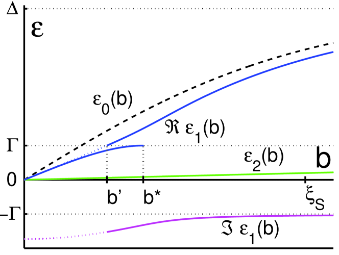
Figure 1: (Color online) Two-scale behavior of the spectrum, Eq. (9), for coherent tunneling. The spectrum has two localized branches, $\epsilon_{1}(b)$ and $\epsilon_{2}(b)$, for $\epsilon<\Gamma$. The branch $\epsilon_{2}(b)$ has a scale $\xi_{2D}$, it saturates at $\epsilon=\Gamma$ for $b\gg\xi_{2D}$. $\epsilon_{1}(b)$ has a scale $\xi_{S}$. For $\Re\epsilon>\Gamma$ it transforms into scattering resonances. $b^{*}$ is defined as $\epsilon_{1}(b^{*})=\Gamma-0$, while $b^{\prime}$ corresponds to $\Re\epsilon_{1}(b^{\prime})=\Gamma+0$.

Matching the 2D Green functions through the primary core region of rapidly changing self-energy potentials (see Appendix C) we find both the spectrum

$$q^{-1}[\epsilon-\epsilon_{2}(b)][\epsilon-\epsilon_{0}(b)]+\Gamma^{2}-\Gamma\sqrt{\Gamma^{2}-[\epsilon-\epsilon_{2}(b)]^{2}}=0$$ (9)

and the Green functions for trajectories with $b\ll\xi_{2D}$. Here $q=v_{\parallel}/V_{2D}$. For $b\lesssim\xi_{S}$, the cut-off parameter in Eq. (5) should be replaced with $\Lambda=\xi_{2D}/\xi_{S}$.

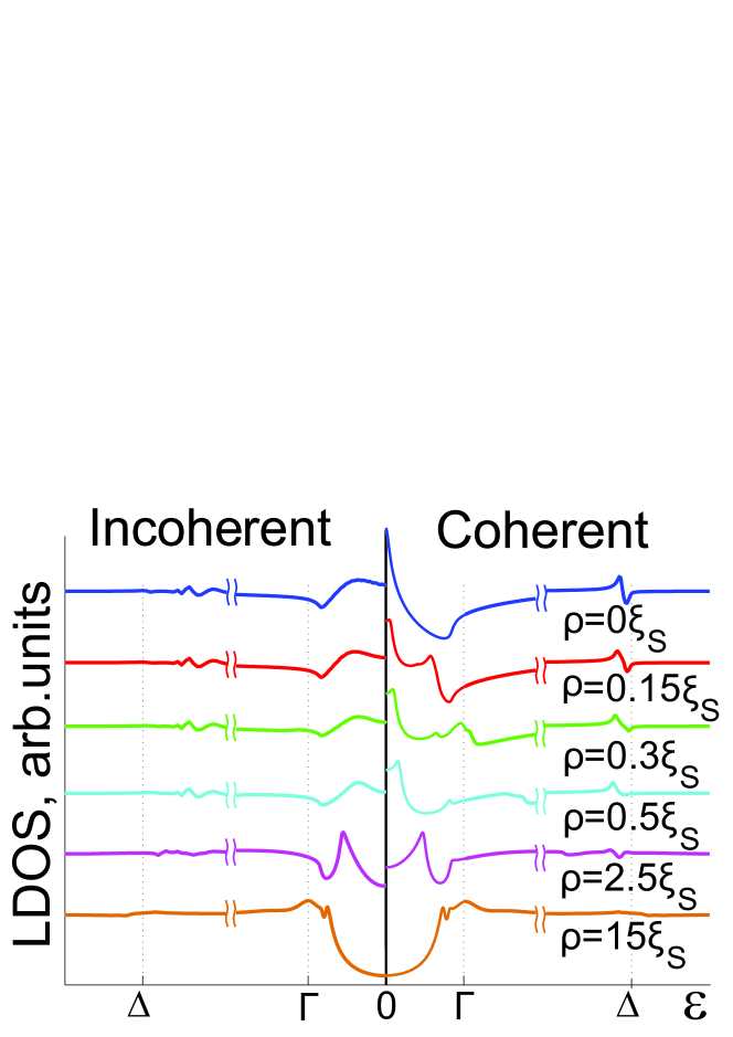
Figure 2: (Color online) The local DOS in logarithmic scale for coherent (right panel) and incoherent (left panel) tunneling in the clean limit for different distances $\rho$ from the vortex center. The peaks in LDOS exist up to distances $\sim\xi_{2D}$. Here $\Delta/\Gamma=5$, $q=1$.

The resulting two-scale behavior of the spectral branches is illustrated in Fig. 1. The complex-valued energy branches satisfy the symmetry condition: $\epsilon_{1,2}(-b)=-\epsilon^{*}_{1,2}(b)$. There are two real-valued energy branches in the range $|\epsilon|<\Gamma$ crossing zero of energy as functions of the impact parameter and one complex-valued branch in the range $\Gamma<|\epsilon|<\Delta_{\infty}$. The lowest-energy branch $\epsilon_{2}(b)$ as a function of the impact parameter has a characteristic scale $\xi_{2D}$: For $b\lesssim\xi_{2D}$ it is determined by Eq. (5) with the proper cut-off parameter $\Lambda$ as discussed above. On the other hand, it saturates at $\epsilon=\Gamma$ for $b>>\xi_{2D}$. The branch $\epsilon_{1}(b)$ has a scale $\xi_{S}$: At low energies it goes slightly below the CdGM spectrum $\epsilon_{0}(b)$ in the bulk SC, $\epsilon_{1}(b)=(1+q/2)^{-1}\epsilon_{0}(b)$. Above the induced gap $\Gamma$ the spectrum transforms into a scattering resonance due to the decay into the delocalized modes propagating in the 2D layer: $\epsilon_{1}(b)=\epsilon_{0}(b)-i\Gamma$ for $|\epsilon|\gg\Gamma$. Since Eq. (9) determines a pole of the retarded Green function in the lower half-plane of complex $\epsilon$, the square root in Eq. (9) should be analytically continued under the cut extending from $-\infty$ to $-\Gamma$ and from $\Gamma$ to $+\infty$. As a result, $\epsilon_{1}(b)$ has a discontinuity at $\epsilon_{1}=\Gamma$.

Two branches appear because the system under consideration consists of two sub-systems Shiozaki12 , the bulk SC and the 2D proximity layer, each with its own anomalous branch. The branch $\epsilon_{1}(b)$ is the proximity image of the bulk spectrum $\epsilon_{0}(b)$ with the spectral weight proportional to the tunneling probability $\Gamma$. The branch $\epsilon_{2}(b)$ belongs to the 2D layer itself. We note that the presence of two anomalous branches does not contradict to the index theorem Volovik . Indeed, its application requires that both zero of the quasiclassical Hamiltonian at the Fermi surface and its singularity at $\epsilon=\epsilon_{0}(b)$ are taken into account when calculating the topological invariant. As a result, the number of anomalous branches is increased up to 2 for a single-quantum vortex.

The multiple-branch spectrum results in multiple peaks in the LDOS energy dependence (right panel in Fig. 2). Here the local DOS is defined by the angle-resolved one (normalized by its normal state value) ${N_{\epsilon}(s,b)=[g^{R}(s,b)-g^{A}(s,b)]/2}$ averaged over the trajectory direction. The multiple peak structure appears to be most pronounced deeply inside the primary core region (at distances $\rho\lesssim\xi_{S}^{2}/\xi_{2D}$ when $\epsilon_{1}<\Gamma$) illustrating, thus, the two-scale structure of the vortex core.

The number of LDOS peaks at a certain distance $\rho$ from the vortex center is determined by the number of spectral branches at $b\sim\rho$. The spectrum discontinuity at the induced gap $\Gamma$ causes the appearance of three LDOS peaks in the range of distances, corresponding to $b^{\prime}<b<b^{*}$ (see the plot for $\rho=0.3\xi_{S}$ in Fig. 2). The numerical LDOS patterns have been obtained by the subsequent solving of two sets of Eilenberger equations in Riccati parametrization Schopohl : first, we calculated the Green functions for the bulk superconductor with the model order parameter profile $\Delta_{0}(\rho)=\Delta_{\infty}\rho/\sqrt{\rho^{2}+\xi_{S}^{2}}$ and, second, we have found the solution of Eq. (1) for a 2D layer with the induced potentials defined by the Eq. (2).

Multiple core. Clean limit with incoherent tunneling.

We proceed our study with the consideration of disorder effects and introduce first the momentum scattering during the tunneling process described within the incoherent tunneling model. Considering the tunneling as a perturbation one can assume a specular quasiparticle scattering at the interface and, thus, use the results of the previous section for the Green functions. The self-energy potentials in this case can be obtained by averaging of Eqs. (6-8) over the trajectory direction: $\check{\Sigma}_{T}=i\Gamma\left<\check{g}_{S}\right>$. This averaging does not affect, of course, the induced gap function (4) outside the primary vortex core and, thus, the spectrum $\epsilon_{2}$ survives the influence of the tunnel barrier disorder at least for $b>\xi_{S}$. On the contrary, the subgap branches localized within the primary vortex core region appear to be completely destroyed. Such dramatic consequence of the momentum scattering is caused by the averaging of electronic wave functions with different impact parameters and consequent loss of any information about the CdGM states of the primary vortex. A natural consequence of the momentum scattering is the appearance of a finite broadening of energy levels for trajectories with small impact parameters $b\lesssim\xi_{S}$.

Following again the matching procedure described above (see Appendix C) we find the angle-resolved DOS for $b\lesssim\xi_{S}$ and $|\epsilon|\ll\Gamma$,

$$N_{\epsilon}(s,b) = \frac{\Gamma\gamma(b)e^{-|s|/\xi_{2D}}}{[\epsilon-\epsilon_{2}(b)-\beta(b)]^{2}+\gamma^{2}(b)}\ ,$$ (10)

$$\beta(b) = \Gamma^{2}\left<\frac{\pi q}{Q\Omega}{\rm sign}(\epsilon+\Omega b)\right>_{z}\ ,$$ (11)

$$\gamma(b) = \Gamma^{2}\left<\frac{q}{Q\Omega}\ln\frac{\Delta_{\infty}}{|\Omega b+\epsilon|}\right>_{z}\ .$$ (12)

The angular brackets denote averaging over the momentum $p_{z}$ along the vortex axis in bulk SC, $\Omega=\partial\epsilon_{0}/\partial b$. The DOS has a peak of the height $\Gamma/\gamma$ at an energy ${\epsilon=\epsilon_{2}(b)+\beta(b)}$ shifted from a standard bound state level (see Appendix C.2 for details). This shift results in splitting of the zero-bias anomaly in LDOS, as is seen from our numerical analysis (see the left panel in Fig. 2). For LDOS calculations we use the numerical procedure similar to that used for the coherent limit above with the induced potentials averaged over the Fermi surface (assumed cylindrical) in the bulk.

Multiple core. Dirty superconductor with clean 2D layer.

Smearing of the energy dependence of the induced potentials caused by disorder becomes even stronger if the bulk SC has short mean free path: $\ell\ll\xi_{S}$. In dirty limit, the momentum averaged retarded (advanced) Green functions are parameterized as follows:

$$\check{g}_{S}^{R(A)}(\rho)=\check{\tau}_{3}\sin\Theta^{R(A)}+\check{\tau}_{2}\cos\Theta^{R(A)}e^{-i\check{\tau}_{3}\phi}\ .$$ (13)

We put $\Theta^{R(A)}=\pm\Theta_{1}+i\Theta_{2}$. The boundary conditions (4) require $\Theta_{1}\to\pi/2$, $\Theta_{2}\to 0$ for $\rho\to 0$. At large distances $\sin\Theta_{1}\to 0$, $\tanh\Theta_{2}\to-\epsilon/\Gamma$ for $\epsilon<\Delta_{\infty}$ while $\cos\Theta_{1}\to 0$, $\tanh\Theta_{2}\to-\Delta_{\infty}/\epsilon$ for $\epsilon>\Delta_{\infty}$. Therefore, $\Theta_{2}=0$ for $\epsilon\ll\Delta_{\infty}$, and the Usadel equation becomes GorkovKopnin

$$D_{S}\left[\nabla^{2}\Theta_{1}+\frac{\sin(2\Theta_{1})}{2\rho^{2}}\right]-2\Delta_{0}\sin\Theta_{1}=0$$ (14)

The solution of Eq. (14) has been found in Ref. GorkovKopnin : the function $\Theta_{1}(\rho)$ monotonously decays from $\pi/2$ at the origin down to the zero value at $\rho\gg\xi_{S}$. The Green functions (13) determine the induced vortex potentials $\check{\Sigma}_{T}=i\Gamma\check{g}_{S}$.

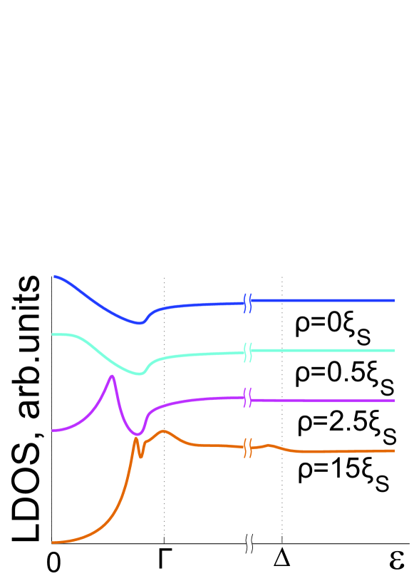
Figure 3: (Color online) The local DOS in logarithmic scale for the dirty limit with the parameters $\Delta/\Gamma=5$, $V_{2D}/V_{F}=1$ for different distances $\rho$ from the vortex center.

For $|\epsilon|\ll\Gamma$ and $b\lesssim\xi_{S}$ the peak in the energy dependence of the angle-resolved DOS is described by the Eq.(10) with $\beta=0$ and

$$\gamma=\frac{2\Gamma^{2}}{\hbar V_{2D}}\int_{0}^{\infty}\sin\Theta_{1}\,ds$$ (15)

(see Appendix C.3 for details). The numerical results clearly confirm the existence of one broadened peak in the LDOS dependence vs energy: this peak shifts with the increasing distance from the vortex center and becomes sharper (see Fig. 3). Our numerical procedure of the LDOS calculation in this limit is based on the using of a standard relaxation method RelaxMethod for solving the Usadel equation Golubov in the bulk SC and Riccati parametrization for Eilenberger equations in the 2D layer.

Vortex core expansion. Dirty superconductor and 2D layer.

To complete our analysis we discuss the case of strong disorder both in the bulk superconductor and in the 2D layer. This limit has been previously studied in Ref. Golubov-vortex . As before, one can parameterize the Green functions averaged over the 2D momentum directions in the form of Eq. (13), where we use $\Psi$ for the 2D-layer functions instead of $\Theta$. The boundary conditions coincide with those for Eq. (13) where $\Delta_{\infty}$ is replaced with $\Gamma$. With the self energies from the previous subsection, the Usadel equation for the retarded function for $\epsilon\ll\Delta_{\infty}$ is

$$D_{2D}\left[\nabla^{2}\Psi+\frac{\sin(2\Psi)}{2\rho^{2}}\right]-2\Gamma\sin(\Psi-\Theta)-2i\epsilon\cos\Psi=0.$$ (16)

$\Theta$ is essentially nonzero only inside the primary core region $\rho<\xi_{S}$. The condition $\xi_{S}\ll\xi_{2D}=\sqrt{\hbar D_{2D}/\Gamma}$ ensures that such short-distance inhomogeneity in the induced vortex potentials does not disturb the adiabatic solution based on Eq. (4) (see Appendix C.4). Thus, putting $\Theta=0$ in Eq. (16) we reduce our problem to that describing a standard vortex in a dirty superconductor with the gap value $\Gamma$. Thus, the full disordered system should reveal the same LDOS patterns as in the bulk case, though scaled with the much larger coherence length $\xi_{2D}$ instead of $\xi_{S}$. This conclusion is, of course, in agreement with numerical calculations in the Ref. Golubov-vortex .

Conclusion

To summarize, we calculate the electronic structure of a proximity induced vortex core in a 2D metallic layer covering a superconducting half-space. We predict formation of a multiple vortex core resulting in a two-scale behavior of the LDOS. For coherent tunneling between the 2D layer and the bulk superconductor, the spectrum has two subgap branches while for incoherent tunneling only one of them remains. The splitting of the zero-bias anomaly and the multiple peak structure in the LDOS should be visible in the tunneling spectroscopy experiments. Disorder further smears the multiple peak structure inside the double-scale vortex core. When both the bulk SC and the 2D layer are in dirty limits, the 2D LDOS qualitatively repeats that in the bulk SC scaled with the larger coherence length $\xi_{2D}$. Such expansion of the vortex core probably relates to the anomalously large vortex images observed in $MgB_{2}$ eskildsen and high– $T_{c}$ cuprates yeh .

We thank A. Buzdin and G. Volovik for stimulating discussions. This work was supported in part by the Academy of Finland, Centers of excellence program 2012–2017, by the Russian Foundation for Basic Research, by the Program “Quantum Physics of Condensed Matter” of the Russian Academy of Sciences, and by FTP “Scientific and educational personnel of innovative Russia in 2009-2013”.

Appendix A Eilenberger equations for coherent and incoherent models

We start with the equation for the retarded (advanced) Green functions derived in Ref. KopninMelnikov11

$$\check{G}^{-1}({\bf r}_{1})\check{G}_{2D}({\bf r}_{1},{\bf r}_{2},\epsilon)-\!\!\int\check{\Sigma}_{T}({\bf r}_{1},{\bf r}^{\prime})\check{G}_{2D}({\bf r}^{\prime},{\bf r}_{2},\epsilon)\,d^{2}r^{\prime}\\ =\check{1}d^{-1}\delta({\bf r}_{1}-{\bf r}_{2})\ .\;$$ (17)

Here $d$ is the layer thickness, $\check{\tau}_{1}$, $\check{\tau}_{2}$, and $\check{\tau}_{3}$ as well as

$$\check{G}_{2D}=\left(\begin{array}[]{cc}G&F\\ -F^{\dagger}&\widetilde{G}\end{array}\right)\ ,\;\check{G}^{-1}({\bf r}_{1})=\epsilon_{2D}(\hat{\bf p})-\mu-\epsilon\check{\tau}_{3}\ ,$$

are matrices in the Nambu space, $\epsilon_{2D}(\hat{\bf p})$ is the spectrum of the 2D electron system, $\hat{\bf p}=-i\hbar{\bm{\nabla}}$ and ${\bf r}$ are the 2D momentum and coordinate, correspondingly. The self-energy takes the form,

$$\check{\Sigma}_{T}({\bf r}_{1},{\bf r}_{2})=d\,t({\bf r}_{1})\check{G}_{S}({\bf r}_{1},z_{1}=0;{\bf r}_{2},z_{2}=0)t({\bf r}_{2})$$ (18)

where $t({\bf r})$ is the tunneling amplitude which is assumed real and the Green function $G_{S}$ of the bulk SC is taken at the SC/2D interface $z=0$. The above equations can be strongly simplified using a standard quasiclassical procedure which allows us to derive the Eilenberger equations for quasiclassical Green function

$$\check{g}({\bf p}_{2D},{\bf r})=({\pi i})^{-1}\int{d\xi_{2}}\check{G}_{2D}({\bf p},{\bf r})$$

Here we derive expressions for the self energies (2, 3) and the Eilenberger equations (1) for different tunneling models.

A.1 Coherent tunneling

Let us assume that the in-plane momentum projection is conserved during the tunneling process. This amounts for a tunneling amplitude $t({\bf r})$ independent of the coordinate along the SC/2D interface. In 2D momentum representation the self energy in Eq. (17) becomes

$$\check{\Sigma}_{T}({\bf p}_{1},{\bf p}^{\prime})=dt^{2}\int\check{G}_{S}({\bf p}_{1},p_{z};{\bf p}^{\prime},p_{z}^{\prime})\frac{dp_{z}\,dp_{z}^{\prime}}{(2\pi)^{2}}\ .$$

We now apply the operators to the Green function from the right and subtract this equation from Eq. (17). Integrating the result over the energy variable near the Fermi surface $\xi_{2}=\epsilon_{2D}({\bf p})-\mu$ and using

$$\int\frac{d\xi_{2}}{\pi i}\int\check{\Sigma}_{T}({\bf p}_{1},{\bf p}^{\prime})\check{G}_{2D}({\bf p}^{\prime},{\bf p}_{2})\frac{d^{2}p^{\prime}}{(2\pi)^{2}}=dt^{2}g({\bf p}_{2D},{\bf r})\\ \times\int\frac{dp_{z}}{2\pi}\check{g}_{S}({\bf p}_{2D},p_{z};{\bf r},0)\,\pi i\delta_{\Delta}\left[\epsilon_{S}({\bf p}_{2D},p_{z})-\mu\right]$$

we obtain the quasiclassical Eilenberger equation (1). The quasiclassical Green function $\check{g}_{S}({\bf p};{\bf r},0)$ of the bulk SC is taken at the SC/2D interface ${z=0}$. We use the mixed momentum ${\bf p}$-coordinate ${\bf r}$ representation describing the relative and center-of-mass motion of electrons in the Cooper pair and put

$$\check{\mathcal{G}}_{S}({\bf p},p_{z};{\bf r},z) = \check{g}_{S}({\bf p},p_{z};{\bf r},z)\pi i\delta_{\Delta}(\xi_{3})\ ,$$

$$\check{\mathcal{G}}_{2D}({\bf p},{\bf r}) = \check{g}({\bf p},{\bf r})\pi i\delta_{\Delta}(\xi_{2})\ .$$

Here $\xi_{3}=\epsilon_{S}({\bf p},p_{z})-\mu$ is the normal quasiparticle spectrum in the 3D half-space, $\check{g}_{S}$ and $\check{g}$ are standard quasiclassical Green functions, and $\delta_{\Delta}(\xi_{2,3})$ is a delta function broadened at the gap energy scale $\Delta$.

Assuming isotropic Fermi surfaces in both the superconductor and the 2D layer we get the self energy in the form of Eq. (2) with the tunneling rate

$$\Gamma=dt^{2}\int\limits_{0}^{\infty}\delta_{\Delta}\left[\epsilon_{S}({\bf p}_{2D},p_{z})-\mu\right]dp_{z}\ .$$

Provided the 2D Fermi surface is smaller than the extremal cross section of the 3D Fermi surface, i.e., $p_{2D}<p_{F}$ the expression for the tunneling rate reads: ${\Gamma=dmt^{2}/p_{3z}}$. For large 2D Fermi surfaces $p_{2D}>p_{F}$ the self energy term vanishes, and the coherent tunneling is impossible. The case of close momenta $p_{2D}\simeq p_{F}$ deserves special consideration which should take account of a finite delta function width: $\Gamma\sim dt^{2}(m/\Delta)^{1/2}$.

A.2 Incoherent tunneling

We now assume that the tunneling occurs through random centers such that the ensemble average of amplitudes in Eq. (18) is

$$\left<t({\bf r}_{1})t({\bf r}_{2})\right>=t^{2}s_{a}\delta({\bf r}_{1}-{\bf r}_{2})\ ,$$ (19)

where $s_{a}$ is the correlated area of the order of atomic scale. After averaging the self energy becomes:

$$\check{\Sigma}_{T}({\bf r}_{1},{\bf r}_{2})=t^{2}ds_{a}\check{G}_{S}({\bf r}_{1},{\bf r}_{1};0)\delta({\bf r}_{1}-{\bf r}_{2})$$

$$=t^{2}ds_{a}i\pi\nu_{3}(0)\left<\check{g}_{S}({\bf p};{\bf r},0)\right>\delta({\bf r}_{1}-{\bf r}_{2})\ .$$

Here $\nu_{3}(0)$ is the normal density of states in the bulk material. Angular brackets denote averaging over three-dimensional momentum directions. Within the quasiclassical approach the resulting self energy is given by Eq. (3) with the tunneling rate $\Gamma=\pi\nu_{3}(0)ds_{a}t^{2}$. This approximation coincides with that used in Ref. KopninMelnikov11 .

Appendix B Induced vortex potentials

In both tunneling models the Green functions of the 2D layer satisfy the Eilenberger equations (1):

$$-i\hbar{\bf v}_{2D}{\bm{\nabla}}f-2\left[\epsilon+\Sigma_{1}\right]\!f+2\Sigma_{2}g=0,\;$$ (20)

$$i\hbar{\bf v}_{2D}{\bm{\nabla}}f^{\dagger}-2\left[\epsilon+\Sigma_{1}\right]\!f^{\dagger}+2\Sigma_{2}^{\dagger}g=0,\;$$ (21)

$$-i\hbar{\bf v}_{2D}{\bm{\nabla}}g+\Sigma_{2}f^{\dagger}-\Sigma^{\dagger}_{2}f=0.\;$$ (22)

and the normalization condition $g^{2}-ff^{\dagger}=1$ with the self energy (2, 3) as effective potentials

$$\check{\Sigma}_{T}=\begin{pmatrix}\Sigma_{1}&\Sigma_{2}\\ -\Sigma^{\dagger}_{2}&-\Sigma_{1}\end{pmatrix}\ .$$

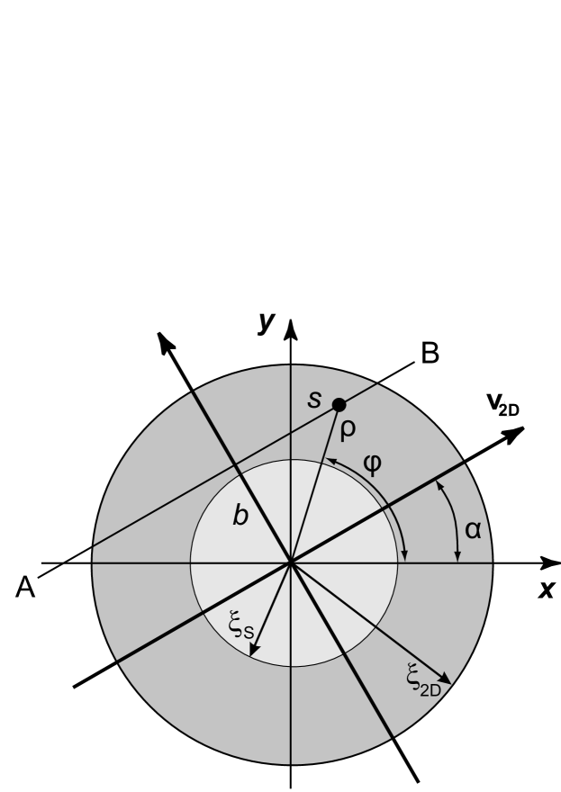
Figure 4: (Color online) The coordinate frame near the multiple vortex core. Primary (induced) core is shown by the white (gray) circle. The quasiparticle trajectory with an impact parameter $b$ (line AB) passes through the point $(\rho,\phi)$ shown by the black dot.

Quasiparticles are conveniently described by the coordinates along their trajectories (see Fig. 4). A quasiclassical trajectory is parameterized by its angle $\alpha$ with the $x$ axis, the impact parameter $b=\rho\sin(\phi-\alpha)$ and the coordinate $s=\rho\cos(\phi-\alpha)$ along the trajectory. We introduce the symmetric and antisymmetric parts of the Green functions KramerPesch ; Kopnin-book :

$$f=-\left[\zeta(s)+i\theta(s)\right]\exp(i\alpha)$$ (23a)

$$f^{\dagger}=\left[\zeta(s)-i\theta(s)\right]\exp(-i\alpha),$$ (23b)

where $\zeta(s)=\zeta(-s)$, and $\theta(s)=-\theta(-s)$. The normalization condition requires $g^{2}+\theta^{2}+\zeta^{2}=1$. Eilenberger equations (20-22) can be rewritten as follows:

$$\hbar V_{2D}\frac{d\zeta}{ds}+2\left(\epsilon+\Sigma_{1}\right)\theta-2ig\Sigma_{R} =0,\quad$$ (24)

$$\hbar V_{2D}\frac{d\theta}{ds}-2\left(\epsilon+\Sigma_{1}\right)\zeta-2ig\Sigma_{I} =0,\quad$$ (25)

$$\hbar V_{2D}\frac{dg}{ds}+2i\zeta\Sigma_{R}+2i\theta\Sigma_{I} =0,\quad$$ (26)

where

$$2\Sigma_{R}=\left(\Sigma_{2}e^{-i\alpha}+\Sigma_{2}^{\dagger}e^{i\alpha}\right),\quad$$ (27a)

$$2i\Sigma_{I}=\left(\Sigma_{2}e^{-i\alpha}-\Sigma_{2}^{\dagger}e^{i\alpha}\right).\quad$$ (27b)

In order to evaluate the induced vortex potentials $\Sigma_{1}$, $\Sigma_{2}$ and $\Sigma_{2}^{\dagger}$ we start from two important assumptions: (i) low interface barrier transparency and (ii) negligible effect of the diffusive interface reflection. These assumptions allow us to neglect the effect of tunneling on the bulk superconductor characteristics and use the bulk values of the quasiclassical Green functions. Restricting our consideration to the small energy values $\epsilon\ll\Delta_{\infty}$ we find the large-scale ($\rho\gg\xi_{S}$) self energy (4) to be independent of the particular tunneling model and disorder rate in the bulk SC: $\Sigma_{1}=i\Gamma g_{S}\approx 0$, $\Sigma_{2}=i\Gamma f_{S}\approx\Gamma e^{i\phi}$, i.e. $\Sigma_{R}\approx\Gamma s/\rho$, $\Sigma_{I}\approx\Gamma b/\rho$.

Contrary to the large distance limit the induced vortex potentials close to the primary vortex core reveal a very peculiar behavior depending on impurity concentration and momentum conservation during the tunneling process. In a clean limit of the bulk SC we use the Green function parametrization similar to (23) and rewrite the Eilenberger equations in the following form:

$$\hbar v_{\parallel}{\frac{{\partial\zeta_{S}}}{{\partial s}}}+2\epsilon\theta_{S}-2i\Delta_{0}g_{S}s/\rho = 0,$$ (28)

$$\hbar v_{\parallel}{\frac{{\partial\theta_{S}}}{{\partial s}}}-2\epsilon\zeta_{S}-2i\Delta_{0}g_{S}b/\rho = 0.$$ (29)

For energies $\epsilon\ll\Delta_{\infty}$, the functions $g_{S}$ and $f_{S}$, $f^{\dagger}_{S}$ are large near the vortex. Assuming that $\zeta_{S}^{2}\gg\theta_{S}^{2}-1$, we have $g_{S}^{R(A)}=i\zeta_{S}^{R(A)}$. The plus sign here is chosen to satisfy the condition of vanishing $g_{S}$ at large distances according to Eq. (4). The solution of Eqs. (28, 29) for retarded and advanced Green functions KramerPesch ; Kopnin-book

$$\zeta_{S}^{R(A)} = \frac{\hbar v_{\parallel}e^{-K}}{2Q\left[\epsilon\pm i\delta-\epsilon_{0}\right]}\ ,\;$$ (30)

$$\theta_{S}^{R(A)} = \frac{2}{\hbar v_{\parallel}}\int_{0}^{s}(\epsilon-\Delta_{0}b/\rho)\zeta_{S}^{R(A)}ds^{\prime}\ ,\;$$ (31)

coincides with (6-8). These expressions hold as long as $|\zeta_{S}|$ exceeds $|b|/\rho$. For $s\gg\xi_{S}$ the function $\zeta_{S}$ assumes its asymptotic expression $\zeta^{R(A)}_{S}=-b/\rho$ corresponding to the boundary conditions (4).

In the clean limit the vortex potentials induced in the 2D layer are crucially dependent on tunneling model. Assuming specular quasiparticle reflection at the superconductor surface we put $\check{g}_{S}(+p_{z})=\check{g}_{S}(-p_{z})$ in Eq. (2) so that the self energy coincides with the Green function in the bulk for coherent tunneling $\Sigma_{1}=i\Gamma g_{S}$, $\Sigma_{2}=i\Gamma f_{S}$ and with its values averaged over the ensemble for the incoherent one: $\Sigma_{1}=i\Gamma\left<g_{S}\right>$, $\Sigma_{2}=i\Gamma\left<f_{S}\right>$. The ensemble averaging in terms of quasiclassical Green functions is equivalent to the averaging over the 3D momentum direction. One can separate two terms in the Green function expressions:

$$g^{R(A)}=i\zeta^{R(A)}=\wp\frac{i\hbar v_{\parallel}e^{-K}}{2Q\left[\epsilon-\epsilon_{0}\right]}\pm\frac{\pi\hbar v_{\parallel}e^{-K}}{2Q}\delta(\epsilon-\epsilon_{0})\ .$$ (32)

The first term has to be taken as a principal value integral when calculating the angular averages. The second term is proportional to the delta function of energy and determines the density of states (DOS) of the vortex core states in the bulk SC. Similarly, the anomalous functions

$$f^{R(A)}=e^{i\phi}(i\zeta^{R(A)}-\theta^{R(A)})[b+is]/\rho\ ,$$ (33)

$$f^{\dagger R(A)}=e^{-i\phi}(i\zeta^{R(A)}+\theta^{R(A)})[b-is]/\rho\ .$$ (34)

can be separated into the principal value part and the delta-functional contribution.

Performing averaging over the polar $\theta_{p}$ and azimuthal $\alpha$ angles we take into account the symmetry of the functions under the $s$-inversion transformation. Thus, we find the following expressions for the self energy terms:

$$\Sigma_{1} = -\Gamma\left<\zeta_{S}(s)\right>$$ (35)

$$\Sigma_{2}e^{-i\phi}=\Sigma_{2}^{\dagger}e^{i\phi} = \Gamma\left<\theta_{S}(s)s-\zeta_{S}(s)b\right>/{\rho}\ .$$ (36)

It is convenient to split the off-diagonal induced potential into the localized ($\Sigma_{2}^{loc}$) and the long-range parts:

$$\Sigma_{2}e^{-i\phi} = \Gamma\Phi+\Sigma_{2}^{loc}\ ,$$ (37)

$$\Phi(\rho) = \wp\left<\,{I(s){\rm sign}(s)}/{2Q\left[\epsilon-\epsilon_{0}\right]}\right>\ .$$ (38)

Here we put $I(s)=2\int_{0}^{s}(\epsilon-\Delta_{0}b/\rho)e^{-K(s^{\prime})}\,ds^{\prime}$. The long-range function $\Phi$ can be regarded as an adiabatic induced superconducting gap. Hereafter we focus on the evaluation of the localized part which is most important in the primary core region. Averaging over the azimuthal trajectory angle $\alpha$ we find:

$$\Re\Sigma_{2}^{loc} = \Gamma\left<\frac{\hbar v_{\parallel}e^{-K}}{2Q\Omega\rho}\left[1-\frac{|\epsilon|}{\sqrt{\epsilon^{2}-\Omega^{2}\rho^{2}}}\chi(\epsilon^{2}-\Omega^{2}\rho^{2})\right]\right>_{z}\ ,$$

$$\Im\Sigma_{2}^{loc} = \pm\Gamma\left<\frac{\epsilon\hbar v_{\parallel}e^{-K}}{2Q\rho\Omega\sqrt{\Omega^{2}\rho^{2}-\epsilon^{2}}}\chi(\Omega^{2}\rho^{2}-\epsilon^{2})\right>_{z}\ ,$$

$$\Re\Sigma_{1} = -{\rm sign}(\epsilon)\Gamma\left<\frac{\hbar v_{\parallel}e^{-K}}{2Q\sqrt{\epsilon^{2}-\Omega^{2}\rho^{2}}}\chi(\epsilon^{2}-\Omega^{2}\rho^{2})\right>_{z}\ ,$$

$$\Im\Sigma_{1} = \pm\Gamma\left<\frac{\hbar v_{\parallel}e^{-K}}{2Q\sqrt{\Omega^{2}\rho^{2}-\epsilon^{2}}}\chi(\Omega^{2}\rho^{2}-\epsilon^{2})\right>_{z}\ .$$

Here the upper (lower) sign corresponds to a retarded (advanced) self energy term, $\Omega=d\epsilon_{0}/db$,

$$\chi(x)=\left\{1,\quad x>1\atop 0,\quad x<1\right.$$

is the Heaviside theta-function, and we use the notation

$$\left<\ldots\right>_{z}=\frac{1}{2}\int_{0}^{\pi}\sin\theta_{p}d\theta_{p}\left(\ldots\right)$$

for the average over the polar angle $\theta_{p}$ of the 3D Fermi momentum. Note that our calculations are essentially based on the first-order approximation in the small parameter $b/\rho$. According to Eq. (27) the symmetrical $\Sigma_{I}(-s)=\Sigma_{I}(s)$ and antisymmetrical $\Sigma_{R}(-s)=-\Sigma_{R}(s)$ parts of the off-diagonal self energy term $\Sigma_{2}e^{-i\phi}$ can be rewritten as follows: $\Sigma_{R}=\Sigma_{2}e^{-i\phi}s/\rho$ and $\Sigma_{I}=\Sigma_{2}e^{-i\phi}b/\rho$.

Appendix C Scale separation inside the multiple vortex core.

In this Appendix we present the details of the analytical procedure used to match the solutions of quasiclassical equations through the primary core region. In a clean 2D layer we start our consideration of the induced vortex states from the Eilenberger equations (24-26) for retarded and advanced Green functions. In the low energy limit $\epsilon\ll\Delta_{\infty}$ appropriate boundary conditions far from the induced vortex core ($\rho\gg\xi_{2D}$) take the form:

$$\theta = \frac{\Gamma s/\rho}{\sqrt{\Gamma^{2}-\epsilon^{2}}}\ ,\;\zeta=\frac{-\Gamma b/\rho}{\sqrt{\Gamma^{2}-\epsilon^{2}}}\ ,g=\frac{-i\epsilon}{\sqrt{\Gamma^{2}-\epsilon^{2}}}\ .$$ (39)

The self energy terms reveal a quite different behavior in the small ($\rho\lesssim\xi_{S}$) and large ($\rho\gg\xi_{S}$) distance regions. To match the solutions in these domains we introduce a certain distance $\rho_{0}$ such that $\xi_{S}\ll\rho_{0}\ll\xi_{2D}$ and consider the Green functions in two overlapping spatial intervals: (i) $\rho<\rho_{0}\ll\xi_{2D}$ and (ii) $\rho\gg\xi_{S}$.

Outside the primary core region $\rho\gg\xi_{S}$ Eqs. (24-26) for both tunneling models and arbitrary disorder rate inside the superconductor take the form:

$$\hbar V_{2D}\frac{d\zeta}{ds}+2\epsilon\theta-2ig\Gamma s/\rho=0,$$ (40)

$$\hbar V_{2D}\frac{d\theta}{ds}-2\epsilon\zeta-2ig\Gamma b/\rho=0,$$ (41)

$$\hbar V_{2D}\frac{dg}{ds}+2i\theta\Gamma b/\rho+2i\zeta\Gamma s/\rho=0\ .$$ (42)

The functions $g$ and $\zeta$ are even in $s$ while $\theta$ is odd, so we can consider only positive $s$ values. We obtain the solution of the above equations using the first order perturbation theory in the impact parameter $b$: $\check{w}(s)=\check{w}_{0}(s)+\check{w}_{1}(s)$, where $\check{w}(s)=\left(\zeta,\theta,g\right)^{T}$. This approximation holds for $|b|\ll\xi_{2D}$. The zero order in $b$ solution reads

$$\check{w}_{0}(s)=\frac{1}{\sqrt{\Gamma^{2}-\epsilon^{2}}}\check{u}_{0}(s)+\frac{C}{\sqrt{\Gamma^{2}-\epsilon^{2}}}\check{u}_{-}(s)\ ,$$ (43)

where

$$\check{u}_{\pm}(s)=\left(\begin{array}[]{c}\sqrt{\Gamma^{2}-\epsilon^{2}}\\ \pm\epsilon\\ \mp i\Gamma\end{array}\right)e^{\pm\lambda s}\ ,$$

$$\check{u}_{0}(s)=\left(\begin{array}[]{c}0\\ \Gamma\\ -i\epsilon\end{array}\right)\ ,\,\lambda=\frac{2\sqrt{\Gamma^{2}-\epsilon^{2}}}{\hbar V_{2D}}$$

This solution satisfies the boundary conditions $g=-i\epsilon/\sqrt{\Gamma^{2}-\epsilon^{2}}$, $\zeta=0$ and $\theta=\Gamma/\sqrt{\Gamma^{2}-\epsilon^{2}}$ for $s\to\infty$ and $\epsilon^{2}<\Gamma^{2}$. The first order correction $\check{w}_{1}$ can be written as

$$\check{w}_{1}(s)=\frac{C_{0}(s)}{\sqrt{\Gamma^{2}-\epsilon^{2}}}\check{u}_{0}+\frac{C_{+}(s)}{\sqrt{\Gamma^{2}-\epsilon^{2}}}\check{u}_{+}+\frac{C_{-}(s)}{\sqrt{\Gamma^{2}-\epsilon^{2}}}\check{u}_{-}\ ,$$ (46)

where

$$\xi_{2D}C_{0}(s)=2Cb\int_{s}^{\infty}e^{-\lambda s}\frac{ds}{\rho}\ ,$$ (47)

$$\xi_{2D}C_{+}(s)=-b\int_{s}^{\infty}e^{-\lambda s}\frac{ds}{\rho}\ ,$$ (48)

$$\xi_{2D}C_{-}(s)=-b\int_{s_{c}}^{s}e^{\lambda s}\frac{ds}{\rho}\ .$$ (49)

The lower limit of integration $s_{c}$ in $C_{-}$ has to be taken $s_{c}\sim\xi_{S}$ for trajectories that go through the primary vortex core, $b\lesssim\xi_{S}$, so that the logarithmic divergence is cut off at the distances $\sim\xi_{S}$ where the long-range vortex potential $\Phi$ (38) vanishes. For $b\gg\xi_{S}$ we have $s_{c}=0$. The perturbation approach holds as long as $C_{0}\ll C$ and $C_{+}\ll 1$, i.e., as long as $|b|\ll\xi_{2D}$. For $s\gg\xi_{2D}$ the coefficient $C_{0}$ decays faster than exponentially, while

$$C_{+}(s)e^{\lambda s}\to C_{-}(s)e^{-\lambda s}\to-\frac{\Gamma}{2\sqrt{\Gamma^{2}-\epsilon^{2}}}\frac{b}{\rho}$$

such that $\zeta$ is $-(b/\rho)\Gamma/\sqrt{\Gamma^{2}-\epsilon^{2}}$ and the corrections to $\theta$ and $g$ vanish as it should be according to (39). For a small distance $s=s_{0}$ ($\rho_{0}^{2}=s_{0}^{2}+b^{2}$) we have

$$\zeta(s_{0}) = C+C_{+}(s_{0})+C_{-}(s_{0}),$$ (50)

$$\theta(s_{0}) = \frac{1}{\sqrt{\Gamma^{2}-\epsilon^{2}}}\left[\Gamma-\epsilon C+\Gamma C_{0}(s_{0})\right.$$ (51)

$$+\left.\epsilon[C_{+}(s_{0})-C_{-}(s_{0})]\right],\quad$$

$$g(s_{0}) = \frac{i}{\sqrt{\Gamma^{2}-\epsilon^{2}}}\left[-\epsilon+\Gamma C-\epsilon C_{0}(s_{0})\right.$$ (52)

$$-\left.\Gamma[C_{+}(s_{0})-C_{-}(s_{0})]\right].\quad$$

Consider first trajectories that miss the primary vortex core, i.e., they go at impact parameters $\xi_{S}\ll b\ll\xi_{2D}$. In this case, the perturbation result Eqs. (40-42) can be applied along the entire trajectory such that one can put $s_{0}=s_{c}=0$. The boundary condition for an odd function requires $\theta(0)=0$. Since in this case $C_{-}(0)=0$, we find from Eq. (51)

$$\Gamma+\epsilon C_{+}(0)=\epsilon C-\Gamma C_{0}(0)\ .$$

Expressing the coefficients $C_{0}$ and $C_{+}$ in terms of the energy $\epsilon_{2}(b)$ of bound states in the induced vortex core, $C_{0}=-2CC_{+}=C\epsilon_{2}(b)/\Gamma$, we find

$$C[\epsilon-\epsilon_{2}(b)]=\Gamma-\epsilon\epsilon_{2}(b)/2\Gamma\ ,$$ (53)

where the energy spectrum $\epsilon_{2}(b)$ of localized excitations is given by the Eq. (5). According to Eq. (53) $\epsilon_{2}(b)$ is the only spectrum branch in the energy interval $|\epsilon|\ll\Delta_{\infty}$. The Green function is

$$g(s)=\frac{-i\epsilon}{\sqrt{\Gamma^{2}-\epsilon^{2}}}+\frac{i\Gamma C}{\sqrt{\Gamma^{2}-\epsilon^{2}}}e^{-\lambda s}-\frac{i\epsilon C_{0}(s)}{\sqrt{\Gamma^{2}-\epsilon^{2}}}\\ -\frac{i\Gamma}{\sqrt{\Gamma^{2}-\epsilon^{2}}}\left[C_{+}(s)e^{\lambda s}-C_{-}(s)e^{-\lambda s}\right]\ .$$ (54)

For $s\gg\xi_{2D}$ we have $C_{0}\to 0$, $C_{+}e^{\lambda s}-C_{-}e^{-\lambda s}\to 0$, so that the first term is the homogeneous background while the rest terms describe the vortex contribution. To obtain the retarded function for $\epsilon^{2}>\Gamma^{2}$ one has to continue $\sqrt{\Gamma^{2}-\epsilon^{2}}$ analytically throughout the upper half-plane of complex $\epsilon$ keeping $\Re\sqrt{\Gamma^{2}-\epsilon^{2}}>0$.

The normalized LDOS can be found as a sum over different trajectories:

$$N({\bf r},\epsilon)=\frac{1}{2\pi}\int\limits_{0}^{2\pi}N_{\epsilon}(s,b)d\alpha^{\prime}\ ,$$

where $s=\rho\cos\alpha^{\prime}$, $b=-\rho\sin\alpha^{\prime}$, and

$$N_{\epsilon}(s,b)=\frac{1}{2}\left(g^{R}(s,b)-g^{A}(s,b)\right)\ .$$

For $|\epsilon|<\Gamma$, a nonzero LDOS comes only from the vortex contribution of the second and third terms in (54) due to the presence of a pole in the coefficient $C$ according to Eq. (53). The Green functions and LDOS reach their long-distance values $g=-i\epsilon/\sqrt{\Gamma^{2}-\epsilon^{2}}$ and $N=|\epsilon|/\sqrt{\epsilon^{2}-\Gamma^{2}}\chi(\epsilon^{2}-\Gamma^{2})$ as $\rho\to\infty$. For $\rho\gg\xi_{S}$ the trajectories with large impact parameters $b\gtrsim\xi_{S}$ give the main contribution to the LDOS. In the region ${\xi_{S}\ll\rho\ll\xi_{2D}}$ we get the angle–resolved density of states in the form:

$$N_{\epsilon}(s,b) = \frac{\sqrt{\Gamma^{2}-\epsilon^{2}}(\Gamma^{2}-\epsilon^{2}/2)}{\Gamma^{2}}$$ (55)

$$\times\pi\delta[\epsilon-\epsilon_{2}(b)]\ ,\phantom{223ispace}|\epsilon|<\Gamma$$

$$N_{\epsilon}(s,b) = \frac{\sqrt{\epsilon^{2}-\Gamma^{2}}[\Gamma^{2}-\epsilon_{2}^{2}(b)/2]}{{\rm sign}(\epsilon)\Gamma^{2}[\epsilon-\epsilon_{2}(b)]}\ ,\;|\epsilon|>\Gamma\ .$$ (56)

Thus, the corresponding LDOS in the energy interval $|\epsilon|<\Gamma$ has the only peaks at $\epsilon=\epsilon_{2}(\pm\rho)$:

$$N(\rho,\epsilon)=\frac{1}{\pi}\int\limits_{-\rho}^{\rho}N_{\epsilon}(\sqrt{\rho^{2}-b^{2}},b)\frac{db}{\sqrt{\rho^{2}-b^{2}}}=\\ =\frac{\sqrt{\Gamma^{2}-\epsilon^{2}}(1-\epsilon^{2}/2\Gamma^{2})}{\sqrt{\epsilon_{2}^{2}(\rho)-\epsilon^{2}}}\chi\left[\epsilon_{2}^{2}(\rho)-\epsilon^{2}\right]\ .$$ (57)

For energies above the induced gap, $|\epsilon|>\Gamma$, for the same distances the LDOS is monotonically increasing with $|\epsilon|$ to its normal state value:

$$N(\rho,\epsilon)=\sqrt{\epsilon^{2}-\Gamma^{2}}\left[\frac{|\epsilon|}{2\Gamma^{2}}+\frac{(1-\epsilon^{2}/2\Gamma^{2})}{\sqrt{\epsilon^{2}-\epsilon_{2}^{2}(\rho)}}\right]\ .$$ (58)

The LDOS behavior for small distances $\rho\lesssim\xi_{S}$ depends crucially on trajectories with small impact parameters $b$. In this case one has to match Eqs. (50)-(52) with the solution obtained in the vortex core region. For small $s<s_{0}$ we assume the even parts of the Green function $g$ and $\zeta$ to be nearly constant, therefore integrating Eq. (25) along the trajectory over $s$ from $0$ to $s_{0}$ we find the matching condition for the Green functions:

$$\frac{\hbar V_{2D}}{2}\theta(s_{0})=\zeta(s_{0})\int_{0}^{s_{0}}\Sigma_{1}\,ds+ig(s_{0})\int_{0}^{s_{0}}\Sigma_{I}\,ds\ .$$ (59)

This matching condition determines the constant $C$. Its poles as a function of energy and the impact parameter define the eigenstates of excitations.

While deriving the effective boundary condition (59) for $b\lesssim\xi_{S}$, one needs to separate the exponentially converging parts $\Sigma_{1,I}^{loc}$ at $s\sim\xi_{S}$ from the long-distance, $s\gg\xi_{S}$, asymptotics of $\Sigma_{1,I}$. For $\epsilon\ll\Delta_{\infty}$ the long-distance expressions, Eq. (4) yield $\Sigma_{1}=0$, $\Sigma_{R}=\Gamma s/\rho$, $\Sigma_{I}=\Gamma b/\rho$. Therefore, we find

$$\int_{0}^{s_{0}}\Sigma_{1}\,ds\approx\int_{0}^{\infty}\Sigma_{1}^{loc}\,ds\ ,$$ (60)

$$\int_{0}^{s_{0}}\Sigma_{I}\,ds=\int_{0}^{\xi_{S}}\Sigma_{I}^{loc}\,ds+\Gamma\int_{\xi_{S}}^{s_{0}}b/\rho\,ds\approx\\ \approx\int_{0}^{\infty}\Sigma_{I}^{loc}\,ds+\Gamma b\ln({s_{0}}/{\xi_{S}})\ .$$ (61)

The localized self-energy parts $\Sigma_{1,I}^{loc}$ determine the small-distance LDOS and spectrum of excitations. Therefore, while $\Sigma_{1,I}^{loc}$ are dependent on the tunneling model, we should consider these models separately.

C.1 Coherent Tunneling

Here we consider the quasiparticle trajectories which go through the core of the primary vortex at impact parameters $b\ll\xi_{S}$ assuming coherent tunneling mechanism and derive the expressions for the spectrum of localized excitations and LDOS. In this case, the self energies are equal to the quasiclassical Green functions in the bulk SC taken at the same trajectory as in the 2D layer (Fig. 4):

$$\Sigma_{R}=\Gamma\theta_{S}\ ,\;\Sigma_{I}=-\Gamma\zeta_{S}\ .$$ (62)

Note that the localized part $\Sigma_{2}^{loc}$ of the effective order parameter $\Sigma_{2}$ has the coordinate dependence $\Sigma_{2}^{loc}=i\Sigma_{I}^{loc}(b,s)e^{i\alpha}$ with zero circulation, unlike its adiabatic part (4) $\Sigma_{2}(\rho\gg\xi_{S})=\Gamma e^{i\phi}$. As we will see below it is this different angular dependence of the effective gap asymptotics, which leads to the formation of a “shadow” of the bulk SC anomalous branch in the excitation spectrum and LDOS in the 2D layer.

Eqs. (47–49) yield

$$C_{0}(s_{0}) = \frac{2Cb}{\xi_{2D}}\ln\frac{1}{\lambda s_{0}}\ ,$$ (63)

$$C_{+}(s_{0})\pm C_{-}(s_{0}) \approx -\frac{b}{\xi_{2D}}\ln\frac{1}{\lambda\xi_{S}}\approx-\frac{\epsilon_{2}(b)}{2\Gamma}\ .$$ (64)

We now match the asymptotic solution Eqs. (50-52) obtained for $s\geq s_{0}$ using Eq. (59) and Eqs. (60, 61). As a result,

$$C\left[\xi_{2D}[\epsilon-\epsilon_{2}(b)]+2[\Gamma-\sqrt{\Gamma^{2}-\epsilon^{2}}-\frac{\epsilon\epsilon_{2}(b)}{\Gamma}]\int_{0}^{\infty}\zeta_{0}\,ds\right]\\ =\left[\xi_{2D}\Gamma+2\epsilon\int_{0}^{\infty}\zeta_{0}\,ds-\xi_{2D}\frac{\epsilon\epsilon_{2}(b)}{2\Gamma}\right.\\ \left.-(\Gamma+\sqrt{\Gamma^{2}-\epsilon^{2}})\frac{\epsilon_{2}(b)}{\Gamma}\int_{0}^{\infty}\zeta_{0}\,ds\right]\ ,$$ (65)

where $\zeta_{0}(s)$ is the localized part of $\zeta_{S}$ and

$$\int_{0}^{\infty}\zeta_{0}\,ds=\frac{\hbar v_{\parallel}}{2[\epsilon-\epsilon_{0}(b)]}\ .$$

Here we put $g=i\zeta_{0}$ and replace the cutoff parameter in (5) by $\Lambda=\xi_{2D}/\xi_{S}$. For $b\gg\xi_{S}$ the contributions from the primary vortex core proportional to $\int_{0}^{\infty}\zeta_{0}\,ds$ vanish since the trajectory misses the core, and Eq. (65) goes over into Eq. (53).

For small $b\ll\xi_{S}$ the Green function has a pole when

$$P(\epsilon,b)=[\epsilon-\epsilon_{2}(b)][\epsilon-\epsilon_{0}(b)]\\ +q\left[\Gamma^{2}-\Gamma\sqrt{\Gamma^{2}-\epsilon^{2}}-\epsilon\epsilon_{2}(b)\right]=0$$ (66)

where $q=v_{\parallel}/V_{2D}$. This equation coincides with Eq. (9) within the accuracy of our approximation since $\epsilon_{2}(b)\ll\epsilon_{0}(b)$. The coefficient $C$ takes the form

$$C=\frac{[\Gamma-\epsilon\epsilon_{2}(b)/2\Gamma][\epsilon-\epsilon_{0}(b)]}{P(\epsilon,b)}\\ +\frac{q[\epsilon\Gamma-\epsilon_{2}(b)(\Gamma+\sqrt{\Gamma^{2}-\epsilon^{2}})/2]}{P(\epsilon,b)}$$ (67)

Equation (66) has two real-valued branches of solutions $\epsilon_{1,2}(b)$ in the range $|\epsilon|<\Gamma$ and one complex branch $\epsilon_{1}(b)$ in the range $\Gamma<|\epsilon|<\Delta_{\infty}$ for retarded (advanced) Green functions. For $\epsilon\ll\Gamma$, expanding Eq. (66) in $\epsilon/\Gamma$ within the first order accuracy in $\epsilon_{2}(b)$ we can write

$$[\epsilon-\epsilon_{2}(b)][\epsilon-\epsilon_{0}(b)]+\frac{q}{2}[\epsilon-\epsilon_{2}(b)]^{2}=0$$ (68)

This equation has two solutions:

$$\epsilon_{1}(b)=(1+q/2)^{-1}\epsilon_{0}(b)$$ (69)

and $\epsilon_{2}(b)$.

The angle-resolved DOS for small energies $|\epsilon|\ll\Gamma$ and $\rho\lesssim\xi_{S}$ reads

$$N_{\epsilon}(s,b)=\frac{\pi\Gamma q}{2}\delta[\epsilon-\epsilon_{1}(b)]+\frac{\pi\Gamma(q+2)}{2}\delta[\epsilon-\epsilon_{2}(b)]\ .$$ (70)

Here we neglect the terms $\epsilon\epsilon_{2}(b)/\Gamma^{2}$ and $\epsilon_{2}(b)/\epsilon_{1}(b)$ and put $\epsilon_{0}(b)/\epsilon_{1}(b)=1+q/2$ according to (69). In this case the LDOS

$$N(\rho,\epsilon)=\frac{\Gamma q\chi[\epsilon_{1}^{2}(\rho)-\epsilon^{2}]}{2\sqrt{\epsilon_{1}^{2}(\rho)-\epsilon^{2}}}+\frac{\Gamma(q+2)\chi[\epsilon_{2}^{2}(\rho)-\epsilon^{2}]}{2\sqrt{\epsilon_{2}^{2}(\rho)-\epsilon^{2}}}$$ (71)

reveals a two-peak structure vs energy at $\epsilon=\epsilon_{1,2}(\rho)$. For $|\epsilon|\sim\Gamma$, one can neglect $\epsilon_{2}(b)$ and obtain:

$$[\epsilon-\epsilon_{0}(b)]\left[\Gamma+\sqrt{\Gamma^{2}-\epsilon^{2}}\right]+q\Gamma\epsilon=0\ .$$ (72)

For $|\epsilon|>\Gamma$ the dispersion relation is complex valued and for retarded functions takes the form:

$$\epsilon[\epsilon-\epsilon_{0}(b)]+q\Gamma\left[\Gamma+i{\rm sign}(\epsilon)\sqrt{\epsilon^{2}-\Gamma^{2}}\right]=0\ .$$ (73)

The latter equation describes the resonant states in the 2D vortex core which decay into the quasiparticle waves propagating in the 2D layer above the induced gap.

Finally, the whole spectrum structure, shown in Fig. 1, has two anomalous branches: (i) one of them $\epsilon_{2}(b)$ is completely real-valued and follows the CdGM spectrum for the superconductor with homogeneous gap $\Gamma$; (ii) another one is close to the bulk CdGM spectrum, but has a discontinuity at $\epsilon=\Gamma$, where it becomes essentially complex.

Thus, the LDOS for energies above the induced gap $|\epsilon|>\Gamma$ and small distances $\rho,b\lesssim\xi_{S}$ reads

$$N(\rho,\epsilon)=\frac{\sqrt{\epsilon^{2}-\Gamma^{2}}}{|\epsilon|}\\ +\frac{q\Gamma^{2}}{2|\epsilon|}\Re\frac{\sqrt{\epsilon^{2}-\Gamma^{2}}-i\Gamma}{\sqrt{(\epsilon^{2}+q\Gamma^{2}+iq\Gamma\sqrt{\epsilon^{2}-\Gamma^{2}})^{2}-\epsilon^{2}\epsilon_{0}^{2}(\rho)}}$$ (74)

and has the only peak at $\epsilon=\Re\epsilon_{1}(\rho)$ of the height $\sim\Gamma^{2}/\epsilon_{0}^{2}(\rho)$ for $\rho\gtrsim\xi_{S}^{2}/\xi_{2D}$. In the opposite limit of rather large distances $\rho>\xi_{S}^{2}/\xi_{2D}$ at $|\epsilon|>\Gamma$, the spectrum reduces to the CdGM spectrum with a finite broadening:

$$\epsilon_{1}(b)=\epsilon_{0}(b)-i\Gamma q\ .$$ (75)

The LDOS has a small difference from its normal state value $N_{0}=1$:

$$N(\rho,\epsilon)=1+\frac{q\Gamma^{2}}{2\epsilon^{2}}\Re\frac{|\epsilon|-i\Gamma}{\sqrt{(\epsilon+iq\Gamma)^{2}-\epsilon_{0}^{2}(\rho)}}$$ (76)

The LDOS in the whole energy range (71, 74) has two or even three peaks for such distances. The latter case is realized at the distances corresponding to $b^{\prime}<b<b^{*}$, where the spectrum vs the impact parameter has 3 anomalous branches.

C.2 Incoherent Tunneling

Assuming small impact parameter values $b\ll\xi_{S}$, i.e. $\epsilon_{2}(b)\ll\Gamma^{2}/\Delta_{\infty}$, we obtain an expression for the coefficient $C$ using the asymptotical solution (43, 46) and the matching condition (59):

$$C\left[\epsilon-\epsilon_{2}(b)+\frac{2\sqrt{\Gamma^{2}-\epsilon^{2}}}{\hbar V_{2D}}\int_{0}^{\infty}\Sigma_{1}\,ds\right.\\ \left.-\frac{2\Gamma}{\hbar V_{2D}}\int_{0}^{\infty}\Sigma_{I}^{loc}\,ds\right]=\left[\Gamma-\frac{2\epsilon}{\hbar V_{2D}}\int_{0}^{\infty}\Sigma_{I}^{loc}\,ds\right]\quad$$ (77)

Since $|\Sigma_{1}|\sim|\Sigma_{I}^{loc}|\sim\Gamma$ the pole of the coefficient $C$ is located at small energies $\epsilon\lesssim\Gamma^{2}/\Delta\ll\Gamma$. Thus, for $\epsilon\ll\Gamma$ the expression for this coefficient takes the form

$$C\left[\epsilon-\epsilon_{2}(b)+\frac{2}{\xi_{2D}}\int_{0}^{\infty}\left(\Sigma_{1}-\Sigma_{I}^{loc}\right)\,ds\right]=\Gamma\ .\quad$$ (78)

The localized self energies $\Sigma_{1}$ and $\Sigma_{I}^{loc}$ can be neglected for $\epsilon\sim\Gamma$. They also vanish for $|b|\gg\xi_{S}$. In both these limits, Eq. (77) transforms into Eq. (53). The integral term in the equation above can be written in terms of its real ${\beta(b)=\beta_{I}(b)-\beta_{1}(b)}$ and imaginary ${\gamma(b)=\gamma_{I}(b)-\gamma_{1}(b)}$ parts as follows:

$$\frac{2}{\xi_{2D}}\int_{0}^{\infty}\left(\Sigma_{1}-\Sigma_{I}^{loc}\right)\,ds=-\beta(b)\pm i\gamma(b)\ .$$ (79)

Here upper (lower) sign corresponds to the retarded (advanced) Green function. Further we calculate the terms of real $\beta_{1,I}$ and imaginary $\gamma_{1,I}$ parts of the integral (79), which are defined by the following expressions

$$\beta_{\alpha}(b)=\frac{2}{\xi_{2D}}\int\limits_{0}^{\infty}\Re\Sigma_{\alpha}(s)ds\ ,\quad\gamma_{\alpha}(b)=\frac{2}{\xi_{2D}}\int\limits_{0}^{\infty}\Im\Sigma_{\alpha}(s)ds$$

and consider the case of the small impact parameter values $b\ll\xi_{S}$:

$$\beta_{I}(b) = \frac{2\Gamma^{2}b}{V_{2D}}\int_{0}^{\infty}\left<\frac{v_{\parallel}e^{-K}}{2Q\Omega\rho^{2}}\right.$$

$$\times\left.\left[1-\frac{|\epsilon|}{\sqrt{\epsilon^{2}-\Omega^{2}\rho^{2}}}\chi(\epsilon^{2}-\Omega^{2}\rho^{2})\right]\right>_{z}\,ds\ ,$$

where $\rho^{2}=b^{2}+s^{2}$. In this case the first term in the above integral is determined by $s\sim b$:

$$\Gamma b\int_{0}^{\infty}\left<\frac{v_{\parallel}e^{-K}}{Q\Omega\rho^{2}}\right>_{z}\,ds=\Gamma b\int_{0}^{\infty}\left<\frac{v_{\parallel}}{Q\Omega(s^{2}+b^{2})}\right>_{z}\,ds$$

$$={\rm sign}(b)\Gamma\left<\frac{\pi v_{\parallel}}{2Q\Omega}\right>_{z}\ .$$

The second one is determined by very small impact parameters and reads:

$$\int_{0}^{b_{0}}\frac{ds}{\sqrt{b_{0}^{2}-s^{2}}}=\frac{\pi}{2}\ ,\;\int_{0}^{b_{0}}\frac{ds}{(s^{2}+b_{0}^{2})\sqrt{b_{0}^{2}-s^{2}}}=\frac{\pi\Omega}{2|b\epsilon|}\ ,$$

where $b_{0}^{2}=\epsilon^{2}/\Omega^{2}-b^{2}>0$. As a result, we find:

$$\beta_{I}(b)={\rm sign}(b)\frac{\Gamma^{2}}{V_{2D}}\left<\frac{\pi v_{\parallel}}{Q\Omega}\chi(\Omega^{2}b^{2}-\epsilon^{2})\right>_{z}\ ,$$

$$\beta_{1}(b)=-{\rm sign}(\epsilon)\frac{\Gamma^{2}}{V_{2D}}\left<\frac{\pi v_{\parallel}}{Q\Omega}\chi(\epsilon^{2}-\Omega^{2}b^{2})\right>_{z}\ .$$

After simplifying the expression for $\beta(b)=\beta_{I}(b)-\beta_{1}(b)$ we obtain (11). For $b\gtrsim\xi_{S}$ the quantity $\beta(b)$ decays as $\exp(-2b/\xi_{S})$.

The expressions for imaginary parts hold for any distances $\rho$ because the delta functions in the integrals select only the trajectories that pass at small impact parameters:

$$\gamma_{1}(b)=\frac{\Gamma^{2}}{V_{2D}}\int_{0}^{\infty}\left<\frac{v_{\parallel}e^{-K}}{Q\sqrt{\Omega^{2}\rho^{2}-\epsilon^{2}}}\chi(\Omega^{2}\rho^{2}-\epsilon^{2})\right>_{z}\,ds$$

$$=\frac{\Gamma^{2}}{V_{2D}}\left<\frac{v_{\parallel}}{Q\Omega}\ln\frac{\Delta_{\infty}}{\sqrt{|\Omega^{2}b^{2}-\epsilon^{2}|}}\right>_{z}\ ,$$

$$\gamma_{2}(b)=\frac{\Gamma^{2}b}{V_{2D}}\int_{0}^{\infty}\left<\frac{\epsilon}{\Omega\rho^{2}}\frac{v_{\parallel}e^{-K}}{Q\sqrt{\Omega^{2}\rho^{2}-\epsilon^{2}}}\chi(\Omega^{2}\rho^{2}-\epsilon^{2})\right>_{z}\,ds$$

$$={\rm sign}(b\epsilon)\frac{\Gamma^{2}}{V_{2D}}\left<\frac{v_{\parallel}}{Q\Omega}\ln\frac{\Omega|b|+|\epsilon|}{\sqrt{|\Omega^{2}b^{2}-\epsilon^{2}|}}\right>_{z}\ .$$

Here we use the following expressions for the standard integrals:

$$\int_{b_{0}}^{s_{max}}\frac{ds}{\sqrt{s^{2}\pm b_{0}^{2}}}=\ln\frac{\Delta}{\sqrt{|\Omega^{2}b^{2}-\epsilon^{2}|}}\ ,$$

where $s_{max}\sim\xi_{S}$, and

$$\int_{b_{0}}^{s_{max}}\frac{ds}{\sqrt{s^{2}\pm b_{0}^{2}}(s^{2}+b^{2})}=\frac{\Omega}{|b\epsilon|}\ln\frac{\Omega|b|+|\epsilon|}{\sqrt{|\Omega^{2}b^{2}-\epsilon^{2}|}}\ .$$

The imaginary terms also decay exponentially for $b\gtrsim\xi_{S}$. The expression for $\gamma(b)=\gamma_{1}(b)-\gamma_{I}(b)$ gives (12). As a result, the expression for the coefficient $C$ reads:

$$C=\Gamma/\left[\epsilon-\epsilon_{2}(b)-\beta(b)+i\gamma(b)\right]$$ (80)

and the angle-resolved DOS for $\epsilon<\Gamma$ takes the form

$$N_{\epsilon}(s,b)=\frac{\Gamma\gamma(b)e^{-\lambda|s|}}{[\epsilon-\epsilon_{2}(b)-\beta(b)]^{2}+\gamma^{2}(b)}$$ (81)

coinciding with Eq. (10) in the main text. Since parameters $\beta,\gamma\sim\Gamma/\Delta$ and $\epsilon_{2}(b)/\Gamma\ll 1$ are small for $b\ll\xi_{2D}$ and $|\epsilon|>\Gamma$, the LDOS reaches its bulk value in this region:

$$N(\rho,\epsilon)=\frac{\sqrt{\epsilon^{2}-\Gamma^{2}}}{|\epsilon|}\ .$$ (82)

C.3 Dirty superconductor and clean 2D Layer

Here we derive the Green functions and the DOS in the 2D layer for the dirty limit of the bulk SC. For small impact parameter values $b\ll\xi_{S}$ we get $\Sigma_{I}^{loc}=0$ and the matching condition takes the form:

$$\xi_{2D}\theta(s_{0})=2i\zeta(s_{0})\int\limits_{0}^{\infty}\sin\Theta\,ds+2ig(s_{0})b\ln[s_{0}/\xi_{S}]\quad\ .$$ (83)

The coefficient $C$ in this case has the only broadened pole at $\epsilon=\epsilon_{2}(b)$:

$$C\left[\epsilon-\epsilon_{2}(b)+i\gamma\right]=\Gamma\ ,$$ (84)

where the broadening

$$\gamma=\frac{2\Gamma\sqrt{\Gamma^{2}-\epsilon^{2}}}{\hbar V_{2D}}\int_{0}^{\infty}\sin\Theta\,ds$$

coincides with Eq. (15) in the main text. For $|\epsilon|<\Gamma$ and $\rho<\xi_{S}$ the angle-resolved DOS can be written in the form

$$N_{\epsilon}(s,b)=\frac{\Gamma^{2}}{\sqrt{\Gamma^{2}-\epsilon^{2}}}\frac{\gamma(b)e^{-\lambda|s|}}{[\epsilon-\epsilon_{2}(b)]^{2}+\gamma^{2}(b)}\ .$$ (85)

Consequently, the LDOS has a peak of the height $\sim\Gamma/\gamma(\rho)$ at energy $\epsilon=\epsilon_{2}(\rho)$.

For the energies above the induced gap $\epsilon>\Gamma$ and small impact parameter values $\epsilon_{2}(b),\gamma(b)\ll\Gamma$ the local DOS can be replaced by its bulk value:

$$N(\rho,\epsilon)=\frac{\sqrt{\epsilon^{2}-\Gamma^{2}}}{|\epsilon|}$$ (86)

For $b\gg\xi_{S}$ the imaginary part of energy decays exponentially, and Eq. (84) transforms into Eq. (53).

C.4 Dirty superconductor and dirty 2D layer

At the end of this section we concentrate our attention on the dirty limit both in 2D layer and superconductor. In this case the bulk SC (13) and 2D layer Green functions satisfy the Usadel equations (14, 16). Indeed, for momentum-orientation-averaged Green functions in 2D layer

$$\check{g}(\rho)=\begin{pmatrix}g_{2}&f_{2}e^{i\phi}\\ -f_{2}^{\dagger}e^{-i\phi}&\bar{g}_{2}\end{pmatrix}=\int\frac{d^{2}p}{(2\pi)^{2}}\check{g}({\bf p,r})\$$

one can derive the equation:

$$iD_{2D}\left[g_{2}(\nabla^{2}-\rho^{-2})f_{2}-f_{2}\nabla^{2}g_{2}\right]-\\ -2(\epsilon+\Sigma_{1})f_{2}+2\tilde{\Sigma}_{2}g_{2}=0\ ,$$ (87)

with $\tilde{\Sigma}_{2}=\Sigma_{2}e^{-i\phi}$.

Using a standard parametrization $\check{g}(\rho)=\tau_{3}\sin\Psi+\tau_{2}\cos\Psi e^{-i\tau_{3}\phi}$ and the expressions for the vortex potentials one can obtain (16) from the main text with $\nabla^{2}=\rho^{-1}\partial_{\rho}(\rho\partial_{\rho})$. Integrating Eq. (16), multiplied by $\rho$, in a small region around the origin (from $\rho=0$ to the value $\xi_{S}\ll\rho_{0}\ll\xi_{2D}$) we find the matching condition for the adiabatic Green function (43, 46):

$$D_{2D}\left[\left.\rho\frac{\partial}{\partial\rho}\Psi\right|_{0}^{\rho_{0}}+\int_{0}^{\rho_{0}}\frac{\sin 2\Psi}{2\rho}d\rho\right]-\\ -2\int_{0}^{\rho_{0}}\rho d\rho\left[\Gamma\sin(\Psi-\Theta)+i\epsilon\cos\Psi\right]=0\ .$$ (88)

Considering the expansion $\Psi(\rho_{0})=\Psi_{0}-K\rho_{0}$ with $K={\partial\Psi(\rho_{0})}/{\partial\rho}\sim\xi_{2D}^{-1}$ and assuming $\Psi_{0}\neq\pi/2$ one obtains ${\cos\Psi_{0}\approx{\rho_{0}^{2}}/{(\xi_{2D}^{2}\ln\left({\rho_{0}}/{\xi_{S}}\right))}\ll 1}$. This estimate confirms the conclusion that the LDOS in the dirty limit follows the bulk LDOS pattern scaled with the 2D coherence length $\xi_{2D}$ to within the second order terms in the small parameter $\rho_{0}/\xi_{2D}$.

References

• (1) N.B. Kopnin, Phys. Rev. B 57, 11775 (1998); A.S. Mel’nikov, Phys. Rev. Lett. 86, 4108 (2001).
• (2) A.E. Koshelev and A. A. Golubov, Phys. Rev. Lett. 90, 177002 (2003).
• (3) F. Giubileo et al., Phys. Rev. Lett. 87, 177008 (2001).
• (4) H. F. Hess et al., Phys. Rev. Lett. 62, 214 (1989); H. F. Hess, R. B. Robinson, and J. V. Waszczak, Phys. Rev. Lett. 64, 2711 (1990). I. Guillamon et al., Phys. Rev. Lett. 101, 166407 (2008).
• (5) C. Caroli, P. G. de Gennes, and J. Matricon, Phys. Lett. 9, 307 (1964).
• (6) W.L. McMillan, Phys. Rev. 175, 537 (1968).
• (7) Y. Kopelevich and P. Esquinazi, J. Low Temp. Phys. 146, 629 (2007); P. Esquinazi et al., Phys. Rev. B 78, 134516 (2008).
• (8) H. B. Heersche et al., Solid State Commun. 143, 72 (2007); T. Sato et al., Physica E, 40, 1495 (2008).
• (9) A. R. Akhmerov and C. W. J. Beenakker, Phys. Rev. Lett. 98, 157003 (2007); Q.-F. Sun and X. C. Xie, J. Phys. Condens. Matter, 21, 344204 (2009).
• (10) I. M. Khaymovich et al., Phys. Rev. B 79, 224506 (2009); I. M. Khaymovich et al., Europhys. Lett. 91, 17005 (2010).
• (11) N.B. Kopnin and A.S. Melnikov, Phys. Rev. B 84, 064524 (2011).
• (12) A.F. Volkov et al., Physica C 242, 261 (1995).
• (13) G. Fagas et al., Phys. Rev. B 71, 224510 (2005).
• (14) A.L. Rakhmanov, A.V. Rozhkov, and Franco Nori, Phys. Rev. B 84, 075141 (2011).
• (15) P.A.  Ioselevich, P.M. Ostrovsky, and M.V.  Feigel man, arXiv:1205.4193.
• (16) S. Datta, Electronic Transport in Mesoscopic Systems, (Cambridge University Press, Cambridge, 1995).
• (17) L. Kramer and W. Pesch, Z. Phys. 269, 59 (1974).
• (18) N.B. Kopnin, Theory of Nonequilibrium Superconductivity (Oxford 2001).
• (19) K. Shiozaki, T. Fukui, and S. Fujimoto, arXiv:1203.2086.
• (20) G.E. Volovik, Pis’ma ZhETF 57, 233 (1993) [JETP Lett. 57, 244 (1993)].
• (21) N. Schopohl and K. Maki, Phys. Rev. B 52, 490 (1995).
• (22) L.P. Gor’kov and N.B. Kopnin, Zh. Eksp. Teor. Fiz. 65, 396 (1973) [Sov. Phys. JETP, 38, 195 (1974)]
• (23) A. Berman, and R. J. Plemmons, Nonnegative Matrices in the Mathematical Sciences (SIAM, 1994).
• (24) A. A. Golubov and U. Hartmann, Phys. Rev. Lett. 72, 3602 (1994).
• (25) A.A.  Golubov, Czechoslovak Journal of Physics 46, 569 (1996).
• (26) M. R. Eskildsen et al, Phys. Rev. Lett. 89, 187003 (2002).
• (27) A. D. Beyer et al., Europhys. Lett. 87, 37005 (2009).