Watersheds are Schramm-Loewner Evolution curves

Abstract

We show that in the continuum limit watersheds dividing drainage basins are Schramm-Loewner Evolution (SLE) curves, being described by one single parameter $\kappa$. Several numerical evaluations are applied to ascertain this. All calculations are consistent with SLE_κ, with $\kappa=1.734\pm 0.005$, being the only known physical example of an SLE with $\kappa<2$. This lies outside the well-known duality conjecture, bringing up new questions regarding the existence and reversibility of dual models. Furthermore it constitutes a strong indication for conformal invariance in random landscapes and suggests that watersheds likely correspond to a logarithmic Conformal Field Theory (CFT) with central charge $c\approx-7/2$.

The possibility of statistically describing the properties of random curves with a single parameter fascinates physicists and mathematicians alike. This capability is provided by the theory of Schramm-Loewner Evolution (SLE), where random curves can be generated from a Brownian motion with diffusivity $\kappa$ Schramm (2000). Once $\kappa$ is identified, several geometrical properties of the curve are known (e.g. fractal dimension, winding angle, and left-passage probability) Cardy (2005); Bauer and Bernard (2006). Among the examples of such curves, we find self-avoiding walks Kennedy (2002) and the contours of critical clusters in percolation Smirnov (2001), $Q$-state Potts model Rohde and Schramm (2005), and spin glasses Bernard et al. (2007), as well as in turbulence Bernard et al. (2006). Establishing SLE for such systems has provided valuable information on the underlying symmetries and paved the way to some exact results Lawler et al. (2001); Smirnov (2001, 2006). In fact, SLE is not a general property of non-self-crossing walks since many curves have been shown not to be SLE as, for example, the interface of solid-on-solid models Schwarz et al. (2009), the domain walls of bimodal spin glasses Risau-Gusman and Romá (2008), and the contours of negative-weight percolation Norrenbrock et al. .

Recently, the watershed (WS) of random landscapes Schrenk et al. (2012); Cieplak et al. (1994); Fehr et al. (2011a); *Fehr11b, with a fractal dimension $d_{f}\approx 1.22$, was shown to be related to a family of curves appearing in different contexts such as, e.g., polymers in strongly disordered media Porto et al. (1997), bridge percolation Schrenk et al. (2012), and optimal path cracks Andrade Jr. et al. (2009). In the present Letter, we show that this universal curve has the properties of SLE, with $\kappa=1.734\pm 0.005$. $\kappa<2$ is a special limit since, up to now, all known examples of SLE found in Nature and statistical physics models have $2\leq\kappa\leq 8$, corresponding to fractal dimensions $d_{f}$ between $1.25$ and $2$.

Scale invariance and, consequently, the appearance of fractal dimensions have always motivated to apply concepts from conformal invariance to shed light on critical systems. Archetypes of self-similarity are the contours of critical clusters in lattice models. Already back in 1923, Loewner proposed an expression for the evolution of an analytic function which conformally maps the region bounded by these curves into a standard domain Löwner (1923). Such an evolution, follows the theory, should only depend on a continuous function of a real parameter, known as driving function. Recently, Schramm argued that to guarantee conformal invariance, and domain Markov property, the continuous function needs to be a one-dimensional Brownian motion Schramm (2000) thrusting into motion numerous studies in what is today known as the Schramm-Loewner, or Stochastic-Loewner, Evolution (SLE). Such one-dimensional Brownian motion has zero mean value and is solely characterized by its diffusivity $\kappa$, which relates with the fractal dimension $d_{f}$ as Duplantier (2003); Beffara (2004),

$$d_{f}=\min\{1+\kappa/8,2\}\ \ .$$ (1)

Although it is believed that SLE should hold for the entire class of equilibrium O($n$) systems, it has only been rigorously proven for a few cases Smirnov (2001, 2006). Nevertheless, numerically correspondence has been shown for a large number of models as mentioned above. It has been argued that SLE can be applied to models exhibiting non-self-crossing paths on a lattice, showing self-similarity, not only in equilibrium but also out of equilibrium as the example discussed here Amoruso et al. (2006); Bernard et al. (2006); Saberi and Rouhani (2009).

In random discretized landscapes each site is characterized by a real number such as, e.g., the height in an elevation map, the intensity in a pixelated image, or the energy in an energy landscape Schrenk et al. (2012). If sites are occupied from the lowest to the highest, clusters of adjacent occupied sites can be defined and, at a certain fraction of occupied sites, a spanning cluster emerges connecting opposite borders (e.g. from left to right). In the example of the elevation map, this procedure corresponds to filling the landscape with water until a giant lake emerges at the threshold, which drains to the borders Knecht et al. (2012). When we now suppress spanning by imposing the constraint that sites, merging two clusters touching the opposite borders, are never occupied, a line emerges delineating the boundaries between two clusters: one connected to the left and the other to the right border Schrenk et al. (2012). This line is the watershed line (WS) separating two hydrological basins Fehr et al. (2009) and has a fractal dimension $d_{f}=1.2168\pm 0.0005$ Fehr et al. (2012). We show in this Letter that in the scaling limit its statistics converges to an SLE_κ, consistent with $\kappa=1.734\pm 0.005$.

To study the scaling limit of WS and compare it to SLE_κ, we numerically generated ensembles of curves and carried out three different statistical evaluations, namely, the variance of the winding angle (quantifying the angular distribution of the curves) Duplantier and Saleur (1988); Wieland and Wilson (2003), the left-passage probability Schramm (2000, 2001), and the characterization of the driving function (direct SLE) Bernard et al. (2006). We show here that the values of $\kappa$ independently obtained for each analysis are numerically consistent and in line with the fractal dimension of the WS. For all cases, simulations have been performed on both, square lattices of square shape ($L_{x}=L_{y}$) and in strip geometries ($L_{x}>L_{y}$), all with free boundary conditions in horizontal and periodic boundary conditions in vertical direction. $L_{x}$ is the size of the horizontal boundary, while $L_{y}$ is the length of the vertical one. Hereafter, we discuss each analysis separately.

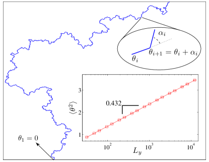
Figure 1: (color online) Defining $\alpha_{i}$ as the turning angle between two adjacent edges, $i$ and $i+1$, their winding angles $\theta_{i}$ and $\theta_{i+1}$ are related by $\theta_{i+1}=\theta_{i}+\alpha_{i}$, with $\theta_{1}=0$, as illustrated in the main figure. We performed simulations for 18 different lattice sizes, with $L_{y}=2^{4+n}$ and $3\times 2^{3+n}$ for $n=1,2,\dots,9$. Results are averages over $10^{6}$ samples for the smallest system sizes and $3\times 10^{3}$ for the largest one. Inset: Dependence of the variance of the winding angle on the lateral size of the lattice $L_{y}$. Statistical error bars are smaller than the symbols. The slope in the linear-log plot corresponds to $\kappa/4=0.432\pm 0.002$.

Winding angle. Using conformal invariance and Coulomb-gas techniques, Duplantier and Saleur Duplantier and Saleur (1988) have found the dependence of the distribution of the winding angle on the system size and the Coulomb-gas parameter. Given the correspondence of the Coulomb-gas parameter to $\kappa$, the relation for the winding angle can be extended to SLE Wieland and Wilson (2003). To analyze the winding angle $\theta_{i}$ at edge $i$, we set $\theta_{1}=0$ and define $\alpha_{i}$ as the turning angle between the edges $i$ and $i+1$ (see Fig. 1). The winding angle of each edge is then computed iteratively as $\theta_{i+1}=\theta_{i}+\alpha_{i}$. For SLE_κ, the variance of the winding angle over all edges in the curve scales as $\langle\theta^{2}\rangle=b+(\kappa/4)\ln L_{y}$, where $b$ is a constant and $L_{y}$ the lateral size of the lattice . Figure 1 shows the variance as function of lateral size $L_{y}$ for the WS, with a slope $0.432\pm 0.002$ in a linear-log plot. This slope corresponds to $\kappa=1.728\pm 0.008$ which is in good agreement with the one predicted by Eq. (1) from the WS fractal dimension.

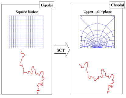
Figure 2: (color online) Original (left) and mapped (right) watershed. The Schwartz-Christoffel transformation (SCT) has been applied to map from the square lattice (left) to the upper half-plane (right). In this way dipolar curves are turned into chordal curves.

From dipolar to chordal representation. In the original setup, WS are dipolar curves which start at one point on the lower boundary and end when they touch the upper boundary, for the first time. For the left-passage probability and direct SLE evaluations, exact results are however known for chordal curves Schramm (2001), which start at the same point but go to infinity. Therefore, to proceed with these evaluations, we map the dipolar WS curves into chordal ones in the upper half-plane $\mathbb{H}$ (see Fig. 2). For such mapping, as suggested in Refs. Chatelain (2012); Driscoll (1996), we used the inverse Schwartz-Christoffel transformation .

Left-passage probability. For SLE curves in the upper half-plane $\mathbb{H}$, starting at the origin, the probability that a point $Re^{i\phi}$ is at the right side of the curve (see Fig. 3(a)) solely depends on $\phi$ and $\kappa$ and is given by Schramm’s formula Schramm (2001),

$$P_{\kappa}(\phi)=\frac{1}{2}+\frac{\Gamma\left(\frac{4}{\kappa}\right)}{\sqrt{\pi}\Gamma\left(\frac{8-\kappa}{2\kappa}\right)}\cot(\phi)_{2}F_{1}\left(\frac{1}{2};\frac{4}{\kappa},\frac{3}{2};-\cot^{2}(\phi)\right)\ \ ,$$ (2)

where ${}_{2}F_{1}$ is the Gaussian hypergeometric function and $\Gamma$ is the Gamma function. Figure 3(b) are the data points for the difference between the numerically measured probability $P(\phi,R)$ and the one predicted by Schramm’s formula, Eq. (2), for the chordal curve. It is shown that $P(\phi,R)$ is independent on $R$. To estimate $\kappa$ we plot, in Fig. 3(c), the mean square deviation $Q(\kappa)$ defined as,

$$Q(\kappa)=\frac{1}{M}\sum_{R}\sum_{\phi}\left[P(\phi,R)-P_{\kappa}(\phi)\right]^{2}\ \ ,$$ (3)

where the outer sum goes over values of $0.05\leq R\leq 1.2$, in steps of $0.05$, and the inner one over values of $0\leq\phi\leq\pi$, in steps of $\pi/15$. $M$ is the total number of considered points $Re^{i\phi}$. To reduce the statistical noise we used the relation $P(\phi,R)+P(\pi-\phi,R)=1$. The minimum in the plot corresponds to the value of $\kappa$ that best fits the left-passage probability, giving $\kappa=1.73\pm 0.01$, in line with the prediction based on the fractal dimension of WS, given by Eq. (1).

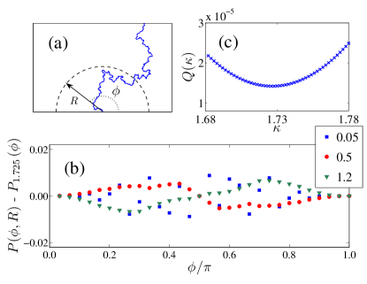
Figure 3: (color online) (a) Schematic representation of the left-passage definition (details in the text). (b) $P(\phi,R)-P_{1.725}(\phi)$ for the chordal watershed at different distances from the origin $R=\{0.05,0.5,1.2\}$, where $P_{1.725}(\phi)$ is the left-passage probability for $\kappa=1.725$ given by Schramm’s formula, Eq. (2). (c) Mean square difference $Q(\kappa)$ between the numerical data and Schramm’s formula (Eq. (3)) for different values of $\kappa$, exhibiting a minimum at $\kappa=1.73\pm 0.01$. In both cases, results are averages over $10^{5}$ curves on square lattices with $L_{y}=512$.

Direct SLE. Consider a chordal SLE curve $\gamma(t)$ which starts at a point on the real axis and grows to infinity inside the region of the upper half-plane $\mathbb{H}$, parametrized by an adimensional parameter $t$, typically called Loewner time. To compute its driving function $\xi(t)$ one needs to find the sequence of maps $g_{t}(z)$ which at each time $t$ map the upper half-plane $\mathbb{H}$ into $\mathbb{H}$ itself and satisfy the Loewner equation Löwner (1923). This map is unique and can be approximately obtained by considering the driving function to be constant within an interval $\delta t$, obtaining the slit map,

$$g_{t}(z)=\xi(t)+\sqrt{\left(z-\xi(t)\right)^{2}+4\delta t}\ \ ,$$ (4)

where $z$ is a point in $\mathbb{H}$ and $\delta t$ also depends on $t$. This map converges to the exact one for vanishing $\delta t$ Bauer and Bernard (2003). Initially, we set $t=0$ and $\xi(0)=0$ and we proceed iteratively through all points $z_{i}$ of the chordal curve. At each iteration $j$, we map the point $z_{j}$ to the real axis, by setting $\delta t_{j}=\left(\text{Im }z_{j}\right)^{2}/4$ and the driving function $\xi(t_{j})=\text{Re }z_{j}$ (being Re and Im the real and imaginary parts, respectively). We also compute the Loewner time $t_{j}=t_{j-1}+\delta t_{j}$. As referred above, in SLE, the driving function is related to a Brownian motion $B(t)$, with vanishing mean value and unit dispersion, such that $\xi(t)=\sqrt{\kappa}B(t)$ Schramm (2001).

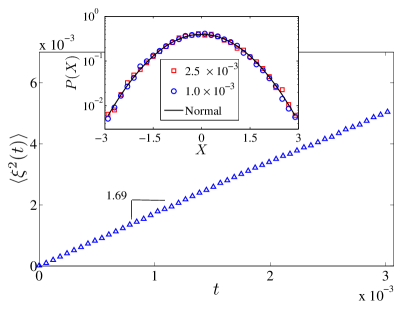
Figure 4: (color online) Dependence of the second moment of the driving function $\langle\xi^{2}(t)\rangle$ on the Loewner time, for the chordal watershed. The slope corresponds to $\kappa=1.69\pm 0.05$. Inset: Probability distribution of the driving function at two different Loewner times for chordal watersheds. The rescaled parameter $X$ is defined as $X=\xi(t)/\sqrt{\kappa t}$, where we have taken $\kappa=1.69$. The solid line is the normal distribution of vanishing mean value and unit dispersion. Results are averages over $4\times 10^{4}$ realizations on a square lattice with $L_{y}=1024$.

Figure 4 shows the second moment of the driving function for the chordal WS. The inset displays the probability distribution for the rescaled driving function $X=\xi(t)/\sqrt{\kappa t}$ for two different times for the chordal WS. All results are consistent with a Brownian motion with vanishing mean value and unit dispersion, when $\kappa=1.69\pm 0.05$, in good agreement with the results discussed above. The direct SLE analysis is characterized by larger error bars than the other two methods (winding angle and left-passage probability) due to strong discretization effects in the slit mapping Bauer and Bernard (2003).

Discussion. Our detailed numerical analysis shows that watersheds are likely to be SLE curves with $\kappa=1.734\pm 0.005$. This is the first documented case of a physical model with $\kappa<2$, lying outside the well-known duality conjecture range $2\leq\kappa\leq 8$, giving $\kappa^{\prime}=16/\kappa$, where $\kappa^{\prime}$ is the diffusivity of the dual model Dubédat (2005). It has been proven that SLE_κ with $\kappa>8$ is not reversible Zhan (2008), therefore if a dual model exists which respects reversibility, then it cannot be SLE${}_{\kappa^{\prime}}$ with ${\kappa^{\prime}}>8$. In the context of SLE, duality implies that two apparently different fractal dimensions might actually stem from the same curve. Geometrically, this corresponds to a relation between the fractal dimension of the accessible external perimeter and the one of the curve.

Our work shows that watersheds are non-local SLE curves. Although a connection with SLE is strong indication for conformal invariance, it cannot be interpreted as a proof. Nevertheless, if such invariance is established, it becomes possible to develop a field theory for this new universality class. CFT has helped to classify continuous critical behavior in two-dimensional equilibrium phenomena Di Francesco et al. (1997); Henkel and Karevski (2012). A well-established relation between diffusivity $\kappa$ and central charge $c$ of minimal CFT models which have a second level null vector in their Verma module is $c=(3\kappa-8)(6-\kappa)/2\kappa$ Bauer and Bernard (2003). If the watershed is conformally invariant it likely corresponds to a logarithmic CFT (LCFT) with central charge $c\approx-7/2$. A series of LCFT’s corresponding to loop models have been suggested in Ref. Provencher et al. (2012), which thus seem to be related to watersheds. It is also noteworthy that negative central charges have been reported in different contexts like, e.g., stochastic growth models, $2D$ turbulence, and quantum gravity Duplantier (1992); Flohr (1996); Lipatov (1999). In particular, the loop erased random walk is believed to have $\kappa=2$ which corresponds to $c=-2$. Besides, since the watershed of a landscape is based on the distribution of heights, the configurational space grows with $N!$, where $N$ is the number of sites, being a promising candidate to develop a field theory with quenched disorder.

The connection between SLE and statistical properties of the watershed opens up new possibilities. Since the latter are related to fractal curves emerging in several different contexts, our work paves the way to bridge between connectivity in disordered media and optimization problems where the same $\kappa$, and its corresponding central charge, are observed. Besides, a systematic study of the $\kappa$ dependence on correlations in the landscape might provide the required information to find SLE curves on natural landscapes. The possibility of a multifractal spectrum for watersheds is also an open question.