Excitonic and vibronic spectra of Frenkel excitons in a two-dimensional simple lattice

Abstract

Excitonic and vibronic spectra of Frenkel excitons (FEs) in a two-dimensional (2D) lattice with one molecule per unit cell have been studied and their manifestation in the linear absorption is simulated. We use the Green function formalism, the vibronic approach (see Lalov and Zhelyazkov [Phys. Rev. B 75, 245435 (2007)]), and the nearest-neighbor approximation to find expressions of the linear absorption lineshape in closed form (in terms of the elliptic integrals) for the following 2D models: (a) vibronic spectra of polyacenes (naphthalene, anthracene, tetracene); (b) vibronic spectra of a simple hexagonal lattice. The two 2D models include both linear and quadratic FE–phonon coupling. Our simulations concern the excitonic density of state (DOS), and also the position and lineshape of vibronic spectra (FE plus one phonon, FE plus two phonons). The positions of many-particle (MP-unbound) FE–phonon states, as well as the impact of the Van Hove singularities on the linear absorption have been established by using typical values of the excitonic and vibrational parameters. In the case of a simple hexagonal lattice the following types of FEs have been considered: (i) non-degenerate FEs whose transition dipole moment is perpendicular to the plane of the lattice, and (ii) degenerate FEs with transition dipole moments parallel to the layer. We found a cumulative impact of the linear and quadratic FE–phonon coupling on the positions of vibronic maxima in the case (ii), and a compensating impact in the case (i).

I Introduction

Frenkel excitons (FEs) and their vibronics have been studied for several decades. simpson57 ; davydov71 The theoretical basis of the vibronic studies and their connection with spectroscopic data have been established in papers, merrifield64 ; rashba66 ; philpott67 ; rashba68 ; philpott71 as well as in a couple of reviews and books. sheka72 ; broude85 ; agranovich09 The studies of charge transfer systems enlarge the applicability of the exciton theory towards the concept of charge transfer excitons (CTEs) and their vibronics. agranovich09 ; petelenz96 ; henessy99 ; hoffmann00 ; hoffmann02 ; lalov05 ; lalov06 The coupling between FE, CTEs, and phonons complicates the vibronic spectra manifesting themselves in various linear and nonlinear phenomena. Several mechanisms of this coupling combined with the intermolecular transfer of quasiparticles create bound (one-particle) exciton–phonon states and unbound many-particle (MP) states with rather different lineshapes. The models of vibronic spectra need productive methods of calculations and interpretation of the spectral pictures.

In this paper, we calculate the vibronic spectra of a two-dimensional (2D) lattice with one molecule per unit cell. Two types of symmetry of the molecules’ positions inside such a plane lattice are the subject of our study, notably

(a) Monoclinic or triclinic symmetry. This model mimics the ($a,b$)-plane of polyacenes. We use some crystallographic and spectroscopic data for the crystals of anthracene, tetracene, and naphthalene in our 2D models. The polyacene crystals exhibit layered structure which is better pronounced in the crystals of increasing number of the benzene rings. Our hypothesis of simple lattice neglects the effect of Davydov splitting (that effect has been treated, e.g., in the paper by Warns et al. warns11 and in Lalov et al. lalov11 ). The model of simple lattice allows us to obtain analytical and relatively simple results.

(b) Hexagonal symmetry. The 2D sheets of hexagonal symmetry are actual nowadays not only because of their connection to the study of graphene but also in the crystal engineering of layered hexagonal structures (see, e.g., Thalladi et al. thalladi95 ).

In the present paper we follow the vibronic approach developed and successfully applied in our previous papers, lalov07 ; lalov08a ; lalov08b in which one-dimensional models have been considered. Our present 2D study seems to be more realistic, especially for the case of polyacenes. The 2D models, however, limit the opportunity to treat the mixing of FE and CTEs. Whereas in 1D models this mixing can be described using three exciton branches (one of FE plus two of CTEs), the 2D models must include more than one decade of branches (see Petelenz et al., petelenz96 where the number of mixed exciton branches is 14). The intention to simulate the details of the vibronic spectra and to interpret their structure is the reason to limit ourselves with the model of vibronic spectra of FE only in the simple lattice with one molecule per unit cell. Moreover, according to nowadays concept the lowest singlet exciton in polyacenes is the Frenkel exciton and this is an argument for the treatment of FEs and their vibronics without mixing with CTEs.

In calculating the linear optical susceptibility, $\chi$, we use the formalism of the Green functions at $T=0$ and the nearest neighbor approximation. In this way, we express $\chi$ and calculate the linear absorption in terms of the complete elliptic integrals of the first kind

$$K(k)=\int_{0}^{\pi/2}\!\!\!\frac{d\phi}{\sqrt{1-k^{2}\sin^{2}\phi}}.$$ (1)

The outline of the paper is the following: in the second section we introduce the Hamiltonian and calculate the linear optical susceptibility in the range of one- and two-phonon vibronic spectra of a simple 2D lattice. In Sec. 3 those general expressions are specified for monoclinic and triclinic 2D lattices and using crystallographic and spectroscopic data for polyacenes we make simulations of their excitonic and vibronic spectra. Our calculations concern the vibronics of anthracene, tetracene, and naphthalene with intramolecular vibration at frequency of $1400$ cm^-1, but for the last crystal we simulate also the well studied vibronics with vibrations at frequency of $702$ cm^-1. Section 4 deals with the vibronics in a hexagonal 2D lattice with one molecule per unit cell. Two types of FEs are the subject of our studies of the excitonic density of states (DOS) and of linear absorption, namely (i) non-degenerate FEs whose transition dipole moment is perpendicular to the plane of the lattice, and (ii) degenerate FEs whose transition dipole moments are parallel to the layer. Section 5 summarizes our findings and contains some conclusions. In the Appendix, the Hamiltonian of degenerate FEs in the case of a hexagonal lattice is established to split into two fully identical Hamiltonians of left and right FEs.

II Hamiltonian and linear optical susceptibility in a simple 2D lattice

We consider the excitonic and vibronic excitations in a 2D lattice ($a,b$) with one molecule per unit cell. In the nearest neighbor approximation the FE part of the Hamiltonian reads

$${\hat{H}}_{\rm F}=\sum_{n}E_{\rm F}B^{+}_{n}B_{n}+\sum_{n,m}W_{nm}B^{+}_{n}B_{m},$$ (2)

where $B_{n}\,\left(B^{+}_{n}\right)$ is the operator of annihilation (creation) of the electronic excitation on the molecule $n$, $E_{\rm F}$ is the excitation energy of a molecule in the layers, and $W_{nm}$ is the transfer integral of FE between molecules $n$ and $m$. One mode of the intramolecular vibration at frequency $\omega_{0}$ is supposed to be coupled with the FE and $a_{n}$ is the annihilation operator of one vibrational quantum on the molecule $n$. Then the phonon part of the Hamiltonian can be written down as

$${\hat{H}}_{\rm ph}=\sum_{n}\hbar\omega_{0}a^{+}_{n}a_{n}.$$ (3)

We suppose both linear and quadratic FE–phonon coupling rashba66 ; philpott67 ; rashba68 with a Hamiltonian in the form

$${\hat{H}}_{\rm ex\text{--}ph}=\sum_{n}\xi\hbar\omega_{0}B^{+}_{n}B_{n}\left(a_{n}+a^{+}_{n}\right)$$

$${}+\sum_{n}\hbar\Delta\omega B^{+}_{n}B_{n}a^{+}_{n}a_{n},$$ (4)

where $\xi$ is a dimensionless parameter characterizing the linear FE–phonon coupling and $\Delta\omega$ is the change of the vibrational frequency of a molecule with electronic excitation on it (quadratic coupling). The three parts (2), (3), and (II) of the Hamiltonian can be transformed with the goal of eliminating the linear coupling by using the canonical transformation davydov71 ; rashba66

$${\hat{H}}_{1}=\exp(Q)\hat{H}\exp(-Q),$$ (5)

where

$$Q=\sum_{n}\xi B^{+}_{n}B_{n}\left(a_{n}^{+}-a_{n}\right).$$ (6)

In the transformed Hamiltonian the linear coupling terms are absent but the operators $B_{n}$ are replaced by

$$V_{n}=\exp(Q)B_{n}\exp(-Q)$$ (7)

(for more details see Lalov and Zhelyazkov lalov06 ). In the momentum space $(k_{a},k_{b})$ the operator (2) is transformed into

$${\hat{H}}_{\rm F}=\sum_{k_{a},k_{b}}\left[E_{\rm F}+W\left(k_{a},k_{b}\right)\right]V^{+}_{k_{a},k_{b}}V_{k_{a},k_{b}},$$ (8)

where the matrix element $W\left(k_{a},k_{b}\right)$ of the intermolecular transfer depends on the symmetry and on the strength of the intermolecular interaction.

We use the following formulas davydov71 ; agranovich09 in calculating the linear optical susceptibility

$$\chi_{ij}=\lim_{\varepsilon\to 0}\left\{-\frac{1}{2\hbar V}\left[\Phi_{ij}(\omega+i\varepsilon)+\Phi_{ij}(-\omega+i\varepsilon)\right]\right\}$$ (9)

with

$$\Phi_{ij}(t)=-i\theta(t)\langle 0|{\hat{P}}_{i}(t){\hat{P}}_{j}(0)+{\hat{P}}_{j}(t){\hat{P}}_{i}(0)|0\rangle,$$ (10)

where $V$ is the volume of the crystal (layer), and ${\hat{P}}$ is the operator of the transition dipole moment. The Green functions (10) have been calculated as an average over only the ground state $|0\rangle$ taking into account the large values of $E_{\rm F}$ and that $\hbar\omega_{0}\gg k_{\rm B}T$. In the expression of the operator ${\hat{P}}$ we preserve the transition moment of the FE only that reads

$${\hat{P}}_{\rm F}=\sum_{n}\mathbf{P}_{\rm F}\left(V_{n}+V^{+}_{n}\right).$$ (11)

Here $\mathbf{P}_{\rm F}$ is the transition dipole moment of the electronic excitation on the molecule $n$. The calculations of $\chi$ are reduced to calculating the following Green functions:

$$G_{n}^{(0)}(t)=-i\theta(t)\langle 0|V_{n}(t)V_{0}^{+}(0)|0\rangle.$$ (12)

In calculating their Fourier transforms in momentum space, $G^{(0)}(0,0)$, we obtain the following equation:

$$\left[\hbar\omega-E_{\rm F}-W(0,0)\right]G^{(0)}(0,0)=1+\hbar\omega_{a}S^{(1)},$$ (13)

where

$$\omega_{a}=\xi\omega_{1},\qquad\omega_{1}=\omega_{0}+\Delta\omega,$$ (14)

and $S^{(1)}$ is the sum on the whole 2D Brillouin zone $(k_{a},k_{b})$ of the Fourier transforms of following Green functions:

$$G_{n,m}^{(1)}(t)=-i\theta(t)\langle 0|a_{m}(t)V_{n}(t)V_{0}^{+}(0)|0\rangle.$$ (15)

In calculating the Green functions (15) we obtain functions $G^{(2)}$ with two phonon operators $\langle 0|a_{n}(t)a_{m}(t)V_{n}(t)\cdots$ and correspondingly one ladder with more complicated Green functions appears. Namely calculating them we use the vibronic approach lalov07 in which the transfer terms $W\left(k_{a},k_{b}\right)$ are taken in one step of the ladder only.

If we are interested in one-phonon vibronic spectra, the following equation of the component $G^{(1)}\left(k_{a},k_{b}\right)$ is valid

$$\left\{\hbar\left[\omega-\omega_{0}-\Omega_{r}(1)\right]-E_{\rm F}-W\left(k_{a},k_{b}\right)\right\}G^{(1)}\left(k_{a},k_{b}\right)=\hbar\omega_{a}G^{(0)}(0,0)+\alpha S^{(1)},$$ (16)

where

$$\alpha=\hbar\left[\Omega_{0,r}(2)-\Omega_{r}(1)+\Delta\omega\right],$$ (17)

and $\Omega_{0,r}(2)$ and $\Omega_{r}(1)$ are the following continuous fractions:

$$\Omega_{0,r}(2)=\cfrac{2\omega_{a}^{2}}{\omega-E_{\rm F}/\hbar-2\omega_{1}-\cfrac{3\omega_{a}^{2}}{\omega-E_{\rm F}/\hbar-3\omega_{1}-\cfrac{4\omega_{a}^{2}}{\cdots}}},$$ (18)

$$\Omega_{r}(1)=\cfrac{\omega_{a}^{2}}{\omega-E_{\rm F}/\hbar-2\omega_{0}-\Delta\omega-\cfrac{2\omega_{a}^{2}}{\omega-E_{\rm F}/\hbar-3\omega_{0}-2\Delta\omega-\cfrac{3\omega_{a}^{2}}{\cdots}}}$$ (19)

After some algebra we find the following expression of the Fourier transform $G^{(0)}(0,0)$:

$$G^{(0)}(0,0)=\cfrac{1}{\hbar\omega-E_{\rm F}-W(0,0)-\cfrac{\hbar\omega_{a}^{2}T_{1}}{1-\alpha T_{1}}},$$ (20)

where

$$T_{1}=\sum_{k_{a},k_{b}}\left\{\hbar\left[\omega-\omega_{0}-\Omega_{r}(1)\right]-E_{\rm F}-W\left(k_{a},k_{b}\right)\right\}^{-1}.$$ (21)

Finally we find the following expression of the linear optical susceptibility:

$$\chi_{xx}=-A\frac{P_{\rm F}^{2}}{v}G^{(0)}(0,0),$$ (22)

in which $A$ depends upon the units, $v$ is the volume occupied by one molecule, and the $x$-axis is directed along the direction of the transition dipole moment $\mathbf{P}_{\rm F}$. In the region of the two-phonon vibronic spectra the same procedure yields the expression lalov07

$$G^{(0)}(0,0)=\cfrac{1}{\hbar\omega-E_{\rm F}-W(0,0)-\cfrac{\hbar\omega_{a}^{2}}{\omega-E_{\rm F}/\hbar-\omega_{1}-\cfrac{2\omega_{a}^{2}T_{2}}{1-\alpha_{2}T_{2}}}},$$ (23)

where

$$\alpha_{2}=2\hbar\Delta\omega+\hbar\omega_{a}^{2}\left[\cfrac{3}{\omega-E_{\rm F}/\hbar-3\omega_{1}-\cfrac{4\omega_{a}^{2}}{\omega-E_{\rm F}/\hbar-4\omega_{1}-\cfrac{5\omega_{a}^{2}}{\cdots}}}-\Omega_{r}(2)\right],$$ (24)

$$\Omega_{r}(2)=\cfrac{\omega_{a}^{2}}{\omega-E_{\rm F}/\hbar-3\omega_{0}-\Delta\omega-\cfrac{2\omega_{a}^{2}}{\omega-E_{\rm F}/\hbar-4\omega_{0}-2\Delta\omega-\cfrac{3\omega_{a}^{2}}{\cdots}}},$$ (25)

and

$$T_{2}=\sum_{k_{a},k_{b}}\left\{\hbar\left[\omega-2\omega_{0}-\Omega_{r}(2)\right]-E_{\rm F}-W\left(k_{a},k_{b}\right)\right\}^{-1}.$$ (26)

III Two-dimensional lattice of monoclinic and triclinic symmetry

In this case, the molecules create a plane rhombohedral or rectangular network with two nearest neighbors at $a$-direction and other two nearest neighbors at $b$-direction. We denote by $W_{a}/2$ the transfer integral between the neighbors in the $a$-direction and by $W_{b}/2$ the transfer integral in the $b$-direction. The quantity $W\left(k_{a},k_{b}\right)$ can read as

$$W\left(k_{a},k_{b}\right)=W_{a}\cos\left(k_{a}a\right)+W_{b}\cos\left(k_{b}b\right),$$ (27)

and we find the following expressions of the quantity $T_{1}$ (and $T_{2}$ as well):

$$T_{1}=\frac{\sin\beta}{\pi\sqrt{|W_{a}W_{b}|}}I,$$ (28)

where $\beta$ is the angle between the $a^{*}$ and $b^{*}$ axes in the reciprocal space. To simplify notation we introduce also the following quantities:

$$\beta_{1}=\omega-E_{\rm F}/\hbar-\omega_{0}-\Omega_{r}(1)\quad\mbox{and}\quad\beta_{2}=\omega-E_{\rm F}/\hbar-2\omega_{0}-\Omega_{r}(2),$$ (29)

$$t=\left\{\begin{array}[]{cc}{\displaystyle\frac{\hbar\beta_{1}}{|W_{b}|}}\quad\mbox{for one-phonon vibronic},\\ {\displaystyle\frac{\hbar\beta_{2}}{|W_{b}|}}\quad\mbox{for two-phonon vibronic},\end{array}\right.$$ (30)

$$p=\left|\frac{W_{a}}{W_{b}}\right|,\quad k_{1}=\sqrt{\frac{4p}{t^{2}-(p-1)^{2}}},\quad k_{2}=\sqrt{\frac{(p+1)^{2}-t^{2}}{4p}}.$$ (31)

Then the integral $I$ in Eq. (28) can be calculated (assuming $|W_{b}|>|W_{a}|$) as follows:

$$I =-k_{1}K(k_{1})\quad\mbox{for}\quad\mathrm{Re}(t)<-1-p,$$ (32a)

$$I =-K(1/k_{1})-iK(k_{2})\quad\mbox{for}\quad-1-p<\mathrm{Re}(t)<-1+p,$$ (32b)

$$I =-\frac{i}{k_{2}}K(1/k_{2})\quad\mbox{for}\quad-1+p<\mathrm{Re}(t)<1-p,$$ (32c)

$$I =K(1/k_{1})-iK(k_{2})\quad\mbox{for}\quad 1-p<\mathrm{Re}(t)<1+p,$$ (32d)

$$I =k_{1}K(k_{1})\quad\mbox{for}\quad\mathrm{Re}(t)>1+p.$$ (32e)

The same expressions are valid for $T_{2}$ but with substituting $\beta_{2}$ for $\beta_{1}$.

We note here that the quantity $T_{1}$ expresses the excitonic density of states (DOS) at $\omega_{0}=0$, $\xi=0$, and $\Delta\omega=0$. Then we need the Fourier transform $G^{(0)}\left(k_{a},k_{b}\right)$ of the retarding Green function (12) which enters the expression of DOS, $\rho(\omega)$, in the excitonic band:

$$\rho(\omega)=-\pi\mathrm{Im}\sum_{k}G^{(0)}(k,\omega)\;\mbox{ at }\;\omega_{0}=0,\>\xi=0,\>\Delta\omega=0,\>\omega\to\omega+i\delta\;\mbox{ for }\delta\to 0.$$ (33)

Finally, it is easy to obtain the following relationship:

$$\rho(\omega)=-\pi\mathrm{Im}T_{1}(\omega_{0}=0,\xi=0,\Delta\omega=0)\quad\mbox{when}\quad\delta\to 0.$$ (34)

III.1 Simulations of excitonic DOS and vibronic spectra of 2D models of polyacenes

Naphthalene and anthracene crystals are of monoclinic symmetry and their crystallographic axes $a$ and $b$ are orthogonal as are $a^{*}$ and $b^{*}$ of their reciprocal lattices. Tetracene crystals are triclinic and the angle $\alpha_{0}$ between the $a$ and $b$ axes is approximately equal to $100^{\circ}$ but the $a^{*}$ and $b^{*}$ axes in the reciprocal lattice are almost perfectly orthogonal.

In the spectra of the three crystals we are largely interested in the intensive and widely studied electronic transition whose transition electric dipole moment $\mathbf{P}_{\rm F}$ is directed along the $M$-axis of the molecule I (see Campbell et al. campbell62 ). In our model we calculate the transition integrals $W_{a}$ and $W_{b}$ due to the nearest-neighbor dipole–dipole interaction of the equal dipole moments $\mathbf{P}_{\rm F}$ of each molecule of the 2D $(a,b)$-lattice. The distance between neighbor dipoles is taken to coincide with the lattice parameters $a$ and $b$.

Table 1 contains some crystallographic data of polyacenes crystals campbell62 ; schlosser80 which have been used in the simulations.

Table 1: Crystallographic data of polyacenes.campbell62

Crystal	Symmetry	$a$ (Å)	$b$ (Å)	$\alpha=(\widehat{a,b})$	$\psi_{M}$	$\chi_{M}$
Naphthalene	Monoclinic	8.24	6.00	90∘	29.5∘	$\approx\!\!69.6^{\circ}$
Anthracene	Monoclinic	8.56	6.04	90∘	26.6∘	71.3∘
Tetracene	Triclinic	7.90	6.03	100.3∘	30.1∘	69.2∘

Table 2 contains spectroscopic data necessary for our simulations. We take those data from Schlosser and Philpott schlosser80 ; schlosser82 to calculate the transfer integrals $W_{a}$ and $W_{b}$ as the nearest neighbor dipole–dipole interaction. Recall that in Table 2 $\mu=P_{\rm F}/e$ is the dipole transition moment measured in angstroms. In naphthalene the lowest excitonic

Table 2: Spectroscopic data for excitonic and vibronic spectra of polyacenes.schlosser80

Crystal	$E_{\rm F}$ (eV)	$\hbar\omega_{0}$ (eV)	$\mu=P_{\rm F}/e$ (Å)	$W_{a}$ (eV)	$W_{b}$ (eV)	$\xi^{2}$
Naphthalene I	4.33	0.1772	0.54	0.0097	$-0.049$	$1.67$
Naphthalene II	3.87	0.0942	0.104	$-1\times 10^{-5}$	$-0.011$	$0.4$
Anthracene	3.11	0.1735	0.61	0.012	$-0.068$	$0.9753$
Tetracene	2.615	0.1772	0.69	0.012	$-0.078$	$1.207$

transition is very weak (transition II in Table 2) with an oscillator strength of the polarization parallel to the $b$-axis, $f_{b}\approx 4\times 10^{-3}$, and respectively for polarization parallel to the $a$-axis, $f_{a}\approx 2\times 10^{-5}$ (see Chap. 2 in Broude et al. broude85 ). The calculated values of $W_{a}$ and $W_{b}$ are correspondingly much lower in comparison to other transfer integrals. The previous spectroscopic studies of molecular and crystal spectra exposed a significant shift, $\hbar\Delta\omega=-0.007$ eV, of the vibrational frequency in an excited molecule.

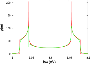
Figure 1: (Color online) Excitonic DOS in the case of dispersion (27) in the excitonic band. $E_{\rm F}=3.1$ eV, $W_{a}=0.012$ eV, $W_{b}=-0.068$ eV. The red curve is calculated at $\hbar\delta=0$, and the green one at $\hbar\delta=1\times 10^{-3}$ eV.

In the following we use relative units and suppose that the product $AP_{\rm F}^{2}/v\equiv 1$. We add an imaginary part, $i\delta$, to $\omega$ which expresses the excitonic damping and perform the calculations with $\hbar\delta=1\times 10^{-3}$ eV. The linear absorption coefficient is calculated as imaginary part of the component $\chi_{bb}$ (for electromagnetic waves of polarization parallel to the $b$-axis)

$$\chi_{bb}=-\cos^{2}\psi_{M}\,G^{(0)}(0,0).$$ (35)

The excitonic DOS calculated by using formula (33) is shown in Fig. 1. The well-known Van Hove singularities hove53 for the case of 2D models are exhibited. The function of DOS has non-zero values at the edges of the excitonic band and it manifests two singular points of logarithmic behavior. The final excitonic damping (the green curve) preserves the course of DOS but it makes the singularities softer.

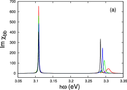
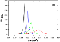
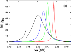
Figure 2: (Color online) Vibronic spectra of the anthracene 2D model. The excitonic peak is fitted at $E_{\rm F}=3.11$ eV, $W_{a}=0.012$ eV, $W_{b}=-0.068$ eV. The red curve is calculated at $\xi^{2}=0.6$, the green at $\xi^{2}=0.8$, the blue at $\xi^{2}=0.9753$, and the black at $\xi^{2}=1.2$, all curves for $\Delta\omega=0$ and $\hbar\omega_{0}=0.1735$ eV. Clip (a): general picture of the excitonic peak and the absorption curves of one-phonon vibronics (formula (20)). Clip (b): absorption curves near $E_{\rm F}+\hbar\omega_{0}$ (the first replica). Clip (c): absorption curves near $E_{\rm F}+2\hbar\omega_{0}$ (second vibronics, formula (23)).

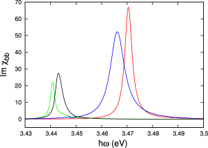
Figure 3: (Color online) Two-phonon vibronic spectra of the anthracene 2D model. The red curve has been calculated for $\xi^{2}=0.8$, $\hbar\Delta\omega=0$; green curve for $\xi^{2}=0.8$, $\hbar\Delta\omega=-0.01$ eV; blue curve for $\xi^{2}=0.9735$, $\hbar\Delta\omega=0$; and the black curve for $\xi^{2}=0.9735$, $\hbar\Delta\omega=-0.01$ eV.

The linear absorption simulations of the anthracene 2D model calculated on using formulas (20) and (23) yield the curves in

Figure 4: Linear absorption spectra of the naphthalene I model. $E_{\rm F}=4.33$ eV; $\hbar\omega_{0}=0.1772$ eV; $\xi^{2}=1.67$; $\Delta\omega=0$; $W_{a}=0.0097$ eV, and $W_{b}=-0.049$ eV. Clip (a): general picture of the vibronic series calculated on using formula (20). Clip (b): absorption curves near $E_{\rm F}+\hbar\omega_{0}$. Clip (c): absorption curves near $E_{\rm F}+2\hbar\omega_{0}$, calculated by means of formula (23).

Fig. 2. In our calculations, the value of $E_{\rm F}$ is a free parameter (see Ref. lalov07, ) and it is fitted to obtain the excitonic peak at $3.11$ eV. For small values of the linear exciton–phonon coupling (red and green curves) the absorption curves in Fig. 2(b) are wide and correspond to the many-particle (MP) states. The half-width of the black curve is approximately of $1\times 10^{-3}$ eV and it is Lorentzian which corresponds to the bound (one-particle) exciton–phonon state. The blue curve is calculated for values of $\xi$ close to the widely used values of anthracene and it corresponds to a quasi-bound state inside the MP band near its minimum. The jumps in the absorption curves are associated with the singular points of DOS.

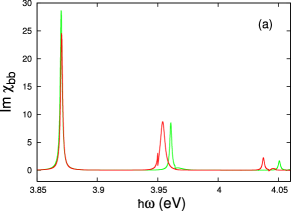
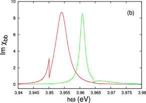
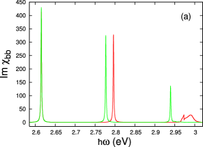
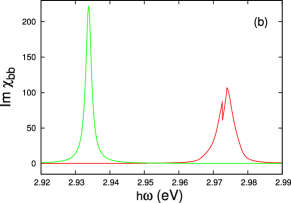
Figure 5: (Color online) Linear absorption of the lowest excitonic peak and its vibronic replica of naphthalene II (see Table 2). $E_{\rm F}=3.87$ eV; $\hbar\omega_{0}=0.0942$ eV; $\xi^{2}=0.4$; $\hbar\Delta\omega=-0.0072$ eV. The green curve has been calculated for $W_{b}=-0.011$ eV, $W_{a}=-1\times 10^{-5}$ eV; for red curve $W_{b}=0.011$ eV, $W_{a}=1\times 10^{-5}$ eV. Clip (a): general picture. Clip (b): the region of the first vibronic spectra $E_{\rm F}+\hbar\omega_{0}$. A factor of $0.04$ decreases the values of the absorption in comparison to Fig. 4.

Figure 6: (Color online) Linear absorption of the tetracene 2D model. $E_{\rm F}=2.615$ eV; $\hbar\omega_{0}=0.1772$ eV; $\xi^{2}=1.207$; $W_{a}=0.012$ eV, $W_{b}=-0.0781$ eV. The red curve corresponds to $\Delta\omega=0$, and the green curve to $\hbar\Delta\omega=-0.02$ eV. Clip (a): absorption curves calculated by using formula (20). Clip (b): absorption curves near $E_{\rm F}+2\hbar\omega_{0}$ calculated with the help of formula (23).

All curves in Fig. 2(c), calculated for the second vibronics $E_{\rm F}+2\hbar\omega_{0}$, exhibit behavior of MP states. The position of the MP bands can be found using the same formulas (20) and (23) but at $\delta=0$. In this case, one-particle states do not manifest themselves in the linear absorption spectra but MP bands appear due to the imaginary parts in formulas (32). The calculations at $\delta=0$ show that even the most narrow band for $\xi^{2}=0.6$ is positioned inside the MP band. It is curious to note the inverse situation in vibronic spectra with two phonons compared to Fig. 2(b). The increasing linear excitation makes the absorption curves wider (in one-phonon vibronic spectra it binds the FE and phonon), however, shifts them in the region of lower frequencies like curves in Fig. 2(b). The impact of the quadratic exciton–phonon coupling expressed by $\Delta\omega$ is more pronounced in the two-phonon vibronic region (see Fig. 3). The shift of the absorption curves to lower frequencies is even more than $2\hbar\Delta\omega$ (compare red and green curves, blue and black curves) but the quadratic coupling transfers intensities from two-phonon vibronic to one-phonon vibronic spectra.

The vibronic series of the naphthalene I model (see Table 2) is shown in Fig. 4. Obviously the first vibronic replica (look at Fig. 4(b)) is dominated by the strong one-particle maximum accompanied by a relatively weak MP band in the region $4.505$–$4.53$ eV. The situation near the second vibronic (see Fig. 4(c)) is very similar, however, the one-particle maximum and the MP band have comparable absorption intensities.

The excitonic maximum, $E_{\rm F}=3.87$ eV, and its vibronic replica have been intensively investigated davydov71 ; sheka72 ; broude85 despite of their weak intensities. Our simulations shown in Fig. 6 confirm the results obtained by using an 1D model (see Ref. lalov07, ). In the case of negative values of the transfer integrals $W_{a}$ and $W_{b}$ the absorption spectrum consists of one-particle maximum and a very weak MP band (green curve in Fig. 6). In the case of positive transfer integrals (red curve) the linear absorption demonstrates the transfer of unbound FE and phonon.

The linear absorption of the tetracene 2D model presented in Fig. 6 exhibits one-particle maximum near $E_{\rm F}+\hbar\omega_{0}$ and a MP band near the second vibronic replica. In polyacenes, the vibration of quantum $\hbar\omega_{0}\approx 0.17$ eV is an example of presumably linear FE–phonon coupling and thus the red curves in Fig. 6 are more realistic. The hypothetical strong quadratic coupling causes the binding of FE and phonons and one-particle states only occur in the linear absorption.

IV Two-dimensional lattice of hexagonal symmetry

Each molecule in a plane hexagonal lattice with one molecule per unit cell is surrounded by six neighbors spaced at a distance $a$. We us the unit cell with vectors $\mathbf{a}$ and $\mathbf{b}$ of displacement from molecule $0$ to molecules $1$ and $2$ and the angle $\alpha_{0}$ between $\mathbf{a}$ and $\mathbf{b}$ is $60^{\circ}$ ($|\mathbf{a}|=|\mathbf{b}|=a$). The angle $\beta$ between the $a^{*}$ and $b^{*}$ axes of reciprocal space is equal to $120^{\circ}$.

Two types of FEs will be considered in the following text: (i) non-degenerate FEs of transition dipole moment perpendicular to the plane of the hexagonal layer, and (ii) degenerate FEs whose transition dipole moments are parallel to the layer.

The transfer integral $V_{1}$ between the molecule $0$ and its six nearest neighbors can be calculated using the formula for the potential energy of two molecular transition dipole moments $\mathbf{p}_{1}$ and $\mathbf{p}_{2}$ whose centers are spaced by a vector $\mathbf{r}$

$$W=\frac{(\mathbf{p}_{1}\cdot\mathbf{p}_{2})\,r^{2}-3\,(\mathbf{p}_{1}\cdot\mathbf{r})(\mathbf{p}_{1}\cdot\mathbf{r})}{4\pi\varepsilon_{0}r^{5}},$$ (36)

where $\varepsilon_{0}=8.8542\times 10^{-12}$ F m^-1 is the electric constant.

In the case of non-degenerate FEs the transition dipole moments $|\mathbf{p}_{1}|=|\mathbf{p}_{2}|=p$ are perpendicular to the vector $\mathbf{r}$ and we obtain

$$V_{1}=\frac{p^{2}}{4\pi\varepsilon_{0}a^{3}}>0\qquad(|\mathbf{r}|=a).$$ (37)

In the case of degenerate FEs their transition dipole moments directed along the perpendicular axes $x$ and $y$ inside the plane of the layers are equal: $h_{x}=h_{y}=h$ (see the Appendix). Using the same formula (36) one obtains the transfer integrals of both left and right FEs

$$V_{1}=-\frac{h^{2}}{8\pi\varepsilon_{0}a^{3}}<0.$$ (38)

Irrespective of the different signs of the transfer integrals $V_{1}$ of non-degenerate and degenerate FEs one obtains

$$W\left(k_{a},k_{b}\right)=2V_{1}\left\{\cos(\gamma k_{a})+\cos(\gamma k_{b})+\cos\left[\gamma\left(k_{a}+k_{b}\right)\right]\right\},$$ (39)

where $\gamma=a\sqrt{3}/2$. We introduce the quantities

$$s=\frac{\hbar\beta_{1}}{2V_{1}},\qquad d=\sqrt{3-2s},$$ (40)

$$k_{1}=\sqrt{\frac{4d}{s^{2}-3+2d}},\qquad k_{2}=\sqrt{\frac{4d}{3-s^{2}+2d}}.$$ (41)

Then the sums $T_{1}$ and $T_{2}$ (see formulas (21) and (26)) can be expressed using the integral $I$:

$$T_{1}=\frac{\sqrt{3}}{2\pi V_{1}}I,$$ (42)

whose new values now are given by

$$I =\frac{k_{1}}{2\sqrt{d}}K(k_{1})\quad\mbox{for}\quad\mathrm{Re}(s)<-3,$$ (43a)

$$I =\frac{1}{2\sqrt{d}}\left[K(1/k_{1})-i\,\text{sgn}(V_{1})K(1/k_{2})\right]\quad\mbox{for}\quad-3<\mathrm{Re}(s)<1,$$ (43b)

$$I =-\frac{k_{2}}{2\sqrt{d}}\left[2K\left(\sqrt{\frac{3-s^{2}-2d}{3-s^{2}+2d}}\right)+i\,\text{sgn}(V_{1})K(k_{2})\right]\quad\mbox{for}\quad 1<\mathrm{Re}(s)<3/2,$$ (43c)

$$I =-\frac{2}{\sqrt[4]{(s-1)^{3}(s+3)}}K\left(\sqrt{\frac{1}{2}\left(1-\frac{s^{2}-3}{\sqrt{(s-1)^{3}(s+3)}}\right)}\right)\quad\mbox{for}\quad\mathrm{Re}(s)>3/2.$$ (43d)

The excitonic DOS in the case of excitonic dispersion (39) can be calculated with the help of formula (34). In the simulations of DOS and linear optical absorption we put the excitonic vibrational parameters typical for organic solids, more specifically

$$\hbar\omega_{0}=0.17\mbox{ eV},$$

$$\xi^{2}=0.64,\quad\mbox{or}\quad 1,\quad\mbox{or}\quad 1.44,$$

$$\hbar\Delta\omega=0\qquad\mbox{or}\qquad-0.01\mbox{ eV}.$$

In estimating the transfer integral $V_{1}$ we suppose a dipole–dipole approximation between two transition dipoles $p$ (or $h/\sqrt{2}$) $=3$ D situated at a distance $a=8\times 10^{-10}$ m. Then the calculations of their potential energy give (approximately)

(a) $V_{1}=0.011$ eV for non-degenerate FEs. We fit the excitonic level at $E_{\rm F}=3.27$ eV.

(b) $V_{1}=-0.011$ eV for degenerate FEs with $E_{\rm F}=3.06$ eV.

The excitonic DOS in the case of dispersion low (39) is presented in Fig. 7. Only one saddle point that corresponds to

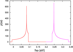
Figure 7: (Color online) Excitonic DOS in the case of dispersion described by formula (39). For non-degenerate FEs $E_{\rm F}=3.27$ eV, $V_{1}=0.011$ eV, while for degenerate FEs $E_{\rm F}=3.06$ eV and $V_{1}=-0.011$ eV.

$\mathrm{Re}(s)=1$ (see formulas (40)–(43)) exists in the excitonic band. In the center of the Brillouin zone, $k_{a}=k_{b}=0$, the values of DOS at $\mathrm{Re}(s)=-3$ are relatively low.

IV.1 The case of degenerate Frenkel excitons ($\bm{V_{1}}\bm{<}\bm{0}$)

In Fig. 8(a) one sees the calculated absorption curves near the excitonic peak and one-phonon vibronic spectra. In Fig. 8(b) are shown the lowest parts of the same dispersion curves calculated at $\delta=0$ (no excitonic damping) in the bands of the many-particle FE–phonon states.

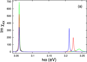
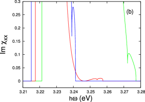
Figure 8: (Color online) Linear absorption in a simple hexagonal 2D lattice for $E_{\rm F}=3.06$ eV, $\hbar\Delta\omega=0.17$ eV, $\hbar\Delta\omega=0$, $V_{1}=-0.011$ eV. The green curve has been calculated at $\xi=0.8$, the red for $\xi=1$, and the blue for $\xi=1.2$. Clip (a): excitonic peak ant its vibronic replicas at $\hbar\delta=1\times 10^{-3}$ eV. Clip (b): Details of the absorption curves in the MP bands at $\delta=0$.

We emphasize again that the absorption at $\delta=0$ manifests itself in the MP bands only. The points of a sharp change in the three absorption curves correspond to the singular point $\mathrm{Re}(s)=1$. Both panels of Fig. 8 show that the green curve for $\xi=0.8$ describes absorption in the MP band, the red curve ($\xi=1$) corresponds to a quasi-one particle state above the minimum of the MP band while the blue curve ($\xi=1.2$) describes one-particle (bound) FE–phonon state below the MP band.

The impact of the quadratic FE–phonon coupling ($\hbar\delta\neq 0$) on the absorption curves is clearly seen in Fig. 9. The absorption

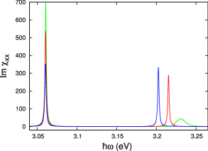
Figure 9: (Color online) Linear absorption as in Fig. 8 but for $\hbar\Delta\omega=-0.01$ eV.

maxima are shifted approximately at $\hbar\Delta\omega$ below their positions in Fig. 8(a) and the maximum of the red curve ($\xi=1$) describes also a one-particle state.

Figure 10 illustrates the absorption near the second vibronic replica $E_{\rm F}+2\hbar\omega_{0}$. The linear FE–phonon coupling is

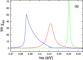
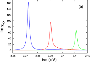
Figure 10: (Color online) Linear absorption as in Fig. 8 near the second replica, $E_{\rm F}+2\hbar\omega_{0}$. Clip (a): the case $\hbar\Delta\omega=0$. Clip (b): the case $\hbar\Delta\omega=-0.01$ eV.

not sufficient to bind the FE and two phonons and the three absorption curves in Fig. 10(a) describe MP states. The calculations performed at $\delta=0$, similar to those in Fig. 8(b), confirm the position of the maximum on the green curve inside the MP band irrespective of its narrow width. The quadratic coupling shifts the two-phonon vibronic maxima in the direction of lower energy—see Fig. 10(b). Unlike the case of linear coupling (look at Fig. 10(a)) the maximum of the blue curve ($\xi=1.2$) corresponds to bound states while the maximum of the red curve ($\xi=1$) is associated with a quasi-bound state.

Our studies of the linear absorption show that both coupling mechanisms decrease the frequencies of the absorption maxima of the degenerate FE–phonon states ($V_{1}<0$).

IV.2 The case of non-degenerate Frenkel excitons ($\bm{V_{1}}\bm{>}\bm{0}$)

The picture of the absorption curves at $V_{1}>0$ seems to be a little surprising (see Fig. 11). The absorption maxima appear near

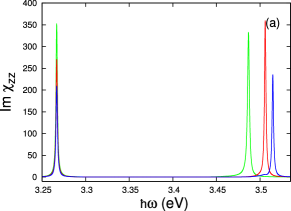
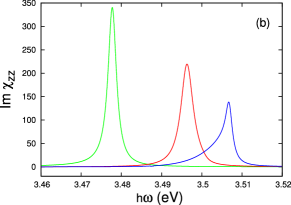
Figure 11: (Color online) Linear absorption in a 2D model of hexagonal lattice—the case of non-degenerate FEs—excitonic peak and first vibronic spectra. Here $E_{\rm F}=3.27$ eV, $\hbar\omega_{0}=0.17$ eV, $\hbar\delta=1\times 10^{-3}$ eV, $V_{1}=0.011$ eV. The green curves have been calculated at $\xi=0.8$, the red curves for $\xi=1$, and blue ones for $\xi=1.2$. Clip (a): the case $\Delta\omega=0$. Clip (b): the case $\hbar\Delta\omega=-0.01$ eV.

the maximum of the MP band (green curve) and even above the PM bands (red and blue curves). The distance between the excitonic peak ($E_{\rm F}=3.27$ eV) and one-phonon vibronic maxima is bigger than $\hbar\omega_{0}=0.17$ eV. Hence, the linear FE–phonon coupling at $V_{1}>0$ repulses the vibronic levels and increases their energy. In contrast, the quadratic coupling (see Fig. 11(b)) decreases the values of the vibronic levels and one-particle bound states above the MP bands in Fig. 11(a) are transformed into unbound states inside the MP bands (red and blue curves in Fig. 11(b)).

The three absorption curves in Fig. 12 correspond to the MP bands.

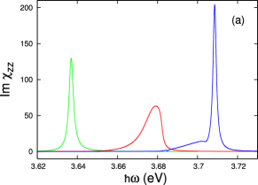
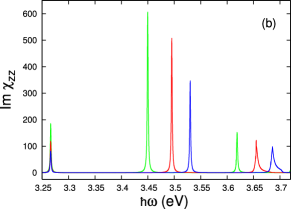
Figure 12: (Color online) Linear absorption spectra as in Fig. 11 near the second vibronic replica, $E_{\rm F}+2\hbar\omega_{0}$, calculated by means of formula (23). Clip (a): the case $\hbar\Delta\omega=0$. Clip (b): the case $\hbar\Delta\omega=-0.01$ eV.

The absorption at $\xi=1.2$ (blue curve) exhibits also the existence of one-particle state—see the high maximum above the energy of $3.705$ eV in Fig. 12(a). Like the one-phonon vibronic spectra (see Fig. 11) the simultaneous action of the linear and the quadratic couplings (look at Fig. 12(b)) shifts in opposite directions the two-phonon vibronic spectra. We stress on the difference between absorption curves in Fig. 11(b) (calculated by using expression (20)) and the absorption in the same region $3.45$–$3.50$ eV in Fig. 12(b) (calculated with the help of formula (23)). Formula (20) concerns one-phonon vibronic spectra (see Fig. 11) and is not valid for the one-phonon maxima calculated using the expression (23) that describes the two-phonon vibronic spectra.

The most interesting result of our 2D model in the case of a FE polarized perpendicularly to the layer is the opposite action of the two coupling mechanisms on the position of the vibronic maxima.

V Conclusion

In the present paper, we investigate the excitonic and vibronic spectra of FEs manifesting themselves in 2D plane lattices with one molecule per unit cell of the following types: (i) monoclinic or triclinic lattice which mimics the $(a,b)$ plane of polyacenes, and (ii) simple hexagonal lattice. We study the exciton dispersion and the excitonic DOS in the nearest neighbor approximation as well as calculate the linear optical susceptibility and the linear absorption spectra in the range of a FE and its vibronics with one and two quanta of intramolecular vibration coupled with the FE by linear and quadratic couplings. The model of a lattice with one molecule per unit cell yields relatively simple expressions with complete elliptic integrals of the first kind. Our approach allows us to find the positions of the MP (unbound) FE–phonon bands and of the one-particle (bound) states outside those bands. The Van Hove singularities appear in the DOS of the 2D models and they affect the linear absorption spectra.

In the case of a hexagonal 2D lattice our studies concern two types of dipole-active FEs: (i) non-degenerate FEs of transition dipole moment perpendicular to the layer and of positive transfer integral, $W$; (ii) degenerate FEs of transition dipole moments parallel to the layer and of negative transfer integrals. In the last case, we establish a splitting of the Hamiltonian into two fully identical Hamiltonians which do not mix in the dipole approximation and describe two types of FEs of different hiralities (left and right, respectively). The simulations of the vibronic spectra exhibit a opposite impact of the linear FE–phonon coupling on the positions of the vibronic maxima: in case (i) of non-degenerate FEs it repulses those maxima to the upper boundary of the MP bands or above these bands. In case (ii) of degenerate FEs the linear coupling decreases the energy of the vibronic maxima. Since the quadratic coupling in the usual case of $\hbar\Delta\omega<0$ decreases this energy, the simultaneous action of both coupling mechanisms can have a cumulative effect in case (ii) or a compensating one in case (i).

The 2D simulations of the vibronic spectra of naphthalene and anthracene in the present paper agree well with the 1D simulation in Ref. lalov07, , however, new peculiarities in the absorption near the singular points could appear. Especially inside the two-phonon MP bands narrow vibronic maxima can be observed even at small values of the linear coupling constant $\xi$ (see Figs. 2(c), 10(a), and 12(b)).

The intriguing models of layered polyacenes and of graphene, both with two molecules per unit cell can not be described using the relatively simple expressions of the present paper—one needs the usage of elliptic integrals of the third kind for an adequate modeling. Nevertheless, many conclusions for the absorption inside and outside the MP bands are still valid. The studies of the excitonic dispersion and the structure of the vibronic spectra can be useful in the modeling of the excitonic transfer and the exciton–phonon coupling manifesting themselves in other linear and nonlinear phenomena.

*

Appendix A Hamiltonian of degenerate Frenkel excitons

The dipole-active FEs whose transition dipole moments are parallel to the hexagonal layer are two-fold degenerate. The same two-fold degenerate electronic excitations must exist in each molecule of the monolayer. In the lack of rotational symmetry of molecules in the ($x,y$)-plane of the monolayer it is impossible to ensure optical isotropy inside that plane.

We choose the axes $x$ and $y$ to be perpendicular to each other and parallel to the monolayer. The Hamiltonian and the transition dipole moment of each molecule contain the following components:

$$\hat{H}_{\rm mol}=E_{\rm F}\left(B^{+}_{x}B_{x}+B^{+}_{y}B_{y}\right),$$ (44)

$$\hat{P}_{\rm mol}=h\left[\left(B^{+}_{x}+B_{x}\right)\hat{x}+\left(B^{+}_{y}+B_{y}\right)\hat{y}\right],$$ (45)

where $B_{x}$ and $B_{y}$ are the operators of annihilation of the electronic excitations in a molecule with transition dipole moment directed along the $x$/$y$-axis, and $\hat{x}$ and $\hat{y}$ are the corresponding unit vectors. We introduce the following operators:

$$\begin{split}B^{+}_{l}=\left(B^{+}_{x}+iB^{+}_{y}\right)/\sqrt{2},\;B_{l}=\left(B_{x}-iB_{y}\right)/\sqrt{2},\\ B^{+}_{r}=\left(B^{+}_{x}-iB^{+}_{y}\right)/\sqrt{2},\;B_{r}=\left(B_{x}+iB_{y}\right)/\sqrt{2}.\end{split}$$ (46)

The usual boson commutation rules are valid for the operators (46). Thus, operators (44) and (45) take the forms

$$\hat{H}_{\rm mol}=E_{\rm F}\left(B^{+}_{l}B_{l}+B^{+}_{r}B_{r}\right),$$ (47)

$$\hat{P}_{\rm mol}=(h/\sqrt{2})\left[(\hat{x}-i\hat{y})\left(B^{+}_{l}+B_{r}\right)\right.$$

$$\left.{}+(\hat{x}+i\hat{y})\left(B^{+}_{r}+B_{l}\right)\right].$$ (48)

The point group of symmetry of the hexagonal plane monolayer can be $C_{6}$, $C_{3h}$, or $D_{6h}$ depending on the symmetry of the molecules. In all cases the two-dimensional $(x,y)$-representation of the point group can be presented by the following two one-dimensional representations whose direct product is a totally symmetrical unit-representation: (i) left ($l$) with molecular transition dipole moment $(h/\sqrt{2})(\hat{x}-i\hat{y})$, and (ii) right ($r$) with transition dipole moment $(h/\sqrt{2})(\hat{x}+i\hat{y})$.

The non-vanishing terms in the crystal Hamiltonian must be invariant for all operations of symmetry of the crystal and the binary terms of the energy operator and that of the intermolecular interaction must be a product of the two different representations, $r$ and $l$, respectively. In the Heitler-London approximation (see Davydov davydov71 and Agranovch agranovich09 ) we neglect the terms

$$\left(B^{+}_{r,n}B^{+}_{l,m}+\mbox{h.c.}\right)$$

and the only non-vanishing transfer terms are of the type

$$\left(B^{+}_{r,n}B_{r,m}+B^{+}_{l,n}B_{l,m}\right).$$

In dipole–dipole approximation the corresponding transfer integral $V_{1}$ can be calculated using formula (39) for the two dipoles

$$\mathbf{p}_{1}=(h/\sqrt{2})(\hat{x}-i\hat{y})\qquad\mbox{and}\qquad\mathbf{p}_{2}=(h/\sqrt{2})(\hat{x}+i\hat{y}).$$

In this way, one obtains formula (38). The transfer integrals, $V_{1}$, for the excitations $l$ and $r$ are equal and the excitonic Hamiltonian, as well as operator (II) of the exciton–phonon coupling, split into two independent parts $l$ and $r$ which do not mix, notably

$$\hat{H}_{\rm F}=\sum_{l,r}\left[\sum_{n}E_{\rm F}B^{+}_{(l,r);n}B_{(l,r);n}\right.$$

$$\left.{}+\sum_{m,n}V_{mn}B^{+}_{(l,r);m}B_{(l,r);n}\right].$$ (49)

Hence, the Hamiltonian $\hat{H}_{1}$ can be divided into two independent Hamiltonians $\hat{H}_{1,l}$ and $\hat{H}_{1,r}$ fully analogous to Eq. (8). In calculating the linear optical susceptibility, $\chi$, we apply the approach used in Sec. II for the transition dipole moment (A). Since FEs of type $r$ and $l$ do not mix, the non-vanishing Green functions of the type (12) in the Hamiltonian must have equal chirality $r$ or $l$ of the operators $V(t)$ and $V^{+}(0)$. The final expression for the components

$$\chi_{xx}=\chi_{yy}$$ (50)

is fully identical to (22) but with $h$ instead of $P_{\rm F}$ and new values of the transfer integrals $V_{1}$ which are negative—compare expressions (37) and (38).

References

- (1) W. T. Simpson and D. L. Peterson, J. Chem. Phys. 26, 588 (1957).
- (2) A. S. Davydov, Theory of Molecular Excitons (Plenum Press, New York, 1971).
- (3) R. E. Merrifield, J. Chem. Phys. 40, 445 (1964).
- (4) E. I. Rashba, Sov. Phys. JETF 23, 708 (1966).
- (5) M. R. Philpott, J. Chem. Phys. 47, 2534 (1967).
- (6) E. I. Rashba, Sov. Phys. JETF 27, 292 (1968).
- (7) M. R. Philpott, J. Chem. Phys. 55, 2039 (1971).
- (8) E. F. Sheka, Sov. Phys. Usp. 14, 484 (1972).
- (9) V. L. Broude, E. I. Rashba, and E. F. Sheka, Spectroscopy of Molecular Excitons (Springer, Berlin, 1985).
- (10) V. M. Agranovich, Excitations in Organic Solids (Oxford University Press, New York, 2009).
- (11) P. Petelenz, M. Slawik, K. Yokoi, and M. Z. Zgierski, J. Chem. Phys. 105, 4427 (1996).
- (12) M. H. Henessy, Z. G. Soos, R. A. Pascal Jr., and A. Girlando, Chem. Phys. 245,199 (1999).
- (13) M. Hoffmann, K. Schmidt, T. Fritz, T. Hasche, V. M. Agranovich, and K. Leo, Chem. Phys. 258, 73 (2000).
- (14) M. Hoffmann and Z. G. Soos, Phys. Rev. B 66, 024305 (2002).
- (15) I. J. Lalov, C. Supritz, and P. Reineker, Chem. Phys. 309, 189 (2005).
- (16) I. J. Lalov and I. Zhelyazkov, Phys. Rev. B 74, 035403 (2006).
- (17) C. Warns, I. Lalov, and P. Reineker, Phys. Procedia 13, 33 (2011), Selected Papers from 17th International Conference on Dynamical Processes in Excited States of Solids (DPC’10).
- (18) I. J. Lalov, T. Hartmann, and P. Reineker—submitted.
- (19) V. R. Thalladi, K. Panneerselvam, C. J. Carrell, H. L. Carrell, and G. R. Desiraju, J. Chem. Soc., Chem. Commun. issue 3, 341 (1995), DOI: 10.1039/C39950000341.
- (20) I. J. Lalov and I. Zhelyazkov, Phys. Rev. B 75, 245435 (2007).
- (21) I. J. Lalov, C. Supritz, and P. Reineker, Chem. Phys. 352, 1 (2008).
- (22) I. J. Lalov, C. Warns, and P. Reineker, New J. Phys. 10, 085006 (2008).
- (23) R. B. Campbell, J. M. Robertson, and J. Trotter, Acta Cryst. 15, 289 (1962).
- (24) D. W. Schlosser and M. R. Philpott, Chem. Phys. 49, 181 (1980).
- (25) D. W. Schlosser and M. R. Philpott, J. Chem. Phys. 77, 1969 (1982).
- (26) L. Van Hove, Phys. Rev. 89, 1189 (1953).