Soft-collinear resummation in deeply virtual Compton scattering

Abstract

We derive an all order resummation formula for the deeply virtual Compton scattering (DVCS) amplitude, which takes into account soft gluon exchanges in the non-singlet quark coefficient function. We identify the ladder diagrams responsible in light-like gauge for $(\alpha_{s}\log^{2}(x\pm\xi))^{n}$ contributions. The resummed series results in a simple closed expression.

In the collinear factorization framework the scattering amplitude for exclusive processes such as DVCS has been shown historyofDVCS to factorize in specific kinematical regions, provided a large scale controls the separation of short distance dominated partonic subprocesses and long distance hadronic matrix elements, the generalized parton distributions (GPDs) review . The amplitude for the DVCS process

$$\gamma^{(*)}(q)N(p)\to\gamma(q^{\prime})N^{\prime}(p^{\prime})\,.$$ (1)

with a large virtuality $q^{2}=-Q^{2}$, factorizes in terms of perturbatively calculable coefficient functions $C(x,\xi,\alpha_{s})$ and GPDs $F(x,\xi,t)$, where the scaling variable in the generalized Bjorken limit is the skewness $\xi$ defined as

$$\xi=\frac{Q^{2}}{(p+p^{\prime})\cdot(q+q^{\prime})}\,.$$ (2)

Lessons from the DVCS amplitude at NLO.

Let us begin with the discussion of the NLO corrections to the amplitude for DVCS (1). After proper renormalization, the quark contribution to the symmetric part of the factorized Compton scattering amplitude reads

$$\mathcal{A}^{\mu\nu}=g_{T}^{\mu\nu}\int_{-1}^{1}dx\left[\sum_{q}^{n_{F}}T^{q}(x)F^{q}(x)\right]\,,$$ (3)

where the quark coefficient function $T^{q}$ reads Pire:2011st

$$\!\!\!\!\!\!T^{q} \!\!= \!\!C_{0}^{q}+C_{1}^{q}+C_{coll}^{q}\log\frac{|Q^{2}|}{\mu^{2}_{F}}\,,$$ (4)

$$\!\!\!\!\!\!C_{0}^{q} \!\!= \!\!e_{q}^{2}\left(\frac{1}{x-\xi+i\varepsilon}\,-\,(x\to-x)\right)\,,$$ (5)

$$\!\!\!\!\!\!C_{1}^{q} \!\!= \!\!\frac{e_{q}^{2}\alpha_{S}C_{F}}{4\pi(x-\xi+i\varepsilon)}\bigg{\{}\log^{2}(\frac{\xi-x}{2\xi}-i\varepsilon)\,-\,9$$ (6)

$$-\,3\frac{\xi-x}{\xi+x}\log\bigg{(}\frac{\xi-x}{2\xi}-i\epsilon\bigg{)}\bigg{\}}-(x\to-x)\,.$$

The first (resp. second) terms in Eqs.  (5) and (6) correspond to the $s-$channel (resp. $u-$channel) class of diagrams. One goes from the $s-$channel to the $u-$channel by the interchange of the photon attachments. Since these two contributions are obtained from one another by a simple ($x\leftrightarrow-x$) interchange, we will restrict in the following mostly to the discussion of the former class of diagrams.

Eqs.  (5) and (6) show that among the corrections of $O(\alpha_{s})$ to the coefficient function, the terms of order $\frac{\log^{2}(x\pm\xi)}{x\pm\xi}$ play an important role in the region of small $(x\pm\xi)$, i.e. in the vicinity of the boundary between the so-called ERBL and DGLAP domains, where the evolution equations of GPDs take distinct forms.

Main steps of our analysis.

We start our analysis with the observation that in the same spirit as for evolution equations, the extraction of the soft-collinear singularities which dominate the amplitude in the limit $x\to\pm\xi$ is made easier if one uses the light-like gauge $p_{1}\equiv p_{\gamma}$. We argue that in this gauge the amplitude is dominated by ladder-like diagrams, see Fig. 1. In our analysis we expand any momentum in the Sudakov basis $p_{1}$, $p_{2}$, as $k=\alpha\,p_{1}+\beta\,p_{2}+k_{\perp}\,,$ where $p_{2}$ is the light-cone direction of the two incoming and outgoing partons ($p_{1}^{2}=p_{2}^{2}=0$, $2p_{1}\cdot p_{2}=s=Q^{2}/2\xi$). In this basis, $q_{\gamma^{*}}=p_{1}-2\,\xi\,p_{2}$ .

We now restrict our study to the limit $x\to+\xi$. The dominant kinematics is given by a strong ordering both in longitudinal and transverse momenta, according to

$$x\sim\xi\gg|\beta_{1}|\sim|x-\xi|\gg|x-\xi-\beta_{1}|\sim|\beta_{2}|\gg\cdots$$

$$\cdots\gg|x-\xi-\beta_{1}-\beta_{2}-\cdots-\beta_{n-1}|\sim|\beta_{n}|,$$ (7)

$$|k_{\perp 1}^{2}|\ll|k_{\perp 2}^{2}|\ll\cdots\ll|k_{\perp n}^{2}|\ll s\sim Q^{2}\,,$$ (8)

$$|\alpha_{1}|\ll\cdots\ll|\alpha_{n}|\ll 1\,.$$ (9)

This ordering is related to the fact that the dominant double logarithmic contribution for each loop arises from the region of phase space where both soft and collinear singularities manifest themselves. When $x\to\xi$ the left fermionic line is a hard line, from which the gluons are emitted in an eikonal way, with a collinear ordering. For the right fermionic line, eikonal approximation is not valid, since the dominant momentum flow along $p_{2}$ is from gluon to fermion, nevertheless the collinear approximation can still be applied.

Finally, the issue related to the $i\epsilon$ prescription in Eq. (6) is solved by computing the coefficient function in the unphysical region $\xi>1$. After analytical continuation to the physical region $0\leq\xi\leq 1$, the final result is then obtained through the shift $\xi\to\xi-i\epsilon$ .

To prepare for further analysis, we define $K_{n}$, the contribution of a $n$-loop ladder to the coefficient function, as

$$K_{n}=-\frac{i}{4}e_{q}^{2}\left(-i\,C_{F}\,\alpha_{s}\frac{1}{(2\pi)^{2}}\right)^{n}I_{n}\,.$$ (10)

Now we will discuss in details the main points of derivation of $I_{n}$ starting from the simplest case.

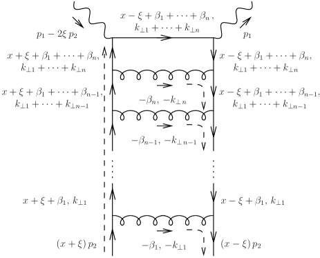
Figure 1: The ladder diagrams which contribute in the light-like gauge to the leading $\alpha_{s}^{n}\ln^{2n}(\xi-x)/(x-\xi)$ terms in the perturbative expansion of the DVCS amplitude. The $p_{2}$ and $\perp$ momentum components are indicated. The dashed lines show the dominant momentum flows along the $p_{2}$ direction.

The ladder diagram at order $\alpha_{s}$.

A careful analysis shows that the one-loop diagrams of Fig. 2 are not dominant for $x\to\xi\,$. Thus, we concentrate on the box diagram, see Fig. 1 with $n=1$. Starting from the dominant part of the numerator of the Born term which is $\not{\theta}=-2\not{p}_{1}$, the numerator of the box diagram is

$$tr\big{\{}\not{p_{2}}\gamma^{\mu}[\not{k}+(x-\xi)\not{p_{2}}]\not{\theta}[\not{k}+(x+\xi)\not{p_{2}}]\gamma^{\nu}\big{\}}d^{\mu\nu}\,.$$ (11)

We first perform the soft gluon approximation : $k+(x+\xi)p_{2}\to(x+\xi)p_{2}$. Since the gluon is almost on-shell, the dominant contribution in the gluon propagator, $d^{\mu\nu}$, when expressed in terms of gluon polarization vectors, is given by $d^{\mu\nu}\approx-\sum_{\lambda}\epsilon^{\mu}_{(\lambda)}\epsilon^{\nu}_{(\lambda)}\,.$ Writing gluon polarization vectors through their Sudakov decomposition

$$\epsilon^{\mu}_{(\lambda)}=\epsilon^{\mu}_{\perp(\lambda)}-2\frac{\epsilon_{\perp(\lambda)}\cdot k_{\perp}}{\beta s}p_{1}^{\mu}\,,$$ (12)

allows us to define an effective vertex for the gluon and outgoing quark through the polarization sum

$$\sum_{\lambda}\epsilon_{\perp(\lambda)}\cdot k_{\perp}\epsilon^{\mu}_{(\lambda)}=\bigg{(}-k_{\perp}^{\mu}+2\frac{k_{\perp}^{2}}{\beta s}p_{1}^{\mu}\bigg{)}\,.$$ (13)

The numerator, $(Num)_{1}$, is $\alpha-$independent and reads

$$\frac{-4(x+\xi)}{\beta}tr\bigg{\{}\!\!\not{p_{2}}\bigg{(}\not{k_{\perp}}-2\frac{k_{\perp}^{2}}{\beta s}\not{p_{1}}\bigg{)}[\not{k}+(x-\xi)\not{p_{2}}]\not{p_{1}}\!\!\bigg{\}}$$ (14)

$$= -4(x+\xi)s\frac{2k_{\perp}^{2}}{\beta}\bigg{[}1+\frac{2(x-\xi)}{\beta}\bigg{]}\,.$$

We emphasize that the term $(x+\xi)/\beta$ arises from the eikonal emission from the left fermionic line while the expression inside the $[\,\cdots]$ accounts for the fact that gluon is not soft from the point of view of the right fermion (in an eikonal treatment it would reduce to $(x-\xi)/\beta$).

Figure 2: The one-loop diagrams which do not contribute to the leading $\frac{\log^{2}(x-\xi)}{x-\xi}$ terms in the $p_{1}\cdot A=0$ light-like gauge.

Let us now calculate the integral over the gluon momentum $k$, using dimensional regularization $\int d^{d}k\rightarrow\frac{s}{2}\int d\alpha\,d\beta\,d^{d-2}\underline{k}$, $(k_{\perp}^{2}=-\underline{k}^{2})$. The Cauchy integration over $\alpha$, which also determines the limits of the $\beta$ integration, gives

$$I_{1} =-2\pi i\frac{s}{2}\bigg{\{}\int_{0}^{\xi-x}\frac{d\beta}{s\beta}\int_{0}^{\infty}d^{d-2}\underline{k}\frac{(Num)_{1}}{L_{1}^{2}\,R_{1}^{2}\,S^{2}}\Big{|}_{\alpha=\frac{\underline{k}^{2}}{\beta s}}$$ (15)

$$+ \int_{-\xi-x}^{\xi-x}\frac{d\beta}{s\beta}\int_{0}^{\infty}d^{d-2}\underline{k}\frac{(Num)_{1}}{L_{1}^{2}\,R_{1}^{2}\,S^{2}}\Big{|}_{\alpha=\frac{\underline{k}^{2}}{(\beta+x+\xi)s}}\bigg{\}}\,,$$

with the denominators of propagators $L_{1}$($R_{1}$) on the left (right) quark line and $S$ for s-channel quark line

$$L_{1}^{2} = \alpha(x+\xi)s~{}~{}~{},~{}~{}~{}R_{1}^{2}=-\underline{k}^{2}+\alpha(\beta+x-\xi)s\,,$$

$$S^{2} = -\underline{k}^{2}+(\beta+x-\xi)s\,.$$ (16)

It turns out that the first line in Eq. (15), which corresponds to cutting through the exchanged gluon, dominates. Moreover, the relevant region of integration corresponds to small $|\beta+x-\xi|$. The $\beta$ and $\underline{k}$ integrations results in our final one-loop expression

$$I_{1}=-\frac{4}{x-\xi}\frac{2\pi i}{2!}\log^{2}(a(x-\xi))\,,$$ (17)

where we kept only the most singular terms in the $x\to\xi$ region and have no control of the value of $a$ within our approximation. To fix $a$, we match our approximated one-loop result with the full one-loop result (6). This amounts to cut the $\underline{k}^{2}$ integral at $Q^{2}$. The $i\epsilon$ term is included according to the same matching. This leads to

$$I_{1}=-\frac{4}{x-\xi+i\epsilon}\frac{2\pi i}{2!}\log^{2}\left(\frac{\xi-x}{2\xi}-i\epsilon\right)\,.$$ (18)

A similar expression holds for the $u-$channel diagram in the limit $x\to-\xi\,.$

The ladder diagram at order $\alpha_{s}^{2}$.

Let us examine the next order in the perturbative expansion. There are many diagrams contributing but it can be shown that in the chosen gauge, the double box diagram dominates, and moreover that the relevant region of integration is where there is a strong ordering between $k_{2\perp}$ and $k_{1\perp}$, i.e. $k_{2\perp}\gg k_{1\perp}$. Using the same arguments as in the one-loop case, one simplifies the numerator for this diagram, after taking advantage of strong $k_{i\perp}$ ordering, as

$$(Num)_{2} = -4s(x+\xi)^{2}\bigg{\{}\frac{2k_{\perp 1}^{2}}{\beta_{1}}\bigg{[}1+\frac{2(x-\xi)}{\beta_{1}}\bigg{]}\bigg{\}}$$ (19)

$$\times\bigg{\{}\frac{2k_{\perp 2}^{2}}{\beta_{2}}\bigg{[}1+\frac{2(\beta_{1}+x-\xi)}{\beta_{2}}\bigg{]}\bigg{\}}\,.$$

The denominators of fermionic propagators read (Fig. 1)

$$L_{1}^{2} = \alpha_{1}(x+\xi)s~{}~{},~{}~{}R_{1}^{2}=-\underline{k}^{2}+\alpha_{1}(\beta_{1}+x-\xi)s\,,$$

$$L_{2}^{2} = \alpha_{2}(x+\xi)s~{}~{},~{}~{}R_{2}^{2}=-\underline{k}^{2}+\alpha_{2}(\beta_{1}+\beta_{2}+x-\xi)s\,,$$

$$S^{2} = -\underline{k}^{2}+(\beta_{1}+\beta_{2}+x-\xi)s\,.$$ (20)

Using Cauchy integration over $\alpha_{1}$ and $\alpha_{2}$, we see that the dominant contribution comes from the residues corresponding to the two gluon propagators, and reads

$$I_{2}\approx\int_{0}^{\xi-x}d\beta_{1}\int_{0}^{\xi-x-\beta_{1}}d\beta_{2}\int_{0}^{\infty}d^{d-2}\underline{k}_{2}\int_{0}^{\underline{k}_{2}^{2}}d^{d-2}\underline{k}_{1}\,{\cal I}_{2}\,,$$ (21)

where

$${\cal I}_{2}\!\!=\!\!\frac{4\,s(2\pi i)^{2}}{x-\xi}\frac{1}{\beta_{1}+x-\xi}\frac{1}{\underline{k}_{1}^{2}}\frac{1}{\underline{k}_{2}^{2}}\frac{1}{\underline{k}_{2}^{2}-(\beta_{1}+\beta_{2}+x-\xi)s}.$$ (22)

The integrals over $\underline{k}_{1}$ and $\underline{k}_{2}$ are performed by assuming that the singularities are regularized within dimensional regularization. Taking into account the fact that a scaleless integral vanishes, we get the following formula

$$I_{2}\approx-\frac{4}{x-\xi+i\epsilon}\frac{(2i\pi)^{2}}{4!}\log^{4}\left(\frac{\xi-x}{2\xi}-i\epsilon\right)\,.$$ (23)

The $i\epsilon$ and the $2\xi$ factor in the argument of the logarithm are fixed by hand, extending the matching used at the one-loop level. These prescriptions are not needed for the resummation of $[\alpha_{s}\log^{2}(\frac{\xi-x}{2\xi}-i\epsilon)]^{n}$ terms which we want to exhibit and are beyond the accuracy of our estimate.

The ladder diagram at order $\alpha_{s}^{n}$.

We now turn to the estimation of all $log^{2n}(x-\xi)$ terms. We again assume the strong ordering (8, 9) in $k_{\perp}$ and $\alpha$. The distribution of the poles generates nested integrals in $\beta_{i}$

$$\int_{0}^{\xi-x}d\beta_{1}\int_{0}^{\xi-x-\beta_{1}}d\beta_{2}\cdots\int_{0}^{\xi-x-\beta_{1}-\cdots-\beta_{n-1}}d\beta_{n}\,.$$ (24)

The simplified numerator for the $n^{th}$ order box diagram is obtained by generalizing the argument for the two-loop case. One gets

$$(Num)_{n}=-4s(x+\xi)^{n}\frac{2k_{\perp 1}^{2}}{\beta_{1}}\bigg{[}1+\frac{2(x-\xi)}{\beta_{1}}\bigg{]}\frac{2k_{\perp 2}^{2}}{\beta_{2}}$$ (25)

$$\bigg{[}1\!+\!\frac{2(\beta_{1}+x-\xi)}{\beta_{2}}\bigg{]}\!\!\cdots\!\frac{2k_{\perp n}^{2}}{\beta_{n}}\!\bigg{[}1\!+\!\frac{2(\beta_{n-1}+\!\cdots\!+\!\beta_{1}\!+\!x\!-\!\xi)}{\beta_{n}}\bigg{]}\!,$$

and the denominators of propagators are, for $i=1\cdots n$,

$$L_{i}^{2} = \alpha_{i}(x+\xi)s$$

$$R_{i}^{2} = -\underline{k}_{i}^{2}+\alpha_{i}(\beta_{1}+\cdots+\beta_{i}+x-\xi)s\,,$$

$$S^{2} = -\underline{k}_{i}^{2}+(\beta_{1}+\cdots+\beta_{i}+x-\xi)s\,.$$ (26)

Using dimensional regularization and omitting scaleless integrals, the integral $I_{n}$ reads

$$I_{n}=\int_{0}^{\xi-x}d\beta_{1}\cdots\int_{0}^{\xi-x-\cdots-\beta_{n-1}}d\beta_{n}\int_{0}^{\infty}d^{d-2}\underline{k}_{n}\cdots\int_{0}^{\underline{k}_{2}^{2}}d^{d-2}\underline{k}_{1}\,{\cal{I}}_{n}\,,\,\,$$ (27)

where

$${\cal{I}}_{n}\!\!=\!\!(-1)^{n}\frac{4\,s(2\pi i)^{n}}{x-\xi}\frac{1}{\beta_{1}+x-\xi}\cdots\frac{1}{\beta_{1}\!+\!\cdots+\!\beta_{n-1}\!+\!x\!-\!\xi}$$

$$\times\frac{1}{\underline{k}_{1}^{2}}\cdots\frac{1}{\underline{k}_{n}^{2}}\frac{1}{\underline{k}_{n}^{2}-(\beta_{1}+\cdots+\beta_{n}+x-\xi)s}\,.$$ (28)

The integrals over $\underline{k}_{1}\cdots\underline{k}_{n}$ are performed again in a similar way as in the case of one- and two-loops, resulting in

$$I_{n}=-\frac{4}{x-\xi+i\epsilon}\frac{(2\pi i)^{n}}{(2n)!}\log^{2n}\left(\frac{\xi-x}{2\xi}-i\epsilon\right)\,,$$ (29)

where the matching condition introduced in one-loop case is extended to $n-$loops.

The resummed formula.

Based on the results Eqs. (18, 23, 29), one can discuss the resummed formula for the complete amplitude. By combining Eq. (29) with Eq. (10), we get

$$\sum_{n=0}^{\infty}K_{n}=\frac{e_{q}^{2}}{x-\xi+i\epsilon}\cosh\left[D\log\left(\frac{\xi-x}{2\xi}-i\epsilon\right)\right]$$ (30)

$$=\frac{1}{2}\frac{e_{q}^{2}}{x-\xi+i\epsilon}\left[\left(\frac{\xi-x}{2\xi}-i\epsilon\right)^{D}+\left(\frac{\xi-x}{2\xi}-i\epsilon\right)^{-D}\right]\,.$$

Although the matching condition introduced at one-loop still does not fix the form of the resummed formula uniquely, since it requires to go beyond double logarithmic accuracy, it is natural to propose the following two forms

$$(C_{0}+C_{1})^{res}_{1}=\frac{e_{q}^{2}}{x-\xi+i\epsilon}\bigg{\{}\cosh\bigg{[}D\log\bigg{(}\frac{\xi-x}{2\xi}-i\epsilon\bigg{)}\bigg{]}$$

$$-\frac{D^{2}}{2}\bigg{[}9+3\frac{\xi-x}{x+\xi}\log\bigg{(}\frac{\xi-x}{2\xi}-i\epsilon\bigg{)}\bigg{]}\bigg{\}}-(x\rightarrow-x)\,,$$ (31)

with $D=\sqrt{\frac{\alpha_{s}C_{F}}{2\pi}}$ and

$$(C_{0}+C_{1})^{res}_{2}\!=\!\frac{e_{q}^{2}}{x-\xi+i\epsilon}\cosh\bigg{[}D\log\bigg{(}\frac{\xi-x}{2\xi}\!-\!i\epsilon\bigg{)}\bigg{]}$$ (32)

$$\times\bigg{\{}\!1-\frac{D^{2}}{2}\bigg{[}9+3\frac{\xi-x}{x+\xi}\log\bigg{(}\frac{\xi-x}{2\xi}-i\epsilon\bigg{)}\!\bigg{]}\!\bigg{\}}-(x\rightarrow-x)\,.$$

These resummed formulas differ through logarithmic contributions which are beyond the precision of our study.

Phenomenological perspectives.

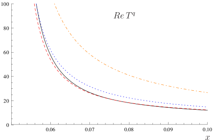
Figure 3: $Re\,T^{q}$ as a function of $x$, for $\xi=0.05$ and $\mu_{F}=Q$: coefficient function at LO (dot dashed-orange) and NLO (solid-black), resummed formulas (31) (dashed-red) and (32) (dotted-blue). For simplicity, $e_{q}=1\,.$

In Figs. 3 and 4 we show the real and imaginary parts of the resummed coefficient function ($\xi=0.05$ and $\alpha_{s}=0.33$, corresponding to $Q=2$ GeV and $\Lambda_{QCD}=.2$ GeV) together with the LO and NLO result, restricted to the DGLAP region. While the NLO corrections have sizable effects with respect to LO, Fig. 3 shows that the higher order corrections when resummed in our way do not dramatically lead to any further change of the coefficient function. This hints to a stabilized perturbative expansion around $x=\pm\xi\,.$ Nevertheless, Figs. 3 and 4 quantifies the sizable effects from the ambiguous choice of resummation formula (31, 32), demanding a higher order analysis.

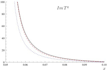
Figure 4: $Im\,T^{q}$ as a function of $x$, for $\xi=0.05$ and $\mu_{F}=Q$: NLO coefficient function (solid-black), resummed formulas (31) (dashed-red) and (32) (dotted-blue), with $e_{q}=1\,.$

Conclusions.

We have demonstrated that resummation of soft-collinear gluon radiation effects can be performed in hard exclusive reactions amplitudes. The resulting formula for coefficient function exhibits a different behaviour than both the Born order and the NLO results. A detailed investigation of the effect of resummation on observables such as the magnitude of Compton form factors will be performed elsewhere. A related but somewhat different expression should emerge in various hard exclusive reactions, such as exclusive meson electroproduction. The simplest extension of our formula will address the crossed case of timelike Compton scattering MPSW .

We did not study neither the effects of the running of $\alpha_{s}$ nor the case of gluon GPD contributions which, although they begin at order $\alpha_{s}$ are expected to be important in the small $\xi$ regime to be accessible at high energies EIC-LHeC . It has been customary to perform resummation in terms of Mellin moments papers-resummation . In our case, conformal Mellin moments may be more appropriate, and we will address this question in future work.

We thank A. H. Mueller, G. Sterman, O. V. Teryaev, J. Wagner, for useful discussions and correspondence. This work is partly supported by the Polish Grant NCN No DEC-2011/01/D/ST2/02069, the French-Polish collaboration agreement Polonium, the P2IO consortium and the Joint Research Activity ”Study of Strongly Interacting Matter” (acronym HadronPhysics3, Grant Agreement n.283286) under the Seventh Framework Programme of the European Community.

References

• (1) D. Müller et al., Fortsch. Phys.  42, 101 (1994); A. V. Radyushkin, Phys. Lett. B 380, 417 (1996); X. D. Ji and J. Osborne, Phys. Rev.  D 58, 094018 (1998) and Phys. Rev.  D 57, 1337 (1998); J. Collins and A. Freund, Phys. Rev.  D59, 074009 (1999).
• (2) K. Goeke, M. V. Polyakov and M. Vanderhaeghen, Prog. Part. Nucl. Phys.  47, 401 (2001); M. Diehl, Phys. Rept.  388, 41 (2003); A. V. Belitsky and A. V. Radyushkin, Phys. Rept.  418, 1 (2005).
• (3) A. V. Belitsky and D. Mueller, Phys. Lett. B 417, 129 (1998); A. V. Belitsky, D. Mueller, L. Niedermeier and A. Schafer, Phys. Lett. B 474, 163 (2000); B. Pire, L. Szymanowski and J. Wagner, Phys. Rev. D 83, 034009 (2011).
• (4) D. Mueller, B. Pire, L. Szymanowski and J. Wagner, arXiv:1203.4392 [hep-ph].
• (5) D. Boer et al., arXiv:1108.1713 [nucl-th]; O. Bruening et al., arXiv:1206.2913 [phys.acc-ph]; B. Pire, L. Szymanowski and J. Wagner, Phys. Rev. D 79 (2009) 014010.
• (6) A. Bassetto, M. Ciafaloni, G. Marchesini and A. H. Mueller, Nucl. Phys. B 207, 189 (1982); G. F. Sterman, Nucl. Phys. B 281, 310 (1987); S. Catani and L. Trentadue, Nucl. Phys. B 327, 323 (1989).