Nearshore wave forecasting and hindcasting by dynamical and statistical downscaling

Abstract

A high-resolution nested WAM/SWAN wave model suite aimed at rapidly establishing nearshore wave forecasts as well as a climatology and return values of the local wave conditions with Rapid Enviromental Assessment (REA) in mind is described. The system is targeted at regions where local wave growth and partial exposure to complex open-ocean wave conditions makes diagnostic wave modelling difficult.

SWAN is set up on 500 m resolution and is nested in a 10 km version of WAM. A model integration of more than one year is carried out to map the spatial distribution of the wave field. The model correlates well with wave buoy observations (0.96) but overestimates the wave height somewhat (18%, bias 0.29 m).

To estimate wave height return values a much longer time series is required and running SWAN for such a period is unrealistic in a REA setting. Instead we establish a direction-dependent transfer function between an already existing coarse open-ocean hindcast dataset and the high-resolution nested SWAN model. Return values are estimated using ensemble estimates of two different extreme-value distributions based on the full 52 years of statistically downscaled hindcast data. We find good agreement between downscaled wave height and wave buoy observations. The cost of generating the statistically downscaled hindcast time series is negligible and can be redone for arbitrary locations within the SWAN domain, although the sectors must be carefully chosen for each new location.

The method is found to be well suited to rapidly providing detailed wave forecasts as well as hindcasts and return values estimates of partly sheltered coastal regions.

Subject keywords: rapid environmental assessment, nearshore wave forecasting, wave hindcasting, statistical downscaling, dynamical downscaling, wave height return values.
Regional terms: Europe, Norway. North Sea.

1 Introduction

Coastal regions partially sheltered from the open ocean prove a difficult middle ground between open-ocean conditions and the really small scales found in harbours and the mouths of rivers and estuaries. Prognostic wave models developed for open-ocean conditions (see e.g. Hasselmann et al., 1988; Tolman, 1991) have until recently been considered too computer-intensive to be operated on grids resolving complex coastal regions (typically requiring a grid finer than 1 km).

In partially sheltered domains where local wave growth is limited and the ocean spectrum outside sheltering islands can be assumed spatially homogeneous it may be possible to use simple refraction-diffraction models O’Reilly and Guza (1993), especially if the main concern is relatively uni-directional low-frequency swell from distant storms. In such cases it may be possible to establish a tractable database (look-up table) of relations between open-ocean and nearshore conditions for various combinations of integrated parameters like significant wave height, peak direction and peak period of the wave field impinging on the boundary of the model domain. On even finer scale semi-diagnostic models designed for harbours, closed bays and estuaries (e.g. STWAVE, Smith et al., 2001) perform very well.

However, for coastal domains where local wave growth is of significance the steady-state assumption breaks down. Also, the complexity of the sea state near the open ocean with swell intrusion and young wind sea requires full two-dimensional spectra as boundary conditions to the fine-scale model. This is difficult to achieve with steady-state models because the aforementioned look-up table will grow out of bounds (the “curse of dimensionality”), making a fully non-stationary dynamical spectral wave model a computationally competitive alternative.

The advent of high-resolution prognostic wave models specifically designed to handle the high resolution needed to resolve nearshore conditions combined with numerical weather prediction models (NWP) capable of capturing the complexity of the coastal wind field opens up the possibility of forecasting the sea state in regions partly sheltered from the open ocean on spatial resolution of less than 1 km. Simulating WAves Nearshore (SWAN) is a third-generation wave model (Booij et al., 1999; Ris et al., 1999) in operational use at the Norwegian Meteorological Institute since 2006. The model is operated on 500 m resolution and is used to issue wave forecasts to the Norwegian Coastal Administration and the general public for particularly sensitive sea areas.

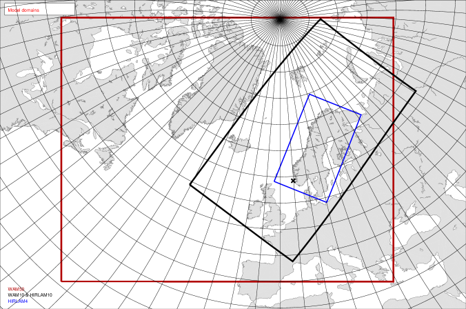
Figure 1: The model domains of the operational models used for providing boundary conditions for the SWAN dynamical downscaling during the 16-month period. The numerical weather prediction model HIRLAM4 covers Scandinavia and only the eastern part of the Norwegian Sea (blue). HIRLAM10 and the wave model WAM10 share the same domain and grid resolution (black) while WAM50 covers a large part of the North Atlantic to ensure that swell is properly accounted for (red). The location of the high-resolution SWAN model shown in Fig. 2 is marked with “x”. $5^{\circ}$ graticule, rotated plate carrée projection.

For this study SWAN was set up for a region on the west coast of Norway which is partially sheltered by islands to the north-west and with a larger island to the east, see Figures 1 and 2. We define a semi-sheltered coastal region as one that is exposed to wind and waves from the open ocean and is large enough for local wave growth to become important while still being sheltered by islands or mainland in other directions.

Running a high-resolution forecast system with SWAN as the wave component is computationally demanding, but tractable, in forecast mode. If detailed wind fields are also required (depending on the steepness of the topography), a detailed numerical weather prediction model must also be operated. In our case very detailed (4-5 km resolution) winds were used to force the wave model. The wind fields are taken from a high-resolution nested weather prediction system. Full two-dimensional wave spectra from a coarser wave model (WAM) are used as boundary conditions for the high-resolution model. This nested setup with full two-dimensional wave spectral information on the open boundaries will be referred to as the dynamical downscaling. Dynamical downscaling techniques for waves resemble the nesting methods employed for atmospheric and oceanographic modelling but with the important difference that the wave field is a forced dynamical system that depends solely on the wind field, the open boundary and the bathymetry. Thus, while a nested numerical weather prediction model or an ocean model would generate small-scale phenomena (eddy activity) that could not be predicted from the boundary values alone, the wave model will only respond to structures in the fine-scale wind field and details in the bathymetry that were not resolved by the coarser model.

With rapid environmental assessment (REA) in mind, the next step once a forecast system is in place will be to create annual and seasonal maps of the wave field, e.g. significant wave height and dominant wave direction. This can to a good estimate be achieved with hindcast simulations of intermediate length, typically one year. However, extending the high-resolution wave model integration to generate a hindcast archive covering decades is computationally prohibitive on the spatial resolution described above, at least for REA purposes. To estimate the extremes (return values) of the wave climate in coastal locations we build a direction-dependent statistical transfer function between a coarse-resolution open-ocean hindcast archive (covering the period 1955 and onwards) and the high-resolution coastal SWAN domain for the overlapping time period. This is referred to as the statistical downscaling. Local wave growth and local wind effects (land-sea breeze, funneling along the coast) as well as sheltering from nearby islands are processes in the coastal zone that can significantly alter the local wave conditions compared with the wave field in the open ocean. To account for this, our approach is to relate the offshore conditions from the coarse hindcast archive to the sea state in the coastal location found with SWAN for the common time period through a direction-dependent transfer function. A detailed study of the relative merits of statistical and dynamical downscaling of waves to nearshore conditions can be found in Gaslikova and Weisse (2006) or Gaslikova (2006). A detailed development of statistical downscaling techniques is found in Stoelinga and Warner (1999).

The objective of this study is to outline and evaluate an approach to rapid assessment of wave conditions in coastal locations with complex topography and complex sea state. We will assess a method for quickly setting up a reliable forecasting system as well as building a hindcast (climatology) series of sufficient length to properly estimate the average and the extremes of the wave climate. The method to be evaluated can be summarized as follows.

• Set up a nested high-resolution prognostic wave model capable of precisely forecasting and recreating the wave conditions in coastal, semi-sheltered waters where local wave growth and exposure to the complex open ocean wave conditions are important. Force the model with detailed wind fields if necessary (depending on the steepness of the topography and the complexity of the coastline).

• Run the model for a sufficiently long period to assess the forecast skill and to map the fine-scale spatial variations in average wave climate, i.e., the first and second moments of the wave field. This involves typically a one-year integration.

• Use this “training” period to build a transfer function to open-ocean hindcast series and calculate extremes (return values) of the wave height distribution from the transfer function for chosen locations.

2 Dynamical downscaling October 2005-January 2007

2.1 WAM50 and WAM10 open ocean wave models

The third-generation wave model WAM (Hasselmann et al., 1988) has been in operational use at the Norwegian Meteorological Institute since 1998. A medium-resolution (10 km) domain (hereafter referred to as WAM10) is nested in a coarse-resolution model covering the North Atlantic on 50 km grid resolution (hereafter referred to as WAM50). The model discretizes the two-dimensional spectrum with 24 directional bins and 25 logarithmically spaced frequency bins covering the range from 0.042 to 0.4 Hz. This covers the energetic part of the open-ocean wave spectrum. All the wave model implementations described in this work have been forced with 10 m wind from the emphHigh Resolution Limited Area Model (HIRLAM) suite of numerical weather prediction models in operational use at the Norwegian Meteorological Institute (Unden et al., 2002). The model domains are nested: HIRLAM20 (20 km resolution), HIRLAM10 (10 km resolution) and HIRLAM5 (5 km resolution). In December 2005 HIRLAM10 and HIRLAM20 were upgraded from version 6.2 to 6.4, while the 5 km implementation was upgraded 1 June 2006 and exchanged for a 4 km grid (hereafter referred to as HIRLAM4). The model domains of HIRLAM10, HIRLAM4/5, WAM50 and WAM10 are shown in Fig. 1.

The standard WAM configuration constrains nested models to fit perfectly inside each other. This means that the coarse domain must have a grid spacing that is divisible by the grid spacing of the fine-resolution domain, i.e., $\Delta x_{\mathrm{c}}/\Delta x_{\mathrm{f}}$ is integer. For the long Norwegian coastline facing the North Sea and the Norwegian Sea this is cumbersome and represents a major computational cost as the ideal orientation of the 10 km-resolution model on a rotated spherical grid is along the major axis of the coastline toward the north east (see Fig. 1). To circumvent this problem, the WAM nesting scheme was exchanged for a more flexible setup where the boundary file is constructed from the spectral output (2D) of the outer model which is interpolated and rotated to be aligned with the boundary of the inner model. The nesting scheme handles longitude-latitude (plate carrée) as well as rotated spherical grids and is used both for nesting WAM10 in WAM50 as well as for SWAN inside WAM10.

2.2 SWAN 500 m nearshore model

SWAN is a third generation prognostic spectral wave model which includes shallow water effects, such as depth-induced wave breaking, friction and triad wave-wave interaction (Booij et al., 1999; Ris et al., 1999). It is thus well suited for detailed coastal modelling. Alternatively, the shallow-water version of WAM could have been nested into the deep-water open-ocean model suite (Monbaliu et al., 2000), but as our high-resolution domain is quite deep (50-300 m depth, see Fig. 2) wave damping is negligible. On the other hand, the short time step required to comply with the Courant-Friedrichs-Lewy criterion on such small spatial scales becomes important, and the main reason for selecting SWAN is its fully implicit numerical scheme which allows longer time steps than the semi-implicit scheme used by WAM (Booij et al., 1999).

The model is set up on a 500 m resolution grid using 10 m winds from HIRLAM5 and later HIRLAM4, both nested into HIRLAM10. The spectrum is discretized in 36 directional bins and 33 logarithmically spaced frequency bands spanning 0.046-1 Hz. The model is nested in WAM10 and interpolates 2D spectra to all open boundary points from the WAM10 grid points indicated in Fig. 2. A spectral interpolation from the 24 directional bins and 25 frequency bins of WAM10 is performed during model integration.

SWAN was integrated over a 16-month period from 1 October 2005 to 31 January 2007. Spectra from a new WAM hindcast archive on 10 km resolution for the domain indicated in Fig. 1 from 1957 and onwards (see Reistad et al., 2007) were used as boundary conditions, thus reducing the computational effort to a simple integration of SWAN.

Fig. 3 shows the annual mean and the standard deviation of the significant wave height for the year 2006. The annual mean, $\overline{H_{\mathrm{s}}}$, is approximately 2.5 m on the western boundary of the model domain. This is reduced to 1.7 m at the buoy location (marked “SW”). It is important to note that this is not due to bottom refraction and dissipation, as the water depth lies in the range 50-250 m (see Fig. 2). Rather, the attenuation of the mean significant wave height is the result of the partial sheltering from the north-west and the south-east.

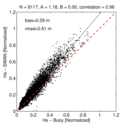
(a)

(b)

Figure 4: Normalized scatter plot and quantile-quantile plot of wave buoy $H_{\mathrm{s}}$ vs SWAN in location “SW”. Data were collected in two periods with two different buoys. The first buoy operated between 1 October and 12 November 2005. A new buoy was installed on 25 March 2006 and was in operation until 23 January 2007. The correlation found between model and wave buoy is high (0.96), but SWAN overestimates the wave height on average by 18% (bias 0.29 m).

Buoy measurements from the period 1 October to 12 November 2005 and 25 March 2006 to 23 January 2007 in location marked “SW” (see Fig. 3) have been compared with SWAN. The winter months from November 2005 to March 2006 are missing. The buoy experienced some technical difficulties during the second period and some data filtering has been carried out to remove erroneous data. The model agrees on average well with the buoy (correlation $r=0.96$), but SWAN wave heights exceed the buoy measurements (Fig. 4) by 18% (mean bias 0.29 m). SWAN also underestimates the wave period $T_{m02}$, with a bias of -0.35 s (correlation $r=0.79$). Whether the wave height bias is due to under-estimation by the buoy or over-estimation by the model is not clear, but waves coming from the exposed sector ($250-290^{\circ}$) are virtually unbiased compared with the WINCH hindcast archive in the offshore location (see Panel (c), Fig. 5 and discussion below), suggesting that the wave buoy may be underestimating the true wave height somewhat. We stress that the measurement series is short and is meant for independent evaluation of the model setup.

3 Statistical downscaling of hindcast series 1955-2006

3.1 WINCH hindcast archive

The Norwegian Meteorological Institute maintains a coarse-resolution hindcast data set covering the period 1955 and onwards. The hindcast archive is generated with a second generation wave model (WINCH, see Greenwood et al., 1985) with winds calculated in part from digitized pressure maps. The model was set up on a coarse (150 km to 75 km) grid which covered the northern North Atlantic, the Norwegian Sea, the Greenland Sea, the Barents Sea and the North Sea. The archive originally covered the period 1955-1981, but has since been updated regularly (Reistad and Iden, 1998). Although by now surpassed by more sophisticated models and forcing fields (see Reistad et al., 2007), the need for statistical stationarity in error terms still makes it worthwhile to maintain and update the archive. Here we employ the time series from the nearest grid point to perform a statistical downscaling to nearshore conditions.

3.2 Sector-wise linear downscaling

To account for the partial sheltering by islands a direction-dependent linear regression has been performed to relate the significant wave height found in the open-ocean hindcast location to the SWAN wave height found in the nearshore buoy location (see Fig. 3). The directional binning is based on the peak wave direction ($\theta_{\mathrm{p}}$) in the hindcast location. The wind direction could also be used as the binning criterion, but the wind can change rapidly and because of inertia in the wave field, wave and wind directions may in some situations differ significantly. Four directional bins have been chosen (Fig. 3), based on considerations of the differential sheltering for the various directions toward the nearshore location (coincident with buoy location). For each sector (bin) $j$, the linear regression can be written as

$$y_{j}=A_{j}x_{j}+B_{j}+e_{j},$$ (1)

where $j$ represents sectors 1, 2, 3, and 4. A time series of downscaled wave height $y_{j}$ is related to the offshore hindcast wave height, $x_{j}$, through relation (1) for each sector $j$. An aggregated time series $h$ of nearshore wave height is since constructed from these four transfer functions. The rms error $s$ of the aggregated transfer function is used to add Gaussian noise $e_{j}\in N(0,s)$ to the downscaled time series (Wilks, 1995). The transfer functions are shown in Panels (a)-(d) in Fig. 5 (summarized in Table 1). The impact of sheltering on the nearshore wave conditions and how the directional binning modifies the relation between offshore and nearshore wave height is evident. The largest reduction of wave height relative to offshore conditions appears not surprisingly in sectors $0-180^{\circ}$ and $290-360^{\circ}$. The wave height is here on average reduced to 62$\%$ and 67$\%$ of the offshore hindcast wave height, respectively. Least reduction is found in the sector $250-290^{\circ}$ (Fig. 5), where the wave height distribution nearshore is nearly identical to the offshore hindcast distribution. The total (aggregated) sector-wise transfer function is referred to as HCS. The downscaling shows good agreement with SWAN with an overall correlation coefficient $r=0.91$ (Panel (e) of Fig. 5).

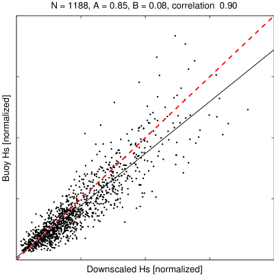
(a)

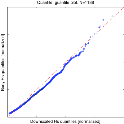
(b)

Figure 6: A comparison between the sector-wise downscaling (HCS) and buoy measurements of $H_{\mathrm{s}}$. Panel (a) shows generally good agreement with a correlation coefficient of 0.90, although the downscaling tends to over-estimate the wave height slightly. Panel (b): quantile-quantile plot.

The buoy data are used for independent evaluation of the statistical downscaling from hindcast location to the nearshore conditions at the buoy location. As seen in Panel (a) of Fig. 6, the correlation is high and comparable to the correlation against SWAN ($r=0.90$), although again a slight over-representation of the wave height is found (see also Fig. 4). This is to be expected as the downscaling relates the hindcast data to the SWAN data, hence any bias in SWAN is inherited by the downscaling. From the quantile-quantile plot in Panel (b) a slight under-representation of the very highest waves is found. Otherwise the match is good.

3.3 Return values of significant wave height

The most commonly used method for estimating return values is the “peaks-over-threshold” (POT) technique (Smith, 1990), where only maximum values exceeding a certain threshold ($u$) are kept. The assumption that the individual data points represent maxima from individual storms is usually ensured by requiring a minimum distance of 48 hours between consecutive data points (Simiu and Heckert, 1996). Let $\lambda$ represent the average number of storms per year exceeding the POT threshold $u$. Then the probability of not exceeding the $R$-year return value ($H_{R}$) in a storm is

$$F(H_{R})\equiv\mathrm{Prob}(h\leq H_{R})=1-\frac{1}{\lambda\ R}\,.$$ (2)

Thus, the probability of not exceeding for example the 100-year return value ($H_{100}$) is

$$F(H_{100})=1-\frac{1}{100\lambda}.$$

The return value $H_{R}$ should be interpreted as the value that will on average be exceeded only once in $R$ years. Wilson (1974) notes that for the Gumbel distribution, the probability of actually seeing a 100-year return value in a random 100-year period is approximately 63%. Similar values apply for the other extreme-value distributions discussed below. The threshold $u$ is manually chosen and should be high relative to typical values. Naess and Clausen (2001) suggest that optimal results are obtained if the threshold is chosen so that the number of exceedances is approximately 10 per year, while Lopatoukhin et al. (2000) suggest a threshold 2-3 times the mean value of $H_{\mathrm{s}}$. Here maxima from storms exceeding a threshold of 5 m are kept (5-7 storms per year).

Assuming that the wave heights extracted using the POT method are independent (representing maxima from different storms) and identically distributed (iid), the generalized extreme value (GEV, Jenkinson, 1955) distribution can be applied to the extremes,

$$\mbox{GEV}(h;a,b,c)=\left\{\begin{array}[]{ll}\exp\left[-(1+c\frac{h-b}{a})^{-1/c}_{+}\right]&\mbox{if $c\neq 0$}\\ \\ \exp\left[-e^{-(h-b)/a}\right]&\mbox{if $c=0$}\end{array}\right.$$ (3)

Here $h$ is the significant wave height, $a>0$ and $b$ are scale and location parameters while $c$ determines the shape of the GEV distribution. The cases $c>0$, $c=0$ and $c<0$ correspond to the Fréchet (Fisher-Tippett Type II), Gumbel (Fisher-Tippett Type I) and the reverse Weibull (Fisher-Tippett Type III) distributions, respectively. We will here estimate return values for significant wave height using the Gumbel distribution ($c=0$). In addition, the three-parameter Weibull distribution (referred to as Weibull3, not to be confused with the above-mentioned reverse Weibull or Fisher-Tippett Type III) will be used,

$$F_{w}(h)=\left\{\begin{array}[]{ll}1-\exp[-(\frac{h-b}{a})^{\gamma}]&\mbox{if $h\geq b$}\\ 0&\mbox{if $h<b$}.\end{array}\right.$$ (4)

For the Gumbel distribution, $a$ and $b$ are computed from the mean and the standard deviation of the significant wave height. For Weibull3, the location parameter $b$ is set to 4.995 m after performing an iterative best fit procedure while $a$ and $\gamma$ are determined by linear regression.

3.3.1 Ensemble estimates of return values

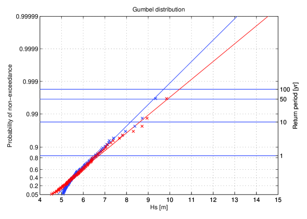
(a)

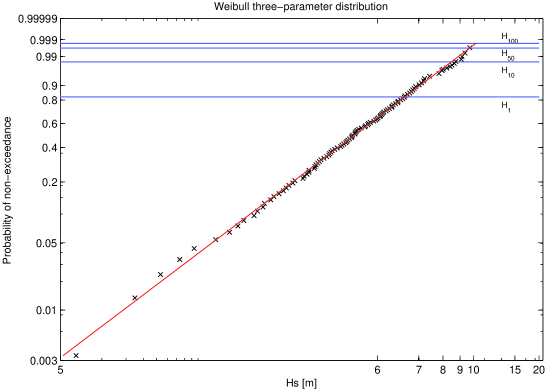
(b)

Figure 7: Peaks-over-threshold estimates of the 1, 10, 50 and 100-year return values [m] based on sectorwise statistical downscaling to nearshore conditions of 52 years of hindcast data in an open-ocean location. Panel (a): Gumbel distribution. Blue curve: no noise added to downscaling (HCS). Red curve: Ensemble estimates with Gaussian noise consistent with rms error of the downscaling is added (HCS_e). Panel (b): Three-parameter Weibull distribution, location parameter $b=4.995$m. Blue curve: no noise. Red curve: ensemble estimates with Gaussian noise added. Note that return values estimated with the Gumbel distribution are more sensitive to noise than Weibull estimates, adding 0.7 m to $H_{100}$.

Return values are sensitive to the actual shape of the cumulative distribution as well as individual extreme values. To avoid under-estimating the return values we have added Gaussian noise consistent with the rms error found in the sector-wise statistical downscaling from the hindcast location to the SWAN location. Return values denoted HCS_e in Table 2 are averages estimated from $\mathcal{O}(100)$ downscaled time series with Gaussian random noise consistent with Eq. (1) is added. This allows us to make estimates of both the mean and the spread (standard deviation) around the return values (see also Naess and Hungnes, 2002) for a similar method for estimating confidence intervals on return values). As can be seen from Table 2 and from Fig. 7 the impact of adding noise is most pronounced for estimates using the Gumbel distribution, where the 100-year return value goes up from 9.7 m to 10.4 m when noise is added to the time series. (Note that noise is added after extracting the peaks for the Gumbel method while noise is added before the selection for the Weibull3 method, since the location parameter $b$ in Eq. (4) is dependent on the threshold.) The Weibull3 method with noise gives a 100-year return value of 10.3 m and thus seems less affected by noise (10.2 m without noise, see Table 2). However, the standard deviation around this estimate is higher than for the Gumbel distribution. The 100-year return value for the significant wave height offshore is approximately 13 m (not shown). It is clear that even though the location shown in Fig. 2 is only partially sheltered by islands to the north-west and the mainland to the east, the return values are lowered significantly compared with open-ocean conditions. This reduction is not the result of damping, keep in mind that waves from the west and south-west arrive virtually unattenuated (Fig. 5), but stems instead from the fact that high waves become less likely near the coast as they can only appear from the sector $250-290^{\circ}$ whereas in the open ocean high waves can come from all directions (although the prevailing weather pattern still makes storms from the west more likely than from the east).

4 Assessment of method and concluding remarks

SWAN is seen to perform well on the spatial scales of interest, i.e., coastal semi-sheltered conditions with a spatial grid resolution of 500 m. The performance of the model was evaluated over two periods where buoy measurements were available (correlation 0.96) but with a bias of 0.29 m (18%). Running SWAN in forecast mode is thus a good alternative when detailed forecasts of wave conditions are required in regions where diagnostic, steady-state models prove inadequate, provided that a coarser, open ocean wave model is already in place. The cost of running the model is moderate, with two-day forecasts completed in less than one hour on a standard Linux workstation.

We have assessed how a nested setup with WAM and SWAN can be used to map in detail the spatial distribution of average wave climatology for partly sheltered coastal regions. To do so SWAN was integrated over a 16-month period with boundary values in the form of 2D spectra from an archived WAM model integration.

This exercise is of course much more expensive than running short (typically 48 h) daily forecasts. It is however still tractable and the results provide very detailed spatial maps of average sea state conditions. Such simulations can be carried out on a standard Linux workstation in less than one week provided wind fields and spectral boundary conditions from a coarser open-ocean wave model system have been archived. If the full nested system need be rerun, the cost goes up considerably. In our case, archived 2D spectra from pertinent locations of the nested WAM50/WAM10 forecast system were available. We emphasize that such a short (one year) model integration can only give reliable information about the average (first moment) and the second moment of the full sea state probability distribution (and even those moments can be somewhat distorted if an anomalous year is sampled). To assess the tail of the distribution, i.e., return values, a much longer integration is needed.

To estimate the extremes of the wave height distribution, the full 16-month SWAN integration was used to build a direction-dependent transfer function to the coarse hindcast location which in turn was used to statistically scale down the full 52-year time series from the hindcast archive. This allowed us a long enough series to make estimates of the extremes of the wave climatology. Using two different extreme-value distributions, the 100-year return value for the nearshore location was estimated to be around 10.3 m. This is substantially lower than what is found at the open-ocean hindcast location where the 100-year return value was found to be approximately 13 m. The cost of this additional statistical downscaling is very small, provided that a hindcast archive is in place and that a sufficiently long SWAN integration has been carried out, which in our case was done anyway to build detailed maps of average sea state conditions in the whole SWAN model domain (Fig. 3). The statistical downscaling was carried out for one particular location (where buoy data were available for reference, see Figures 2 and 3) using a sector-wise transfer function for the wave height. This procedure can be repeated for any location within the SWAN model grid at extremely little extra cost, and deliberations over which directional bins to use represent the majority of the work required to build the transfer function. It is thus a very cheap alternative to setting up a detailed diagnostic model for a region where a prognostic high-resolution model is required to estimate spatial maps of average wave climatology as described above. The correlation against wave buoy measurements is naturally somewhat lower (0.90) than those found for the SWAN simulation (0.96). More important for making realistic estimates of nearshore return values of significant wave height is the addition of Gaussian noise consistent with the rms error of the transfer function (Panel (e) of Fig. 5 and Table 1). We find that adding noise will affect the 100-year return values $H_{100}$ by as much as 0.7 m (5%).

Dynamical downscaling of hindcast data for a semi-sheltered area using nested prognostic models is found to yield good agreement with observations and to be numerically tractable. It is an efficient method to rapidly build a detailed forecast system and to determine the average wave climatology in locations where steady-state (diagnostic) wave models will not perform well because of local wave growth or where they prove impractical due to the exposure to open-ocean conditions.

The statistical downscaling for estimation of return values is numerically very efficient and yielded good agreement with observations. In conclusion we found that the combination of a fully prognostic wave forecast system which is rapidly deployable within a coarser wave forecast system and a statistical downscaling of hindcast data based on a longer model integration is well suited for building rapid environmental assessment systems for wave forecasting and hindcasting in coastal regions.

Figures and tables

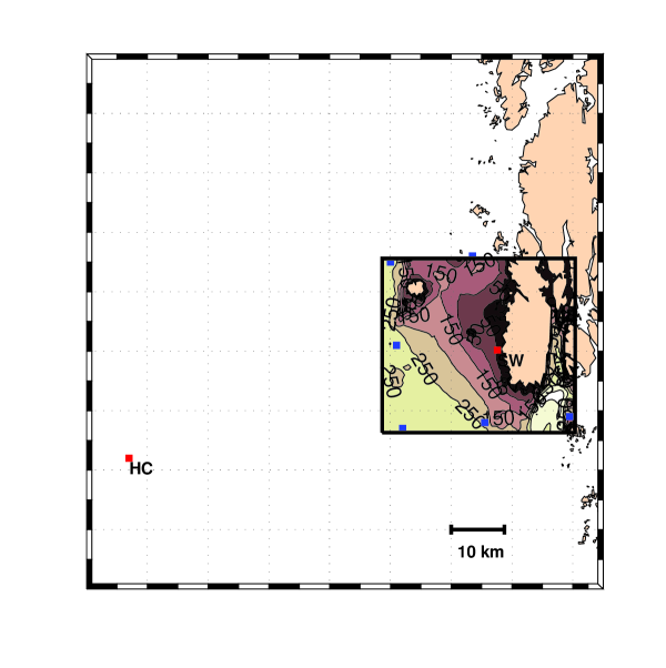
Figure 2: The SWAN model domain (500 m resolution, inner black box). The buoy location is marked as “SW”. The hindcast grid point is marked as “HC”. Blue dots indicate the location of WAM10 2D spectra used as boundary conditions for SWAN. The bathymetry of the SWAN domain is indicated with depth contours for every 50 m. The domain is only marginally affected by bottom refraction and friction.

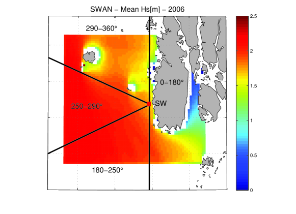
(a)

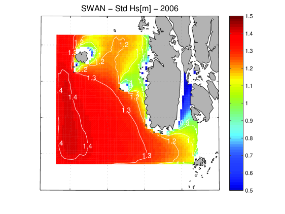
(b)

Figure 3: Panel (a): Directional binning of the nearshore location. Four sectors have been chosen to account for (1) the complete sheltering from the east, (2) the open-ocean conditions with waves propagating at a steep angle from the south and south-west, (3) the completely unsheltered conditions from the west and south-west and (4) the partial sheltering from the north and north-west by islands. The peak wave direction in the hindcast grid point is used as the selection criterion. The SWAN annual average $\overline{H_{\mathrm{s}}}$ for 2006 is seen to vary significantly throughout the model domain. The buoy location is marked as “SW”. This position is used for the statistical downscaling of the offshore hindcast data. Panel (b): Standard deviation of annual $H_{\mathrm{s}}$.

Table 1: Transfer functions between wave height offshore and nearshore for each sector; $s$ is the standard deviation of the Gaussian noise added.

Sector	Transfer function	rms error $s$ [m]
$0-180^{\circ}$:	$y=0.62x$	0.40
$180-250^{\circ}$:	$y=0.84x-0.12$	0.58
$250-290^{\circ}$:	$y=1.01x-0.20$	0.49
$290-360^{\circ}$:	$y=0.67x-0.13$	0.51

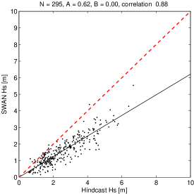
(a)	(b)
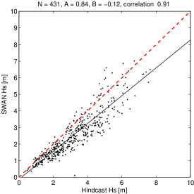
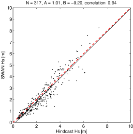
(c)	(d)
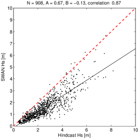
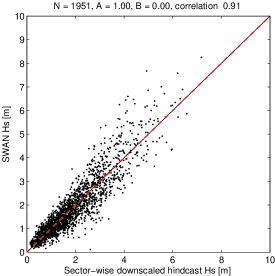
(e)	(f)

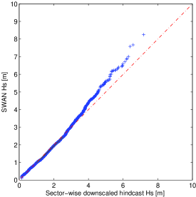
Figure 5: Sector-wise downscaling of hindcast $H_{\mathrm{s}}$ from the open-ocean location (HCS) to the SWAN nearshore location (coincident with buoy location). Panels (a)-(d) show good agreement with SWAN for the four sectors (representing $0-180^{\circ}$, $180-250^{\circ}$, $250-290^{\circ}$ and $290-360^{\circ}$, respectively), with correlation coefficients ranging from 0.88 to 0.94. Panel (e) shows the overall agreement (combined correlation 0.91) between the sectorwise downscaling of the hindcast data and the SWAN nearshore location. The rms spread is used to add Gaussian noise when estimating the return values. The quantile-quantile plot for the combined downscaling from all four sectors is shown in Panel (f), revealing a slight under-estimation of the highest waves compared with SWAN.

Table 2: Peaks-over-threshold estimates of the 1, 10, 50 and 100-year return values [m] based on sectorwise statistical downscaling to nearshore conditions of 52 years of hindcast data in an open-ocean location. Gumbel refers to the Gumbel distribution while Weibull3 refers to the three-parameter Weibull distribution with location parameter $b=4.995$m. HCS is a sectorwise downscaling with no noise added while HCS_e are ensemble averages of $\mathcal{O}(100)$ realizations where Gaussian noise consistent with the rms error in the statistical downscaling was added. The standard deviation of these estimates are included, indicating a slightly higher spread around the Weibull3 estimate.

Method	$H_{1}$	$H_{10}$	$H_{50}$	$H_{100}$	Std dev $H_{100}$ [m]
Gumbel HCS:	6.6	8.2	9.3	9.7	N/A
Gumbel HCSe:	6.8	8.6	9.9	10.4	0.12
Weibull3 HCS:	6.6	8.5	9.7	10.2	N/A
Weibull3 HCSe:	6.7	8.4	9.5	10.3	0.37

References

- Booij et al. (1999) Booij, N., Ris, R. C., Holthuijsen, L. H., 1999. A third-generation wave model for coastal regions 1. Model description and validation. J Geophys Res 104 (C4), 7649–7666.
- Gaslikova (2006) Gaslikova, L., 2006. Applications of the Dynamical and Statistical Downscaling Techniques to the Local Multi-Decade Wave Simulations. In: Proceedings of the 9th International Workshop on Wave Hindcasting and Forecasting and Coastal Hazard Symposium. p. 13.
- Gaslikova and Weisse (2006) Gaslikova, L., Weisse, R., 2006. Estimating near-shore wave statistics from regional hindcasts using downscaling techniques. Ocean Dynamics 56 (1), 26–35.
- Greenwood et al. (1985) Greenwood, J., Cardone, V., Lawson, L., 1985. Intercomparison test version of the SAIL wave model. In: group", S. (Ed.), Ocean Wave Modelling. Plenum Press, pp. 221–233.
- Hasselmann et al. (1988) Hasselmann, S., Hasselmann, K., Bauer, E., Janssen, P. A. E. M., Komen, G. J., Bertotti, L., Lionello, P., Guillaume, A., Cardone, V. C., Greenwood, J. A., Reistad, M., Zambresky, L., Ewing, J. A., 1988. The wam model—a third generation ocean wave prediction model. J Phys Oceanogr 18, 1775–1810.
- Jenkinson (1955) Jenkinson, A., 1955. The frequency distribution of the annual maximum (or minimum) values of meteorological elements. Quarterly Journal of the Royal Meteorological Society 81 (348), 158–171.
- Lopatoukhin et al. (2000) Lopatoukhin, L., Rozhkov, V., Ryabinin, V., Swail, V., Boukhanovsky, A., Degtyarev, A., 2000. Estimation of extreme wind wave heights. Tech. Rep. JCOMM Technical Report No 9, World Meteorological Organization.
- Monbaliu et al. (2000) Monbaliu, J., Padilla-Hernández, R., Hargreaves, J., Albiach, J., Luo, W., Sclavo, M., Günther, H., 2000. The spectral wave model, WAM, adapted for applications with high spatial resolution. Coastal Engineering 41 (1-3), 41–62.
- Naess and Clausen (2001) Naess, A., Clausen, P., 2001. Combination of the peaks-over-treshold and bootstrapping methods for extreme value prediction. Structural Safety 23, 315–330.
- Naess and Hungnes (2002) Naess, A., Hungnes, B., 2002. Estimating Confidence Intervals of Long Return Period Design Values by Bootstrapping. Journal of Offshore Mechanics and Arctic Engineering 124, 5, doi:10.1115/1.1446078.
- O’Reilly and Guza (1993) O’Reilly, W., Guza, R., 1993. A comparison of two spectral wave models in the Southern California Bight. Coastal Engineering 19 (3), 263–282.
- Reistad et al. (2007) Reistad, M., Breivik, Ø., Haakenstad, H., 2007. A High-Resolution Hindcast Study for the North Sea, the Norwegian Sea and the Barents Sea. In: Proceedings of the 10th International Workshop on Wave Hindcasting and Forecasting and Coastal Hazard Symposium. p. 13.
- Reistad and Iden (1998) Reistad, M., Iden, K., 1998. Updating, correction and evaluation of a hindcast data base of air pressure, wind and waves for the North Sea, the Norwegian Sea and the Barents Sea. Tech. Rep. 9, The Norwegian Meteorological Institute, Oslo.
- Ris et al. (1999) Ris, R. C., Holthuijsen, L. H., Booij, N., 1999. A third-generation wave model for coastal regions 2. Verification. J Geophys Res 104 (C4), 7667–7681.
- Simiu and Heckert (1996) Simiu, E., Heckert, N., 1996. Extreme wind distribution tails: A peaks over threshold approach. Journal of structural engineering 122 (5), 539–547.
- Smith et al. (2001) Smith, J., Sherlock, A., Resio, D., 2001. STWAVE: Steady-state Spectral Wave Model User’s Manual for STWAVE, Version 3.0. Tech. rep., US Army Corps of Engineers, Engineer Research and Development Center.
- Smith (1990) Smith, R., 1990. Extreme value theory. In: Ledermann, E., Lloyd, E., Vajda, S., Alexander, C. (Eds.), Handbook of Applicable Mathematics. Wiley, pp. 437–471.
- Stoelinga and Warner (1999) Stoelinga, M. T., Warner, T. T., 1999. Nonhydrostatic, mesobeta-scale model simulations of cloud ceiling and visibility for an East Coast winter precipitation event. J Appl Meteor 38 (4), 385–404.
- Tolman (1991) Tolman, H. L., 1991. A Third-Generation Model for Wind Waves on Slowly Varying, Unsteady, and Inhomogeneous Depths and Currents. J Phys Oceanogr 21 (6), 782–797.
- Unden et al. (2002) Unden, P., Rontu, L., Jarvinen, H., Lynch, P., Calvo, J., Cats, G., Cuxart, J., Eerola, K., Fortelius, C., Garcia-Moya, J. A., Jones, C., Lenderink, G., Mc-Donald, A., McGrath, R., Navascues, B., Nielsen, N. W., Odegaard, V., Rodriguez, E., Rummukainen, M., Room, R., Sattler, K., Savijarvi, H., Sass, B. H., Schreur, B. W., The, H., Tijm, S., 2002. Hirlam-5 scientific documentation. Tech. Rep. GKSS 97/E/46, SMHI, SMHI, SE-601 76 Norrkoping, Sweden.
- Wilks (1995) Wilks, D. S., 1995. Statistical Methods in the Atmospheric Sciences. Academic Press, London.
- Wilson (1974) Wilson, E. M., 1974. Engineering hydrology. Macmillan, London.