Relativistic Burgers equations on curved spacetimes. Derivation and finite volume approximation

Philippe G. LeFloch Laboratoire Jacques–Louis Lions & Centre National de la Recherche Scientifique, Université Pierre et Marie Curie (Paris 6), 4 Place Jussieu, 75252 Paris, France. (contact@philippelefloch.org, makhlof@ann.jussieu.fr)    Hasan Makhlof    Baver Okutmustur
2000 AMS Subject Class. 35L65
Department of Mathematics, Middle East Technical University, 06800 Ankara, Turkey. (baver@metu.edu.tr)
   76N10    83A05.
Keywords. Nonlinear hyperbolic
   balance law    curved spacetime    relativistic Burgers equation    well balanced
Abstract

Within the class of nonlinear hyperbolic balance laws posed on a curved spacetime (endowed with a volume form), we identify a hyperbolic balance law that enjoys the same Lorentz invariance property as the one satisfied by the Euler equations of relativistic compressible fluids. This model is unique up to normalization and converges to the standard inviscid Burgers equation in the limit of infinite light speed. Furthermore, from the Euler system of relativistic compressible flows on a curved background, we derive both the standard inviscid Burgers equation and our relativistic generalizations. The proposed models are referred to as relativistic Burgers equations on curved spacetimes and provide us with simple models on which numerical methods can be developed and analyzed. Next, we introduce a finite volume scheme for the approximation of discontinuous solutions to these relativistic Burgers equations. Our scheme is formulated geometrically and is consistent with the natural divergence form of the balance laws under consideration. It applies to weak solutions containing shock waves and, most importantly, is well balanced in the sense that it preserves steady solutions. Numerical experiments are presented which demonstrate the convergence of the proposed finite volume scheme and its relevance for computing entropy solutions on a curved background.

1 Introduction

In computational fluid dynamics, the (inviscid) Burgers equation

tu+x(u2/2)=0,u=u(t,x),t>0,x,formulae-sequencesubscript𝑡𝑢subscript𝑥superscript𝑢220formulae-sequence𝑢𝑢𝑡𝑥formulae-sequence𝑡0𝑥\partial_{t}u+\partial_{x}\big{(}u^{2}/2\big{)}=0,\qquad u=u(t,x),\quad t>0,\,x\in\mathbb{R},

is an important toy model, which can be formally derived from the Euler equations of compressible fluids

tρ+x(ρu)=0,t(ρu)+x(ρu2+p(ρ))=0,formulae-sequencesubscript𝑡𝜌subscript𝑥𝜌𝑢0subscript𝑡𝜌𝑢subscript𝑥𝜌superscript𝑢2𝑝𝜌0\partial_{t}\rho+\partial_{x}(\rho u)=0,\qquad\quad\partial_{t}(\rho u)+\partial_{x}(\rho u^{2}+p(\rho))=0,

(ρ,u𝜌𝑢\rho,u denoting the density and velocity of the fluid and p=p(ρ)𝑝𝑝𝜌p=p(\rho) its pressure). The Burgers equation is also the simplest example of nonlinear hyperbolic conservation law and has played an essential role in the development of robust and accurate, shock-capturing schemes for the approximation of entropy solutions to nonlinear hyperbolic systems.

In the present paper, we derive several relativistic generalizations of Burgers equation which, in addition, we formulate on a curved background, and we study the discretization of these equations via a well balanced, finite volume strategy based on time–independent solutions to these relativistic Burgers equations. More precisely, we consider the following class of nonlinear hyperbolic balance laws

divω(T(v))=S(v),subscriptdiv𝜔𝑇𝑣𝑆𝑣\mbox{div}_{\omega}(T(v))=S(v), (1)

posed on an (n+1)𝑛1(n+1)-dimensional curved spacetime (with boundary), denoted by (M,ω)𝑀𝜔(M,\omega) and endowed with a volume form ω𝜔\omega. The unknown function is a scalar field v:M:𝑣𝑀v:M\to\mathbb{R} and divωsubscriptdiv𝜔\mbox{div}_{\omega} denotes the divergence operator associated with the volume form. The flux vector field T=T(v)𝑇𝑇𝑣T=T(v) is a field of tangent vectors prescribed on M𝑀M and depending smoothly upon v𝑣v, while the right–hand side S=S(v)𝑆𝑆𝑣S=S(v) is a scalar field prescribed on M𝑀M which also smoothly depends upon v𝑣v.

Hyperbolic conservation laws on curved spacetimes have been analyzed in recent years by LeFloch and collaborators; cf. the review [5], as well as [1, 2, 7]. In order to formulate the initial value problem for (1), we assume that the spacetime is foliated by hypersurfaces, that is,

M=t0Ht,𝑀subscript𝑡0subscript𝐻𝑡M=\bigcup_{t\geq 0}H_{t}, (2)

in which each slice Htsubscript𝐻𝑡H_{t} is an n𝑛n-dimensional manifold, canonically endowed with a normal 111-form field Ntsubscript𝑁𝑡N_{t} and with the same topology as the one of the initial slice H0subscript𝐻0H_{0}. The global hyperbolicity of the spacetime and the equation (1), by definition, requires that each slice Htsubscript𝐻𝑡H_{t} be spacelike, in the sense that the function

vT0(v):=Nt,T(v) is strictly increasing.formulae-sequencemaps-to𝑣superscript𝑇0𝑣assignsubscript𝑁𝑡𝑇𝑣 is strictly increasing.v\mapsto T^{0}(v):=\langle N_{t},T(v)\rangle\quad\mbox{ is strictly increasing.} (3)

The class of nonlinear hyperbolic equations (1)–(3) provides us with a scalar model on which one can develop and analyze numerical methods of approximations which are then applicable to the Euler equations of relativistic compressible fluid flows on a curved spacetime. We refer the reader to the follow–up work by LeFloch and Makhlof [6] which addresses this generalization. For the well posedness theory of the initial value problem associated with (1), we refer the reader to [1] and the references cited therein.

In this paper, we introduce a geometric formulation of the finite volume method, which is classically formulated without taking the underlying geometry into account, and we formulate a well balanced version of this method, which is inspired from the work of Russo and collaborators [10, 11, 12, 13] and is built upon the Nessyahu–Tadmor scheme [9]. For a review on well balanced techniques, we refer the reader to Bouchut [3], Greenberg and Leroux [4], and LeVeque [8].

An outline of the present paper is as follows. In Section 2, we derive our relativistic version of Burgers equation when all geometric effects are neglected. In Section 3, we explain how to take the geometry into account and we also connect our model to the Euler equations. Next, in Section 4, we present the finite volume strategy, and finally, in Section 5, several numerical experiments. Section 6 contains concluding remarks on this paper.

2 A Lorentz–invariant conservation law

2.1 Derivation of the new model

In this section, we search for flux vector fields T=T(v)𝑇𝑇𝑣T=T(v) for which solutions to the equation (1) satisfy the same Lorentz invariant property as the solutions to the Euler equations of relativistic fluids. For the sake of simplicity in the presentation (and without loss of generality for the purpose of this section), we assume that n=1𝑛1n=1, S(v)0𝑆𝑣0S(v)\equiv 0, and that the manifold M=[0,+)×𝑀0M=[0,+\infty)\times\mathbb{R} is covered by a (single) coordinate chart (x0,x1)superscript𝑥0superscript𝑥1(x^{0},x^{1}) in which the volume form reads ω=dx0dx1𝜔𝑑superscript𝑥0𝑑superscript𝑥1\omega=dx^{0}dx^{1}. Hence, (1) takes the simplest form of a hyperbolic conservation law, i.e.

0T0(v)+1T1(v)=0,subscript0superscript𝑇0𝑣subscript1superscript𝑇1𝑣0\partial_{0}T^{0}(v)+\partial_{1}T^{1}(v)=0,

with 0=/x0subscript0superscript𝑥0\partial_{0}=\partial/\partial x^{0} and 1=/x1subscript1superscript𝑥1\partial_{1}=\partial/\partial x^{1}, while x0[0,+)superscript𝑥00x^{0}\in[0,+\infty) and x1superscript𝑥1x^{1}\in\mathbb{R}. In addition, in the present section, we also assume that the functions T0=T0(v)superscript𝑇0superscript𝑇0𝑣T^{0}=T^{0}(v) and T1=T1(v)superscript𝑇1superscript𝑇1𝑣T^{1}=T^{1}(v) are independent of (x0,x1)superscript𝑥0superscript𝑥1(x^{0},x^{1}). A formulation taking geometric effects into account will be introduced and investigated in Section 3, below.

The Lorentz transformation (x0,x1)(x¯0,x¯1)maps-tosuperscript𝑥0superscript𝑥1superscript¯𝑥0superscript¯𝑥1(x^{0},x^{1})\mapsto(\overline{x}^{0},\overline{x}^{1}) reads

x¯0:=γϵ(V)(x0ϵ2Vx1),x¯1:=γϵ(V)(Vx0+x1),formulae-sequenceassignsuperscript¯𝑥0subscript𝛾italic-ϵ𝑉superscript𝑥0superscriptitalic-ϵ2𝑉superscript𝑥1assignsuperscript¯𝑥1subscript𝛾italic-ϵ𝑉𝑉superscript𝑥0superscript𝑥1\overline{x}^{0}:=\gamma_{\epsilon}(V)\,\big{(}x^{0}-\epsilon^{2}Vx^{1}\big{)},\qquad\quad\overline{x}^{1}:=\gamma_{\epsilon}(V)\,\big{(}-V\,x^{0}+x^{1}\big{)}, (4)

where ϵ(1,1)italic-ϵ11\epsilon\in(-1,1) denotes the inverse of the (normalized) speed of light, and γϵ(V)=(1ϵ2V2)1/2subscript𝛾italic-ϵ𝑉superscript1superscriptitalic-ϵ2superscript𝑉212\gamma_{\epsilon}(V)=\big{(}1-\epsilon^{2}\,V^{2}\big{)}^{-1/2} the so-called Lorentz factor associated with a given speed V(1/ϵ,1/ϵ)𝑉1italic-ϵ1italic-ϵV\in(-1/\epsilon,1/\epsilon). These equations can be inverted to give

x0=γϵ(V)(x¯0+ϵ2Vx¯1),x1=γϵ(V)(Vx¯0+x¯1).formulae-sequencesuperscript𝑥0subscript𝛾italic-ϵ𝑉superscript¯𝑥0superscriptitalic-ϵ2𝑉superscript¯𝑥1superscript𝑥1subscript𝛾italic-ϵ𝑉𝑉superscript¯𝑥0superscript¯𝑥1x^{0}=\gamma_{\epsilon}(V)\,\big{(}\overline{x}^{0}+\epsilon^{2}V\overline{x}^{1}\big{)},\qquad\quad x^{1}=\gamma_{\epsilon}(V)\,\big{(}V\,\overline{x}^{0}+\overline{x}^{1}\big{)}.

Instead of V𝑉V, it is often convenient to use the normalized speed U𝑈U\in\mathbb{R} defined by

eϵU:=γϵ(V)(1+ϵV)=(1+ϵV1ϵV)1/2,assignsuperscript𝑒italic-ϵ𝑈subscript𝛾italic-ϵ𝑉1italic-ϵ𝑉superscript1italic-ϵ𝑉1italic-ϵ𝑉12e^{\epsilon U}:=\gamma_{\epsilon}(V)\,(1+\epsilon\,V)=\Bigg{(}{1+\epsilon V\over 1-\epsilon V}\Bigg{)}^{1/2},

so that the Lorentz transformation takes the compact form x¯0±ϵx¯1=eϵU(x0±ϵx1)plus-or-minussuperscript¯𝑥0italic-ϵsuperscript¯𝑥1superscript𝑒minus-or-plusitalic-ϵ𝑈plus-or-minussuperscript𝑥0italic-ϵsuperscript𝑥1{\overline{x}^{0}\pm\epsilon\,\overline{x}^{1}}={e^{\mp\epsilon U}\,(x^{0}\pm\epsilon\,x^{1})} or, equivalently,

x¯0=cosh(ϵU)x0ϵsinh(ϵU)x1,x¯1=1ϵsinh(ϵU)x0+cosh(ϵU)x1,formulae-sequencesuperscript¯𝑥0italic-ϵ𝑈superscript𝑥0italic-ϵitalic-ϵ𝑈superscript𝑥1superscript¯𝑥11italic-ϵitalic-ϵ𝑈superscript𝑥0italic-ϵ𝑈superscript𝑥1\overline{x}^{0}=\cosh(\epsilon U)\,x^{0}-\epsilon\,\sinh(\epsilon U)\,x^{1},\qquad\quad\overline{x}^{1}=-{\frac{1}{\epsilon}}\sinh(\epsilon U)\,x^{0}+\cosh(\epsilon U)\,x^{1}, (5)

with cosh(ϵU)=γϵ(V)italic-ϵ𝑈subscript𝛾italic-ϵ𝑉\cosh(\epsilon U)=\gamma_{\epsilon}(V) and sinh(ϵU)=ϵVγϵ(V)italic-ϵ𝑈italic-ϵ𝑉subscript𝛾italic-ϵ𝑉\sinh(\epsilon U)=\epsilon V\,\gamma_{\epsilon}(V). Recall also that the set of Lorentz transformations (together with the spatial rotations if n2𝑛2n\geq 2) forms the so-called Lorentz isometry group, characterized by the condition that the length element of the Minkowski metric is preserved, that is, ϵ2(x¯0)2+(x¯1)2=ϵ2(x0)2+(x1)2.superscriptitalic-ϵ2superscriptsuperscript¯𝑥02superscriptsuperscript¯𝑥12superscriptitalic-ϵ2superscriptsuperscript𝑥02superscriptsuperscript𝑥12-\epsilon^{-2}\,(\overline{x}^{0})^{2}+(\overline{x}^{1})^{2}=-\epsilon^{-2}\,(x^{0})^{2}+(x^{1})^{2}. The relativistic Euler equations of compressible fluids are invariant under the Lorentz transformation (4). More precisely, given a speed V𝑉V, the fluid velocity component v𝑣v in the coordinate system (x0,x1)superscript𝑥0superscript𝑥1(x^{0},x^{1}) is related to the component v¯¯𝑣\overline{v} in the coordinates (x¯0,x¯1)superscript¯𝑥0superscript¯𝑥1(\overline{x}^{0},\overline{x}^{1}) by the relation

v¯=vV1ϵ2Vv.¯𝑣𝑣𝑉1superscriptitalic-ϵ2𝑉𝑣\overline{v}={v-V\over 1-\epsilon^{2}V\,v}. (6)

Clearly, in the nonrelativistic limit ϵ0italic-ϵ0\epsilon\to 0, one recovers the Galilean transformation

x¯0=x0,x¯1=Vx0+x1,v¯=vV when ϵ=0,formulae-sequencesuperscript¯𝑥0superscript𝑥0formulae-sequencesuperscript¯𝑥1𝑉superscript𝑥0superscript𝑥1formulae-sequence¯𝑣𝑣𝑉 when italic-ϵ0\overline{x}^{0}=x^{0},\quad\overline{x}^{1}=-V\,x^{0}+x^{1},\qquad\overline{v}=v-V\quad\mbox{ when }\epsilon=0, (7)

in which the speed V𝑉V belongs to \mathbb{R}.

Theorem 1 (Relativistic version of Burgers equation).

The conservation law

0T0(v)+1T1(v)=0subscript0superscript𝑇0𝑣subscript1superscript𝑇1𝑣0\partial_{0}T^{0}(v)+\partial_{1}T^{1}(v)=0 (8)

is invariant under the Lorentz transformations (5)–(6) if and only if, after suitable normalization (discussed below), one has

T0(v)=v1ϵ2v2,T1(v)=1ϵ2(1+11ϵ2v2),formulae-sequencesuperscript𝑇0𝑣𝑣1superscriptitalic-ϵ2superscript𝑣2superscript𝑇1𝑣1superscriptitalic-ϵ2111superscriptitalic-ϵ2superscript𝑣2T^{0}(v)=\frac{v}{\sqrt{1-\epsilon^{2}v^{2}}},\qquad T^{1}(v)=\frac{1}{\epsilon^{2}}\Bigg{(}-1+\frac{1}{\sqrt{1-\epsilon^{2}v^{2}}}\Bigg{)}, (9)

where the unknown scalar field v𝑣v takes its value in the interval (1/ϵ,1/ϵ)1italic-ϵ1italic-ϵ(-1/\epsilon,1/\epsilon).

We refer to (8)–(9) as the relativistic Burgers equations (on Minkowski spacetime).

Proof. We first change coordinates and construct certain auxilliary functions, denoted below by H±(v)subscript𝐻plus-or-minus𝑣H_{\pm}(v). Precisely, in the coordinates (x0,x1)superscript𝑥0superscript𝑥1(x^{0},x^{1}), we can differentiate the Lorentz expressions (4) and obtain

x¯0x0superscript¯𝑥0superscript𝑥0\displaystyle\frac{\partial\overline{x}^{0}}{\partial x^{0}} =11ϵ2V2=γϵ(V),absent11superscriptitalic-ϵ2superscript𝑉2subscript𝛾italic-ϵ𝑉\displaystyle=\frac{1}{\sqrt{1-\epsilon^{2}\,V^{2}}}=\gamma_{\epsilon}(V),\qquad\qquad\, x¯0x1=ϵ2Vγϵ(V),superscript¯𝑥0superscript𝑥1superscriptitalic-ϵ2𝑉subscript𝛾italic-ϵ𝑉\displaystyle\frac{\partial\overline{x}^{0}}{\partial x^{1}}=-\epsilon^{2}\,V\gamma_{\epsilon}(V),
x¯1x0superscript¯𝑥1superscript𝑥0\displaystyle\frac{\partial\overline{x}^{1}}{\partial x^{0}} =Vγϵ(V),absent𝑉subscript𝛾italic-ϵ𝑉\displaystyle\hskip-54.06006pt=-V\,\gamma_{\epsilon}(V),\qquad x¯1x1=γϵ(V)superscript¯𝑥1superscript𝑥1subscript𝛾italic-ϵ𝑉\displaystyle\frac{\partial\overline{x}^{1}}{\partial x^{1}}=\gamma_{\epsilon}(V)

and, by the chain rule,

0T0subscript0superscript𝑇0\displaystyle\partial_{0}T^{0} =\displaystyle= T0x¯0x¯0x0+T0x¯1x¯1x0=T0x¯0γϵ(V)T0x¯1γϵ(V)V,superscript𝑇0superscript¯𝑥0superscript¯𝑥0superscript𝑥0superscript𝑇0superscript¯𝑥1superscript¯𝑥1superscript𝑥0superscript𝑇0superscript¯𝑥0subscript𝛾italic-ϵ𝑉superscript𝑇0superscript¯𝑥1subscript𝛾italic-ϵ𝑉𝑉\displaystyle\frac{\partial T^{0}}{\partial\overline{x}^{0}}\frac{\partial\overline{x}^{0}}{\partial x^{0}}+\frac{\partial T^{0}}{\partial\overline{x}^{1}}\frac{\partial\overline{x}^{1}}{\partial x^{0}}=\frac{\partial T^{0}}{\partial\overline{x}^{0}}\gamma_{\epsilon}(V)-\frac{\partial T^{0}}{\partial\overline{x}^{1}}\gamma_{\epsilon}(V)\,V,
1T1subscript1superscript𝑇1\displaystyle\partial_{1}T^{1} =\displaystyle= T1x¯0x¯0x1+T1x¯1x¯1x1=ϵ2T1x¯0γϵ(V)V+T1x¯1γϵ(V).superscript𝑇1superscript¯𝑥0superscript¯𝑥0superscript𝑥1superscript𝑇1superscript¯𝑥1superscript¯𝑥1superscript𝑥1superscriptitalic-ϵ2superscript𝑇1superscript¯𝑥0subscript𝛾italic-ϵ𝑉𝑉superscript𝑇1superscript¯𝑥1subscript𝛾italic-ϵ𝑉\displaystyle\frac{\partial T^{1}}{\partial\overline{x}^{0}}\frac{\partial\overline{x}^{0}}{\partial x^{1}}+\frac{\partial T^{1}}{\partial\overline{x}^{1}}\frac{\partial\overline{x}^{1}}{\partial x^{1}}=-\epsilon^{2}\,\frac{\partial T^{1}}{\partial\overline{x}^{0}}\gamma_{\epsilon}(V)\,V+\frac{\partial T^{1}}{\partial\overline{x}^{1}}\gamma_{\epsilon}(V).

By substituting these formulas in (8), the conservation law reads

0=0T0+1T1=0(γϵ(V)T0ϵ2γϵ(V)VT1)+1(Vγϵ(V)T0+γϵ(V)T1),0subscript0superscript𝑇0subscript1superscript𝑇1subscript0subscript𝛾italic-ϵ𝑉superscript𝑇0superscriptitalic-ϵ2subscript𝛾italic-ϵ𝑉𝑉superscript𝑇1subscript1𝑉subscript𝛾italic-ϵ𝑉superscript𝑇0subscript𝛾italic-ϵ𝑉superscript𝑇1\displaystyle 0=\partial_{0}T^{0}+\partial_{1}T^{1}=\partial_{0}(\gamma_{\epsilon}(V)\,T^{0}-\epsilon^{2}\,\gamma_{\epsilon}(V)\,V\,T^{1})+\partial_{1}(-V\,\gamma_{\epsilon}(V)\,T^{0}+\gamma_{\epsilon}(V)\,T^{1}),

which has the same structure as (8) in the coordinates (x¯0,x¯1)superscript¯𝑥0superscript¯𝑥1(\overline{x}^{0},\overline{x}^{1}) provided

γϵ(V)(T0(v)ϵ2VT1(v))subscript𝛾italic-ϵ𝑉superscript𝑇0𝑣superscriptitalic-ϵ2𝑉superscript𝑇1𝑣\displaystyle\gamma_{\epsilon}(V)\,\big{(}T^{0}(v)-\epsilon^{2}V\,T^{1}(v)\big{)} =T0(vV1ϵ2vV)+C1,absentsuperscript𝑇0𝑣𝑉1superscriptitalic-ϵ2𝑣𝑉subscript𝐶1\displaystyle=T^{0}\Bigg{(}\frac{v-V}{1-\epsilon^{2}v\,V}\Bigg{)}+C_{1}, (10)
γϵ(V)(VT0(v)+T1(v))subscript𝛾italic-ϵ𝑉𝑉superscript𝑇0𝑣superscript𝑇1𝑣\displaystyle\gamma_{\epsilon}(V)\,\big{(}-VT^{0}(v)+T^{1}(v)\big{)} =T1(vV1ϵ2vV)+C2,absentsuperscript𝑇1𝑣𝑉1superscriptitalic-ϵ2𝑣𝑉subscript𝐶2\displaystyle=T^{1}\Bigg{(}\frac{v-V}{1-\epsilon^{2}v\,V}\Bigg{)}+C_{2}, (11)

for some constants C1,C2subscript𝐶1subscript𝐶2C_{1},C_{2}. This leads us to the desired invariance property and it remains to determine the general expressions of T0,T1superscript𝑇0superscript𝑇1T^{0},T^{1}.

We can always normalize the flux terms so that T0(0)=T1(0)=0,superscript𝑇00superscript𝑇100T^{0}(0)=T^{1}(0)=0, and then observe that the constants C1=T0(V)subscript𝐶1superscript𝑇0𝑉C_{1}=-T^{0}(-V) and C2=T1(V)subscript𝐶2superscript𝑇1𝑉C_{2}=-T^{1}(-V) are determined as functions of V𝑉V. Next, multiplying the second equation in (10) by ±ϵplus-or-minusitalic-ϵ\pm\epsilon and summing up with the first one, we find

γϵ(V)(1ϵV)(T0±ϵT1)(v)=(T0±ϵT1)(vV1ϵ2vV)(T0±ϵT1)(V).subscript𝛾italic-ϵ𝑉minus-or-plus1italic-ϵ𝑉plus-or-minussuperscript𝑇0italic-ϵsuperscript𝑇1𝑣plus-or-minussuperscript𝑇0italic-ϵsuperscript𝑇1𝑣𝑉1superscriptitalic-ϵ2𝑣𝑉plus-or-minussuperscript𝑇0italic-ϵsuperscript𝑇1𝑉\gamma_{\epsilon}(V)\,(1\mp\epsilon V)(T^{0}\pm\epsilon\,T^{1})(v)=\big{(}T^{0}\pm\epsilon\,T^{1}\big{)}\,\Bigg{(}\frac{v-V}{1-\epsilon^{2}\,vV}\Bigg{)}-(T^{0}\pm\epsilon\,T^{1})(-V).

By setting (T0±ϵT1)=:H±(T^{0}\pm\epsilon\,T^{1})=:H_{\pm}, these two equations read

H±(v)=1±ϵV1ϵV(H±(vV1ϵ2vV)H±(V)).subscript𝐻plus-or-minus𝑣plus-or-minus1italic-ϵ𝑉minus-or-plus1italic-ϵ𝑉subscript𝐻plus-or-minus𝑣𝑉1superscriptitalic-ϵ2𝑣𝑉subscript𝐻plus-or-minus𝑉H_{\pm}(v)=\sqrt{\frac{1\pm\epsilon V}{1\mp\epsilon V}}\,\Bigg{(}H_{\pm}\Big{(}\frac{v-V}{1-\epsilon^{2}\,vV}\Big{)}-H_{\pm}(-V)\Bigg{)}. (12)

Next, we define the new variables

u:=12ϵln(1+ϵv1ϵv),ϕϵ(u):=v,ϕϵ(U):=V,formulae-sequenceassign𝑢12italic-ϵ1italic-ϵ𝑣1italic-ϵ𝑣formulae-sequenceassignsubscriptitalic-ϕitalic-ϵ𝑢𝑣assignsubscriptitalic-ϕitalic-ϵ𝑈𝑉u:=\frac{1}{2\epsilon}\ln\Big{(}{\frac{1+\epsilon v}{1-\epsilon v}}\Big{)},\qquad\phi_{\epsilon}(u):=v,\quad\phi_{\epsilon}(U):=V,

so that

v=1ϵe2ϵu1e2ϵu+1=ϕϵ(u),v¯=1ϵe2ϵ(uU)1e2ϵ(uU)+1=ϕϵ(uU),1±ϵV1ϵV=e±ϵU.formulae-sequence𝑣1italic-ϵsuperscript𝑒2italic-ϵ𝑢1superscript𝑒2italic-ϵ𝑢1subscriptitalic-ϕitalic-ϵ𝑢¯𝑣1italic-ϵsuperscript𝑒2italic-ϵ𝑢𝑈1superscript𝑒2italic-ϵ𝑢𝑈1subscriptitalic-ϕitalic-ϵ𝑢𝑈plus-or-minus1italic-ϵ𝑉minus-or-plus1italic-ϵ𝑉superscript𝑒plus-or-minusitalic-ϵ𝑈v=\frac{1}{\epsilon}\frac{e^{2\epsilon u}-1}{e^{2\epsilon u}+1}=\phi_{\epsilon}(u),\qquad\overline{v}=\frac{1}{\epsilon}\frac{e^{2\epsilon(u-U)}-1}{e^{2\epsilon(u-U)}+1}=\phi_{\epsilon}(u-U),\qquad\sqrt{\frac{1\pm\epsilon V}{1\mp\epsilon V}}=e^{\pm\,\epsilon U}.

By inserting these expressions in (12), it follows that

H±(ϕϵ(u))H±(ϕϵ(0))=e±ϵU(H±(ϕϵ(uU))H±(ϕϵ(U))).subscript𝐻plus-or-minussubscriptitalic-ϕitalic-ϵ𝑢subscript𝐻plus-or-minussubscriptitalic-ϕitalic-ϵ0superscript𝑒plus-or-minusitalic-ϵ𝑈subscript𝐻plus-or-minussubscriptitalic-ϕitalic-ϵ𝑢𝑈subscript𝐻plus-or-minussubscriptitalic-ϕitalic-ϵ𝑈H_{\pm}\big{(}\phi_{\epsilon}(u)\big{)}-H_{\pm}\big{(}\phi_{\epsilon}(0)\big{)}=e^{\pm\,\epsilon U}\Big{(}H_{\pm}\big{(}\phi_{\epsilon}(u-U)\big{)}-H_{\pm}\big{(}\phi_{\epsilon}(-U)\big{)}\Big{)}. (13)

Abusing notation, we write H,ϕ,eϵU𝐻italic-ϕsuperscript𝑒italic-ϵ𝑈H,\phi,e^{\epsilon U} instead of H±,ϕϵ,e±ϵUsubscript𝐻plus-or-minussubscriptitalic-ϕitalic-ϵsuperscript𝑒plus-or-minusitalic-ϵ𝑈H_{\pm},\phi_{\epsilon},e^{\pm\epsilon U}, respectively. We differentiate (13) with respect to u𝑢u and obtain H(ϕ(u))ϕ(u)=eϵUH(ϕ(uU))ϕ(uU)superscript𝐻italic-ϕ𝑢superscriptitalic-ϕ𝑢superscript𝑒italic-ϵ𝑈superscript𝐻italic-ϕ𝑢𝑈superscriptitalic-ϕ𝑢𝑈H^{\prime}\big{(}\phi(u)\big{)}\phi^{\prime}(u)=e^{\epsilon U}H^{\prime}\big{(}\phi(u-U)\big{)}\phi^{\prime}(u-U) and, next, with respect to U𝑈U

H′′(ϕ(uU))(ϕ(uU))2=ϵH(ϕ(uU))ϕ(uU)ϕ′′(uU)H(ϕ(uU)).superscript𝐻′′italic-ϕ𝑢𝑈superscriptsuperscriptitalic-ϕ𝑢𝑈2italic-ϵsuperscript𝐻italic-ϕ𝑢𝑈superscriptitalic-ϕ𝑢𝑈superscriptitalic-ϕ′′𝑢𝑈superscript𝐻italic-ϕ𝑢𝑈H^{\prime\prime}\big{(}\phi(u-U)\big{)}\big{(}\phi^{\prime}(u-U)\big{)}^{2}=\epsilon H^{\prime}\big{(}\phi(u-U)\big{)}\phi^{\prime}(u-U)-\phi^{\prime\prime}(u-U)H^{\prime}\big{(}\phi(u-U)\big{)}.

By letting U=0𝑈0U=0, it follows that H′′(ϕ(u))(ϕ(u))2=ϵH(ϕ(u))ϕ(u)ϕ′′(u)H(ϕ(u))superscript𝐻′′italic-ϕ𝑢superscriptsuperscriptitalic-ϕ𝑢2italic-ϵsuperscript𝐻italic-ϕ𝑢superscriptitalic-ϕ𝑢superscriptitalic-ϕ′′𝑢superscript𝐻italic-ϕ𝑢H^{\prime\prime}\big{(}\phi(u)\big{)}\big{(}\phi^{\prime}(u)\big{)}^{2}=\epsilon H^{\prime}\big{(}\phi(u)\big{)}\phi^{\prime}(u)-\phi^{\prime\prime}(u)H^{\prime}\big{(}\phi(u)\big{)}. The substitution K(u):=H(ϕ(u))assign𝐾𝑢𝐻italic-ϕ𝑢K(u):=H(\phi(u)) allows us to rewrite the latter equation as K′′(u)=ϵK(u)superscript𝐾′′𝑢italic-ϵsuperscript𝐾𝑢K^{\prime\prime}(u)=\epsilon\,K^{\prime}(u), which has the following general solution (in which c,c~𝑐~𝑐c,\widetilde{c} are constants):

K(u)=ceϵuϵ+c~.𝐾𝑢𝑐superscript𝑒italic-ϵ𝑢italic-ϵ~𝑐K(u)=c\frac{e^{\epsilon u}}{\epsilon}+\widetilde{c}.

Alternatively, this latter relation can be derived by dividing (13) by u0𝑢0u\neq 0 and letting u0𝑢0u\to 0.

Returning to H±subscript𝐻plus-or-minusH_{\pm}, we deduce that there exist constants so that H±(ϕ(u))=±ϵ1(e±ϵu1)subscript𝐻plus-or-minusitalic-ϕ𝑢plus-or-minussuperscriptitalic-ϵ1superscript𝑒plus-or-minusitalic-ϵ𝑢1H_{\pm}\big{(}\phi(u)\big{)}=\pm\epsilon^{-1}\big{(}e^{\pm\epsilon u}-1\big{)}. Recalling that H±=T0±ϵT1subscript𝐻plus-or-minusplus-or-minussuperscript𝑇0italic-ϵsuperscript𝑇1H_{\pm}=T^{0}\pm\epsilon T^{1} with H±(ϕ(u))=H±(v)subscript𝐻plus-or-minusitalic-ϕ𝑢subscript𝐻plus-or-minus𝑣H_{\pm}\big{(}\phi(u)\big{)}=H_{\pm}(v), we find T0=H++H2superscript𝑇0subscript𝐻subscript𝐻2T^{0}=\frac{H_{+}+H_{-}}{2} and T1=H+H2ϵ,superscript𝑇1subscript𝐻subscript𝐻2italic-ϵT^{1}=\frac{H_{+}-H_{-}}{2\epsilon}, from which we deduce

T0(v)superscript𝑇0𝑣\displaystyle T^{0}(v) =\displaystyle= T0(ϕ(u))=eϵueϵu2ϵ=1ϵsinh(ϵu)=u+O(ϵ2u3),superscript𝑇0italic-ϕ𝑢superscript𝑒italic-ϵ𝑢superscript𝑒italic-ϵ𝑢2italic-ϵ1italic-ϵitalic-ϵ𝑢𝑢𝑂superscriptitalic-ϵ2superscript𝑢3\displaystyle T^{0}\big{(}\phi(u)\big{)}=\frac{e^{\epsilon u}-e^{-\epsilon u}}{2\epsilon}=\frac{1}{\epsilon}\sinh(\epsilon u)=u+O(\epsilon^{2}u^{3}),
T1(v)superscript𝑇1𝑣\displaystyle T^{1}(v) =\displaystyle= T1(ϕ(u))=eϵu+eϵu22ϵ2=1ϵ2(cosh(ϵu)1)=u22+O(ϵ2u4).superscript𝑇1italic-ϕ𝑢superscript𝑒italic-ϵ𝑢superscript𝑒italic-ϵ𝑢22superscriptitalic-ϵ21superscriptitalic-ϵ2italic-ϵ𝑢1superscript𝑢22𝑂superscriptitalic-ϵ2superscript𝑢4\displaystyle T^{1}\big{(}\phi(u)\big{)}=\frac{e^{\epsilon u}+e^{-\epsilon u}-2}{2\epsilon^{2}}=\frac{1}{\epsilon^{2}}\big{(}\cosh(\epsilon u)-1\big{)}=\frac{u^{2}}{2}+O(\epsilon^{2}u^{4}).

Observe that T0superscript𝑇0T^{0} and T1superscript𝑇1T^{1} are linear and quadratic, respectively, and that, in the limiting case ϵ0italic-ϵ0\epsilon\to 0, we recover the inviscid Burgers equation. Moreover, substituting u=12ϵln(1+ϵv1ϵv)𝑢12italic-ϵ1italic-ϵ𝑣1italic-ϵ𝑣u=\frac{1}{2\epsilon}\ln\big{(}{\frac{1+\epsilon v}{1-\epsilon v}}\big{)} in T0(ϕ(u))superscript𝑇0italic-ϕ𝑢T^{0}\big{(}\phi(u)\big{)} and T1(ϕ(u)),superscript𝑇1italic-ϕ𝑢T^{1}\big{(}\phi(u)\big{)}, we thus arrive at (9). \Box

2.2 Hyperbolicity and convexity properties

The proposed relativistic Burgers equation retains several key features of the relativistic Euler equations:

  • Like the Euler system, it has a conservative form.

  • Like the velocity component in the Euler system, our unknown v𝑣v is constrained to lie in the interval (1/ϵ,1/ϵ)1italic-ϵ1italic-ϵ(-1/\epsilon,1/\epsilon) limited by the (inverse of the) light speed parameter.

  • Like for the Euler system, by sending the light speed to infinity one recovers the classical (nonrelativistic) model.

Theorem 2 (Properties of the relativistic Burgers equation).
  1. 1.

    The map w=T0(v)=v1ϵ2v2𝑤superscript𝑇0𝑣𝑣1superscriptitalic-ϵ2superscript𝑣2w=T^{0}(v)=\frac{v}{\sqrt{1-\epsilon^{2}v^{2}}}\in\mathbb{R} is increasing and one-to-one from (1/ϵ,1/ϵ)1italic-ϵ1italic-ϵ(-1/\epsilon,1/\epsilon) onto \mathbb{R}.

  2. 2.

    In terms of the new unknown w𝑤w\in\mathbb{R}, the equation (8) is equivalent to

    0w+1fϵ(w)=0,fϵ(w)=1ϵ2(1+1+ϵ2w2).formulae-sequencesubscript0𝑤subscript1subscript𝑓italic-ϵ𝑤0subscript𝑓italic-ϵ𝑤1superscriptitalic-ϵ211superscriptitalic-ϵ2superscript𝑤2\partial_{0}w+\partial_{1}f_{\epsilon}(w)=0,\qquad\quad f_{\epsilon}(w)=\frac{1}{\epsilon^{2}}\Big{(}-1+\sqrt{1+\epsilon^{2}w^{2}}\,\Big{)}. (14)

    The flux fϵsubscript𝑓italic-ϵf_{\epsilon} is strictly convex and, therefore, the conservation law (8) is genuinely nonlinear in the sense that vT1(v)vT0(v)=wfϵ(w)subscript𝑣superscript𝑇1𝑣subscript𝑣superscript𝑇0𝑣subscript𝑤subscript𝑓italic-ϵ𝑤\frac{\partial_{v}T^{1}(v)}{\partial_{v}T^{0}(v)}=\partial_{w}{f_{\epsilon}}(w) is strictly increasing or strictly decreasing in the variable T0(v)superscript𝑇0𝑣T^{0}(v).

  3. 3.

    In the nonrelativistic limit ϵ0italic-ϵ0\epsilon\to 0, one recovers the inviscid Burgers equation

    0u+1(u2/2)=0,u=u(x0,x1).formulae-sequencesubscript0𝑢subscript1superscript𝑢220𝑢𝑢superscript𝑥0superscript𝑥1\partial_{0}u+\partial_{1}(u^{2}/2)=0,\qquad u=u(x^{0},x^{1})\in\mathbb{R}. (15)

Proof. We set w:=T0(v)=v1ϵ2v2assign𝑤superscript𝑇0𝑣𝑣1superscriptitalic-ϵ2superscript𝑣2w:=T^{0}(v)=\frac{v}{\sqrt{1-\epsilon^{2}v^{2}}}\in\mathbb{R} and take its derivative with respect to v𝑣v

vT0(v)=1(1ϵ2v2)3/2>0,v(1/ϵ,1/ϵ),formulae-sequencesubscript𝑣superscript𝑇0𝑣1superscript1superscriptitalic-ϵ2superscript𝑣2320𝑣1italic-ϵ1italic-ϵ\partial_{v}T^{0}(v)=\frac{1}{(1-\epsilon^{2}v^{2})^{3/2}}>0,\qquad v\in{(-1/\epsilon,1/\epsilon)},

so that T0(v)superscript𝑇0𝑣T^{0}(v) is increasing and one-to-one from (1/ϵ,1/ϵ)1italic-ϵ1italic-ϵ(-1/\epsilon,1/\epsilon) onto \mathbb{R}. We get v=w1+ϵ2w2𝑣𝑤1superscriptitalic-ϵ2superscript𝑤2v=\frac{w}{\sqrt{1+\epsilon^{2}w^{2}}} (after choosing the positive branch, for the sake of definiteness) and, substituting in (8), we arrive at (14). The flux is strictly convex, since

fϵ(w)=w1+ϵ2w2,fϵ′′(w)=1(1+ϵ2w2)3/2>0.formulae-sequencesuperscriptsubscript𝑓italic-ϵ𝑤𝑤1superscriptitalic-ϵ2superscript𝑤2superscriptsubscript𝑓italic-ϵ′′𝑤1superscript1superscriptitalic-ϵ2superscript𝑤2320f_{\epsilon}^{\prime}(w)=\frac{w}{\sqrt{1+\epsilon^{2}w^{2}}},\qquad f_{\epsilon}^{\prime\prime}(w)=\frac{1}{({1+\epsilon^{2}w^{2}})^{3/2}}>0.

Furthermore, we have

vT1(v)vT0(v)=v=w1+ϵ2w2=fϵ(w),subscript𝑣superscript𝑇1𝑣subscript𝑣superscript𝑇0𝑣𝑣𝑤1superscriptitalic-ϵ2superscript𝑤2superscriptsubscript𝑓italic-ϵ𝑤\frac{\partial_{v}T^{1}(v)}{\partial_{v}T^{0}(v)}=v=\frac{w}{\sqrt{1+\epsilon^{2}w^{2}}}=f_{\epsilon}^{\prime}(w),

which is positive for w>0𝑤0w>0 and negative for w<0.𝑤0w<0. Finally, we have

T0(v)=1ϵsinh(ϵu)=u+O(ϵ2u3),T1(v)=1ϵ2(cosh(ϵu)1)=u22+O(ϵ2u4).formulae-sequencesuperscript𝑇0𝑣1italic-ϵitalic-ϵ𝑢𝑢𝑂superscriptitalic-ϵ2superscript𝑢3superscript𝑇1𝑣1superscriptitalic-ϵ2italic-ϵ𝑢1superscript𝑢22𝑂superscriptitalic-ϵ2superscript𝑢4T^{0}(v)=\frac{1}{\epsilon}\sinh(\epsilon u)=u+O(\epsilon^{2}u^{3}),\qquad T^{1}(v)=\frac{1}{\epsilon^{2}}\big{(}\cosh(\epsilon u)-1\big{)}=\frac{u^{2}}{2}+O(\epsilon^{2}u^{4}).

When ϵitalic-ϵ\epsilon approaches 00, one recovers the standard inviscid Burgers equation (15). \Box

2.3 The nonrelativistic limit

The Galilean transformation (x0,x1)(x¯0,x¯1)maps-tosuperscript𝑥0superscript𝑥1superscript¯𝑥0superscript¯𝑥1(x^{0},x^{1})\mapsto(\overline{x}^{0},\overline{x}^{1}) is defined by (7), in which the speed V𝑉V\in\mathbb{R} is a given parameter. The velocity component v𝑣v in the coordinate system (x0,x1)superscript𝑥0superscript𝑥1(x^{0},x^{1}) is related to the velocity v¯¯𝑣\overline{v} in the coordinates (x¯0,x¯1)superscript¯𝑥0superscript¯𝑥1(\overline{x}^{0},\overline{x}^{1}) by the relation v¯=vV¯𝑣𝑣𝑉\overline{v}=v-V. Recall that one recovers the Galilean transformations from the Lorentz transformations in the limit ϵ0italic-ϵ0\epsilon\to 0.

Theorem 3 (A derivation of the (nonrelativistic) Burgers equation).

The conservation law

0T0(v)+1T1(v)=0subscript0superscript𝑇0𝑣subscript1superscript𝑇1𝑣0\partial_{0}T^{0}(v)+\partial_{1}T^{1}(v)=0 (16)

is invariant under the Galilean transformations (6)–(7) if and only if the flux T0superscript𝑇0T^{0} and T1superscript𝑇1T^{1} are linear and quadratic functions, respectively. After a suitable normalization, one has T0(v)=vsuperscript𝑇0𝑣𝑣T^{0}(v)=v and T1(v)=v2/2superscript𝑇1𝑣superscript𝑣22T^{1}(v)=v^{2}/2.

Proof. Using the chain rule, we find

0T0=T0x¯0x¯0x0+T0x¯1x¯1x0=T0x¯0VT0x¯1,1T1=T1x¯1.formulae-sequencesubscript0superscript𝑇0superscript𝑇0superscript¯𝑥0superscript¯𝑥0superscript𝑥0superscript𝑇0superscript¯𝑥1superscript¯𝑥1superscript𝑥0superscript𝑇0superscript¯𝑥0𝑉superscript𝑇0superscript¯𝑥1subscript1superscript𝑇1superscript𝑇1superscript¯𝑥1\partial_{0}T^{0}=\frac{\partial T^{0}}{\partial\overline{x}^{0}}\frac{\partial\overline{x}^{0}}{\partial x^{0}}+\frac{\partial T^{0}}{\partial\overline{x}^{1}}\frac{\partial\overline{x}^{1}}{\partial x^{0}}=\frac{\partial T^{0}}{\partial\overline{x}^{0}}-V\frac{\partial T^{0}}{\partial\overline{x}^{1}},\qquad\qquad\partial_{1}T^{1}=\frac{\partial T^{1}}{\partial{\overline{x}^{1}}}.

By substituting this in (16), it follows that

0T0(v¯+V)+1(T1(v¯+V)VT0(v¯+V))=0.subscript0superscript𝑇0¯𝑣𝑉subscript1superscript𝑇1¯𝑣𝑉𝑉superscript𝑇0¯𝑣𝑉0\partial_{0}T^{0}(\overline{v}+V)+\partial_{1}\Big{(}T^{1}(\overline{v}+V)-VT^{0}(\overline{v}+V)\Big{)}=0.

Now, this equation has the same algebraic structure as (16), provided

T0(v¯+V)=T0(v¯)+C1,T1(v¯+V)VT0(v¯+V)=T1(v¯)+C2,formulae-sequencesuperscript𝑇0¯𝑣𝑉superscript𝑇0¯𝑣subscript𝐶1superscript𝑇1¯𝑣𝑉𝑉superscript𝑇0¯𝑣𝑉superscript𝑇1¯𝑣subscript𝐶2T^{0}(\overline{v}+V)=T^{0}(\overline{v})+C_{1},\qquad\qquad T^{1}(\overline{v}+V)-V\,T^{0}(\overline{v}+V)=T^{1}(\overline{v})+C_{2}, (17)

where C1subscript𝐶1C_{1} and C2subscript𝐶2C_{2} are constants depending upon V𝑉V.

Then, we can derive the first equation in (17) with respect to v¯¯𝑣\overline{v}, that is, Tv¯0(v¯+V)=Tv¯0(v¯),subscriptsuperscript𝑇0¯𝑣¯𝑣𝑉subscriptsuperscript𝑇0¯𝑣¯𝑣T^{0}_{\overline{v}}(\overline{v}+V)=T^{0}_{\overline{v}}(\overline{v}), from which we conclude that Tv¯0subscriptsuperscript𝑇0¯𝑣T^{0}_{\overline{v}} is periodic of period V𝑉V. As a result, T0superscript𝑇0T^{0} is a linear function of the form T0(v¯)=Cv¯+C~superscript𝑇0¯𝑣𝐶¯𝑣~𝐶T^{0}(\overline{v})=C\,\overline{v}+\widetilde{C} for some constants C𝐶C and C~~𝐶\widetilde{C}. Next, multiplying the first equation in (17) by V𝑉V and adding up to the second one, we get T1(v¯+V)=T1(v¯)+VT0(v¯)+VC1+C2.superscript𝑇1¯𝑣𝑉superscript𝑇1¯𝑣𝑉superscript𝑇0¯𝑣𝑉subscript𝐶1subscript𝐶2T^{1}(\overline{v}+V)=T^{1}(\overline{v})+V\,T^{0}(\overline{v})+VC_{1}+C_{2}. Since T0superscript𝑇0T^{0} is a linear function and deriving twice the given equation, it follows that

T1(v¯+V)T1(v¯)superscript𝑇1¯𝑣𝑉superscript𝑇1¯𝑣\displaystyle T^{1}(\overline{v}+V)-T^{1}(\overline{v}) =\displaystyle= CVv¯+VC~+VC1+C2,𝐶𝑉¯𝑣𝑉~𝐶𝑉subscript𝐶1subscript𝐶2\displaystyle CV\,\overline{v}+V\widetilde{C}+VC_{1}+C_{2},
Tv¯1(v¯+V)Tv¯1(v¯)CVsubscriptsuperscript𝑇1¯𝑣¯𝑣𝑉subscriptsuperscript𝑇1¯𝑣¯𝑣𝐶𝑉\displaystyle T^{1}_{\overline{v}}(\overline{v}+V)-T^{1}_{\overline{v}}(\overline{v})-CV =\displaystyle= 0,0\displaystyle 0,
Tv¯v¯1(v¯+V)Tv¯v¯1(v¯)subscriptsuperscript𝑇1¯𝑣¯𝑣¯𝑣𝑉subscriptsuperscript𝑇1¯𝑣¯𝑣¯𝑣\displaystyle T^{1}_{\overline{v}\,\overline{v}}(\overline{v}+V)-T^{1}_{\overline{v}\,\overline{v}}(\overline{v}) =\displaystyle= 0.0\displaystyle 0.

Therefore, Tv¯v¯1subscriptsuperscript𝑇1¯𝑣¯𝑣T^{1}_{\overline{v}\,\overline{v}} is periodic with period V𝑉V, which implies that the first–order derivative Tv¯1subscriptsuperscript𝑇1¯𝑣T^{1}_{\overline{v}} is linear and that T1superscript𝑇1T^{1} is quadratic. After normalization, one obtains exactly Burgers equation, corresponding T0(v)=vsuperscript𝑇0𝑣𝑣T^{0}(v)=v and T1(v)=v2/2superscript𝑇1𝑣superscript𝑣22T^{1}(v)=v^{2}/2. \Box

2.4 Derivation from the relativistic Euler equations

Constant density

We present another derivation of (14), now from the relativistic Euler equations which read

0(p(ρ)+ρc2c2v2c2v2+ρ)+1((p(ρ)+ρc2)vc2v2)=0,subscript0𝑝𝜌𝜌superscript𝑐2superscript𝑐2superscript𝑣2superscript𝑐2superscript𝑣2𝜌subscript1𝑝𝜌𝜌superscript𝑐2𝑣superscript𝑐2superscript𝑣20\displaystyle\partial_{0}\bigg{(}\frac{p(\rho)+\rho c^{2}}{c^{2}}\frac{v^{2}}{c^{2}-v^{2}}+\rho\bigg{)}+\partial_{1}\bigg{(}(p(\rho)+\rho c^{2})\frac{v}{c^{2}-v^{2}}\bigg{)}=0, (18)
0((p+ρc2)vc2v2)+1((p(ρ)+ρc2)v2c2v2+p(ρ))=0,subscript0𝑝𝜌superscript𝑐2𝑣superscript𝑐2superscript𝑣2subscript1𝑝𝜌𝜌superscript𝑐2superscript𝑣2superscript𝑐2superscript𝑣2𝑝𝜌0\displaystyle\partial_{0}\bigg{(}(p+\rho c^{2})\frac{v}{c^{2}-v^{2}}\bigg{)}+\partial_{1}\bigg{(}(p(\rho)+\rho c^{2})\frac{v^{2}}{c^{2}-v^{2}}+p(\rho)\bigg{)}=0,

where ρ𝜌\rho and u𝑢u denote the mass–energy density and the (suitably normalized) velocity of the fluid, respectively, while the pressure p=p(ρ)𝑝𝑝𝜌p=p(\rho) is given by an equation of state depending on the fluid and the constant c>0𝑐0c>0 represents the light speed.

By formally setting the density ρ𝜌\rho (and thus the pressure p(ρ)𝑝𝜌p(\rho)) to be a constant in the second Euler equation above, we obtain

0(vc2v2)+1(v2c2v2)=0.subscript0𝑣superscript𝑐2superscript𝑣2subscript1superscript𝑣2superscript𝑐2superscript𝑣20\partial_{0}\bigg{(}\frac{v}{c^{2}-v^{2}}\bigg{)}+\partial_{1}\bigg{(}\frac{v^{2}}{c^{2}-v^{2}}\bigg{)}=0.

Introducing the change of unknown z=v1ϵ2v2𝑧𝑣1superscriptitalic-ϵ2superscript𝑣2z=\frac{v}{1-\epsilon^{2}v^{2}} or v=1±1+4ϵ2z22ϵ2z𝑣plus-or-minus114superscriptitalic-ϵ2superscript𝑧22superscriptitalic-ϵ2𝑧v=\frac{-1\pm\sqrt{1+4\epsilon^{2}\,z^{2}}}{2\epsilon^{2}\,z}, with c=1/ϵ𝑐1italic-ϵc=1/\epsilon, we find

0z+12ϵ21(1±1+4ϵ2z2)=0,subscript0𝑧12superscriptitalic-ϵ2subscript1plus-or-minus114superscriptitalic-ϵ2superscript𝑧20\partial_{0}z+{1\over 2\,\epsilon^{2}}\partial_{1}\bigg{(}-1\pm\sqrt{1+4\epsilon^{2}z^{2}}\bigg{)}=0,

which is precisely (14) if we choose the positive branch and suitably normalize the equation.

2.5 Derivation from a general covariant equation on Minkowski spacetime

We now adopt a more geometric standpoint, but yet we begin by the case that the metric is flat. Following the notation in the introduction, we consider a general conservation law posed on a spacetime (M,g)𝑀𝑔(M,g) endowed with a Lorentzian metric g𝑔g, i.e.

αTα(v)=0 in M,subscript𝛼superscript𝑇𝛼𝑣0 in 𝑀\nabla_{\alpha}T^{\alpha}(v)=0\quad\mbox{ in }M, (19)

where v:M:𝑣𝑀v:M\to\mathbb{R} is the unknown scalar field, and Tα=Tα(v)superscript𝑇𝛼superscript𝑇𝛼𝑣T^{\alpha}=T^{\alpha}(v) is a prescribed vector field depending on v𝑣v as a parameter. By analogy with the Euler equations, we impose that, for every constant v𝑣v, Tα(v)superscript𝑇𝛼𝑣T^{\alpha}(v) is a unit vector field, that is, gαβTα(v)Tβ(v)=1subscript𝑔𝛼𝛽superscript𝑇𝛼𝑣superscript𝑇𝛽𝑣1g_{\alpha\beta}T^{\alpha}(v)T^{\beta}(v)=1.

Specifically, we now assume that (M,g)𝑀𝑔(M,g) is the (1+1)11(1+1)–Minkowski spacetime, described in coordinates (x0,x1)=(t,x)superscript𝑥0superscript𝑥1𝑡𝑥(x^{0},x^{1})=(t,x), by g=ϵ2dt2+dx2𝑔superscriptitalic-ϵ2𝑑superscript𝑡2𝑑superscript𝑥2g=-\epsilon^{-2}dt^{2}+dx^{2}. We obtain ϵ2T0(v)2+T1(v)2=1superscriptitalic-ϵ2superscript𝑇0superscript𝑣2superscript𝑇1superscript𝑣21-\epsilon^{-2}T^{0}(v)^{2}+T^{1}(v)^{2}=1, thus T1(v)=±1+ϵ2T0(v)2superscript𝑇1𝑣plus-or-minus1superscriptitalic-ϵ2superscript𝑇0superscript𝑣2T^{1}(v)=\pm\sqrt{1+\epsilon^{-2}T^{0}(v)^{2}} and, after choosing the positive branch,

0T0+1(C+1+ϵ2(T0)2)=0.subscript0superscript𝑇0subscript1𝐶1superscriptitalic-ϵ2superscriptsuperscript𝑇020\partial_{0}T^{0}+\partial_{1}\big{(}C+\sqrt{1+\epsilon^{-2}(T^{0})^{2}}\big{)}=0.

Here, the constant C𝐶C was added for convenience. Finally, introducing the change of variable w=ϵ2T0𝑤superscriptitalic-ϵ2superscript𝑇0w=\epsilon^{-2}T^{0} and normalizing the constant to be C=1𝐶1C=-1, we again recover the proposed relativistic Burgers equation (14).

3 Burgers equations with geometric effects

3.1 Relativistic Euler equations on Schwarzschild spacetime

Vanishing pressure on flat spacetime

Our standpoint is now different and we start directly from the Euler equations and formally assume that, in the relativistic Euler equations (18), the pressure vanishes identically, that is,

0(ρc2v2)+1(ρvc2v2)=0,0(ρvc2v2)+1(ρv2c2v2)=0.formulae-sequencesubscript0𝜌superscript𝑐2superscript𝑣2subscript1𝜌𝑣superscript𝑐2superscript𝑣20subscript0𝜌𝑣superscript𝑐2superscript𝑣2subscript1𝜌superscript𝑣2superscript𝑐2superscript𝑣20\partial_{0}\Bigg{(}\frac{\rho}{c^{2}-v^{2}}\Bigg{)}+\partial_{1}\Bigg{(}\frac{\rho\,v}{c^{2}-v^{2}}\Bigg{)}=0,\qquad\quad\partial_{0}\Bigg{(}\frac{\rho\,v}{c^{2}-v^{2}}\Bigg{)}+\partial_{1}\Bigg{(}\frac{\rho\,v^{2}}{c^{2}-v^{2}}\Bigg{)}=0.

These two equations can be rewritten as

(c2v2)(0ρ+v1ρ)+ρ(2v0v+(v2+c2)1v)=0,superscript𝑐2superscript𝑣2subscript0𝜌𝑣subscript1𝜌𝜌2𝑣subscript0𝑣superscript𝑣2superscript𝑐2subscript1𝑣0\displaystyle(c^{2}-v^{2})(\partial_{0}\rho+v\partial_{1}\rho)+\rho(2v\partial_{0}v+(v^{2}+c^{2})\partial_{1}v)=0,
v(c2v2)(0ρ+v1ρ)+ρ((v2+c2)0v+2vc21v)=0,𝑣superscript𝑐2superscript𝑣2subscript0𝜌𝑣subscript1𝜌𝜌superscript𝑣2superscript𝑐2subscript0𝑣2𝑣superscript𝑐2subscript1𝑣0\displaystyle v(c^{2}-v^{2})(\partial_{0}\rho+v\partial_{1}\rho)+\rho((v^{2}+c^{2})\partial_{0}v+2vc^{2}\partial_{1}v)=0,

and we recover the classical Burgers equation (in flat spacetime)

0v+1(v2/2)=0,subscript0𝑣subscript1superscript𝑣220\partial_{0}v+\partial_{1}(v^{2}/2)=0, (20)

which, therefore, appears to be also a relevant model, even in the relativistic setting.

Schwarzschild geometry

We now want to take geometric effects into account in (20). The scalar equation of interest is still sought in the form

αTα(v)=0,v:M:subscript𝛼superscript𝑇𝛼𝑣0𝑣𝑀\nabla_{\alpha}T^{\alpha}(v)=0,\qquad v:M\to\mathbb{R} (21)

for some prescribed vector field Tα(v)superscript𝑇𝛼𝑣T^{\alpha}(v). To determine the model of interest, we start from the Euler equations posed on a curved spacetime and, for definiteness, assume that the background manifold (M,g)𝑀𝑔(M,g) is Schwarzschild spacetime. The latter geometry describes a spherically symmetric black hole solution of the vacuum Einstein equations given, in suitably chosen coordinates (x0,x1,x2,x3)=(ct,r,θ,φ)superscript𝑥0superscript𝑥1superscript𝑥2superscript𝑥3𝑐𝑡𝑟𝜃𝜑(x^{0},x^{1},x^{2},x^{3})=(ct,r,\theta,\varphi) adapted to the symmetry, by

g=(12mr)c2dt2+(12mr)1dr2+r2(dθ2+sin2θdφ2)𝑔12𝑚𝑟superscript𝑐2𝑑superscript𝑡2superscript12𝑚𝑟1𝑑superscript𝑟2superscript𝑟2𝑑superscript𝜃2superscript2𝜃𝑑superscript𝜑2g=-\biggl{(}1-{2m\over r}\biggr{)}c^{2}\,dt^{2}+\biggl{(}1-{2m\over r}\biggr{)}^{-1}\,dr^{2}+r^{2}\bigl{(}d\theta^{2}+\sin^{2}\theta\,d\varphi^{2}\bigr{)} (22)

for t>0𝑡0t>0 and r>2m𝑟2𝑚r>2m where the coefficient m>0𝑚0m>0 is referred to as the mass. This spacetime is spherically symmetric, that is invariant under the group of rotations operating on the space-like 222-spheres given by keeping t𝑡t and r𝑟r constant. It is static, since the vector field tsubscript𝑡\partial_{t} is a time-like Killing vector, and is asymptotic to (flat) Minkowski in the limit r𝑟r\to\infty. In (22), there is an apparent (not physical) singularity at r=2m𝑟2𝑚r=2m which, however, is removed in the so–called Eddington-Finkelstein coordinates.

The Euler equations read

αTβα=0,Tαβ=(ρc2+p)uαuβ+pgαβ,formulae-sequencesubscript𝛼subscriptsuperscript𝑇𝛼𝛽0superscriptsubscript𝑇𝛼𝛽𝜌superscript𝑐2𝑝subscript𝑢𝛼superscript𝑢𝛽𝑝superscriptsubscript𝑔𝛼𝛽\nabla_{\alpha}T^{\alpha}_{\beta}=0,\qquad\quad T_{\alpha}^{\beta}=(\rho c^{2}+p)\,u_{\alpha}\,u^{\beta}+p\,g_{\alpha}^{\beta}, (23)

where Tβαsubscriptsuperscript𝑇𝛼𝛽T^{\alpha}_{\beta} is the energy-momentum tensor of perfect fluids, ρ𝜌\rho is the mass–energy density of the fluid, and u=(uα)𝑢superscript𝑢𝛼u=(u^{\alpha}) denotes its unit velocity vector, so gαβuαuβ=1subscript𝑔𝛼𝛽superscript𝑢𝛼superscript𝑢𝛽1g_{\alpha\beta}\,u^{\alpha}u^{\beta}=-1. This model is supplemented by an equation of state for the pressure p=p(ρ)𝑝𝑝𝜌p=p(\rho). We assume that solutions to the Euler equations depend only on the time variable t𝑡t and radial variable r𝑟r, and that the non-radial components of the velocity vanish, that is, (uα)=(u0(t,r),u1(t,r),0,0)superscript𝑢𝛼superscript𝑢0𝑡𝑟superscript𝑢1𝑡𝑟00(u^{\alpha})=(u^{0}(t,r),u^{1}(t,r),0,0). Since u𝑢u is unit vector, we obtain

1=(12mr)(u0)2+(u1)2(12mr).112𝑚𝑟superscriptsuperscript𝑢02superscriptsuperscript𝑢1212𝑚𝑟-1=-\Biggl{(}1-{2m\over r}\Biggr{)}\,(u^{0})^{2}+{(u^{1})^{2}\over\Bigl{(}1-{2m\over r}\Bigr{)}}.

It is convenient to introduce the velocity component v:=c(12mr)1u1u0assign𝑣𝑐superscript12𝑚𝑟1superscript𝑢1superscript𝑢0v:=c\bigl{(}1-{2m\over r}\bigr{)}^{-1}\,{u^{1}\over u^{0}}, so that

(u0)2=c2(c2v2)(12mr),(u1)2=(12mr)v2(c2v2).formulae-sequencesuperscriptsuperscript𝑢02superscript𝑐2superscript𝑐2superscript𝑣212𝑚𝑟superscriptsuperscript𝑢1212𝑚𝑟superscript𝑣2superscript𝑐2superscript𝑣2(u^{0})^{2}={c^{2}\over(c^{2}-v^{2})\bigl{(}1-{2m\over r}\bigr{)}},\qquad\quad(u^{1})^{2}=\Bigl{(}1-{2m\over r}\Bigr{)}{v^{2}\over(c^{2}-v^{2})}.

We obtain

T00=T~00(12mr),T01=T~01,T11=(12mr)T~11,T22:=p(ρ)r2,formulae-sequencesuperscript𝑇00superscript~𝑇0012𝑚𝑟formulae-sequencesuperscript𝑇01superscript~𝑇01formulae-sequencesuperscript𝑇1112𝑚𝑟superscript~𝑇11assignsuperscript𝑇22𝑝𝜌superscript𝑟2T^{00}={\widetilde{T}^{00}\over\bigl{(}1-{2m\over r}\bigr{)}},\quad T^{01}=\widetilde{T}^{01},\quad T^{11}=(1-{2m\over r})\,\widetilde{T}^{11},\qquad T^{22}:={p(\rho)\over r^{2}},

with

T~00:=c2ρ+p(ρ)v2/c2c2v2c2,T~01:=c2ρ+p(ρ)c2v2cv,T~11:=v2ρ+p(ρ)c2v2c2.formulae-sequenceassignsuperscript~𝑇00superscript𝑐2𝜌𝑝𝜌superscript𝑣2superscript𝑐2superscript𝑐2superscript𝑣2superscript𝑐2formulae-sequenceassignsuperscript~𝑇01superscript𝑐2𝜌𝑝𝜌superscript𝑐2superscript𝑣2𝑐𝑣assignsuperscript~𝑇11superscript𝑣2𝜌𝑝𝜌superscript𝑐2superscript𝑣2superscript𝑐2\widetilde{T}^{00}:={c^{2}\rho+p(\rho)v^{2}/c^{2}\over c^{2}-v^{2}}c^{2},\quad\widetilde{T}^{01}:={c^{2}\rho+p(\rho)\over c^{2}-v^{2}}cv,\quad\widetilde{T}^{11}:={v^{2}\rho+p(\rho)\over c^{2}-v^{2}}c^{2}.

Vanishing pressure on Schwarzschild spacetime

We suppose first that the pressure p𝑝p vanishes identically, and the Euler system in 1+1111+1 dimensions on a Schwarzschild background takes the simplified form:

t(r2c2T~00)+r(r(r2m)cT~01)=0,subscript𝑡superscript𝑟2superscript𝑐2superscript~𝑇00subscript𝑟𝑟𝑟2𝑚𝑐superscript~𝑇010\displaystyle\partial_{t}\Bigg{(}\frac{r^{2}}{c^{2}}\,\widetilde{T}^{00}\Bigg{)}+\partial_{r}\Bigg{(}\frac{r(r-2m)}{c}\,\widetilde{T}^{01}\Bigg{)}=0,
t(r(r2m)cT~01)+r((r2m)2T~11)3m(r2m)rT~11+m(r2m)rT~00=0subscript𝑡𝑟𝑟2𝑚𝑐superscript~𝑇01subscript𝑟superscript𝑟2𝑚2superscript~𝑇113𝑚𝑟2𝑚𝑟superscript~𝑇11𝑚𝑟2𝑚𝑟superscript~𝑇000\displaystyle\partial_{t}\Bigg{(}\frac{r(r-2m)}{c}\,\widetilde{T}^{01}\Bigg{)}+\partial_{r}\Big{(}(r-2m)^{2}\,\widetilde{T}^{11}\Big{)}-3m\,\frac{(r-2m)}{r}\,\widetilde{T}^{11}+m\,\frac{(r-2m)}{r}\widetilde{T}^{00}=0

or, equivalently,

t(r2ρc2v2)+r2(12mr)r(ρvc2v2)+2r2mc2v2ρv=0,subscript𝑡superscript𝑟2𝜌superscript𝑐2superscript𝑣2superscript𝑟212𝑚𝑟subscript𝑟𝜌𝑣superscript𝑐2superscript𝑣22𝑟2𝑚superscript𝑐2superscript𝑣2𝜌𝑣0\displaystyle\partial_{t}\Bigg{(}\frac{r^{2}\rho}{c^{2}-v^{2}}\Bigg{)}+r^{2}\Big{(}1-\frac{2m}{r}\Big{)}\partial_{r}\Bigg{(}\frac{\rho\,v}{c^{2}-v^{2}}\Bigg{)}+\frac{2r-2m}{c^{2}-v^{2}}\,\rho v=0, (24)
t(ρvc2v2)+(12mr)r(v2ρc2v2)+ρm(c23v2)+2v2rr2(c2v2)=0.subscript𝑡𝜌𝑣superscript𝑐2superscript𝑣212𝑚𝑟subscript𝑟superscript𝑣2𝜌superscript𝑐2superscript𝑣2𝜌𝑚superscript𝑐23superscript𝑣22superscript𝑣2𝑟superscript𝑟2superscript𝑐2superscript𝑣20\displaystyle\partial_{t}\Bigg{(}\frac{\rho\,v}{c^{2}-v^{2}}\Bigg{)}+\Big{(}1-\frac{2m}{r}\Big{)}\partial_{r}\Bigg{(}\frac{v^{2}\rho}{c^{2}-v^{2}}\Bigg{)}+\rho\,\frac{m(c^{2}-3v^{2})+2v^{2}r}{r^{2}(c^{2}-v^{2})}=0. (25)

By combining these two equations together, we arrive at

tv+(12mr)vrv=mr2(v2c2)subscript𝑡𝑣12𝑚𝑟𝑣subscript𝑟𝑣𝑚superscript𝑟2superscript𝑣2superscript𝑐2\partial_{t}v+\Big{(}1-\frac{2m}{r}\Big{)}\,v\partial_{r}v=\frac{m}{r^{2}}(v^{2}-c^{2})

or, equivalently,

t(r2v)+r(r(r2m)v22)=rv2mc2.subscript𝑡superscript𝑟2𝑣subscript𝑟𝑟𝑟2𝑚superscript𝑣22𝑟superscript𝑣2𝑚superscript𝑐2\partial_{t}(r^{2}\,v)+\partial_{r}\Big{(}r(r-2m)\,\frac{v^{2}}{2}\Big{)}=rv^{2}-mc^{2}. (26)

This provides us with a variant of Burgers equation which incorporates two features of Schwarzschild spacetime, i.e. the effect of spherical symmetry and the mass of the black hole. We refer to it as Burgers equation on Schwarzschild spacetime.

3.2 Static solutions of Burgers equation on Schwarzschild spacetime

Static solutions

Static solutions will play a central role in order to design our numerical method. We search for t𝑡t–independent solutions to the equation (26)

12r(r(r2m)v2)=rv2mc2.12subscript𝑟𝑟𝑟2𝑚superscript𝑣2𝑟superscript𝑣2𝑚superscript𝑐2{1\over 2}\partial_{r}\Big{(}r(r-2m)\,v^{2}\Big{)}=rv^{2}-mc^{2}. (27)

Using the change of variable X:=c2v2assign𝑋superscript𝑐2superscript𝑣2X:=c^{2}-v^{2} and Y:=(rm)/massign𝑌𝑟𝑚𝑚Y:=(r-m)/{m}, we find dXX=2dY1Y2𝑑𝑋𝑋2𝑑𝑌1superscript𝑌2\frac{dX}{X}=-2\,\frac{dY}{1-Y^{2}} and, after integration, X=K2Y1Y+1,𝑋superscript𝐾2𝑌1𝑌1X=K^{2}\,\frac{Y-1}{Y+1}, where K(0,c)𝐾0𝑐K\in(0,c) is an arbitrary constant. We can thus describe all steady solutions v=vs(r)𝑣subscript𝑣𝑠𝑟v=v_{s}(r) by

vs(r)=±c2K2(12mr),K(0,c)formulae-sequencesubscript𝑣𝑠𝑟plus-or-minussuperscript𝑐2superscript𝐾212𝑚𝑟𝐾0𝑐v_{s}(r)=\pm\sqrt{c^{2}-K^{2}\Big{(}1-\frac{2m}{r}\Big{)}},\qquad\quad K\in(0,c) (28)

or, equivalently,

c2vs212mr=K2,K(0,c).formulae-sequencesuperscript𝑐2superscriptsubscript𝑣𝑠212𝑚𝑟superscript𝐾2𝐾0𝑐{c^{2}-v_{s}^{2}\over 1-\frac{2m}{r}}=K^{2},\qquad\quad K\in(0,c). (29)

Conservative form

In fact, the above calculations suggest to check whether the equation (26) admits the conservative form

0(αv)+12y(α(v2c2))=0,subscript0𝛼𝑣12subscript𝑦𝛼superscript𝑣2superscript𝑐20\partial_{0}(\alpha\,v)+{1\over 2}\partial_{y}\Big{(}\alpha\,\big{(}v^{2}-c^{2}\big{)}\Big{)}=0,

and we find that y=y(r)𝑦𝑦𝑟y=y(r) and α=α(y)𝛼𝛼𝑦\alpha=\alpha(y) must satisfy

α(y)α(y)=2mr2,dy=dr12mr.formulae-sequencesuperscript𝛼𝑦𝛼𝑦2𝑚superscript𝑟2𝑑𝑦𝑑𝑟12𝑚𝑟\frac{\alpha^{\prime}(y)}{\alpha(y)}=\frac{-2m}{r^{2}},\qquad\quad dy=\frac{dr}{1-\frac{2m}{r}}.

Solving these equations yields α=rr2m𝛼𝑟𝑟2𝑚\alpha=\frac{r}{r-2m} and y=r+2mln(r2m)𝑦𝑟2𝑚𝑟2𝑚y=r+2m\,\ln\,(r-2m), and we obtain the following conservative form of Burgers equation on Schwarzschild spacetime

t(rr2mv)+12r(rr2m(v2c2))=0.subscript𝑡𝑟𝑟2𝑚𝑣12subscript𝑟𝑟𝑟2𝑚superscript𝑣2superscript𝑐20\partial_{t}\Big{(}\frac{r}{r-2m}\,v\Big{)}+{1\over 2}\partial_{r}\Big{(}\frac{r}{r-2m}\,\big{(}v^{2}-c^{2}\big{)}\Big{)}=0. (30)

Interestingly the variable y𝑦y above is essentially the Eddington–Finkelstein coordinate.

3.3 Relativistic Burgers equation with geometric effects

We now return to the approach adopted in Section 2. We assume that the manifold is described by a single chart and, after identification, we set M=+×𝑀subscriptM=\mathbb{R}_{+}\times\mathbb{R}. In coordinates (x0,x1)superscript𝑥0superscript𝑥1(x^{0},x^{1}) with α:=/xαassignsubscript𝛼superscript𝑥𝛼\partial_{\alpha}:=\partial/\partial x^{\alpha} (with α=0,1𝛼01\alpha=0,1), the hyperbolic balance law under consideration reads

0(ω¯T0(v,x0,x1))+1(ω¯T1(v,x0,x1))=ω¯S(v,x0,x1),subscript0¯𝜔superscript𝑇0𝑣superscript𝑥0superscript𝑥1subscript1¯𝜔superscript𝑇1𝑣superscript𝑥0superscript𝑥1¯𝜔𝑆𝑣superscript𝑥0superscript𝑥1\partial_{0}\big{(}\overline{\omega}\,T^{0}(v,x^{0},x^{1})\big{)}+\partial_{1}\big{(}\overline{\omega}\,T^{1}(v,x^{0},x^{1})\big{)}=\overline{\omega}\,S(v,x^{0},x^{1}), (31)

where v:M:𝑣𝑀v:M\to\mathbb{R} is the unknown function and Tα=Tα(v,x0,x1)superscript𝑇𝛼superscript𝑇𝛼𝑣superscript𝑥0superscript𝑥1T^{\alpha}=T^{\alpha}(v,x^{0},x^{1}) and S=S(v,x0,x1)𝑆𝑆𝑣superscript𝑥0superscript𝑥1S=S(v,x^{0},x^{1}) are prescribed (flux and source) fields on M𝑀M, while ω¯=ω¯(x0,x1)¯𝜔¯𝜔superscript𝑥0superscript𝑥1\overline{\omega}=\overline{\omega}(x^{0},x^{1}) is a positive weight-function. This equation is hyperbolic in the direction /x1superscript𝑥1\partial/\partial x^{1} provided vT0(v)>0subscript𝑣superscript𝑇0𝑣0\partial_{v}T^{0}(v)>0, which is always assumed.

For instance, in the case that the flux and source are independent of x0,x1superscript𝑥0superscript𝑥1x^{0},x^{1}, the above balance law can be rewritten in the form

0v+1f(v)=S~(v),vf(v):=vT1(v)vT0(v),formulae-sequencesubscript0𝑣subscript1𝑓𝑣~𝑆𝑣assignsubscript𝑣𝑓𝑣subscript𝑣superscript𝑇1𝑣subscript𝑣superscript𝑇0𝑣\displaystyle\partial_{0}v+\partial_{1}f(v)=\widetilde{S}(v),\qquad\quad\partial_{v}f(v):={\partial_{v}T^{1}(v)\over\partial_{v}T^{0}(v)},
S~(v):=1vT0(v)(S(v)0Ω¯T0(v)1Ω¯T1(v)),Ω¯:=lnω¯.formulae-sequenceassign~𝑆𝑣1subscript𝑣superscript𝑇0𝑣𝑆𝑣subscript0¯Ωsuperscript𝑇0𝑣subscript1¯Ωsuperscript𝑇1𝑣assign¯Ω¯𝜔\displaystyle\widetilde{S}(v):={1\over\partial_{v}T^{0}(v)}\,\Big{(}S(v)-\partial_{0}\overline{\Omega}\,T^{0}(v)-\partial_{1}\overline{\Omega}\,T^{1}(v)\Big{)},\qquad\overline{\Omega}:=\ln\overline{\omega}.

It may occur that S~~𝑆\widetilde{S} vanishes identically, however, one should keep in mind that (31) is the geometric form of this equation: it should preferred for the numerical discretization. It may also occur that S𝑆S vanishes identically, in which case the original equation (31) is a conservation law, but the expanded form is nonconservative.

More precisely, within the above setting, we now take into account geometric effects in the relativistic Burgers equation (14). By analogy with the first part of this section and in view of the equation (26), we set x0=ctsuperscript𝑥0𝑐𝑡x^{0}=ct and x1=rsuperscript𝑥1𝑟x^{1}=r, with c=1/ϵ𝑐1italic-ϵc=1/\epsilon and propose the following model:

t(r2w)+r(r(r2m)fϵ(w))=0,fϵ(w)=1ϵ2(1+1+ϵ2w2),formulae-sequencesubscript𝑡superscript𝑟2𝑤subscript𝑟𝑟𝑟2𝑚subscript𝑓italic-ϵ𝑤0subscript𝑓italic-ϵ𝑤1superscriptitalic-ϵ211superscriptitalic-ϵ2superscript𝑤2\displaystyle\partial_{t}(r^{2}\,w)+\partial_{r}\Big{(}r(r-2m)\,f_{\epsilon}(w)\Big{)}=0,\qquad\quad f_{\epsilon}(w)=\frac{1}{\epsilon^{2}}\Big{(}-1+\sqrt{1+\epsilon^{2}w^{2}}\,\Big{)}, (32)

which we refer to as the relativistic Burgers equation on Schwarzschild spacetime. The choice of flux and source-term in (31) made here allows us to establish a clear connection with the model (26) derived in the previous subsection from the physicaly sound assumption of Lorentz invariance.

Next, let us seek for steady solutions ws=ws(r)subscript𝑤𝑠subscript𝑤𝑠𝑟w_{s}=w_{s}(r), satisfying

r(r(r2m)fϵ(w))=0subscript𝑟𝑟𝑟2𝑚subscript𝑓italic-ϵ𝑤0\partial_{r}\Big{(}r(r-2m)\,f_{\epsilon}(w)\Big{)}=0

and recalling that fϵsubscript𝑓italic-ϵf_{\epsilon} is strictly convex, we can define its inverse fϵ1superscriptsubscript𝑓italic-ϵ1f_{\epsilon}^{-1} by selecting the “positive branch”, and we find ws(r)=fϵ1(Kr(r2m))subscript𝑤𝑠𝑟superscriptsubscript𝑓italic-ϵ1𝐾𝑟𝑟2𝑚w_{s}(r)=f_{\epsilon}^{-1}\Big{(}\frac{K}{r(r-2m)}\Big{)} where K𝐾K is constant, so that all steady solution to (32) are given by

ws(r)=±Kr(r2m)ϵ2+2r(r2m)K.subscript𝑤𝑠𝑟plus-or-minus𝐾𝑟𝑟2𝑚superscriptitalic-ϵ22𝑟𝑟2𝑚𝐾w_{s}(r)=\pm\frac{K}{r(r-2m)}\sqrt{\epsilon^{2}+2{r(r-2m)\over K}}. (33)

3.4 Summary

We have thus derived two Burgers–type models that appear to be of particular interest in the context of relativistic fluid dynamics on a curved spacetime. On one hand, we have proposed the Burgers equation on Schwarzschild spacetime (26), which depends on two parameters m,c𝑚𝑐m,c and reduces to the standard Burgers equation in the limit of zero mass m𝑚m and infinite light speed c𝑐c. On the other hand, motivated by our derivation of a Lorentz invariant model described in the previous section, we have proposed the relativistic Burgers equation with geometric effects (32), which depends on the light speed 1/ϵ1italic-ϵ1/\epsilon and a geometric weight function ω¯¯𝜔\overline{\omega}. Both of these models will be studied in the numerical section below.

3.5 Alternative approaches

Timelike flux vector

Observe that, alternatively, we can normalize Tα(v)superscript𝑇𝛼𝑣T^{\alpha}(v) to be unit timelike, gαβTα(v)Tβ(v)=1subscript𝑔𝛼𝛽superscript𝑇𝛼𝑣superscript𝑇𝛽𝑣1g_{\alpha\beta}T^{\alpha}(v)T^{\beta}(v)=-1, so that T1(v)=±1+ϵ2T0(v)2superscript𝑇1𝑣plus-or-minus1superscriptitalic-ϵ2superscript𝑇0superscript𝑣2T^{1}(v)=\pm\sqrt{-1+\epsilon^{-2}T^{0}(v)^{2}}. So, after normalization, we find

0T0+11+ϵ2(T0)2=0.subscript0superscript𝑇0subscript11superscriptitalic-ϵ2superscriptsuperscript𝑇020\partial_{0}T^{0}+\partial_{1}\sqrt{-1+\epsilon^{-2}(T^{0})^{2}}=0. (34)

Derivation from a general covariant equation on Schwarzschild spacetime

We return to the analysis in Section 2.5 but now work with the Schwarzschild metric, that is,

g=ϵ2(12m/r)dt2+(12m/r)1dr2𝑔superscriptitalic-ϵ212𝑚𝑟𝑑superscript𝑡2superscript12𝑚𝑟1𝑑superscript𝑟2g=-\epsilon^{-2}(1-2m/r)\,dt^{2}+(1-2m/r)^{-1}\,dr^{2}

with (x0,x1)=(t,r)superscript𝑥0superscript𝑥1𝑡𝑟(x^{0},x^{1})=(t,r). We require that the flux vector field (T0(v),T1(v))superscript𝑇0𝑣superscript𝑇1𝑣(T^{0}(v),T^{1}(v)) is of unit norm, i.e.

ϵ2(12m/r)(T0(v))2+(12m/r)1(T1(v))2=1,superscriptitalic-ϵ212𝑚𝑟superscriptsuperscript𝑇0𝑣2superscript12𝑚𝑟1superscriptsuperscript𝑇1𝑣21-\epsilon^{-2}(1-2m/r)\,(T^{0}(v))^{2}+(1-2m/r)^{-1}\,(T^{1}(v))^{2}=1,

which yields

(T1)2=(12mr)(1+ϵ2(12mr)(T0)2).superscriptsuperscript𝑇1212𝑚𝑟1superscriptitalic-ϵ212𝑚𝑟superscriptsuperscript𝑇02(T^{1})^{2}=\Bigg{(}1-{2m\over r}\Bigg{)}\,\Bigg{(}1+\epsilon^{-2}\Bigg{(}1-{2m\over r}\Bigg{)}(T^{0})^{2}\Bigg{)}.

Finally, in term of w:=ϵ2T0assign𝑤superscriptitalic-ϵ2superscript𝑇0w:=\epsilon^{-2}T^{0}, the associated equation can be written as

0w+1ϵ21(1+(12mr)1/2(1+ϵ2(12mr)w2)1/2)=0,subscript0𝑤1superscriptitalic-ϵ2subscript11superscript12𝑚𝑟12superscript1superscriptitalic-ϵ212𝑚𝑟superscript𝑤2120\partial_{0}w+{1\over\epsilon^{2}}\partial_{1}\Bigg{(}-1+\Bigg{(}1-{2m\over r}\Bigg{)}^{1/2}\,\Bigg{(}1+\epsilon^{2}\Bigg{(}1-{2m\over r}\Bigg{)}w^{2}\Bigg{)}^{1/2}\Bigg{)}=0, (35)

which, in the limit m0𝑚0m\to 0, reduces to the model (14) derived in flat space. Then, we can introduce z2:=(12m/r)w2assignsuperscript𝑧212𝑚𝑟superscript𝑤2z^{2}:=(1-2m/r)w^{2} and arrive at

0((12mr)1/2z)+1ϵ21(1+(12mr)1/21+ϵ2z2)=0.subscript0superscript12𝑚𝑟12𝑧1superscriptitalic-ϵ2subscript11superscript12𝑚𝑟121superscriptitalic-ϵ2superscript𝑧20\partial_{0}\Bigg{(}\Bigg{(}1-{2m\over r}\Bigg{)}^{-1/2}\,z\Bigg{)}+{1\over\epsilon^{2}}\partial_{1}\Bigg{(}-1+\Bigg{(}1-{2m\over r}\Bigg{)}^{1/2}\,\sqrt{1+\epsilon^{2}z^{2}}\Bigg{)}=0. (36)

4 Well–balanced finite volume approximations with geometric effects

4.1 Geometric formulation of finite volume schemes

We follow Amorim, LeFloch, and Okutmustur [1] and formulate the finite volume scheme for a hyperbolic balance law posed on a curved spacetime (M,ω)𝑀𝜔(M,\omega), i.e.

divω(T(v))=1ω(0(ωT0(v,x))+1(ωT1(v,x)))=S(v,x),subscriptdiv𝜔𝑇𝑣1𝜔subscript0𝜔superscript𝑇0𝑣𝑥subscript1𝜔superscript𝑇1𝑣𝑥𝑆𝑣𝑥\mbox{div}_{\omega}(T(v))={1\over\omega}\,\Big{(}\partial_{0}(\omega\,T^{0}(v,x))+\partial_{1}(\omega\,T^{1}(v,x))\Big{)}=S(v,x), (37)

where v:M:𝑣𝑀v:M\to\mathbb{R} is the unknown function and T(v)=(Tα(v))𝑇𝑣superscript𝑇𝛼𝑣T(v)=(T^{\alpha}(v)) and S(v):M:𝑆𝑣𝑀S(v):M\to\mathbb{R} are prescribed flux and source fields, respectively, while ω=ω(x)𝜔𝜔𝑥\omega=\omega(x) is a positive weight function which is identified with the volume form ωdx𝜔𝑑𝑥\omega\,dx prescribed in some (fixed) global chart of coordinates. More precisely, we work on a (1+1)11(1+1)-dimensional spacetime and assume the global hyperbolicity condition mentioned in the introduction.

The finite volume methodology applies to general triangulations 𝒯h=K𝒯hKsuperscript𝒯subscript𝐾superscript𝒯𝐾\mathcal{T}^{h}=\bigcup_{K\in\mathcal{T}^{h}}K of the manifold M𝑀M which are made of spacetime elements KM𝐾𝑀K\subset M satisfying the following structural conditions:

  • The boundary K𝐾\partial K of an element K𝐾K is piecewise smooth K=eKe𝐾subscript𝑒𝐾𝑒\partial K=\bigcup_{e\subset\partial K}e and contains exactly two spacelike faces (in the sense (3)), denoted by eK+superscriptsubscript𝑒𝐾e_{K}^{+} and eKsuperscriptsubscript𝑒𝐾e_{K}^{-}, and “timelike” elements

    e00K:=K{eK+,eK}.superscript𝑒0superscript0𝐾assign𝐾superscriptsubscript𝑒𝐾superscriptsubscript𝑒𝐾e^{0}\in\partial^{0}K:=\partial K\setminus\big{\{}e_{K}^{+},e_{K}^{-}\big{\}}.
  • The intersection KK𝐾superscript𝐾K\cap K^{\prime} of two distinct elements K,K𝐾superscript𝐾K,K^{\prime} is a common face of K,K𝐾superscript𝐾K,K^{\prime}.

It will be convenient to denote by |K|𝐾|K|, |eK+|superscriptsubscript𝑒𝐾|e_{K}^{+}|, |eK|superscriptsubscript𝑒𝐾|e_{K}^{-}|, |e0|superscript𝑒0|e^{0}| represent the (one-dimensional or two-dimensional) measures of K𝐾K, eK+,eK,e0superscriptsubscript𝑒𝐾superscriptsubscript𝑒𝐾superscript𝑒0e_{K}^{+},e_{K}^{-},e^{0}, respectively.

We define the finite volume approximations by formally averaging the balanced law (37) over each element K𝒯h𝐾superscript𝒯K\in\mathcal{T}^{h} of the triangulation. By integrating in space and time, we can write

Kdivω(T(v))ω=KS(v)ω,subscript𝐾subscriptdiv𝜔𝑇𝑣𝜔subscript𝐾𝑆𝑣𝜔\int_{K}\mbox{div}_{\omega}(T(v))\,\omega=\int_{K}S(v)\,\omega,

where ω=ω(,)𝜔𝜔\omega=\omega(\cdot,\cdot) is here regarded as a two-form in M𝑀M. With the Stokes formula, we find

eK+T0(v)ω(neK+,)=eKT0(v)ω(neK,)e00Ke0T1(v)ω(ne0,)+KS(v)ω.subscriptsuperscriptsubscript𝑒𝐾superscript𝑇0𝑣𝜔subscript𝑛superscriptsubscript𝑒𝐾subscriptsuperscriptsubscript𝑒𝐾superscript𝑇0𝑣𝜔subscript𝑛superscriptsubscript𝑒𝐾subscriptsuperscript𝑒0superscript0𝐾subscriptsuperscript𝑒0superscript𝑇1𝑣𝜔subscript𝑛superscript𝑒0subscript𝐾𝑆𝑣𝜔\int_{e_{K}^{+}}T^{0}(v)\,\omega(n_{e_{K}^{+}},\cdot)=\int_{e_{K}^{-}}T^{0}(v)\,\omega(n_{e_{K}^{-}},\cdot)-\sum_{e^{0}\in\partial^{0}K}\int_{e^{0}}T^{1}(v)\,\omega(n_{e^{0}},\cdot)+\int_{K}S(v)\,\omega.

Given averages vKsubscriptsuperscript𝑣𝐾v^{-}_{K} and vKe0subscriptsuperscript𝑣subscript𝐾superscript𝑒0v^{-}_{K_{e^{0}}} computed along eKsuperscriptsubscript𝑒𝐾e_{K}^{-} and e00Ksuperscript𝑒0superscript0𝐾e^{0}\in\partial^{0}K, we need to compute the average vK+subscriptsuperscript𝑣𝐾v^{+}_{K} along eK+superscriptsubscript𝑒𝐾e_{K}^{+}. To this end, we introduce

eKT0(v)ω(neK+,)|eK|ω¯eKT¯eK(vK),e0T1(v)ω(ne0,)|e0|ω¯e0QK,e0(vK,vKe0),formulae-sequencesimilar-to-or-equalssubscriptsuperscriptsubscript𝑒𝐾superscript𝑇0𝑣𝜔subscript𝑛superscriptsubscript𝑒𝐾superscriptsubscript𝑒𝐾subscript¯𝜔superscriptsubscript𝑒𝐾subscript¯𝑇superscriptsubscript𝑒𝐾superscriptsubscript𝑣𝐾similar-to-or-equalssubscriptsuperscript𝑒0superscript𝑇1𝑣𝜔subscript𝑛superscript𝑒0superscript𝑒0subscript¯𝜔superscript𝑒0subscript𝑄𝐾superscript𝑒0superscriptsubscript𝑣𝐾superscriptsubscript𝑣subscript𝐾superscript𝑒0\int_{e_{K}^{-}}T^{0}(v)\,\omega(n_{e_{K}^{+}},\cdot)\simeq|e_{K}^{-}|\,\overline{\omega}_{e_{K}^{-}}\,\overline{T}_{e_{K}^{-}}(v_{K}^{-}),\qquad\quad\int_{e^{0}}T^{1}(v)\,\omega(n_{e^{0}},\cdot)\simeq|e^{0}|\,\overline{\omega}_{e^{0}}\,Q_{K,e^{0}}(v_{K}^{-},v_{K_{e^{0}}}^{-}),

and

KS(v)ω|K|ωKS¯K,similar-to-or-equalssubscript𝐾𝑆𝑣𝜔𝐾subscript𝜔𝐾subscript¯𝑆𝐾\int_{K}S(v)\,\omega\simeq|K|\,\omega_{K}\,\overline{S}_{K},

in which, for each K𝐾K and e00Ksuperscript𝑒0superscript0𝐾e^{0}\in\partial^{0}K we have selected a (Lipschitz continuous) numerical flux QK,e0:2:subscript𝑄𝐾superscript𝑒0superscript2Q_{K,e^{0}}:\mathbb{R}^{2}\to\mathbb{R} satisfying natural properties of consistency, conservation, and monotonicity. In turn, the finite volume method of interest takes the form

|eK+|ω¯eK+T¯eK+(vK+)=|eK|ω¯eKT¯eK(vK)e00K|e0|ω¯e0QK,e0(vK,vKe0)+|K|ωKS¯K.superscriptsubscript𝑒𝐾subscript¯𝜔superscriptsubscript𝑒𝐾subscript¯𝑇superscriptsubscript𝑒𝐾superscriptsubscript𝑣𝐾superscriptsubscript𝑒𝐾subscript¯𝜔superscriptsubscript𝑒𝐾subscript¯𝑇superscriptsubscript𝑒𝐾superscriptsubscript𝑣𝐾subscriptsuperscript𝑒0superscript0𝐾superscript𝑒0subscript¯𝜔superscript𝑒0subscript𝑄𝐾superscript𝑒0superscriptsubscript𝑣𝐾superscriptsubscript𝑣subscript𝐾superscript𝑒0𝐾subscript𝜔𝐾subscript¯𝑆𝐾\qquad|e_{K}^{+}|\,\overline{\omega}_{e_{K}^{+}}\,\overline{T}_{e_{K}^{+}}(v_{K}^{+})=|e_{K}^{-}|\,\overline{\omega}_{e_{K}^{-}}\,\overline{T}_{e_{K}^{-}}(v_{K}^{-})-\sum_{e^{0}\in\partial^{0}K}|e^{0}|\,\overline{\omega}_{e^{0}}\,Q_{K,e^{0}}(v_{K}^{-},v_{K_{e^{0}}}^{-})+|K|\,\omega_{K}\,\overline{S}_{K}. (38)

For the sake of stability of this scheme, a standard CFL condition is assumed. See [1] for further details.

4.2 Finite volume schemes in coordinates

From now on, motivated by the models discussed in the previous two sections, we assume that the spacetime is described in coordinates (t,r)𝑡𝑟(t,r) such that the weight ω=ω(r)𝜔𝜔𝑟\omega=\omega(r) as well as the flux and source terms depend only upon the spatial variable. We divide into equally spaced cells Ij=[rj1/2,rj+1/2]subscript𝐼𝑗subscript𝑟𝑗12subscript𝑟𝑗12I_{j}=[r_{j-1/2},r_{j+1/2}] of size ΔrΔ𝑟\Delta r, centered at rjsubscript𝑟𝑗r_{j}, that is, rj+1/2=rj1/2+Δr,subscript𝑟𝑗12subscript𝑟𝑗12Δ𝑟r_{j+1/2}=r_{j-1/2}+\Delta r, satisfying rj1/2=jΔr,rj=(j+1/2)Δr.formulae-sequencesubscript𝑟𝑗12𝑗Δ𝑟subscript𝑟𝑗𝑗12Δ𝑟r_{j-1/2}=j\Delta r,\quad r_{j}=(j+1/2)\Delta r. Moreover we denote by ΔtΔ𝑡\Delta t the constant time length and we set tn=nΔtsubscript𝑡𝑛𝑛Δ𝑡t_{n}=n\Delta t.

As just explained, the finite volume method is based on averaging the balance law (37) over each grid cell [tn,tn+1]×Ijsubscript𝑡𝑛subscript𝑡𝑛1subscript𝐼𝑗[t_{n},t_{n+1}]\times I_{j}, which yields

Ij×[tn,tn+1]divω(T(v))ω¯𝑑x0𝑑x1=Ij×[tn,tn+1]S(v)ω¯𝑑x0𝑑x1subscriptsubscript𝐼𝑗subscript𝑡𝑛subscript𝑡𝑛1superscriptdiv𝜔𝑇𝑣¯𝜔differential-dsuperscript𝑥0differential-dsuperscript𝑥1subscriptsubscript𝐼𝑗subscript𝑡𝑛subscript𝑡𝑛1𝑆𝑣¯𝜔differential-dsuperscript𝑥0differential-dsuperscript𝑥1\int_{I_{j}\times[t_{n},t_{n+1}]}\mbox{div}^{\omega}(T(v))\,\overline{\omega}\,dx^{0}dx^{1}=\int_{I_{j}\times[t_{n},t_{n+1}]}S(v)\,\overline{\omega}\,dx^{0}dx^{1}

and rearranging the terms gives

Ij×[tn,tn+1]S(v)ω¯𝑑x0𝑑x1=subscriptsubscript𝐼𝑗subscript𝑡𝑛subscript𝑡𝑛1𝑆𝑣¯𝜔differential-dsuperscript𝑥0differential-dsuperscript𝑥1absent\displaystyle\int_{I_{j}\times[t_{n},t_{n+1}]}S(v)\,\overline{\omega}\,dx^{0}dx^{1}=\, rj1/2rj+1/2(T0(tn+1,r)T0(tn,r))ω¯𝑑x1superscriptsubscriptsubscript𝑟𝑗12subscript𝑟𝑗12superscript𝑇0subscript𝑡𝑛1𝑟superscript𝑇0subscript𝑡𝑛𝑟¯𝜔differential-dsuperscript𝑥1\displaystyle\int_{r_{j-1/2}}^{r_{j+1/2}}\big{(}T^{0}(t_{n+1},r)-T^{0}(t_{n},r)\big{)}\,\overline{\omega}\,dx^{1}
+tntn+1(ω¯(rj+1/2)T1(t,rj+1/2)ω¯(rj1/2)T1(t,rj1/2))𝑑x0.superscriptsubscriptsubscript𝑡𝑛subscript𝑡𝑛1¯𝜔subscript𝑟𝑗12superscript𝑇1𝑡subscript𝑟𝑗12¯𝜔subscript𝑟𝑗12superscript𝑇1𝑡subscript𝑟𝑗12differential-dsuperscript𝑥0\displaystyle+\int_{t_{n}}^{t_{n+1}}\big{(}\overline{\omega}(r_{j+1/2})T^{1}(t,r_{j+1/2})-\overline{\omega}(r_{j-1/2})T^{1}(t,r_{j-1/2})\big{)}dx^{0}.

We recall that ω𝜔\omega is independent of the time variable, so we can write

rj1/2rj+1/2T0(tn+1,r)ω¯𝑑x1=superscriptsubscriptsubscript𝑟𝑗12subscript𝑟𝑗12superscript𝑇0subscript𝑡𝑛1𝑟¯𝜔differential-dsuperscript𝑥1absent\displaystyle\int_{r_{j-1/2}}^{r_{j+1/2}}T^{0}(t_{n+1},r)\,\overline{\omega}dx^{1}= rj1/2rj+1/2T0(tn,r)ω¯𝑑x1+Ij×[tn,tn+1]S(v)ω¯𝑑x0𝑑x1superscriptsubscriptsubscript𝑟𝑗12subscript𝑟𝑗12superscript𝑇0subscript𝑡𝑛𝑟¯𝜔differential-dsuperscript𝑥1subscriptsubscript𝐼𝑗subscript𝑡𝑛subscript𝑡𝑛1𝑆𝑣¯𝜔differential-dsuperscript𝑥0differential-dsuperscript𝑥1\displaystyle\int_{r_{j-1/2}}^{r_{j+1/2}}T^{0}(t_{n},r)\,\overline{\omega}dx^{1}+\int_{I_{j}\times[t_{n},t_{n+1}]}S(v)\,\overline{\omega}\,dx^{0}dx^{1}
(ω¯j+1/2tntn+1T1(t,rj+1/2)𝑑x0ω¯j1/2tntn+1T1(t,rj1/2)𝑑x0).subscript¯𝜔𝑗12superscriptsubscriptsubscript𝑡𝑛subscript𝑡𝑛1superscript𝑇1𝑡subscript𝑟𝑗12differential-dsuperscript𝑥0subscript¯𝜔𝑗12superscriptsubscriptsubscript𝑡𝑛subscript𝑡𝑛1superscript𝑇1𝑡subscript𝑟𝑗12differential-dsuperscript𝑥0\displaystyle-\Bigg{(}\overline{\omega}_{j+1/2}\int_{t_{n}}^{t_{n+1}}T^{1}(t,r_{j+1/2})dx^{0}-\overline{\omega}_{j-1/2}\int_{t_{n}}^{t_{n+1}}T^{1}(t,r_{j-1/2})dx^{0}\Bigg{)}.

We next introduce the following approximations of numerical flux functions and the source term

1Δttntn+1T1(t,rj±1/2)𝑑x0Qj±1/2n,1Δrrj1/2rj+1/2T0(tn,r)ω¯𝑑x1T¯jnω¯jformulae-sequencesimilar-to-or-equals1Δ𝑡superscriptsubscriptsubscript𝑡𝑛subscript𝑡𝑛1superscript𝑇1𝑡subscript𝑟plus-or-minus𝑗12differential-dsuperscript𝑥0superscriptsubscript𝑄plus-or-minus𝑗12𝑛similar-to-or-equals1Δ𝑟superscriptsubscriptsubscript𝑟𝑗12subscript𝑟𝑗12superscript𝑇0subscript𝑡𝑛𝑟¯𝜔differential-dsuperscript𝑥1superscriptsubscript¯𝑇𝑗𝑛subscript¯𝜔𝑗\frac{1}{\Delta t}\int_{t_{n}}^{t_{n+1}}T^{1}(t,r_{j\pm 1/2})dx^{0}\simeq Q_{j\pm 1/2}^{n},\quad\frac{1}{\Delta r}\int_{r_{j-1/2}}^{r_{j+1/2}}T^{0}(t_{n},r)\,\overline{\omega}\,dx^{1}\simeq\overline{T}_{j}^{n}\,\overline{\omega}_{j}

and

1ΔrΔtIj×[tn,tn+1]S(v)ω¯𝑑x0𝑑x1S¯jnω¯j.similar-to-or-equals1Δ𝑟Δ𝑡subscriptsubscript𝐼𝑗subscript𝑡𝑛subscript𝑡𝑛1𝑆𝑣¯𝜔differential-dsuperscript𝑥0differential-dsuperscript𝑥1superscriptsubscript¯𝑆𝑗𝑛subscript¯𝜔𝑗\frac{1}{\Delta r\,\Delta t}\int_{I_{j}\times[t_{n},t_{n+1}]}S(v)\,\overline{\omega}dx^{0}dx^{1}\simeq\overline{S}_{j}^{n}\,\overline{\omega}_{j}.

Hence, based on these approximations, the finite volume approximation takes the form

ω¯jTjn+1=ω¯jT¯jnλ(ω¯j+1/2Qj+1/2nω¯j1/2Qj1/2n)+ΔtS¯jnω¯j,subscript¯𝜔𝑗subscriptsuperscript𝑇𝑛1𝑗subscript¯𝜔𝑗subscriptsuperscript¯𝑇𝑛𝑗𝜆subscript¯𝜔𝑗12superscriptsubscript𝑄𝑗12𝑛subscript¯𝜔𝑗12superscriptsubscript𝑄𝑗12𝑛Δ𝑡superscriptsubscript¯𝑆𝑗𝑛subscript¯𝜔𝑗\overline{\omega}_{j}\,T^{n+1}_{j}=\overline{\omega}_{j}\,\overline{T}^{n}_{j}-\lambda\Big{(}\overline{\omega}_{j+1/2}\,Q_{j+1/2}^{n}-\overline{\omega}_{j-1/2}\,Q_{j-1/2}^{n}\Big{)}+\Delta t\,\overline{S}_{j}^{n}\,\overline{\omega}_{j},

where λ:=Δt/Δr.assign𝜆Δ𝑡Δ𝑟\lambda:=\Delta t/\Delta r. Since T¯jn=T¯(vjn)subscriptsuperscript¯𝑇𝑛𝑗¯𝑇superscriptsubscript𝑣𝑗𝑛\overline{T}^{n}_{j}=\overline{T}(v_{j}^{n}) is invertible, after dividing the above equation by ω¯jsubscript¯𝜔𝑗\overline{\omega}_{j}, we arrive at the scheme

vjn+1=T¯1(T¯(vjn)λω¯j(ω¯j+1/2Qj+1/2nω¯j1/2Qj1/2n)+ΔtS¯(vjn)).subscriptsuperscript𝑣𝑛1𝑗superscript¯𝑇1¯𝑇subscriptsuperscript𝑣𝑛𝑗𝜆subscript¯𝜔𝑗subscript¯𝜔𝑗12superscriptsubscript𝑄𝑗12𝑛subscript¯𝜔𝑗12superscriptsubscript𝑄𝑗12𝑛Δ𝑡¯𝑆subscriptsuperscript𝑣𝑛𝑗v^{n+1}_{j}={\overline{T}}^{-1}\Bigg{(}\overline{T}(v^{n}_{j})-\frac{\lambda}{\overline{\omega}_{j}}\Big{(}\overline{\omega}_{j+1/2}\,Q_{j+1/2}^{n}-\overline{\omega}_{j-1/2}\,Q_{j-1/2}^{n}\Big{)}+{\Delta t\,}\overline{S}(v^{n}_{j})\Bigg{)}. (39)

4.3 Well–balanced scheme for hyperbolic equations on Schwarzschild spacetime

We can think of a general solution to (37) as being, locally in space and time, a small perturbation of a steady solution, that is, in a regime where the source term balances the flux gradient within a certain moving frame. Asymptotically in time, one expects the behavior to be steady, since the geometry is static, as is the case for the models in the previous section. We focus attention on defining a well balanced scheme specifically in the case

ω(r)=r(r2m),𝜔𝑟𝑟𝑟2𝑚\omega(r)=r(r-2m),

for some mass m0𝑚0m\geq 0, and we present the scheme in the case of the Burgers equation on Schwarzschild spacetime, that is, (26). The discrete version of (26) now reads

T¯jn+1=T¯jnΔtΔr(ωj+1/2Qj+1/2ωj1/2Qj1/2)+ΔtS¯j,superscriptsubscript¯𝑇𝑗𝑛1superscriptsubscript¯𝑇𝑗𝑛Δ𝑡Δ𝑟subscript𝜔𝑗12subscript𝑄𝑗12subscript𝜔𝑗12subscript𝑄𝑗12Δ𝑡subscript¯𝑆𝑗\overline{T}_{j}^{n+1}=\overline{T}_{j}^{n}-\frac{\Delta t}{\Delta r}(\omega_{j+1/2}Q_{j+1/2}-\omega_{j-1/2}Q_{j-1/2})+\Delta t\,\overline{S}_{j}, (40)

where ΔrΔ𝑟\Delta r still denotes the mesh size Δr=rj+1/2rj1/2Δ𝑟subscript𝑟𝑗12subscript𝑟𝑗12\Delta r=r_{j+1/2}-r_{j-1/2}, but we now take into account the mass parameter in order to define the mesh points, that is,

rj1/2=2m+jΔr,rj=2m+(j+1/2)Δr,rj+1/2=2m+(j+1)Δrformulae-sequencesubscript𝑟𝑗122𝑚𝑗Δ𝑟formulae-sequencesubscript𝑟𝑗2𝑚𝑗12Δ𝑟subscript𝑟𝑗122𝑚𝑗1Δ𝑟r_{j-1/2}=2m+j\Delta r,\quad r_{j}=2m+(j+1/2)\Delta r,\quad r_{j+1/2}=2m+(j+1)\Delta r

and the averaged weights are ωj±1/2=rj±1/2(rj±1/22m).subscript𝜔plus-or-minus𝑗12subscript𝑟plus-or-minus𝑗12subscript𝑟plus-or-minus𝑗122𝑚\omega_{j\pm 1/2}=r_{j\pm 1/2}(r_{j\pm 1/2}-2m). Moreover, T¯jnsuperscriptsubscript¯𝑇𝑗𝑛\overline{T}_{j}^{n} and S¯jsubscript¯𝑆𝑗\overline{S}_{j} are approximations corresponding to

T¯jn=1ΔV~rj1/2rj+1/2T𝑑Vg~,S¯j=1ΔV~rj1/2rj+1/2S𝑑Vg~,formulae-sequencesuperscriptsubscript¯𝑇𝑗𝑛1Δ~𝑉superscriptsubscriptsubscript𝑟𝑗12subscript𝑟𝑗12𝑇differential-dsubscript𝑉~𝑔subscript¯𝑆𝑗1Δ~𝑉superscriptsubscriptsubscript𝑟𝑗12subscript𝑟𝑗12𝑆differential-dsubscript𝑉~𝑔\overline{T}_{j}^{n}=\frac{1}{\Delta\widetilde{V}}\int_{r_{j-1/2}}^{r_{j+1/2}}T\,dV_{\widetilde{g}},\qquad\overline{S}_{j}=\frac{1}{\Delta\widetilde{V}}\int_{r_{j-1/2}}^{r_{j+1/2}}S\,dV_{\widetilde{g}},

in which g~~𝑔\widetilde{g} is the induced metric on spacelike slices of the foliation, with g=c2(12mr)dt2+g~𝑔superscript𝑐212𝑚𝑟𝑑superscript𝑡2~𝑔g=-c^{2}\,\bigl{(}1-{2m\over r}\bigr{)}\,dt^{2}+\widetilde{g} and dVg~𝑑subscript𝑉~𝑔dV_{\widetilde{g}} is the natural volume form induced on a spacelike slice, so

dVg~:=r2(rr2m)1/2dr,ΔV~:=r2(rr2m)1/2Δr.formulae-sequenceassign𝑑subscript𝑉~𝑔superscript𝑟2superscript𝑟𝑟2𝑚12𝑑𝑟assignΔ~𝑉superscript𝑟2superscript𝑟𝑟2𝑚12Δ𝑟dV_{\widetilde{g}}:=r^{2}\,\Big{(}\frac{r}{r-2m}\Big{)}^{1/2}\,dr,\qquad\Delta\widetilde{V}:=r^{2}\,\Big{(}\frac{r}{r-2m}\Big{)}^{1/2}\,\Delta r.

It is convenient to introduce Ω:=ωv2/2assignΩ𝜔superscript𝑣22\Omega:=\omega\,v^{2}/2. To treat the source term, we integrate the equation (27) over a spacetime cell, and obtain

r1/2+r+1/2g~Ω𝑑r=r1/2+r+1/2(rv2mc2)g~𝑑r=ΔV~S¯j,superscriptsubscript𝑟limit-from12𝑟limit-from12~𝑔Ωdifferential-d𝑟superscriptsubscript𝑟limit-from12𝑟limit-from12𝑟superscript𝑣2𝑚superscript𝑐2~𝑔differential-d𝑟Δ~𝑉subscript¯𝑆𝑗\int_{r-1/2+}^{r+1/2-}\sqrt{\widetilde{g}}\,\Omega dr=\int_{r-1/2+}^{r+1/2-}(rv^{2}-mc^{2})\,\sqrt{\widetilde{g}}\,dr=\Delta\widetilde{V}\overline{S}_{j},

which gives S¯j=1ΔV~r1/2+r+1/2g~Ω𝑑r.subscript¯𝑆𝑗1Δ~𝑉superscriptsubscript𝑟limit-from12𝑟limit-from12~𝑔Ωdifferential-d𝑟\overline{S}_{j}=\frac{1}{\Delta\widetilde{V}}\int_{r-1/2+}^{r+1/2-}\sqrt{\widetilde{g}}\,\Omega dr. By substitution and integration by parts, we arrive at the expression of the source term:

S¯j=1ΔV~(r7/2(r2m)1/2v2/2)|r1/2+r+1/21ΔV~r1/2+r+1/2r(r2m)2v2(2rmr(r2m))𝑑Vg~.subscript¯𝑆𝑗evaluated-at1Δ~𝑉superscript𝑟72superscript𝑟2𝑚12superscript𝑣22𝑟limit-from12𝑟limit-from121Δ~𝑉superscriptsubscript𝑟limit-from12𝑟limit-from12𝑟𝑟2𝑚2superscript𝑣22𝑟𝑚𝑟𝑟2𝑚differential-dsubscript𝑉~𝑔\overline{S}_{j}=\frac{1}{\Delta\widetilde{V}}\Big{(}r^{7/2}(r-2m)^{1/2}v^{2}/2\Big{)}\Big{|}_{r-1/2+}^{r+1/2-}-{1\over\Delta\widetilde{V}}\int_{r-1/2+}^{r+1/2-}\frac{r(r-2m)}{2}\,v^{2}\,\Bigg{(}{2\over r}-{m\over r(r-2m)}\Bigg{)}\,dV_{\widetilde{g}}.

In the numerical experiements, we will use Gaussian quadrature to evaluate this integral.

Furthermore, the left– and right–hand numerical flux terms are given by

Qj+1/2=Q(T¯j+1/2,T¯j+1/2+),Qj1/2=Q(T¯j1/2,T¯j1/2+),formulae-sequencesubscript𝑄𝑗12𝑄subscript¯𝑇𝑗limit-from12subscript¯𝑇𝑗limit-from12subscript𝑄𝑗12𝑄subscript¯𝑇𝑗limit-from12subscript¯𝑇𝑗limit-from12Q_{j+1/2}=Q\big{(}\overline{T}_{j+1/2-},\overline{T}_{j+1/2+}\big{)},\qquad Q_{j-1/2}=Q\big{(}\overline{T}_{j-1/2-},\overline{T}_{j-1/2+}\big{)},

where T¯j+1/2±=rj+1/22v¯j+1/2±subscript¯𝑇𝑗limit-from12plus-or-minussubscriptsuperscript𝑟2𝑗12subscript¯𝑣𝑗limit-from12plus-or-minus\overline{T}_{j+1/2\pm}=r^{2}_{j+1/2}\overline{v}_{j+1/2\pm} with reconstructed velocities

v¯j+1/2+=±c2K12(12mrj+1/2),v¯j+1/2=±c2K22(12mrj+1/2),formulae-sequencesubscript¯𝑣𝑗limit-from12plus-or-minussuperscript𝑐2superscriptsubscript𝐾1212𝑚subscript𝑟𝑗12subscript¯𝑣𝑗limit-from12plus-or-minussuperscript𝑐2superscriptsubscript𝐾2212𝑚subscript𝑟𝑗12\displaystyle\overline{v}_{j+1/2+}=\pm\sqrt{c^{2}-K_{1}^{2}\,\Big{(}1-\frac{2m}{r_{j+1/2}}\Big{)}},\qquad\overline{v}_{j+1/2-}=\pm\sqrt{c^{2}-K_{2}^{2}\,\Big{(}1-\frac{2m}{r_{j+1/2}}\Big{)}},
v¯j1/2+=±c2K22(12mrj1/2),v¯j1/2=±c2K32(12mrj1/2),formulae-sequencesubscript¯𝑣𝑗limit-from12plus-or-minussuperscript𝑐2superscriptsubscript𝐾2212𝑚subscript𝑟𝑗12subscript¯𝑣𝑗limit-from12plus-or-minussuperscript𝑐2superscriptsubscript𝐾3212𝑚subscript𝑟𝑗12\displaystyle\overline{v}_{j-1/2+}=\pm\sqrt{c^{2}-K_{2}^{2}\,\Big{(}1-\frac{2m}{r_{j-1/2}}\Big{)}},\qquad\overline{v}_{j-1/2-}=\pm\sqrt{c^{2}-K_{3}^{2}\,\Big{(}1-\frac{2m}{r_{j-1/2}}\Big{)}},

and

K12=c2v¯j+1212mrj+Δr,K22=c2v¯j212mrj,K32=c2v¯j1212mrjΔr.formulae-sequencesuperscriptsubscript𝐾12superscript𝑐2subscriptsuperscript¯𝑣2𝑗112𝑚subscript𝑟𝑗Δ𝑟formulae-sequencesuperscriptsubscript𝐾22superscript𝑐2subscriptsuperscript¯𝑣2𝑗12𝑚subscript𝑟𝑗superscriptsubscript𝐾32superscript𝑐2subscriptsuperscript¯𝑣2𝑗112𝑚subscript𝑟𝑗Δ𝑟\displaystyle K_{1}^{2}=\frac{c^{2}-\overline{v}^{2}_{j+1}}{1-\frac{2m}{r_{j}+\Delta r}},\qquad K_{2}^{2}=\frac{c^{2}-\overline{v}^{2}_{j}}{1-\frac{2m}{r_{j}}},\qquad K_{3}^{2}=\frac{c^{2}-\overline{v}^{2}_{j-1}}{1-\frac{2m}{r_{j}-\Delta r}}.

This reconstruction is motivated by the steady solutions derived in (29) which allow us to compute intermediate states at which the numerical flux is evaluated. Importantly, in the special case that K1,K2,K3subscript𝐾1subscript𝐾2subscript𝐾3K_{1},K_{2},K_{3} coincide, the proposed scheme recovers an exact steady solution.

4.4 Second-order accurate version

To increase the order of accuracy of the above scheme, we rely on the technique introduced by Nessyahu and Tadmor central scheme [9]. Our second–order version is thus a predictor-corrector scheme, defined by

vjn+1/2=vjn12λ0Tn,j1,subscriptsuperscript𝑣𝑛12𝑗subscriptsuperscript𝑣𝑛𝑗12𝜆subscript0superscriptsubscript𝑇𝑛𝑗1\displaystyle v^{n+1/2}_{j}=v^{n}_{j}-{1\over 2}\,\lambda\,\partial_{0}T_{n,j}^{1},
vjn+1=12(vj+1n+vj1n)+14(vj1vj+1)λ2(T1(vj+1n+1/2)T1(vj1n+1/2)),subscriptsuperscript𝑣𝑛1𝑗12subscriptsuperscript𝑣𝑛𝑗1subscriptsuperscript𝑣𝑛𝑗114subscriptsuperscript𝑣𝑗1subscriptsuperscript𝑣𝑗1𝜆2superscript𝑇1subscriptsuperscript𝑣𝑛12𝑗1superscript𝑇1subscriptsuperscript𝑣𝑛12𝑗1\displaystyle v^{n+1}_{j}={1\over 2}(v^{n}_{j+1}+v^{n}_{j-1})+{1\over 4}(v^{\prime}_{j-1}-v^{\prime}_{j+1})-\frac{\lambda}{2}\bigg{(}{T^{1}}(v^{n+1/2}_{j+1})-{T^{1}}(v^{n+1/2}_{j-1})\bigg{)},

where λ:=Δt/Δrassign𝜆Δ𝑡Δ𝑟\lambda:=\Delta t/\Delta r denotes the mesh ratio and 1Δx0Tn,j11Δ𝑥subscript0superscriptsubscript𝑇𝑛𝑗1\frac{1}{\Delta x}\,\partial_{0}T_{n,j}^{1} is the approximate first–order derivative of the flux Tn,j1=T1(vn,j)superscriptsubscript𝑇𝑛𝑗1superscript𝑇1subscript𝑣𝑛𝑗T_{n,j}^{1}=T^{1}(v_{n,j}). The time step must satisfy the stability condition λmaxj|0Tn,j1|12,𝜆subscript𝑗subscript0superscriptsubscript𝑇𝑛𝑗112\lambda\,\max_{j}\,|\partial_{0}T_{n,j}^{1}|\leq\frac{1}{2}, where |0Tn,j1|subscript0superscriptsubscript𝑇𝑛𝑗1|\partial_{0}T_{n,j}^{1}| denotes the spectral radius of the Jacobian matrix. In order to get rid of spurious oscillations, a slope limiter must be applied to the values vjsuperscriptsubscript𝑣𝑗v_{j}^{\prime} and 0Tn,j1subscript0superscriptsubscript𝑇𝑛𝑗1\partial_{0}T_{n,j}^{1} and, specifically,

vjsuperscriptsubscript𝑣𝑗\displaystyle v_{j}^{\prime} =\displaystyle= Minmod(vj+1vj,vjvj1),Minmodsubscript𝑣𝑗1subscript𝑣𝑗subscript𝑣𝑗subscript𝑣𝑗1\displaystyle\mbox{Minmod}\,(v_{j+1}-v_{j},\,v_{j}-v_{j-1}),
0Tn,j1subscript0superscriptsubscript𝑇𝑛𝑗1\displaystyle\partial_{0}T_{n,j}^{1} =\displaystyle= Minmod(Tj+11Tj1,Tj1Tj11),Minmodsubscriptsuperscript𝑇1𝑗1subscriptsuperscript𝑇1𝑗subscriptsuperscript𝑇1𝑗subscriptsuperscript𝑇1𝑗1\displaystyle\mbox{Minmod}\,\big{(}T^{1}_{j+1}-T^{1}_{j},\,T^{1}_{j}-T^{1}_{j-1}\big{)},
Minmod(a,b)Minmod𝑎𝑏\displaystyle\mbox{Minmod}(a,b) =\displaystyle= sgn(a)min(|a|,|b|)ifab>0;0ifab0.formulae-sequencesgn𝑎𝑎𝑏if𝑎𝑏00if𝑎𝑏0\displaystyle{\rm sgn}(a)\,\min(|a|,|b|)\,\,{\rm if}\,\,ab>0;\qquad 0\,\,{\rm if}\,\,ab\leq 0.

5 Numerical experiments

5.1 Comparison between several schemes and models

Numerical experiments are now presented for both models derived in this paper. After normalization (c=1/ϵ=1𝑐1italic-ϵ1c=1/\epsilon=1), we thus consider the geometric Burgers equation (I):

t(r2w)+r(r(r2m)(1+1+w2))=0,subscript𝑡superscript𝑟2𝑤subscript𝑟𝑟𝑟2𝑚11superscript𝑤20\displaystyle\partial_{t}(r^{2}\,w)+\partial_{r}\bigg{(}r(r-2m)\,\big{(}-1+\sqrt{1+w^{2}}\big{)}\bigg{)}=0, (41)

and the geometric Burgers equation (II):

t(r2v)+r(r(r2m)v22)=rv2m,subscript𝑡superscript𝑟2𝑣subscript𝑟𝑟𝑟2𝑚superscript𝑣22𝑟superscript𝑣2𝑚\displaystyle\partial_{t}(r^{2}\,v)+\partial_{r}\bigg{(}r(r-2m)\,\frac{v^{2}}{2}\bigg{)}=rv^{2}-m, (42)

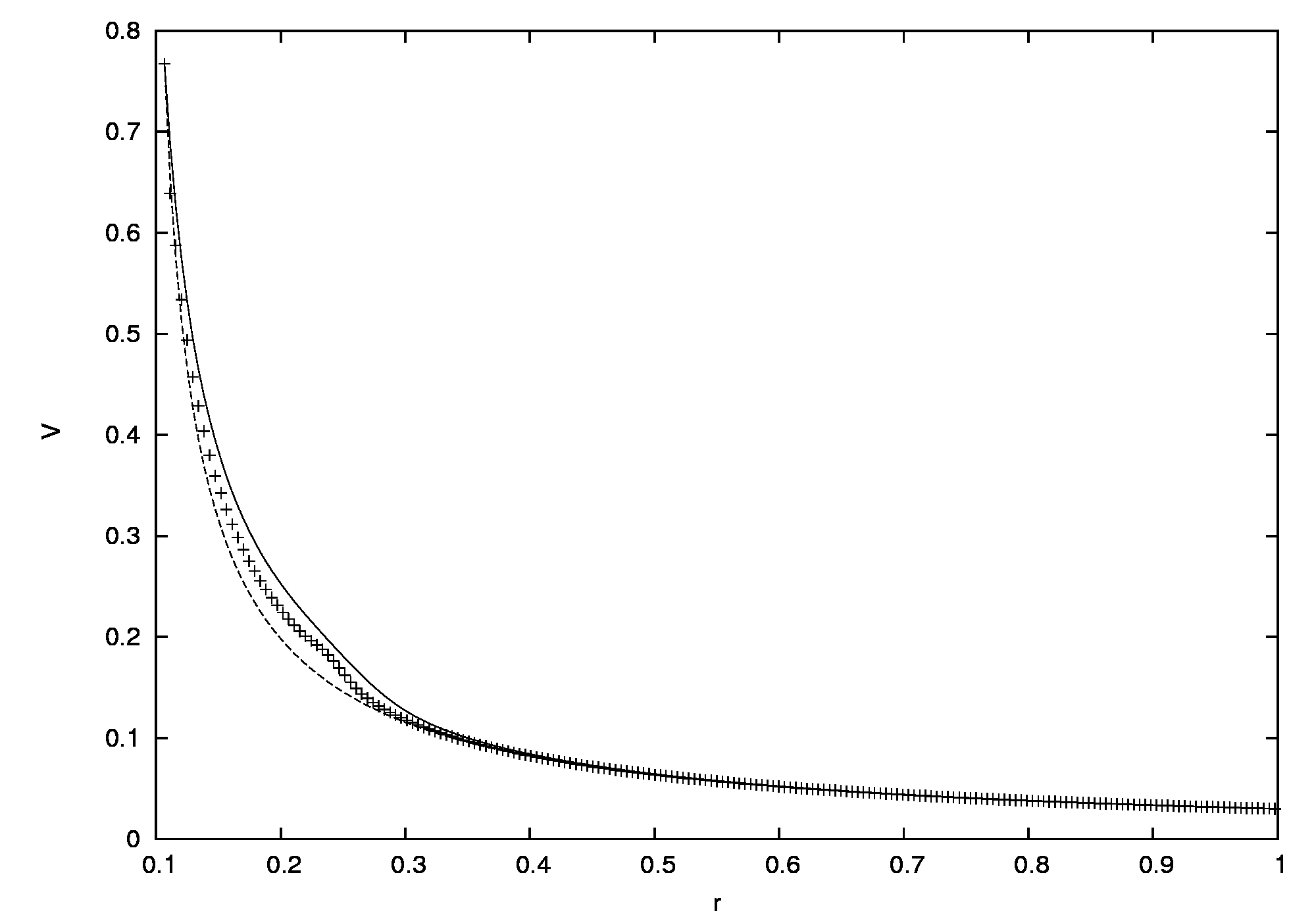
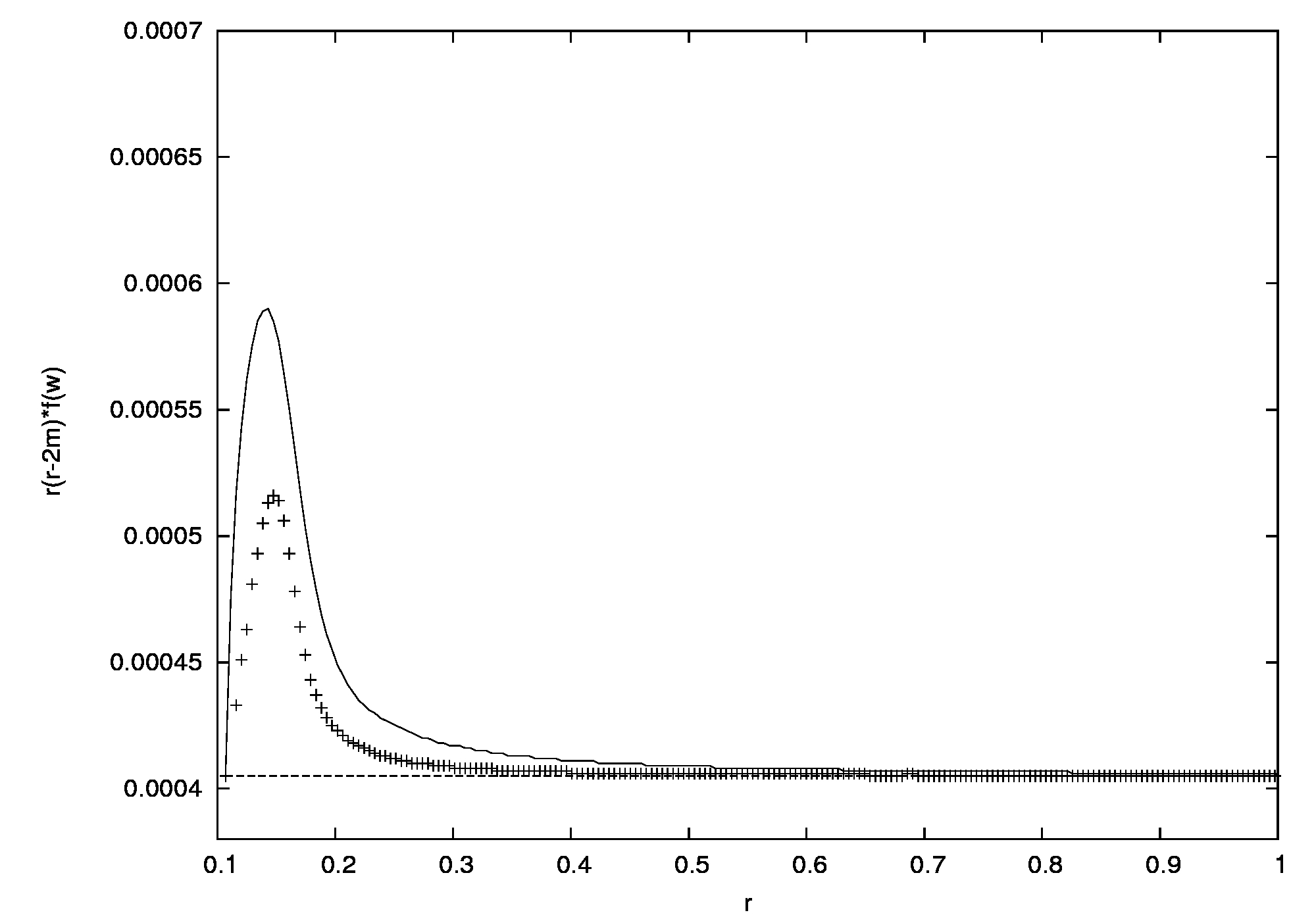
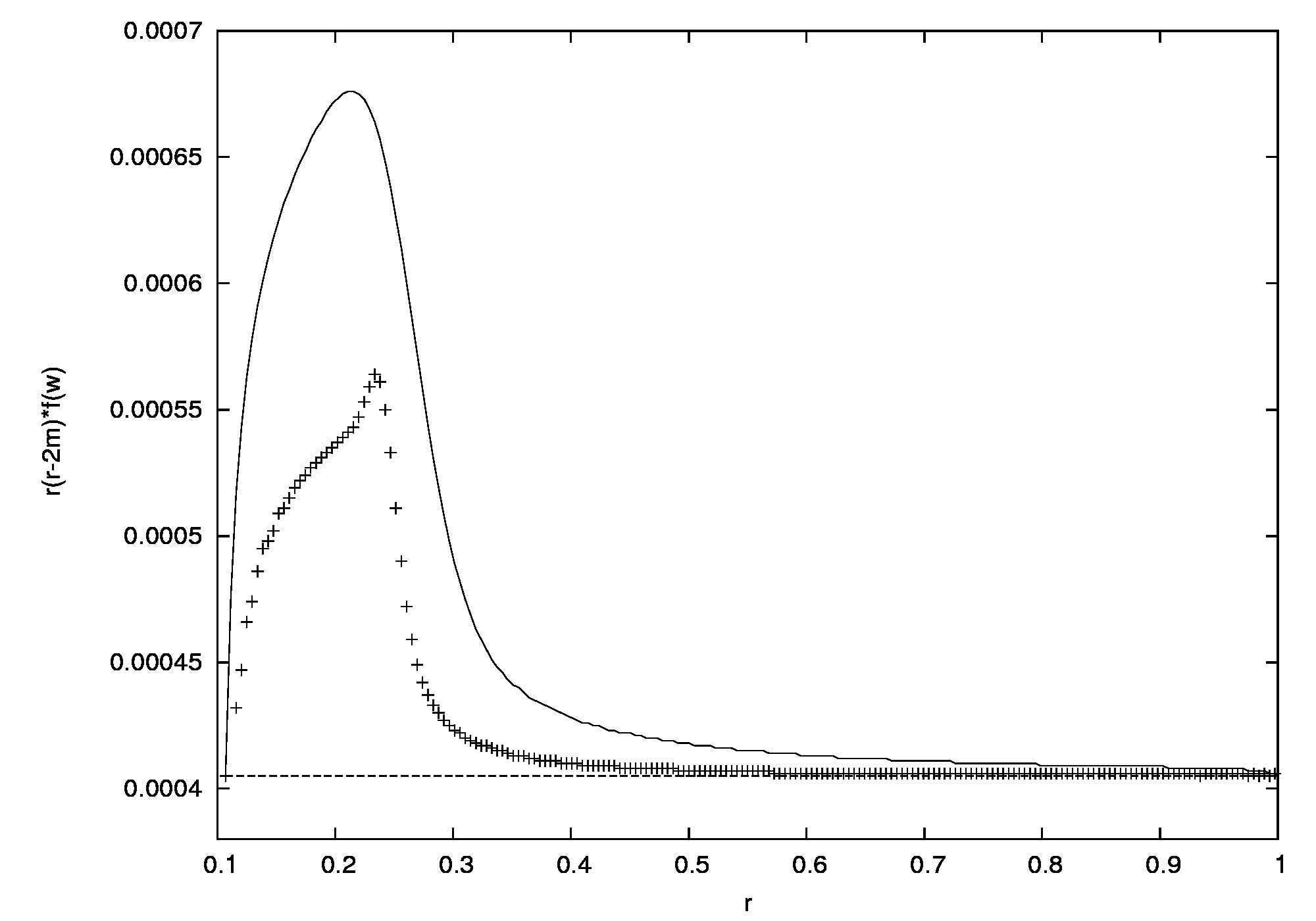
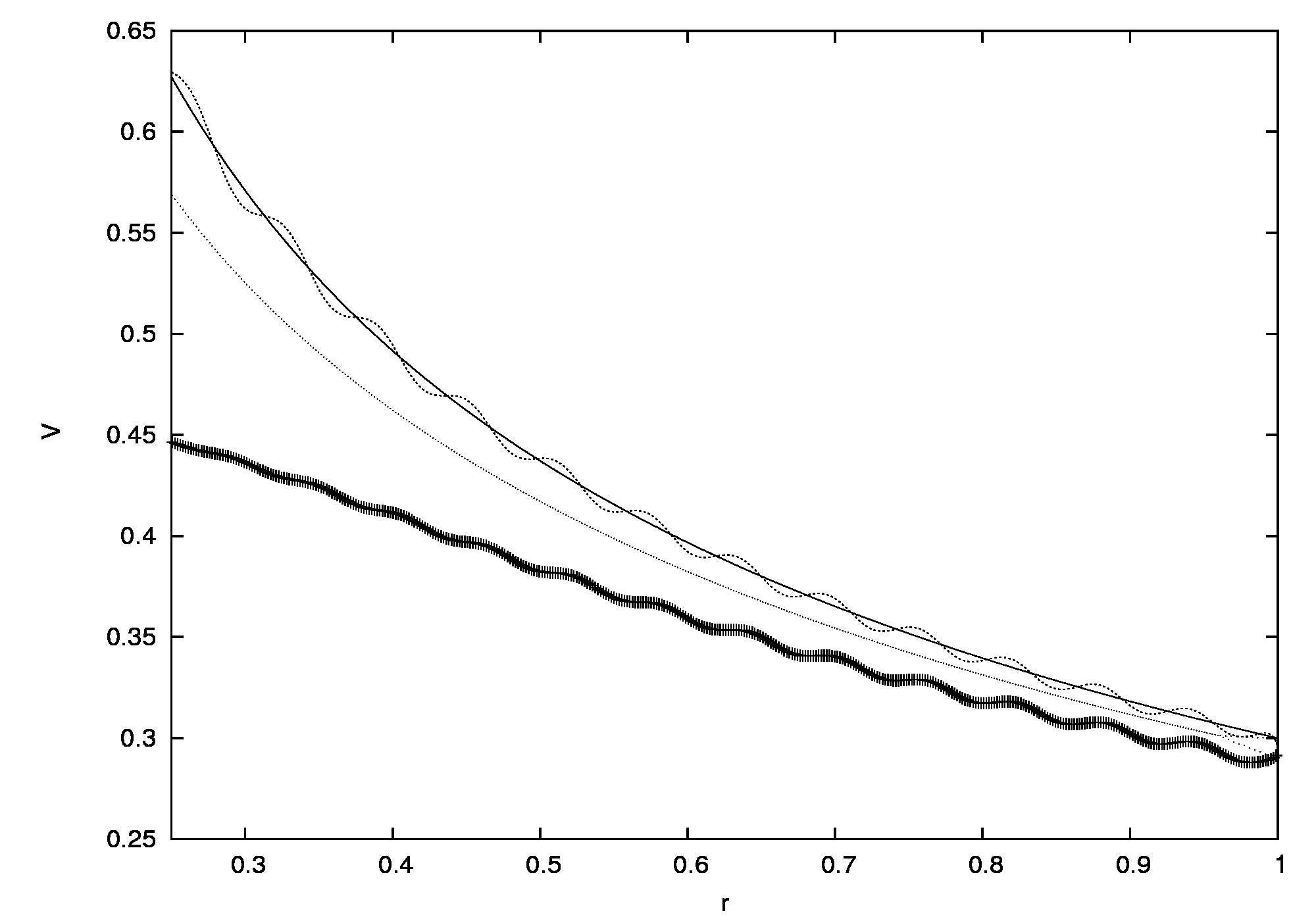
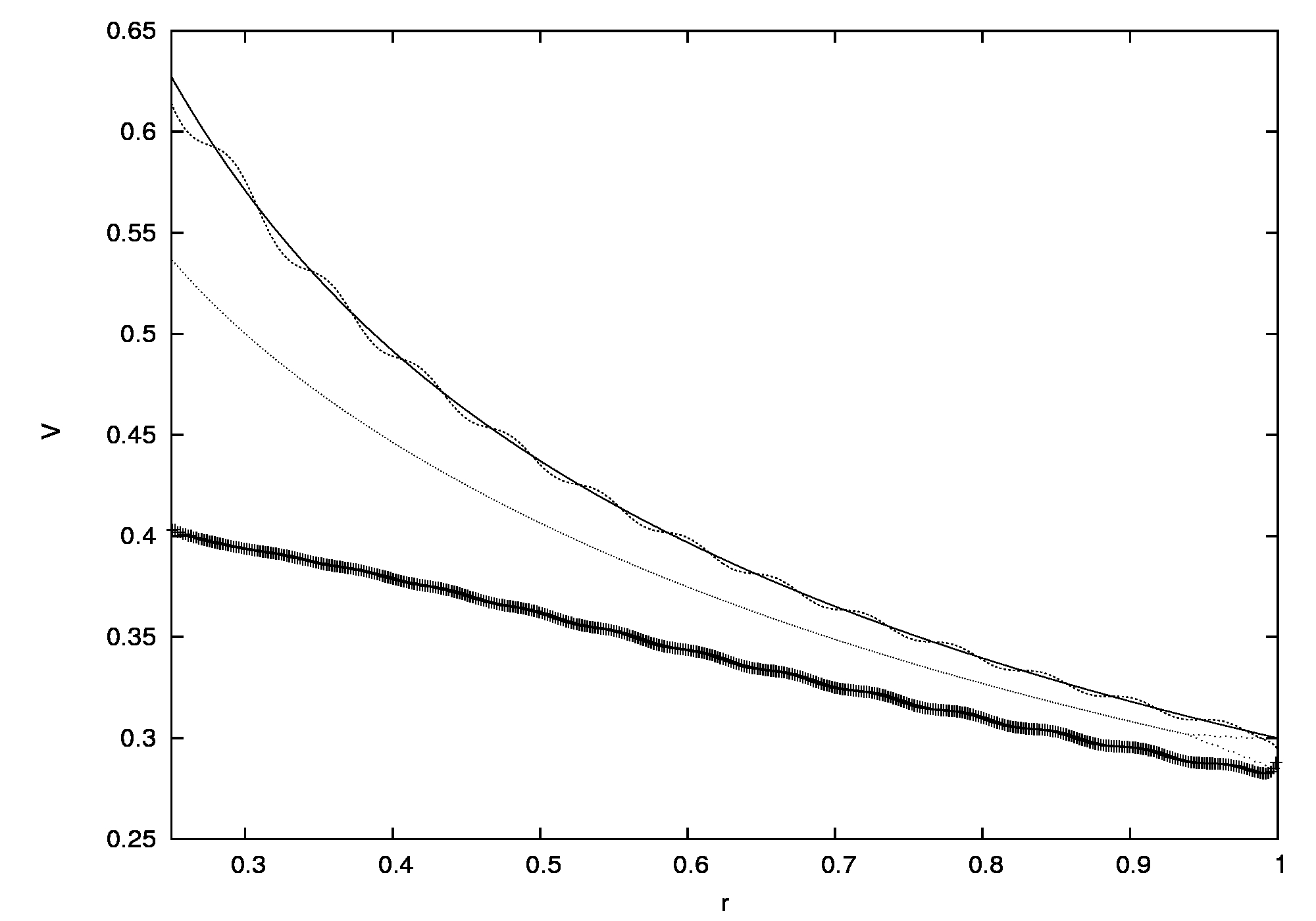
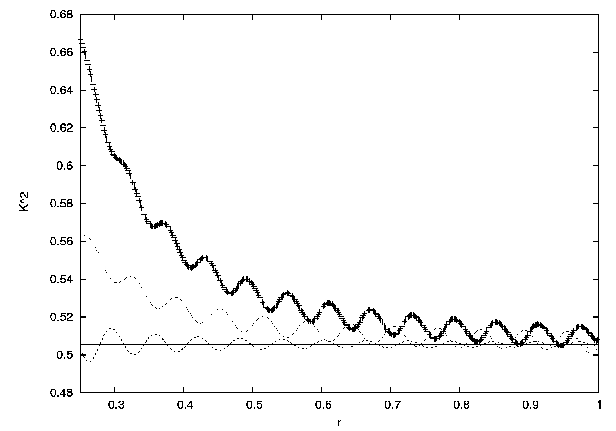
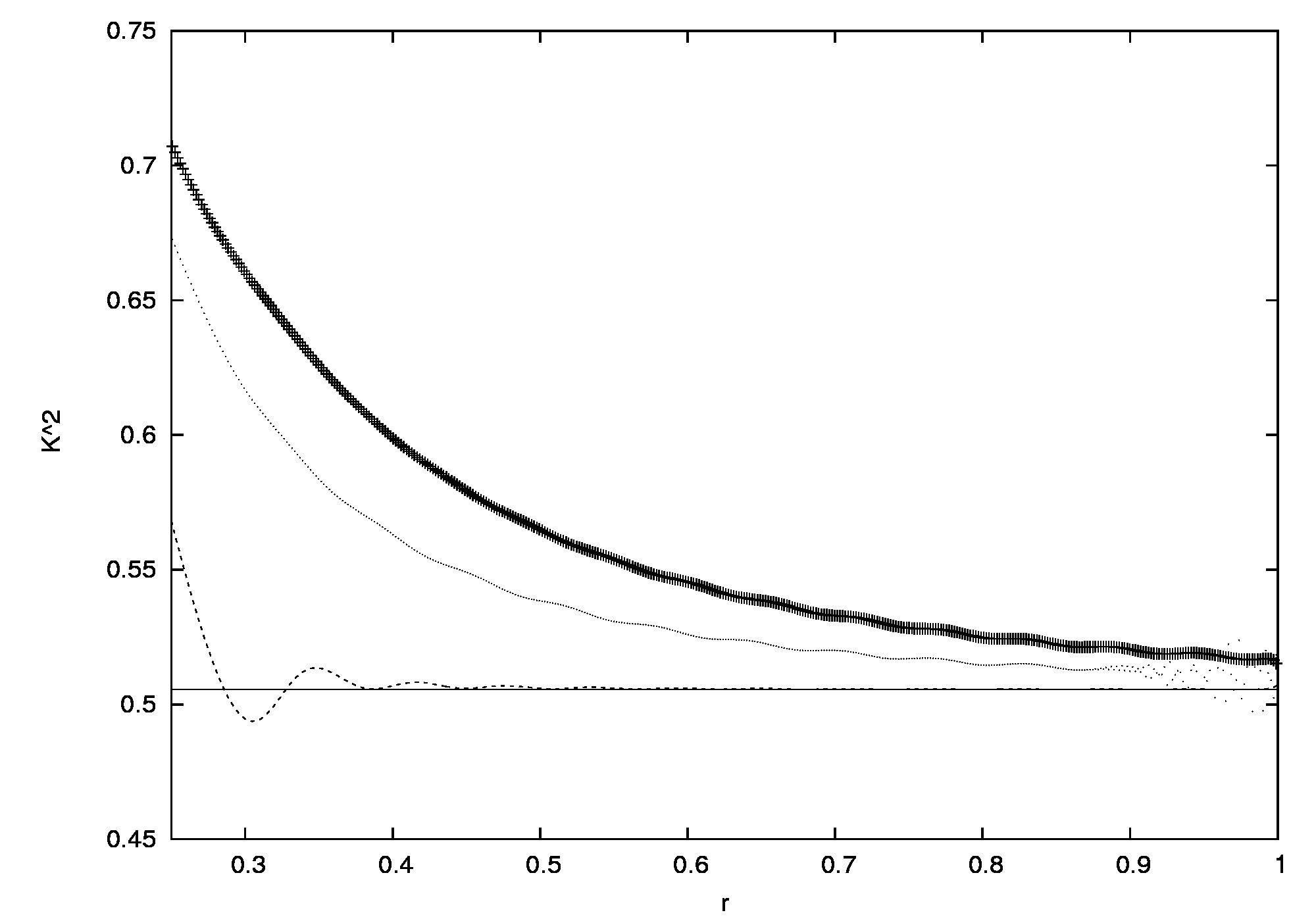
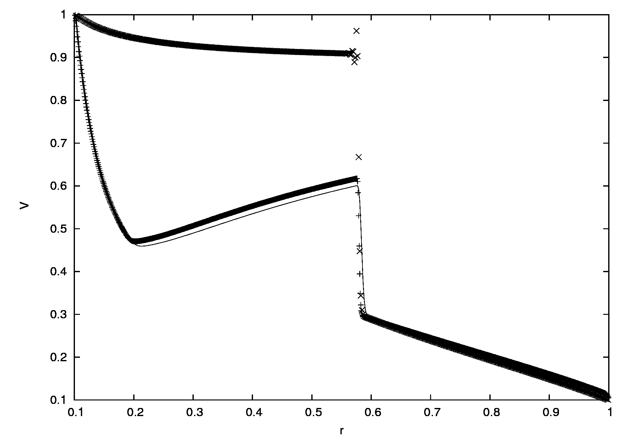
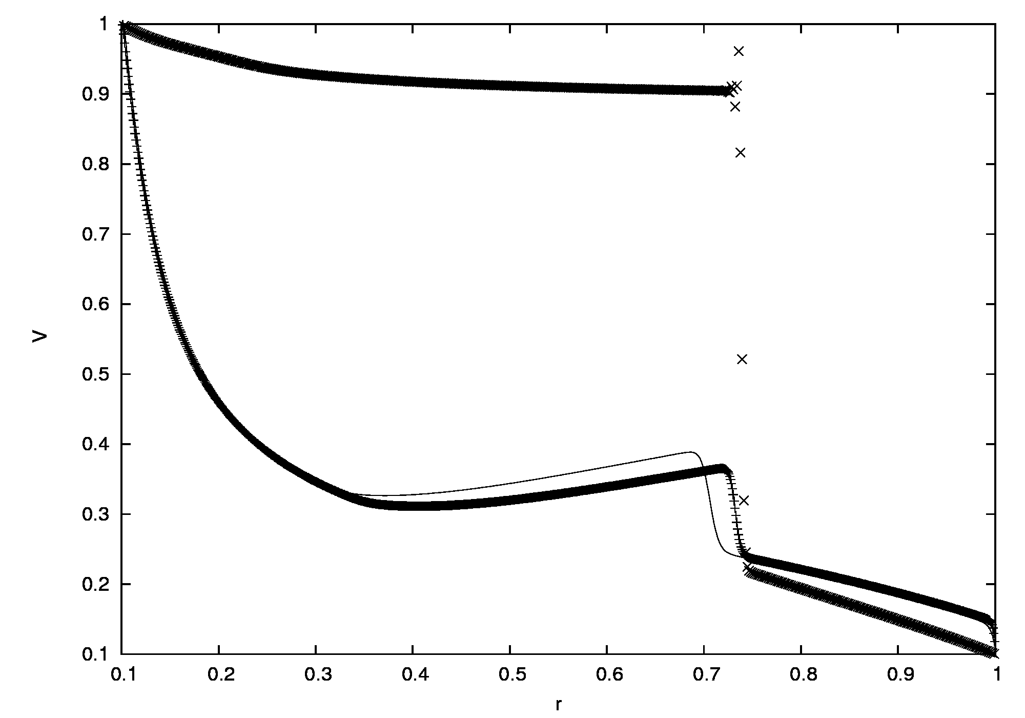
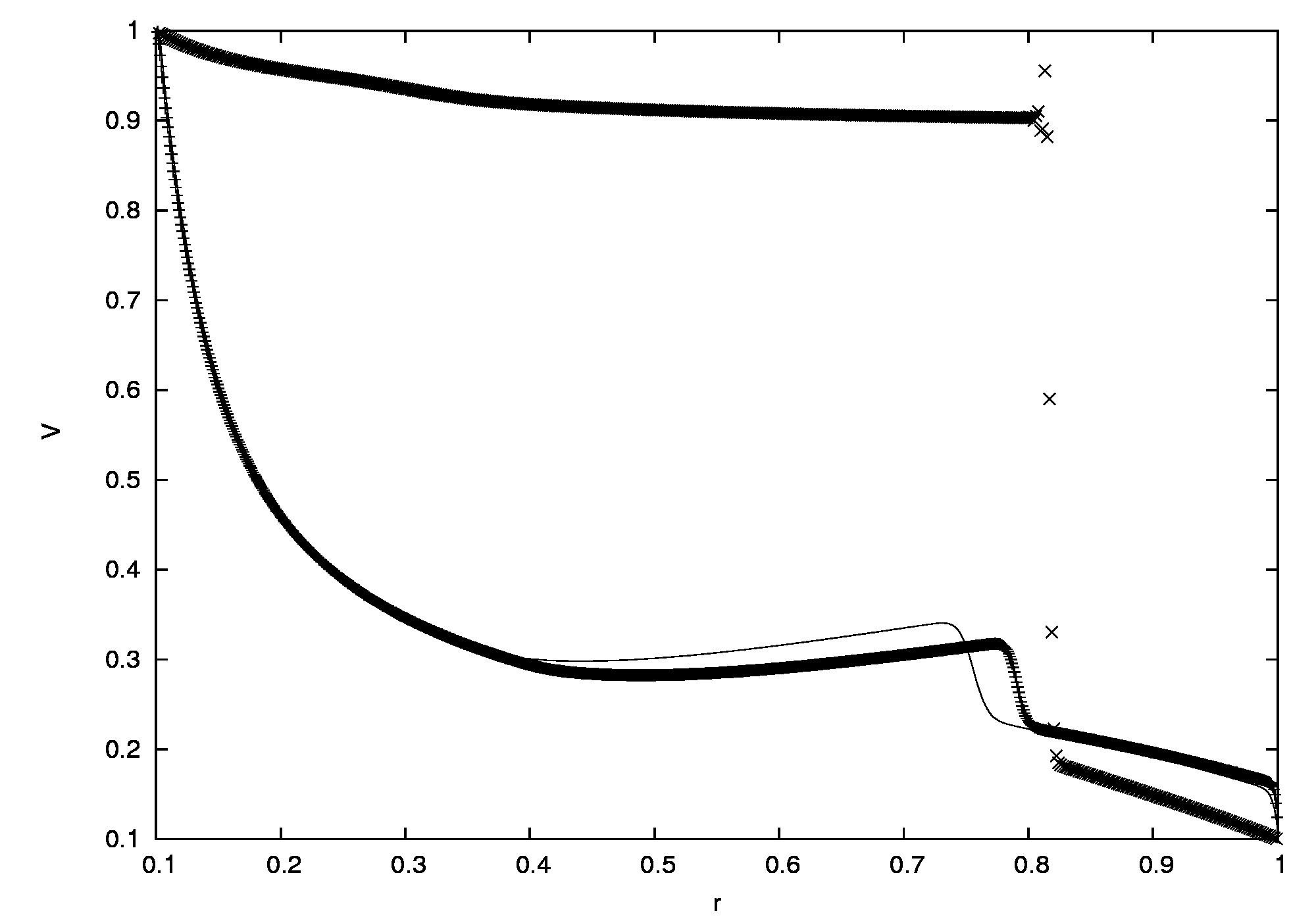
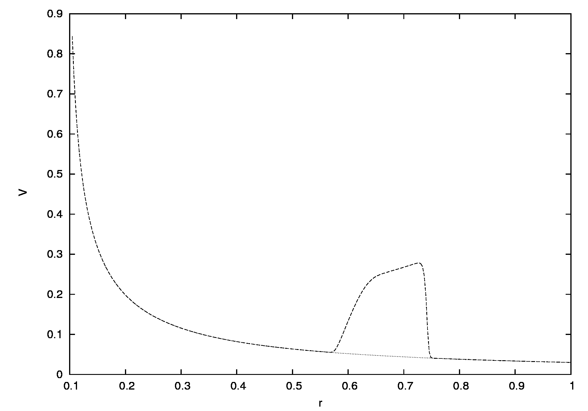
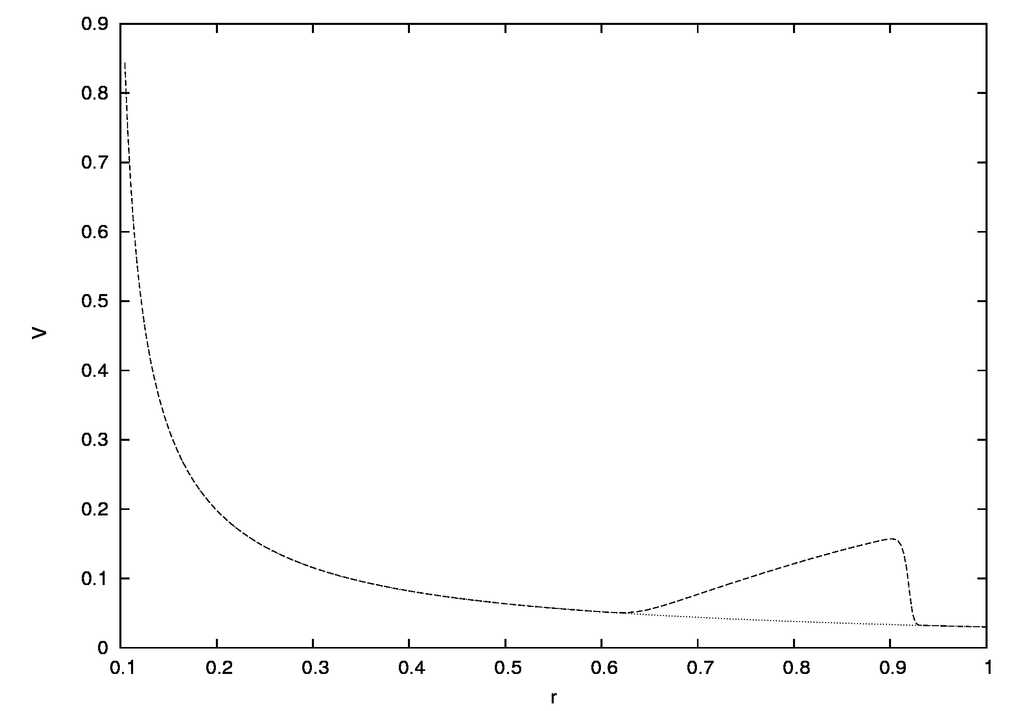
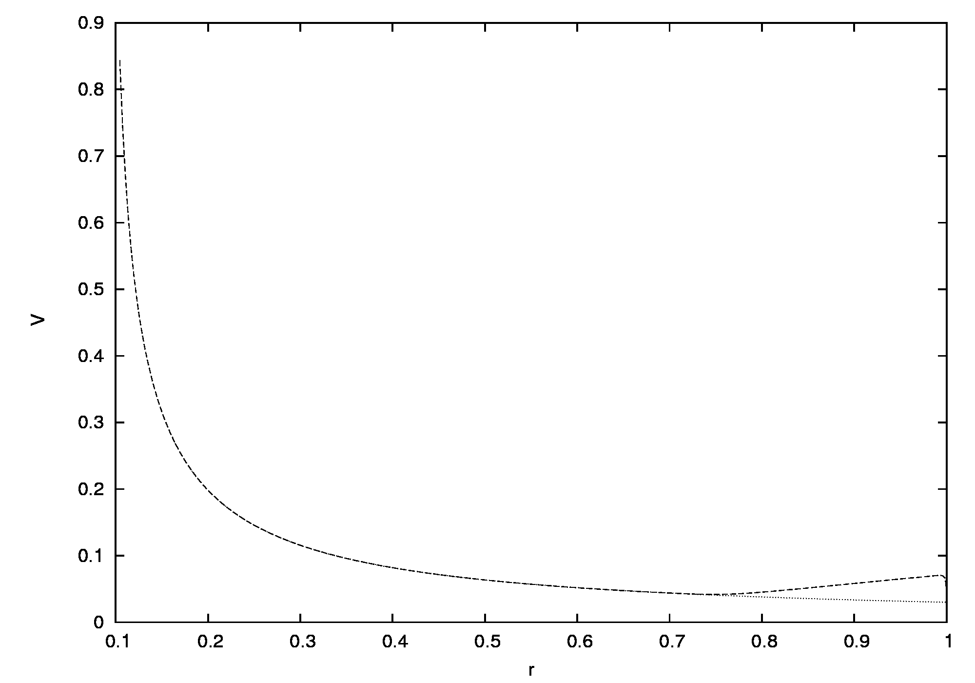
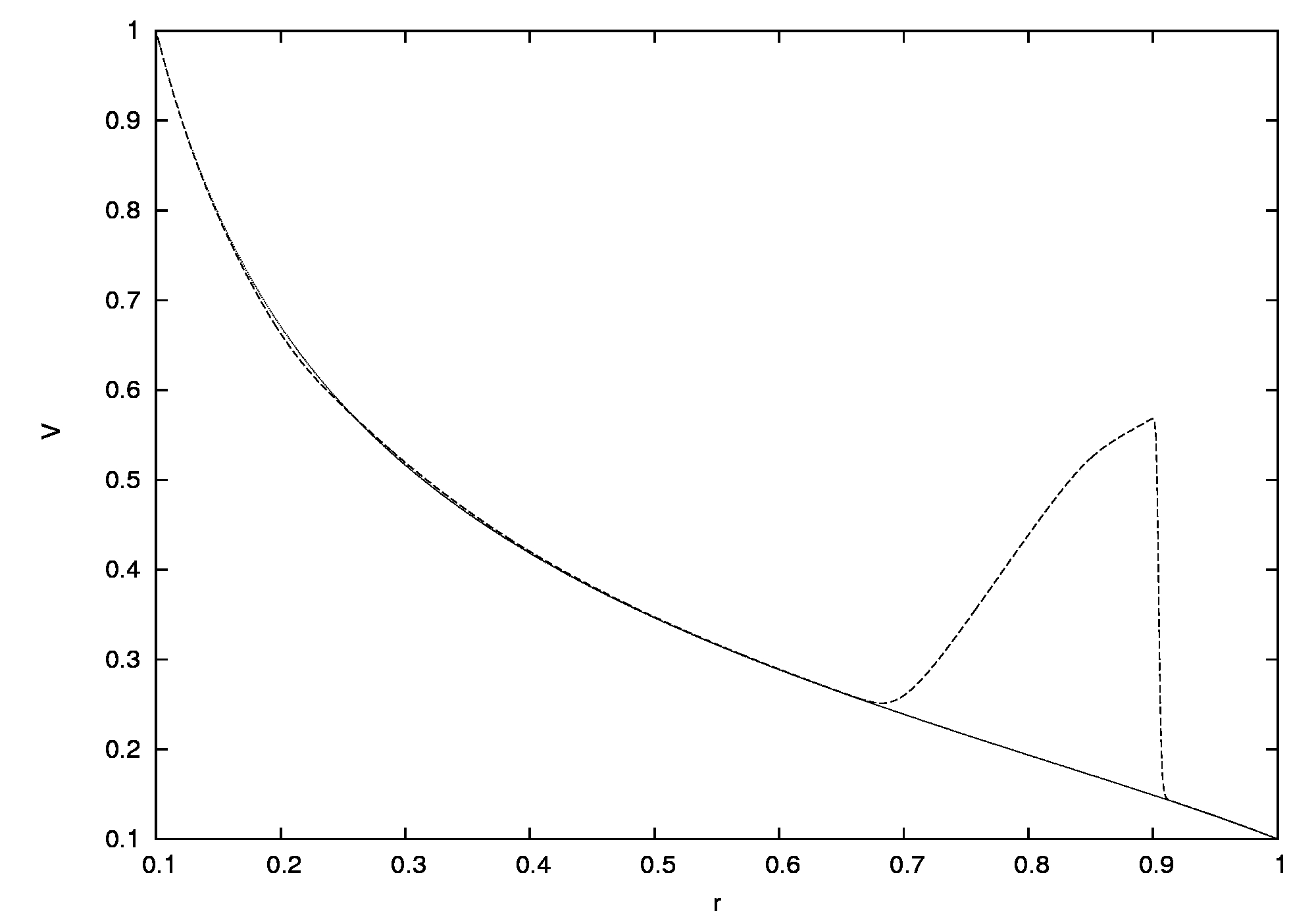
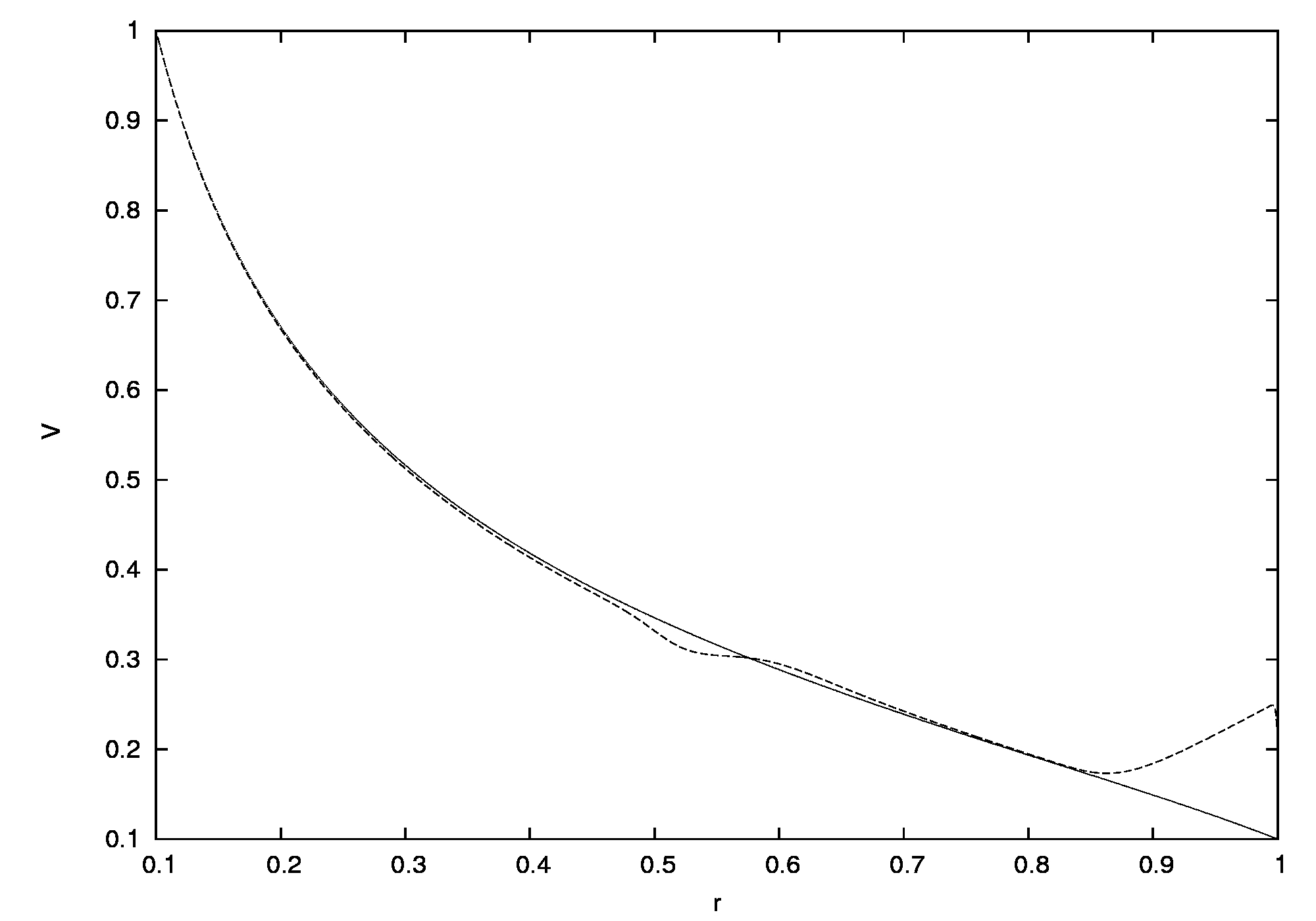
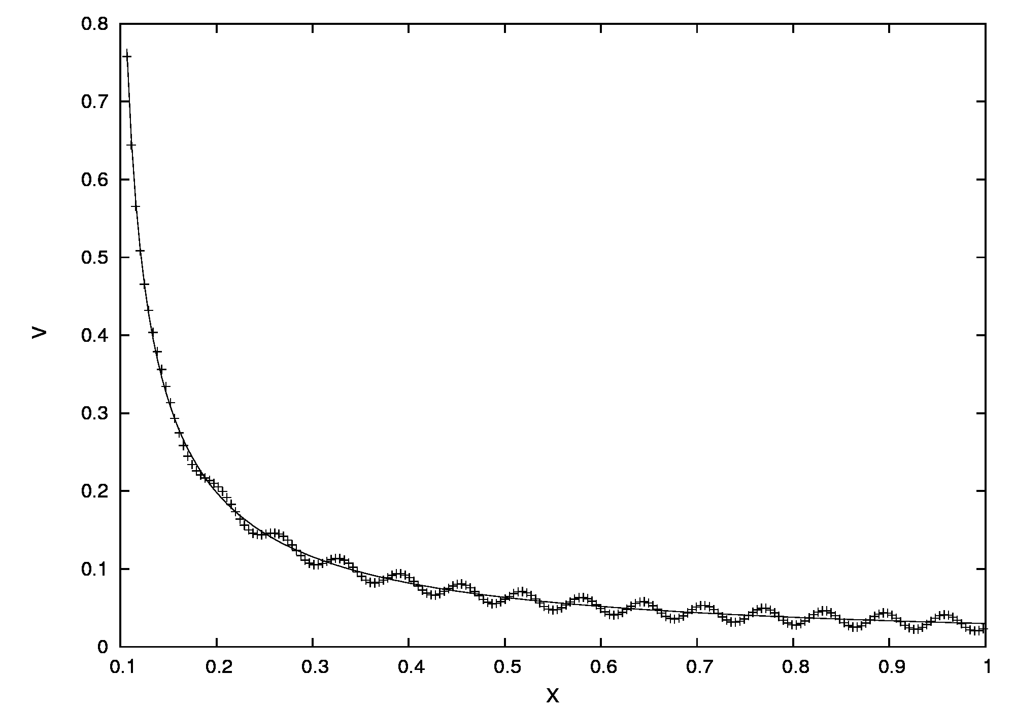
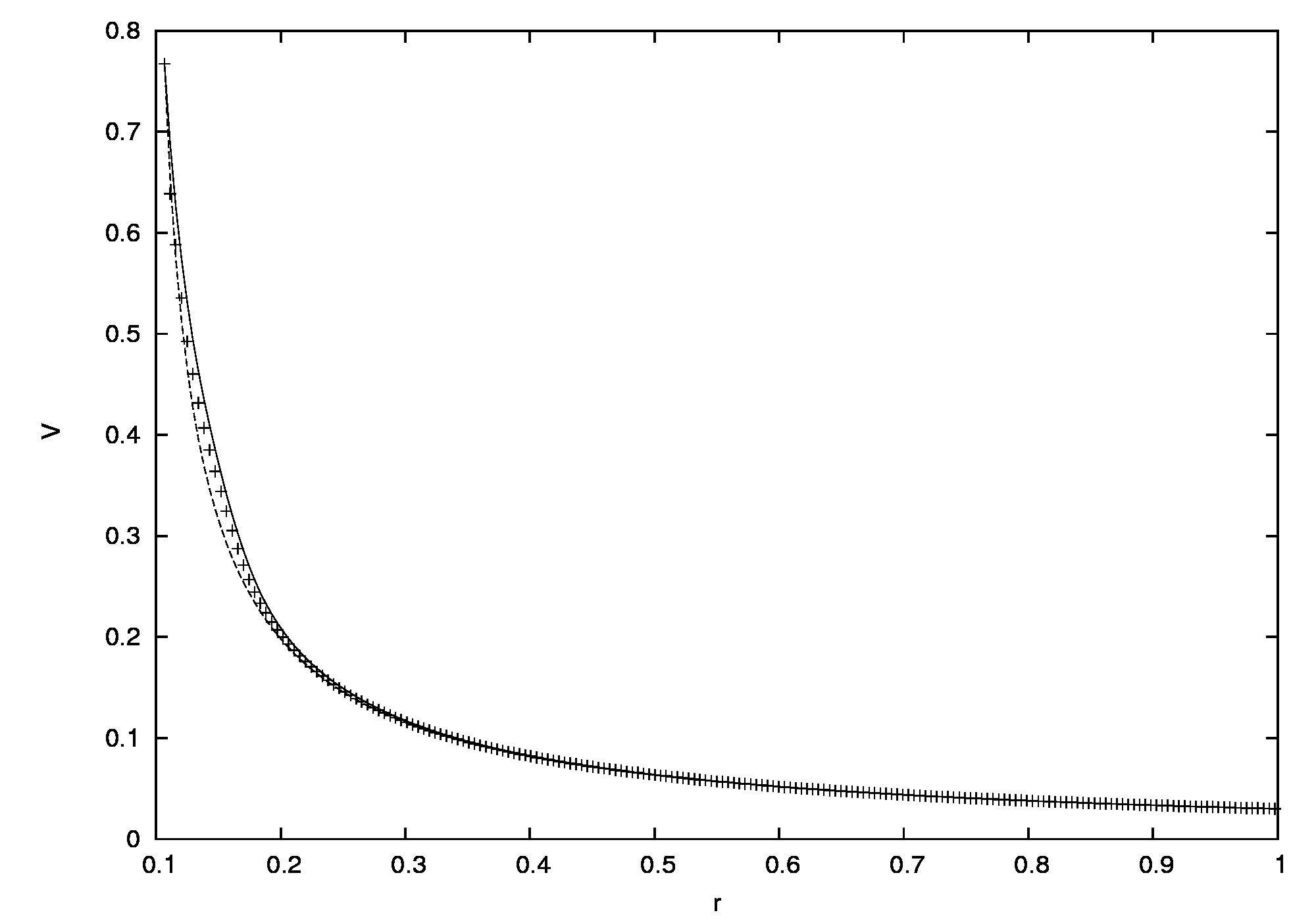
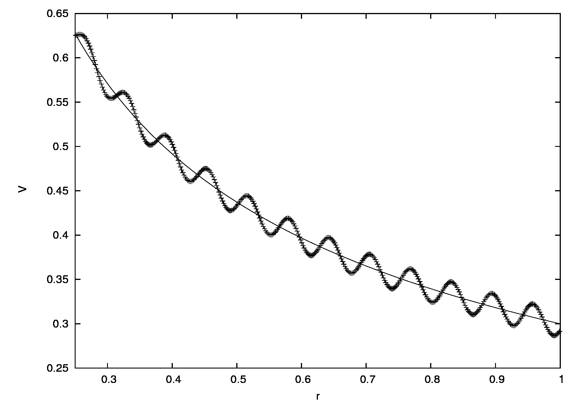
with obvious notation. The first equation has a conservative form, while the second one is nonconservative. We work within the interval r(2m,R)𝑟2𝑚𝑅r\in(2m,R), where R𝑅R is a fixed upper bound for the spatial variable. We impose no-influx boundary conditions at r=2m𝑟2𝑚r=2m and r=R𝑟𝑅r=R by solving a Riemann problem between the boundary data determined by the initial data and the current numerical value at the boundary. In other words, we use the Godunov flux at the boundary. For all numerical experiments, we use 2m=0.12𝑚0.12m=0.1 and R=1.0𝑅1.0R=1.0 and the value of CFL number is taken to be 0.90.90.9. We begin by illustrating the importance of the well balanced property by comparing together the numerical solutions obtained with the proposed scheme and with a more naive discretization of the right–hand side of the geometric Burgers equation (II). For the model (I), we used Δr=0.02Δ𝑟0.02\Delta r=0.02 and the endpoint velocity v(R)=0.03𝑣𝑅0.03v(R)=0.03. The numerical solution is plotted on Figure 5.1.1. In this Figure, in (b), (c), we plot the numerical solutions given by the three schemes. The first one is the first–order Lax–Friedrichs scheme (which is indicated by ++); the second one is the second–order version of Lax–Friedrichs scheme (which is indicated by line); the third one is the well balanced second–order version of Lax–Friedrichs scheme (which is indicated by -). In Figures (d), (e), we compare the numerical flux r(r2m)fϵ(w)𝑟𝑟2𝑚subscript𝑓italic-ϵ𝑤r(r-2m)\,f_{\epsilon}(w) (cf. (41)), by the three schemes. The proposed well balanced scheme appears to be efficient and robust and, in particular, this scheme preserves steady solutions. Next, for the model (II), we used Δr=0.005Δ𝑟0.005\Delta r=0.005 and the velocity v(R)=0.3𝑣𝑅0.3v(R)=0.3, which led us to Figure 5.1.2. In Figures (b) and (c), we compare the numerical solutions based on the three schemes. The first one is a standard first–order Lax–Friedrichs scheme (which is indicated by +); the second one is a standard second–order Lax–Friedrichs scheme (and is plotted with dots); the third one is a well balanced second–order Lax–Friedrichs scheme (and is plotted with -). In Figures (d) and (e), we compare the numerical values of K2superscript𝐾2K^{2} (defined in (29)) based on the three schemes. Again, the scheme is found to be efficient and preserve steady solutions.
Refer to caption
(a)
Refer to caption
(b)
Refer to caption
(c)
Refer to caption
(d)
Refer to caption
(e)

Figure 5.1.1. The numerical solutions given by the three schemes for the first model (I).
Refer to caption
(f)
Refer to caption
(g)
Refer to caption
(h)
Refer to caption
(i)
Refer to caption
(j)

Figure 5.1.2. The numerical solutions given by the three schemes for the second model (II).

5.2 Comparison of several schemes for a single shock
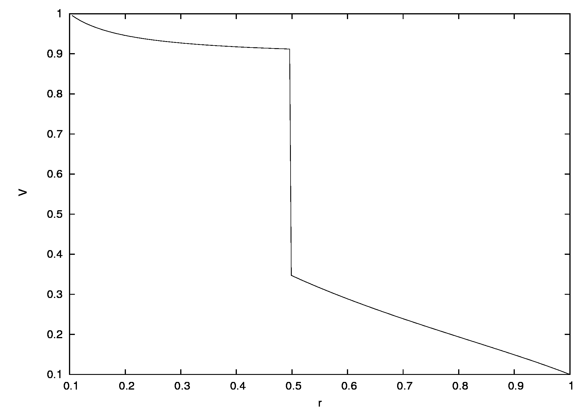
Refer to caption
(k)
Refer to caption
(l)
Refer to caption
(m)
Refer to caption
(n)

Figure 5.2. The numerical solutions given by the three schemes for the second model (II).

We study next weak solutions containing a single shock separating two steady solutions at the location r=0.5𝑟0.5r=0.5: one steady solution corresponds to the data v1(R)=0.1subscript𝑣1𝑅0.1v_{1}(R)=0.1 while the other steady solution corresponds to v2(R)=0.9subscript𝑣2𝑅0.9v_{2}(R)=0.9. The initial data are constructed so that the initial discontinuity propagates as a single shock (without decomposing itself during the evolution), which interacts with the background geometry. We consider the second model (42) with Δr=0.05Δ𝑟0.05\Delta r=0.05 . The numerical solution is presented in Figure 5.2. We compare the propagation of a single shock by three schemes. The first one is a standard first–order Lax–Friedrichs scheme (plotted with a continuous line), and the second one is a standard second–order Lax–Friedrichs scheme (ploted with the symbol ++). Finally, the third scheme is the proposed well balanced second–order Lax–Friedrichs scheme (plotted with the symbol ×\times). One observes the efficiency and robustness of the well balanced scheme; the numerical solution based on this scheme is monotone and stable under perturbations.

5.3 Application to late-time asymptotics – perturbed steady solutions
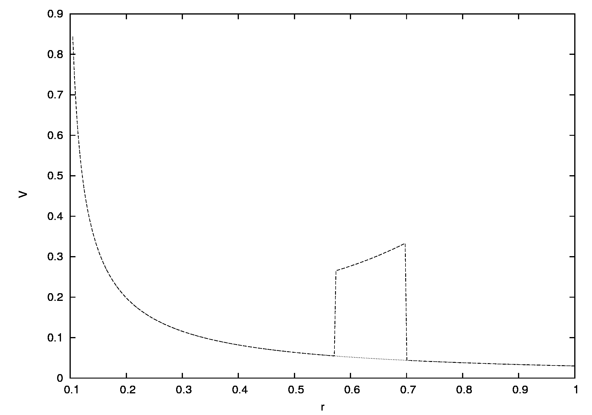
Refer to caption
(o)
Refer to caption
(p)
Refer to caption
(q)
Refer to caption
(r)

Figure 5.3.1. Model (I). The asymptotic behaviors of long time solutions for equation (41) using the well balanced second–order scheme.

We study here the nonlinear stability of a steady solution superimposed with a compactly supported initial perturbation. In Figure 5.3.1, we still use (41) and take each subinterval Δr=0.03Δ𝑟0.03\Delta r=0.03 and a velocity at the right-hand point v(R)=0.03𝑣𝑅0.03v(R)=0.03. We observe that the initial perturbation evolves toward a so-called N𝑁N–wave, which is typical of nonlinear hyperbolic systems, and that this perturbation moves in the right direction away from the singularity. It eventually goes away at the boundary r=R𝑟𝑅r=R of the computational domain. We observe the convergence of the solution toward the steady solution using the well balanced second–order Lax–Friedrichs scheme. One observes that the numerical solution, using the well balanced second–order Lax–Friedrichs scheme, is stable. Next, in Figure 5.3.2, we treated the second model (42), with Δr=0.001Δ𝑟0.001\Delta r=0.001 and v(R)=0.1𝑣𝑅0.1v(R)=0.1, and similarly to the first case, one observes that the initial perturbation evolves toward a so–called N𝑁N–wave, and that this perturbation moves in the right direction away from the singularity. Again, the solution converges toward the steady solution.
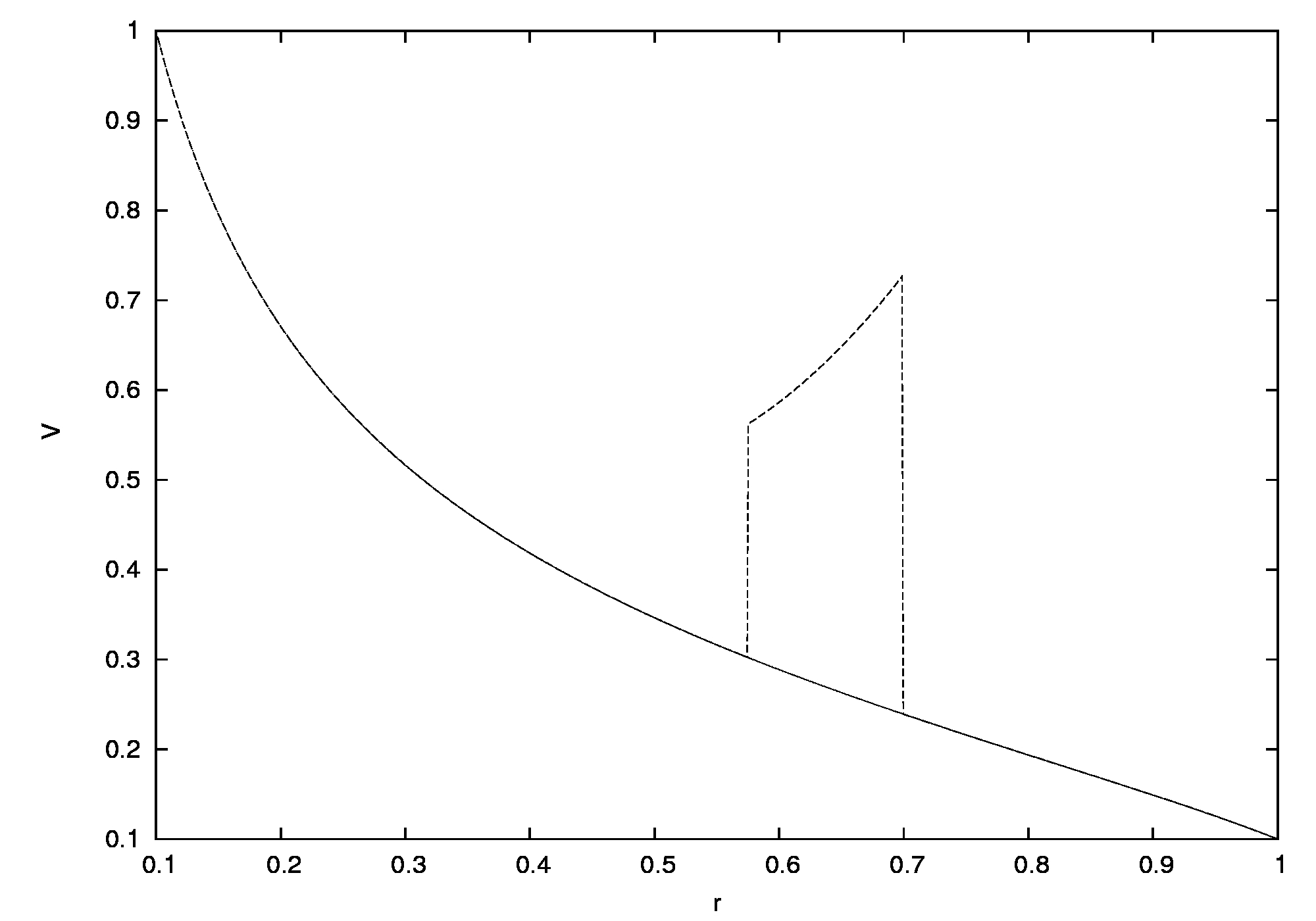
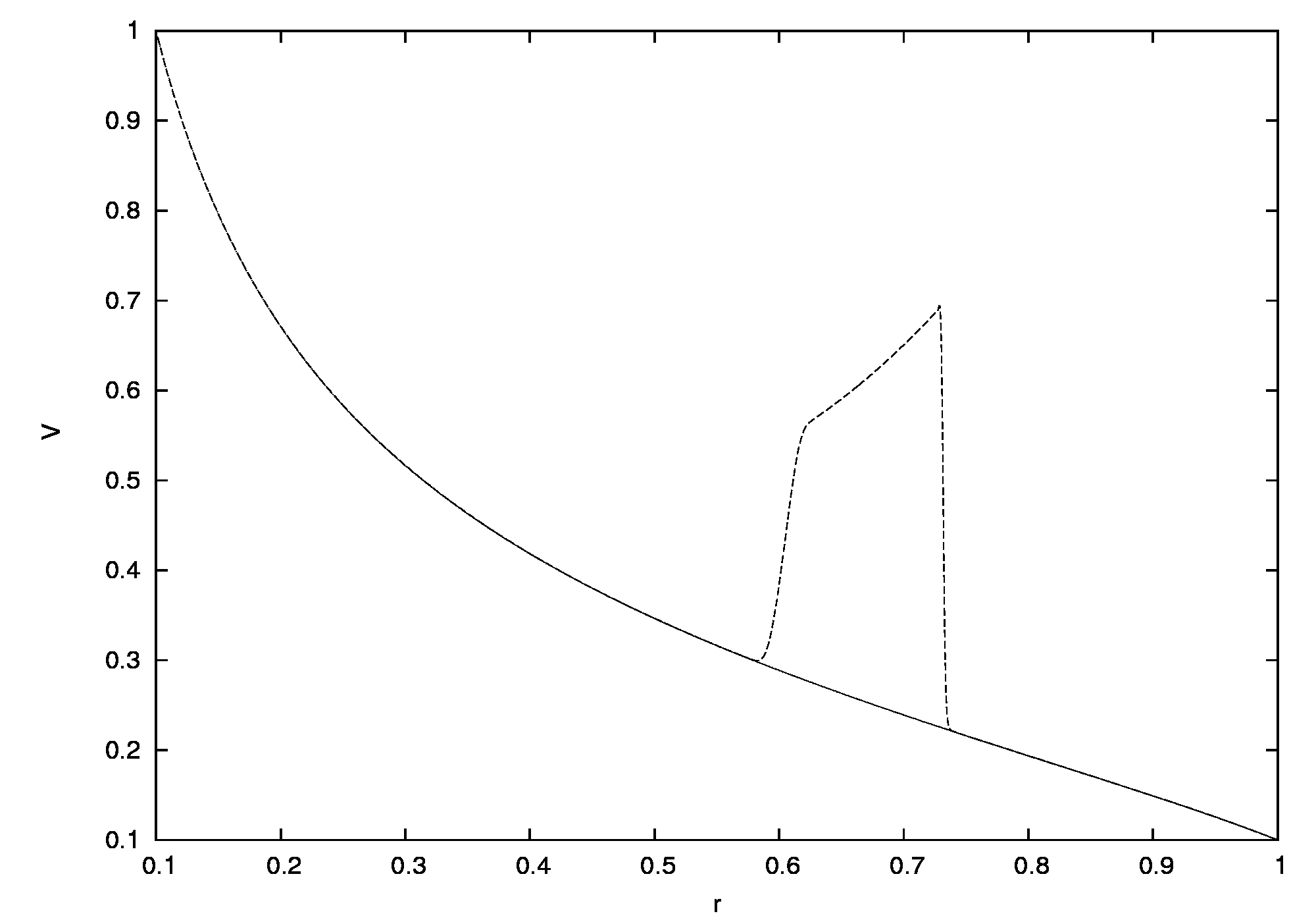
Refer to caption
(s)
Refer to caption
(t)
Refer to caption
(u)
Refer to caption
(v)

Figure 5.3.2. Model (II). Late-time asymptotic behavior for the model (42) using the well balanced second–order scheme.

5.4 Application to late-time asymptotics – perturbed one shock solution

Finally, we take the case of a solution containing a single steady shock separating two initially steady solutions for the equation (33) at the location r=0.5𝑟0.5r=0.5. We consider here the first model (41) with Δr=0.05Δ𝑟0.05\Delta r=0.05 and v(R)=0.09𝑣𝑅0.09v(R)=0.09. We study here the nonlinear stability of this steady solution and include initial perturbation on a steady solution. The numerical results are plotted in Figure 5.4. We observe the convergence of the solution toward the steady solution (single steady shock) using the well balanced second–order Lax–Friedrichs scheme.

6 Conclusions

In the first part of this paper, we considered a general class of hyperbolic balance laws posed on a curved spacetimes and we derived flux vector fields T=T(v)𝑇𝑇𝑣T=T(v) which, in a relativistic context, generalize the classical Burgers flux. On one hand, we required that (1) satisfies the Lorentz invariance property shared by the Euler equations of relativistic compressible fluids, and we identified a balance law, which is unique up to normalization. Interestingly enough, the standard Burgers equation was recovered by taking the singular limit of infinite light speed. On the other hand, an alternative model of interest was derived directly from the relativistic Euler equations, by assuming that the pressure term vanishes. This latter model, in the case of a flat background geometry, turned out to be simply the classical Burgers equation. Both models are referred to relativistic Burgers equations on curved spacetimes. They exhibit many of the mathematical properties (hyperbolicity, genuine nonlinearity, steady solutions) and challenges (shock wave, late-time asymptotics) encountered with the Euler system of relativistic compressible fluids. In the second part of this paper, we investigated the numerical discretization of entropy solutions to the above two models. We introduced a finite volume scheme for (1) defined on curved spacetimes, especially on a background Schwarzschild spacetime. The proposed scheme is fully consistent with the divergence form of the equations and, therefore, applies to weak solutions containing shock waves. More importantly, our scheme is well balanced in the sense that it preserves steady solutions, and extensive numerical experiments demonstrated the convergence of the proposed scheme, and its relevance for computing entropy solutions on a curved background. The generalization to the Euler equations posed on Schwarzschild spacetime are presented in the follow-up work [6].

References

  • [1] P. Amorim, P.G. LeFloch, and B. Okutmustur, Finite volume schemes on Lorentzian manifolds, Commun. Math. Sci. 6 (2008), 1059–1086.
  • [2] M. Ben-Artzi and P.G. LeFloch, The well posedness theory for geometry compatible hyperbolic conservation laws on manifolds, Ann. Inst. H. Poincaré Anal. Non Linéaire 24 (2007), 989–-1008.
  • [3] F. Bouchut, Nonlinear stability of finite volume methods for hyperbolic conservation laws and well balanced schemes for sources, Birkhäuser, Verlag, Bäsel, 2004.
  • [4] J.M. Greenberg and A.Y. Leroux, A well balanced scheme for the numerical processing of source terms in hyperbolic equations, SIAM J. Numer. Anal. 33 (1996), 1–16.
  • [5] P.G. LeFloch, Hyperbolic conservation laws on spacetimes, in “Nonlinear conservation laws and applications”, IMA Vol. Math. Appl. 153, Springer, New York, 2011, pp.  379–-391.
  • [6] P.G. LeFloch and H. Makhlof, A well–balanced finite volume method for compressible fluid flows on Schwarzschild spacetime, Preprint 2012.
  • [7] P.G. LeFloch and B. Okutmustur, Hyperbolic conservation laws on spacetimes. A finite volume scheme based on differential forms, Far East J. Math. Sci. 31 (2008), 49–83.
  • [8] R.J. LeVeque, Balancing source terms and flux gradients in high-resolution Godunov methods: The quasi-steady wave-propagation algorithm, J. Comput. Phys (1998), 346–365.
  • [9] H. Nessyahu and E. Tadmor, Nonoscillatory central differencing for hyperbolic conservation laws, J. Comput. Phys. 87 2 (1990), 408–463.
  • [10] G. Puppo and G. Russo, Staggered finite difference schemes for conservation laws, J. Sci. Comput. 27 (2006), 403–418.
  • [11] G. Russo, Central schemes for conservation laws with application to shallow water equations, S. Rionero and G. Romano Editors, Trends Appl. Math. Mech., STAMM 2002, Springer Verlag, Italia SRL 2005, pp. 225–246.
  • [12] G. Russo, High-order shock-capturing schemes for balance laws, in “Numerical solutions of partial differential equations”, Adv. Course Math. CRM Barcelona, Birkhäuser, Basel, 2009, pp. 59–147.
  • [13] G. Russo and A. Khe, High–order well balanced schemes for systems of balance laws, in “Hyperbolic problems: theory, numerics and applications”, Proc. Sympos. Appl. Math., Vol. 67, Part 2, Amer. Math. Soc., Providence, RI, 2009, pp. 919–928.