On Constrained Randomized Quantization

Abstract

Randomized (dithered) quantization is a method capable of achieving white reconstruction error independent of the source. Dithered quantizers have traditionally been considered within their natural setting of uniform quantization. In this paper we extend conventional dithered quantization to nonuniform quantization, via a subterfage: dithering is performed in the companded domain. Closed form necessary conditions for optimality of the compressor and expander mappings are derived for both fixed and variable rate randomized quantization. Numerically, mappings are optimized by iteratively imposing these necessary conditions. The framework is extended to include an explicit constraint that deterministic or randomized quantizers yield reconstruction error that is uncorrelated with the source. Surprising theoretical results show direct and simple connection between the optimal constrained quantizers and their unconstrained counterparts. Numerical results for the Gaussian source provide strong evidence that the proposed constrained randomized quantizer outperforms the conventional dithered quantizer, as well as the constrained deterministic quantizer. Moreover, the proposed constrained quantizer renders the reconstruction error nearly white. In the second part of the paper, we investigate whether uncorrelated reconstruction error requires random coding to achieve asymptotic optimality. We show that for a Gaussian source, the optimal vector quantizer of asymptotically high dimension whose quantization error is uncorrelated with the source, is indeed random. Thus, random encoding in this setting of rate-distortion theory, is not merely a tool to characterize performance bounds, but a required property of quantizers that approach such bounds.

I Introduction

Dithered quantization is a randomized quantization method introduced in [roberts1962picture]. A central motivation for dithered quantization is its ability to yield quantization error that is independent of the source, which can be achieved if certain conditions, determined by Schuchman, are met [Schuchman]. Traditionally, dithered quantization has been studied in the framework where the quantizer is uniform (with step size $\Delta$) and the dither signal is uniformly distributed over $(-\frac{\Delta}{2},\frac{\Delta}{2})$, matched to the quantizer interval as shown in Figure 1. A uniformly distributed dither signal is added before quantization and the same dither signal is subtracted from the quantized value at the decoder side. Note that only subtractive dithering is considered in this paper. In the variable rate case, the quantized values are entropy coded, conditioned on the dither signal. Randomized (dithered) quantizers have been studied in the past due to important properties that differentiate them from deterministic quantizers, and were employed to characterize rate-distortion bounds for universal compression [ziv_quantization, graydq]. Zamir and Feder provide extensive studies of the properties of dithered quantizers [zamiruqr, zamirirp].

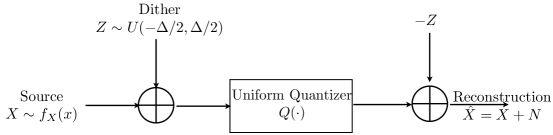
Figure 1: The basic structure of dithered quantization

Beyond its theoretical significance, randomized quantization is of practical interest. Many filter/system optimization problems in practical compression settings, such as the “rate-distortion optimal filterbank design” problem [mihcak], or low rate filter optimization for DPCM compression of Gaussian auto-regressive processes [guleryuz], assume quantization noise that is independent of (or uncorrrelated with) the source. Although this assumption is satisfied at asymptotically high rates [gershobook], such systems are mostly useful for very low rate applications. For example, in [guleryuz], it is stated that the assumptions made in the paper are not satisfied by deterministic quantizers, and that dithered quantizers satisfy the assumptions exactly. However, conventional (uniform) dithered quantization suffers from suboptimal compression performance. Hence, a quantizer that mostly satisfies the assumptions, but at minimal cost in performance degradation, would have considerable impact on many such applications.

In this paper, we consider a generalization to enable effective dithering of nonuniform quantizers. To the best of our knowledge, this paper is the first attempt (other than our preliminary work in [akyol2009nonuniform, akyoltowards]) to consider dithered quantization in a nonuniform quantization framework. One immediate problem with nonuniform dithered quantization is how to apply dithering to unequal quantization intervals. In traditional dithered quantization, the dither signal is matched to the uniform quantization interval while maintaining independence of the source, but it is not clear how to match the generic dither to varying quantization intervals. As a remedy to this problem, we propose dithering in the companded domain. We derive the closed form necessary conditions for optimality of the compressor and expander mappings for both fixed and variable rate randomized quantization. We numerically optimize the mappings by iteratively imposing these necessary conditions.

However, the resulting (unconstrained randomized) quantizer does not render reconstruction error orthogonal to the source. Therefore, we extend the framework to include an explicit such constraint. Surprising theoretical results show direct and simple connections between the optimally constrained random quantizers and their unconstrained counterparts. We note in passing that the nonuniform dithered quantizer subsumes the conventional uniform dithered quantizer as an extreme special case.

For the variable rate case, the proposed nonuniform dithered quantizer is expected to outperform the conventional dithered quantizer, most significantly at low rates where the optimal variable rate (entropy coded) quantizer is often far from uniform. We observe that a deterministic quantizer cannot render the quantization noise independent of the source but can make it uncorrelated with the source. We hence also present an alternative deterministic quantizer that provides quantization noise uncorrelated with the source. We derive the optimality conditions of such constrained quantizers, for both fixed and variable rate quantization, and compare their rate-distortion performance to that of randomized quantizers.

Dithered quantization offers an interesting theoretical twist. Randomized quantization is an instance of the random encoding principle used to elegantly prove the achievability of coding bounds in rate distortion theory [coverbook]. However, to actually achieve those bounds, a random encoding scheme is not necessary, as they can be approached by a sequence of deterministic quantizers of increasing block length. In the second part of the paper, we investigate the settings under which randomized quantization is asymptotically necessary. A trivial example involves requiring source-independent quantization error. It is obvious that the reconstruction (hence quantization error) is a deterministic function of the source when the quantizer is deterministic [gershobook], while conventional dithered quantization produces quantization error that is independent of the source. Although a deterministic quantizer can never render the quantization error independent of the source, it can produce quantization error uncorrelated with the source. A natural question is whether the rate distortion bound, subject to the uncorrelated error constraint, can be achieved (asymptotically) with a deterministic quantizer.

The paper is organized as follows: In Section III, we present the proposed nonuniform randomized quantizers, along with its extension to constrained randomized quantizer that renders the quantization error orthogonal to the source. In Section IV, we derive the necessary conditions of optimality for the deterministic quantizer that generates reconstruction error uncorrelated with the source. In Section V, we study the asymptotic (in quantizer dimension) results, and show that for a Gaussian source optimal constrained quantizer must be randomized. Experimental results that compare the proposed quantizers to the conventional dithered quantizer are presented in Section VI. We discuss the obtained results and summarize the contributions in Section VII.

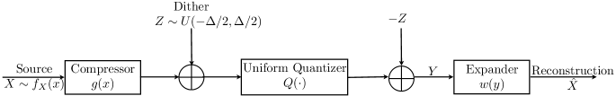
Figure 2: The proposed nonuniform dithered quantizer

II Review of Dithered Quantization

II-A Notation and Preliminaries

In general, lowercase letters (e.g., $x$) denote scalars, boldface lowercase (e.g., $\boldsymbol{x}$) vectors, uppercase (e.g., $U,X$) matrices and random variables, and boldface uppercase (e.g., $\boldsymbol{X}$) random vectors. $\mathbb{E}[\cdot]$, $R_{X}$, and $R_{XZ}$ denote the expectation, covariance of $\boldsymbol{X}$ and cross covariance of $\boldsymbol{X}$ and $\boldsymbol{Z}$ respectively. $\nabla$ denotes the gradient. $\cal N(\boldsymbol{\mu},\boldsymbol{K})$ denotes the Gaussian random vector with mean $\boldsymbol{\mu}$ and covariance matrix $K$.

The entropy of a discrete random vector source $\boldsymbol{X}\in\mathbb{R}^{K}$ taking values in ${\cal X}$ is

$$H(\boldsymbol{X})=-\sum_{\boldsymbol{x}\in{\cal X}}P(\boldsymbol{X}=\boldsymbol{x})\log P(\boldsymbol{X}=\boldsymbol{x})$$ (1)

where logarithm is base 2 to measure it in bits. The differential entropy of a continuous random variable $\boldsymbol{X}$ with probability density function $f_{X}(x)$ is

$$h(\boldsymbol{X})=-\int f_{X}(\boldsymbol{x})\log f_{x}(\boldsymbol{x})d\boldsymbol{x}$$ (2)

The divergence between two densities $f_{X}$ and $g_{X}$, is given by

$$\mathcal{D}(f_{X}||g_{X})=\int f_{X}(\boldsymbol{x})\log\frac{f_{X}(\boldsymbol{x})}{g_{X}(\boldsymbol{x})}d\boldsymbol{x}$$ (3)

The divergence definition above can be extended to conditional densities. For joint densities, $f_{XY}$ and $g_{XY}$ the conditional divergence $\mathcal{D}(f_{X|Y}||g_{X|Y})$ is defined as the divergence between the conditional distributions $f_{X|Y}$ and $g_{X|Y}$ averaged over the density $f_{Y}(\boldsymbol{y})$:

$$\mathcal{D}(f_{X|Y}||g_{X|Y})\!=\!\int\!f_{Y}\!(\boldsymbol{y})\!\int\!f_{X|Y}(\boldsymbol{x,y})\log\frac{f_{X|Y}(\boldsymbol{x,y})}{g_{X|Y}(\boldsymbol{x,y})}d\boldsymbol{x}d\boldsymbol{y}$$ (4)

The mutual information between two random variables $\boldsymbol{X}$ and $\boldsymbol{Y}$ with marginal densities $f_{X}(\boldsymbol{x})$ and $f_{Y}(\boldsymbol{y})$ and a joint density $f_{XY}(\boldsymbol{x},\boldsymbol{y})$ is given by

$${I}(\boldsymbol{X},\boldsymbol{Y})=\int\int f_{X,Y}(\boldsymbol{x},\boldsymbol{y})\log\frac{f_{X,Y}(\boldsymbol{x,y})}{f_{X}(\boldsymbol{x})f_{Y}(\boldsymbol{y})}d\boldsymbol{x}d\boldsymbol{y}$$ (5)

Zero-mean vectors $\boldsymbol{x}\in\mathbb{R}^{K}$ and $\boldsymbol{y}\in\mathbb{R}^{M}$ are said to be uncorrelated if they are orthogonal:

$$\mathbb{E}[\boldsymbol{y}\boldsymbol{x}^{T}]={0}$$ (6)

where the right hand size is $M\times K$ matrix of zeros.

II-B Dithered Quantization

A quantizer is defined by a set of reconstruction points and a partition. The partition $\mathcal{P}=\{\mathcal{P}_{i}\}$ associated with a quantizer is a collection of disjoint regions whose union covers $\mathbb{R}^{K}$. The reconstruction points $\mathcal{R}=\{\boldsymbol{r}_{i}\}$ are typically chosen to minimize a distortion measure. The vector quantizer is a mapping $\mathcal{Q}_{K}:\mathbb{R}^{K}\rightarrow\mathbb{R}^{K}$ that maps every vector $\boldsymbol{X}\in\mathbb{R}^{K}$ into the reconstruction point that is associated with the cell containing $\boldsymbol{X}$, i.e.

$$Q_{K}(\boldsymbol{X})=\boldsymbol{r_{i}}\,\,\,\text{if }\,\,\,\boldsymbol{X}\in\mathcal{P}_{i}$$ (7)

While our theoretical results are general, for a vector quantizer of arbitrary dimensions, for presentation simplicity, we will primarily focus on scalar quantization in the treatment of numerical optimization of nonuniform dithered quantizer and for experimental results. The nonuniform dithered quantization approach is directly extendable to vector quantization by replacing the companded domain uniform quantizer with a lattice quantizer, although at the cost of significantly more challenging numerical optimization.

The scalar uniform quantizer, with reconstructions {$0,\pm\Delta,\pm 2\Delta,...,\pm T\Delta$}, is a mapping $Q:\mathbb{R}\rightarrow\mathbb{R}$ such that

$$Q(x)=i\Delta\,\,\,\text{ for }\,\,i\Delta-\Delta/2<x\leq i\Delta+\Delta/2$$ (8)

In fixed rate quantization, the range parameter $T$ is determined by the rate $R_{f}$

$$R_{f}=\log(2T+1)$$ (9)

while in variable rate quantization $T$ need not, in principle, be finite and we will assume $T\rightarrow\infty$. In this case, uniform quantization is followed by lossless source encoding (entropy coder).

Let dither $Z$ be a random variable, distributed uniformly on the interval $(-\Delta/2,\Delta/2)$. Then, conventional dithered quantizer approximates the source $X$ by

$$\hat{X}=Q(X+Z)-Z$$ (10)

It can be shown that the reconstruction error of this quantizer (denoted $N$) is independent of the source value $X=x$, i.e., $N=\hat{X}-X=Q(X+Z)-Z-X$ is independent of $X$ and uniformly distributed over $(-\Delta/2,\Delta/2)$ for all $X$. Contrast that with a deterministic quantizer, whose error is completely determined by the source value [gershobook].

We note that for this property to hold, the quantizer should span the support of the source density i.e., there should be no overload distortion. While this is often the case for variable rate quantization, for fixed rate overload distortion is inevitable if the source has unbounded support such as a Gaussian source. For practical purposes though, it is common to assume that the source has finite support and we also follow this assumption in our analysis of fixed rate randomized quantization: the quantization error of conventional (uniform) dithered quantization is assumed to be independent of the source.

The realization of the dither random variable $Z$ is available to both the encoder and the decoder. Thus, assuming an optimal entropy coder, the rate of the variable rate quantizer tend to the conditional entropy of the reconstruction given the dither, i.e.,

$$R_{v}=H(\hat{X}|Z)=H(Q(X+Z)|Z)$$ (11)

In [zamiruqr], it was shown that the following holds:

$$H(Q(X+Z)|Z)=h(X+N)-\log\Delta$$ (12)

We will use (12) in the rate calculations of the variable rate (entropy coded) randomized quantization.

III Nonuniform Dithered Quantizer

The main idea is to circumvent the main difficulty due to unequal quantization intervals by performing uniform dithered quantization in the companded domain (see Figure 2). The source $X$ is transformed through compressor $g(\cdot)$ before undergoing dithered uniform quantization. At the decoder side, the dither is subtracted to obtain $Y$. Since we perform uniform dithered quantization in the companded domain, it is easy to show that $Y=g(X)+N$, where $N$ is uniformly distributed over $(-\Delta/2,\Delta/2)$ and independent of the source. The reconstruction is obtained by applying the expander $\hat{X}=w(Y)$. The objective is to find the optimal compressor and expander mappings $g(\cdot),w(\cdot)$ that minimize the expected distortion under the rate constraint. The MSE distortion can be written as:

$$D=\int\int[x-w(g(x)+n)]^{2}f_{X}(x)f_{N}(n)dxdn$$ (13)

where $f_{N}(n)$ is uniform over $(-\Delta/2,\Delta/2)$. Interestingly, this problem bears some similarity to the joint source channel mapping problem where the optimal analog encoding and decoding mappings are studied [emrah_itw10]. In our setting, the quantization error is analogous to the channel noise and the rate constraint in variable rate quantization plays a role similar to that of the power constraint. Similar to [emrah_itw10], we develop an iterative procedure that enforces the necessary conditions for optimality of the mappings. Note that the conventional (uniform) dithered quantizer is a special case employing the trivial identity mappings, i.e., $g(x)\!=\!w(x)\!=\!x,\forall x$.

III-A Optimal Expander

The conditional expectation $w(y)=\mathbb{E}\{X|Y=y\}$ minimizes MSE between the source and the estimate. Hence, the optimal expander $w$ is

$$w(y)=\frac{\int\limits_{\gamma_{-}}^{\gamma_{+}}xf_{X}(x)dx}{\int\limits_{\gamma_{-}}^{\gamma_{+}}f_{X}(x)dx}$$ (14)

where for fixed rate $\gamma_{+}=\min\{g^{-1}(\Delta T),g^{-1}(y+\Delta/2)\}$ and $\gamma_{-}=\max\{g^{-1}(-\Delta T),g^{-1}(y-\Delta/2)\}$, while for variable rate $\gamma_{+}=g^{-1}(y+\Delta/2)$ and $\gamma_{-}=g^{-1}(y-\Delta/2)$.

Note: We restrict the discussion to regular quantizers throughout this paper, hence $g(\cdot)$ is monotonically increasing.

III-B Optimal Compressor

Unlike the expander, the optimal compressor cannot be written in closed form. However, a necessary optimality condition can be obtained by setting the functional derivative of the cost to zero. Thus, a locally optimal compressor $g(\cdot)$, for a given expander $w(\cdot)$, requires that the functional derivative of the total cost, $J$, along the direction of any variation function $\eta(\cdot)$ vanishes [Luenberger], i.e.,

$$\nabla J=\frac{\partial}{\partial\epsilon}\bigg{|}_{\epsilon=0}J\left[{g}({x})+\epsilon{\eta}({x})\right]=0,\,\forall x\in\mathbb{R}$$ (15)

for all admissible perturbation functions $\eta(\cdot)$.

III-B1 Fixed rate

For fixed rate, we have granular distortion, denoted $D_{g}$, and overload distortion, denoted $D_{ol}$. Note that we must account for the overload distortion here, as this constrains $g(x)$ from growing unboundedly in the iterations of the proposed algorithm. Since the rate is fixed, the total cost is identical to the distortion, i.e., $J_{f}=D_{g}+D_{ol}$ where $D_{g}$ and $D_{ol}$ are:

$$D_{g}\!=\!\frac{1}{\Delta}\int\limits_{-\Delta/2}^{\Delta/2}\int\limits_{g^{-1}(-\Delta T)}^{g^{-1}(\Delta T)}[x-w(g(x)+n)]^{2}f_{X}(x)dxdn$$ (16)

$$D_{ol}\! =\frac{1}{\Delta}\int\limits_{-\Delta/2}^{\Delta/2}\left\{\int\limits_{-\infty}^{g^{-1}(-\Delta T)}[x-w(-T\Delta+n)]^{2}f_{X}(x)dx\right.$$

$$\left.+\int\limits_{g^{-1}(\Delta T)}^{\infty}[x-w(T\Delta+n)]^{2}f_{X}(x)dx\right\}dn$$ (17)

III-B2 Variable rate

The rate is obtained via (12) and (12), which require the distribution of $Y=g(X)+N$:

$$f_{Y}(y)=\frac{1}{\Delta}\left[F_{X}(g^{-1}(y+\Delta/2))\!-\!F_{X}(g^{-1}(y-\Delta/2))\right]$$ (18)

where $F_{X}(x)$ is the cumulative distribution function of $X$. The rate is then evaluated as

$$R_{v}=h(Y)-\log\Delta$$ (19)

The total cost for variable rate quantization is $J_{v}=D+\lambda R$ where $\lambda$ is the Lagrangian parameter that is adjusted to obtain the desired rate.

III-C Design Algorithm

The basic idea is to iteratively alternate between enforcing the individual necessary conditions for optimality, thereby successively decreasing the total cost. Iterations are performed until the algorithm reaches a stationary point. Solving for the optimal expander is straightforward since the expander is expressed in closed form as a functional of the known quantities, ${g}({\cdot})$, $f_{X}({\cdot})$. Since the compressor condition is not in closed form, we perform steepest descent, i.e., move in the direction of the functional derivative of the total cost with respect to the compressor mapping $g$. By design, the total cost decreases monotonically as the algorithm proceeds iteratively. The compressor mapping is updated according to (20), where $i$ is the iteration index, $\nabla{J[g(\cdot)]}$ is the directional derivative and $\mu$ is the step size.

$${g}_{i+1}({x})={g}_{i}({x})-\mu\nabla{J[g]}$$ (20)

Note that there is no guarantee that an iterative descent algorithm of this type will converge to the globally optimal solution. The algorithm will converge to a local minimum and hence, initial conditions are important in such greedy optimizations. A low complexity approach to mitigate the poor local minima problem, is to embed within the solution the “noisy channel relaxation” method of [gadkari1999robust, Knagenhjelm]. We initialize the compressor mapping with random initial conditions and run the algorithm for a very low rate (large value for the Lagrangian parameter $\lambda$). Then, we gradually increase the rate (decrease $\lambda$) while tracking the minimum. Note that local minima problem is more pronounced at multi-dimensional optimizations, which hence requires more powerful non-convex optimization tools such as deterministic annealing [da]. In our design and experiments, we focus on scalar compressor and expander and we did not observe significant local minima problems.

IV Reconstruction Error Uncorrelated with the Source

In this section, we propose two quantization schemes (one deterministic, one randomized) that satisfy the constraint that reconstruction error be uncorrelated with the source.

IV-A Constrained Deterministic Quantizer

A deterministic quantizer cannot yield quantization noise independent of the source [gershobook]. However, it is possible to render the quantization noise uncorrelated with the source. An early prior work along this line appeared in [oba], where a uniform quantizer is converted to a quantizer whose quantization noise is uncorrelated with the source, by adjusting the reconstruction points. In this section, we derive the optimal (nonuniform in general) deterministic quantizer which is constrained to give quantization error uncorrelated with the source.

Let $\boldsymbol{r}_{i}$ and ${\widehat{\boldsymbol{r_{i}}}}$ be the reconstruction points and $\mathcal{P}_{i}$ and ${\widehat{\mathcal{P}_{i}}}$ represent the $i^{th}$ quantization region, for the constrained (i.e., whose quantization error is uncorrelated with the source) and unconstrained MSE optimal quantizer, respectively. Also, let $p_{i}$ and $\widehat{p}_{i}$ denote the probability of $\boldsymbol{X}$ falling into the $i^{th}$ cell of these respective quantizers.

Theorem 1.

$\mathcal{P}_{i}={\widehat{\mathcal{P}_{i}}}\,\,\,\text{and}\,\,\,\boldsymbol{r_{i}}=\boldsymbol{C}{\boldsymbol{\hat{r}_{i}}},\forall i$ where

$$\boldsymbol{C}={R}_{X}\left(\sum\limits_{i=1}^{M}p_{i}{\boldsymbol{\hat{r}_{i}}}{\boldsymbol{\hat{r}_{i}^{T}}}\right)^{-1}.$$

Proof.

We start with the fixed rate analysis. Let $M$ denote the number of quantization cells. The distortion can be expressed as

$$D=\sum\limits_{i=1}^{M}\int\limits_{\boldsymbol{x}\in\mathcal{P}_{i}}{(\boldsymbol{x}-\boldsymbol{r}_{i})^{T}(\boldsymbol{x}-\boldsymbol{r}_{i})f_{X}(\boldsymbol{x})\,d\boldsymbol{x}}$$ (21)

and the “uncorrelatedness” constraint may be stated via the orthogonality principle

$$\sum\limits_{i=1}^{M}\int\limits_{\boldsymbol{x}\in\mathcal{P}_{i}}\boldsymbol{x}(\boldsymbol{x}-\boldsymbol{r}_{i})^{T}f_{X}(\boldsymbol{x})\,d\boldsymbol{x}=\boldsymbol{0}$$ (22)

Note further that (22) can be written as:

$$\sum\limits_{i=1}^{M}\boldsymbol{r}_{i}\boldsymbol{l}_{i}^{T}={R}_{X}\text{ where }\boldsymbol{l}_{i}=\int\limits_{\boldsymbol{x}\in\mathcal{P}_{i}}\boldsymbol{x}f_{X}(\boldsymbol{x})\,d\boldsymbol{x}$$ (23)

The constrained problem of minimizing $D$ subject to $\sum\limits_{i=1}^{M}\boldsymbol{r}_{i}\boldsymbol{l}_{i}^{T}={R}_{X}$ is equivalent to the unconstrained minimization of Lagrangian $J$:

$$J=D+\sum\limits_{k=1}^{K}\boldsymbol{\gamma}(k)^{T}\left[{R}_{X}(k)-\sum\limits_{i=1}^{M}\boldsymbol{r}_{i}\boldsymbol{l}_{i}(k)\right]$$ (24)

where $\boldsymbol{\gamma}=[\boldsymbol{\gamma}(1)\,\,\,\boldsymbol{\gamma}(2)...\,,\boldsymbol{\gamma}(K)]$ denotes the $K\times K$ multiplier Lagrangian matrix, ${R}_{X}(k)$ denotes the $k^{th}$ column of ${R}_{X}$ and $l_{i}(k)$ denotes the $k^{th}$ element of $\boldsymbol{l}_{i}$. By setting $\nabla_{r_{i}}J=\boldsymbol{0}$, we obtain the condition:

$$\nabla_{r_{i}}J=-2\boldsymbol{l}_{i}^{T}+2p_{i}\boldsymbol{r}_{i}^{T}-\sum\limits_{k=1}^{K}\gamma(k)^{T}{l}_{i}(k)=\boldsymbol{0}$$ (25)

Noting that $\sum_{k=1}^{K}\gamma(k)^{T}{l}_{i}(k)=\boldsymbol{l}_{i}^{T}\boldsymbol{\gamma}$,we obtain $\boldsymbol{r}_{i}=\frac{1}{p_{i}}{C}\boldsymbol{l}_{i}$ where ${C}$ is a constant $M\times M$ matrix. $\boldsymbol{C}$ is found by plugging this into (23):

$$\boldsymbol{C}={R}_{X}\left(\sum\limits_{i=1}^{M}\frac{1}{p_{i}}\boldsymbol{l}_{i}\boldsymbol{l}_{i}^{T}\right)^{-1}$$ (26)

Note that $\boldsymbol{l}_{i}/p_{i}$ is the MSE optimal reconstruction of an unconstrained quantizer that shares the same decision boundary with the constrained one, $\mathcal{P}_{i}$. Plugging (26) into (21) and after some algebraic manipulations, we obtain:

$$D=\frac{\sigma_{X}^{2}}{\sigma_{X}^{2}-D^{*}}D^{*}$$ (27)

where $D^{*}$ is the distortion associated with the quantizer given by $\mathcal{P}_{i}$ and with corresponding optimal reconstruction points $\boldsymbol{l}_{i}/p_{i}$. (27) implies that $D$ achieves its minimum whenever $D^{*}$ is minimized. Hence,

$$\mathcal{P}_{i}=\widehat{\mathcal{P}_{i}}\Rightarrow\boldsymbol{l}_{i}=p_{i}\boldsymbol{\hat{r_{i}}}$$ (28)

Plugging (28) into (26), we obtain the result. The proof for variable rate follows similar lines, with the only modification that we now have to account for the rate term $R=\sum\limits_{i=1}^{M}p_{i}\log p_{i}$. The uncorrelatedness constraint is identical to the one in fixed rate, hence the overall Lagrangian cost can be expressed as:

$$J=D+\sum\limits_{k=1}^{M}\boldsymbol{\gamma}(k)^{T}\left[\boldsymbol{R}_{X}(k)-\sum\limits_{i=1}^{M}\boldsymbol{r}_{i}\boldsymbol{l}_{i}(k)\right]+\lambda\sum\limits_{i=1}^{M}p_{i}\log p_{i}$$ (29)

By setting $\nabla_{r_{i}}J=\boldsymbol{0}$ and following the same steps, we obtain:

$$\boldsymbol{r}_{i}=\frac{1}{p_{i}}\boldsymbol{R}_{X}\left(\sum\limits_{i=1}^{M}\frac{1}{p_{i}}\boldsymbol{l}_{i}\boldsymbol{l}_{i}^{T}\right)^{-1}\boldsymbol{l}_{i}$$ (30)

Note that (27) holds due to (30) and the optimal unconstrained quantizer achieves the minimum distortion $D^{*}$ subject to the rate constraint. This indicates that the constrained and unconstrained quantizers have identical $p_{i}$ and hence $\mathcal{P}_{i}=\widehat{\mathcal{P}_{i}}$ which implies $\boldsymbol{l}_{i}=p_{i}\boldsymbol{\hat{r_{i}}}$. Plugging $\boldsymbol{l}_{i}=p_{i}\boldsymbol{\hat{r_{i}}}$ into (30), we obtain the desired result.

■

IV-B Constrained Randomized Quantizer

Due to the effect of companding, the nonuniform randomized quantizer we derived in Section III does not guarantee reconstruction error uncorrelated with the source even though it builds on the (conventional) dithered quantizer whose quantization error is independent of the source. We therefore explicitly constrain the randomized quantizer to generate uncorrelated reconstruction error, by adding a penalty term to the total cost function. The Lagrangian parameter $\lambda_{c}\geq 0$ is set to ensure $\mathbb{E}\{xw(g(x)+n)\}=\mathbb{E}\{x^{2}\}$.

$$J_{c}=J+\lambda_{c}\mathbb{E}[x^{2}-xw(g(x)+n)]$$ (31)

where $J=J_{v}$ in the case of variable rate and $J=J_{f}$ for fixed rate. We find the necessary conditions of optimality of constrained compressor and expander mappings at fixed and variable rate, by setting the functional derivative of the total cost ($J_{c}$) to zero. Surprisingly, the optimally constrained compressor mapping remains unchanged (compared to the unconstrained optimal compressor) and the only modification of the optimally constrained expander mapping is simple scaling. We state this result in the following theorem.

Theorem 2.

Let $g$ and $w$ be the compressor and expander mappings of the unconstrained optimal randomized quantizer. Let $g_{c}$ and $w_{c}$ denote the optimal mappings subject to the constraint that the reconstruction error be uncorrelated with the source. Then,

$$g_{c}(x)=g(x),w_{c}(y)=(1-\lambda_{c})w(y)$$ (32)

where $\lambda_{c}$ is the Lagrangian multiplier of (31).

Note that this result applies to both fixed and variable rate.

Proof.

The optimal expander is no longer the standard conditional expectation, since it is impacted by the constraint. By setting

$$\frac{\partial}{\partial\epsilon}\bigg{|}_{\epsilon=0}J_{c}\left[{w}({y})+\epsilon{\eta}({y})\right]=0$$ (33)

we obtain the optimal expander in closed form as $w_{c}(y)=(1-\lambda_{c})w(y)$. The update rule for $g_{c}(x)$ can be derived similarly. Setting

$$\frac{\partial}{\partial\epsilon}\bigg{|}_{\epsilon=0}J_{c}\left[{g}({x})+\epsilon{\eta}({x})\right]=0$$ (34)

and plugging $w_{c}(y)=(1-\lambda_{c})w(y)$ yields, after straightforward algebra, $g_{c}(x)=g(x)$. ■

V Asymptotic Analysis

V-A Rate-Distortion Functions

To quantify theoretically how much a source can be compressed under the independent/uncorrelated reconstruction error constraint, we define two rate-distortion functions in which we respectively constrain the reconstructions error to be i) uncorrelated with the source $R_{U}(D)$, and ii) independent of the source $R_{I}(D)$.

Assume that we have source $X$ with density $f_{X}(\cdot)$ that produces the independent identically distributed (i.i.d.) sequence $X_{1},X_{2},..,X_{n}$ denoted as $X^{n}$. Similarly, let ${\hat{X}_{1}},{\hat{X}_{2}},..,{\hat{X}_{n}}$ be the reconstruction sequence, denoted as ${\hat{X}^{n}}$. Let $S^{n}=X^{n}-{\hat{X}^{n}}$ be the i.i.d. sequence of reconstruction errors with marginal density $f_{S}(\cdot)$. Let $f_{XS}(x,s)$ denote joint distribution of $X$ and $S$ and $d(X^{n},\hat{X}^{n})$ denote the distortion measure between sequences $X^{n}$ and $\hat{X}^{n}$ defined as

$$d(X^{n},\hat{X}^{n})=\frac{1}{n}\sum\limits_{i=1}^{n}d(X_{i},\hat{X}_{i})$$ (35)

Let us recall the classical rate-distortion result in information theory:

Rate-distortion Theorem: (eg. [coverbook]).

Let $R(D)$ be the infimum of all achievable rates $R$ with average distortion $\mathbb{E}[d(X^{n},X^{n}+S^{n})]\leq D$ as $n\rightarrow\infty$. Then,

$$R(D)=\inf_{\begin{subarray}{c}S:\mathbb{E}[d(X,X+S)]\leq{D}\end{subarray}}I(X;X+S)$$ (36)

We next focus on our problem: let $R_{U}(D)$ be the infimum of all achievable rates $R$ with average distortion

$$\lim_{n\rightarrow\infty}\mathbb{E}[d(X^{n},X^{n}+S^{n})]\leq D$$ (37)

subject to the constraint

$$\mathbb{E}[X_{i}S_{i}]=0,i=1,2,..,n$$ (38)

as ${n\to\infty}$. Similarly, let $R_{I}(D)$ be the infimum of all achievable rates $R$ with average distortion $\mathbb{E}[d(X^{n},X^{n}+S^{n})]\leq D$ subject to the constraint $S_{i}$ is independent of $X_{i}$ for all $i$, as ${n\to\infty}$. Then, we have the following result characterizing the fundamental limits of source compression under the constraints that reconstruction error is uncorrelated with or independent of the source.

Theorem 3.

$$R_{U}(D)=\inf_{\begin{subarray}{c}S:\mathbb{E}[d(X,X+S)]\leq{D}\\ \mathbb{E}[XS]=0\end{subarray}}I(X;X+S)$$ (39)

$$R_{I}(D)=\inf_{\begin{subarray}{c}S:{\mathbb{E}[d(X,X+S)]}\leq{D}\\ \mathcal{D}(f_{XS}(X,S)||f_{X}(X)f_{S}(S))=0\end{subarray}}I(X;X+S)$$ (40)

Proof.

Consider the distortion measures

$$d_{U}(x,x+s)=d(x,x+s)+\beta||xs||$$ (41)

$$d_{I}(x,x+s)=d(x,x+s)+\beta\log\frac{f_{XS}(x,s)}{f_{X}(x)f_{S}(s)}$$ (42)

for some $\beta>0$.

We next consider the rate-distortion functions (denoted $R_{U}^{*}(D)$ and $R_{I}^{*}(D)$) associated with these distortion measures. By replacing $d$ with $d_{U}$ and $d_{I}$ in the standard rate-distortion functions, we obtain the following expressions:

$$R_{U}^{*}(D)=\inf_{\begin{subarray}{c}S:\mathbb{E}[d_{U}(X,X+S)]\leq D\end{subarray}}I(X;X+S)$$ (43)

$$R_{I}^{*}(D)=\inf_{\begin{subarray}{c}S:\mathbb{E}[d_{I}(X,X+S)]\leq D\end{subarray}}I(X;X+S)$$ (44)

We note that the achievability and the converse proofs are straightforward extensions of the standard achievability and the converse proofs for regular rate distortion function.

We next consider the distortion measures $d_{U}$ and $d_{I}$ and associated rate-distortion functions $R_{U}^{*}(D)$ and $R_{I}^{*}(D)$ when $\beta\rightarrow\infty$. As $\beta\rightarrow\infty$, $\mathbb{E}[d_{U}(X^{n},X^{n}+S^{n})]\leq D$ implies $\mathbb{E}[d(X^{n},X^{n}+S^{n})]\leq D$ while $\mathbb{E}[X_{i}S_{i}]\rightarrow 0$ for all $i$. Similarly, as $\beta\rightarrow\infty$, $\mathbb{E}[d_{I}(X^{n},X^{n}+S^{n})]\leq D$ implies $\mathbb{E}[d(X^{n},X^{n}+S^{n})]\leq D$ under the constraint that $X_{i}$ and $S_{i}$ are asymptotically independent for all $i$. Hence, as $\beta\rightarrow\infty$, the distortion measures under consideration satisfy the respective requirements of uncorrelatedness or independence, i.e., $R_{U}(D)=R_{U}^{*}(D)$ and $R_{I}(D)=R_{I}^{*}(D)$.

Hence, (39) and (40) are indeed the information theoretical characterization of the limits of encoding a source with uncorrelated and independent reconstruction error respectively. ■

V-B Gaussian Vector Source with MSE Distortion

In this section, we examine a special case where the source is vector Gaussian and the distortion measure is squared error. We start with an auxiliary lemma without proof (see eg. [coverbook] for the proof).

Lemma 1 ([coverbook]).

Let $\boldsymbol{S}\sim f_{S}$ and $\boldsymbol{S}_{G}\sim f_{S_{G}}$ be random vectors in $\mathbb{R}^{K}$with the same covariance matrix ${R}_{S}$. If $\boldsymbol{S}_{G}\sim\mathcal{N}(\boldsymbol{0},{R}_{S})$ then

$$\mathbb{E}_{S_{G}}[\log(f_{S_{G}}(\boldsymbol{S}))]=\mathbb{E}_{S}[\log(f_{S_{G}}(\boldsymbol{S}))]$$ (45)

where $\mathbb{E}_{S_{G}}$ and $\mathbb{E}_{S}$ denote the expectations with respect to $f_{S_{G}}$ and $f_{S}$ respectively.

Let us present a key lemma regarding the mutual information of two correlated random vectors constrained to have a fixed cross covariance matrix.

Lemma 2.

Let $\boldsymbol{X}\sim\mathcal{N}(\boldsymbol{0},{R}_{X})$ and $\boldsymbol{S}_{G}\sim\mathcal{N}(\boldsymbol{0},{R}_{S})$ be jointly Gaussian random vectors in $\mathbb{R}^{K}$. Let $\boldsymbol{S}\in\mathbb{R}^{K}$ and $\boldsymbol{S}_{G}$ have the same covariance matrix, ${R}_{S}$ and the same cross covariance matrix with $\boldsymbol{X}$, ${R}_{SX}$. Then,

$$I(\boldsymbol{X},\boldsymbol{X}+\boldsymbol{S})\geq I(\boldsymbol{X},\boldsymbol{X}+\boldsymbol{S}_{G})$$ (46)

with equality if and only if $\boldsymbol{S}\sim\mathcal{N}(\boldsymbol{0},{R}_{S})$.

Proof.

Consider $\gamma\!=\!I(\boldsymbol{X},\boldsymbol{X}\!+\!\boldsymbol{S})\!-\!I(\boldsymbol{X},\boldsymbol{X}\!+\!\boldsymbol{S}_{G})$. Plugging the expressions, we obtain:

$$\gamma=h(\boldsymbol{X}|\boldsymbol{S_{G}}+\boldsymbol{X})-h(\boldsymbol{X}|\boldsymbol{S}+\boldsymbol{X})$$ (47)

Noting that $h(\boldsymbol{X}|\boldsymbol{S_{G}}+\boldsymbol{X})=h(\boldsymbol{S_{G}}|\boldsymbol{S_{G}}+\boldsymbol{X})$ and $h(\boldsymbol{X}|\boldsymbol{S}+\boldsymbol{X})=h(\boldsymbol{S}|\boldsymbol{S}+\boldsymbol{X})$ and plugging $\boldsymbol{Y}=\boldsymbol{X}+\boldsymbol{S}$ and $\boldsymbol{Y}_{G}=\boldsymbol{X}+\boldsymbol{S}_{G}$, we obtain:

$$\gamma=h(\boldsymbol{S}_{G}|\boldsymbol{Y}_{G})-h(\boldsymbol{S}|\boldsymbol{Y})=$$ (48)

$$\!\!\!\int\!\!\!\int\!\!\!\left\{f_{S,Y}(\boldsymbol{s},\!\boldsymbol{y})\!\log f_{S|Y}(\boldsymbol{s},\boldsymbol{y})\!\!\!-\!\!\!f_{S_{G},Y_{G}}(\boldsymbol{s},\!\boldsymbol{y})\!\log f_{S_{G}|Y_{G}}\!(\boldsymbol{s},\boldsymbol{y})\!\right\}\!d\boldsymbol{s}d\boldsymbol{y}\!\!\!$$ (49)

Using Lemma 1 and the fact that the joint distribution $f_{S_{G},Y_{G}}$ is Gaussian:

$$= \!\!\!\int\!\!\!\int\!\!\!f_{S,Y}(\boldsymbol{s},\boldsymbol{y})\left[\log f_{S|Y}(\boldsymbol{s},\boldsymbol{y})\!-\!\log f_{S_{G}|Y_{G}}(\boldsymbol{s},\boldsymbol{y})\right]d\boldsymbol{s}d\boldsymbol{y}$$ (50)

$$= \int f_{Y}(\boldsymbol{y})\int f_{S|Y}(\boldsymbol{s},\boldsymbol{y})\log\frac{f_{S|Y}(\boldsymbol{s},\boldsymbol{y})}{f_{S_{G}|Y_{G}}(\boldsymbol{s},\boldsymbol{y})}d\boldsymbol{s}d\boldsymbol{y}$$ (51)

$$= \mathcal{D}(f_{S|Y},f_{S_{G}|Y_{G}})$$ (52)

$\mathcal{D}\geq 0$ with equality if and only if $\boldsymbol{S}\sim\mathcal{N}(\boldsymbol{0},{R}_{S}).$

■

Next,wepresentourmainresultonthistopic:

Theorem 4.

ForaGaussianvectorsourceX∈RKan