Implications of gauge-mediated supersymmetry breaking with vector-like quarks and a $\sim$125 GeV Higgs boson

Abstract

We investigate the implications of models that achieve a Standard Model-like Higgs boson of mass near 125 GeV by introducing additional TeV-scale supermultiplets in the vector-like ${\bf 10}+\overline{\bf 10}$ representation of $SU(5)$, within the context of gauge-mediated supersymmetry breaking. We study the resulting mass spectrum of superpartners, comparing and contrasting to the usual gauge-mediated and CMSSM scenarios, and discuss implications for LHC supersymmetry searches. This approach implies that exotic vector-like fermions $t^{\prime}_{1,2}$, $b^{\prime}$,and $\tau^{\prime}$ should be within the reach of the LHC. We discuss the masses, the couplings to electroweak bosons, and the decay branching ratios of the exotic fermions, with and without various unification assumptions for the mass and mixing parameters. We comment on LHC prospects for discovery of the exotic fermion states, both for decays that are prompt and non-prompt on detector-crossing time scales.

I Introduction

Recently the ATLAS and CMS experiments at the LHC have put forward data analysis results that suggest the Higgs boson mass could be close to $125\,{\rm GeV}$ ATLAScombined ; CMScombined . The statistical significance is not at the ‘discovery level’, nor is it enough to determine if the putative Higgs boson signal is really that of the Standard Model (SM) Higgs boson, or some close cousin that may have somewhat different couplings and rates. Nevertheless, we wish to investigate the supposition that the Higgs boson exists at this mass and is SM-like in its couplings.

Stipulating the above, supersymmetry is an ideal theoretical framework to accommodate the results. The many favorable features of supersymmetry are well-known primer , but the one most applicable here is its generic prediction for a SM-like Higgs boson with mass less than about $130\,{\rm GeV}$. Within some frameworks of supersymmetry, such as ‘natural’ versions of minimal supergravity (mSUGRA) or minimal gauge mediated supersymmetry breaking (GMSB), a Higgs mass value of $\sim\!\!125\,{\rm GeV}$ seems perhaps uncomfortably high. Within other frameworks, such as ‘unnatural’ PeV-scale supersymmetry PeVSUSY or split supersymmetry splitSUSY , such a mass value seems perhaps uncomfortably low. Nevertheless, almost any approach to supersymmetry allows one to easily absorb this Higgs mass into the list of defining data and then present the resulting allowed parameter space.

In this article we wish to see how well one can explain a $\sim\!\!125\,{\rm GeV}$ Higgs boson mass using ‘natural’ supersymmetry. There are many good discussions of this already present in the literature lightstopscenario ; otherscenarios , but the approach we take here is to use extra vector-like matter supermultiplets to raise the Higgs mass Moroi:1991mg -Nakayama:2012zc . As shown in detail in Martin:2009bg , the Yukawa coupling of the vector-like quarks to the Higgs has a fixed point at a value large enough to substantially increase the lightest Higgs mass while giving a fit to precision electroweak oblique observables that is as good as, or slightly better than, the SM. This can be done in various different scenarios for the soft terms, but here we choose to investigate within the context of GMSB; earlier studies of this can be found in Endo:2011mc ; Evans:2011uq ; Endo:2011xq ; Endo:2012rd ; Nakayama:2012zc . The details of the specific model we study will be discussed in the next section. We like this approach because the superpartner masses are not required to become extremely heavy to raise the light Higgs mass through large logarithms in the radiative corrections, nor does one need to invoke very large Higgs-stop-antistop supersymmetry-breaking couplings. Instead, the extra vector-like states, interacting with the Higgs boson, make extra contributions to the Higgs boson mass in a natural way. This approach has been reemphasized recently also by Li:2011ab -Nakayama:2012zc within the context of the $\sim\!\!125\,{\rm GeV}$ Higgs boson signal, and our study confirms some previous results and extends the understanding by investigating correlations within a unified theory and detailing the phenomenological implications that can be useful for the LHC experiments to confirm or reject this hypothesized explanation for the Higgs boson mass value.

II Minimal GMSB model with extra vector-like particles

II.1 Theory definition, parameters and spectrum

The theory under consideration here is a minimal GMSB theory with one $SU(5)$ ${\bf 5}+\overline{\bf 5}$ messenger multiplet pair, along with a ${\bf 10}+\overline{\bf 10}$ multiplet pair at the TeV scale. We choose this model because it is minimal, illustrates the key phenomenological features of this broad class of theories, and maintains perturbative gauge coupling unification at the high scale. The same model has also been considered in Endo:2011mc ; Evans:2011uq ; Endo:2011xq ; Endo:2012rd ; Nakayama:2012zc . The unification scale (defined as the scale where $g_{1}$ and $g_{2}$ meet) turns out to be larger than the corresponding scale in the MSSM by a factor of 2-4, depending on the sparticle thresholds and the GMSB messenger scale. As in ref. Martin:2009bg , we use 3-loop beta functions for the gauge couplings and gaugino masses, and 2-loop beta functions for all other parameters. These renormalization group equations are not given explicitly here, because they can be obtained in a straightforward and automated way from the general results given in refs. betas:1 ; betas:2 ; betas:3 .

To set the notation, the MSSM fields are defined below along with their $SU(3)_{C}\times SU(2)_{L}\times U(1)_{Y}$ quantum numbers:

$$q_{i}=({\bf 3},{\bf 2},1/6),~{}~{}~{}~{}\overline{u}_{i}=({\bf\overline{3}},{\bf 1},-2/3),~{}~{}~{}~{}\overline{d}_{i}=({\bf\overline{3}},{\bf 1},1/3),~{}~{}~{}~{}$$

$$\ell_{i}=({\bf 1},{\bf 2},-1/2),~{}~{}~{}~{}\overline{e}_{i}=({\bf 1},{\bf 1},1),~{}~{}~{}~{}H_{u}=({\bf 1},{\bf 2},1/2),~{}~{}~{}~{}H_{d}=({\bf 1},{\bf 2},-1/2).$$ (2.1)

with $i=1,2,3$ denoting the three families. The MSSM superpotential, in the approximation that only third-family Yukawa couplings are included, is

$$W_{\rm MSSM}=\mu H_{u}H_{d}+y_{t}H_{u}q_{3}\overline{u}_{3}-y_{b}H_{d}q_{3}\overline{d}_{3}-y_{\tau}H_{d}\ell_{3}\overline{e}_{3}.$$ (2.2)

The ${\bf 10}$ and $\overline{\bf 10}$ $SU(5)$ multiplets are comprised of $Q$, $\overline{U}$, $\overline{E}$ and $\overline{Q}$, $U$, $E$ supermultiplets, respectively, with

$$Q=({\bf 3},{\bf 2},1/6),~{}~{}~{}~{}~{}~{}U=({\bf 3},{\bf 1},2/3),~{}~{}~{}~{}~{}~{}E=({\bf 1},{\bf 1},-1),$$ (2.3)

$$\overline{Q}=(\overline{\bf 3},{\bf 2},-1/6),~{}~{}~{}~{}~{}~{}\overline{U}=(\overline{\bf 3},{\bf 1},-2/3),~{}~{}~{}~{}~{}~{}\overline{E}=({\bf 1},{\bf 1},1).$$ (2.4)

These extra fields interact with the MSSM Higgs bosons at the renormalizable level. The relevant superpotential is

$$W_{QUE}=M_{Q}Q\overline{Q}+M_{U}U\overline{U}+M_{E}E\overline{E}+kH_{u}Q\overline{U}-k^{\prime}H_{d}\overline{Q}U.$$ (2.5)

The extra superfields of the ${\bf 10}+\overline{\bf 10}$ give rise to additional exotic particles beyond the MSSM: charge $+2/3$ quarks $t^{\prime}_{1,2}$ (plus scalar superpartners $\tilde{t}^{\prime}_{1,2,3,4}$), a charge $-1/3$ quark $b^{\prime}$ (plus scalar superpartners $\tilde{b}^{\prime}_{1,2}$), and a charged lepton $\tau^{\prime}$ (plus scalar superpartners $\tilde{\tau}^{\prime}_{1,2}$).

As noted in Martin:2009bg , the Yukawa interaction $k$ is subject to an infrared-stable quasi-fixed point Hill:1980sq slightly above $k=1.0$ at the TeV scale. This value is both natural (since a large range of high-scale input values closely approaches it), and is easily large enough to mediate a correction to the lightest Higgs boson mass $M_{h}$ that can accommodate $M_{h}\sim\!\!125\,{\rm GeV}$ or larger, depending of course on the other parameters of the theory. In this paper, we will always assume that $k$ is near its (strongly attractive) quasi-fixed point, by arbitrarily taking $k=1$ near the apparent scale of gauge coupling unification and evolving it down. Taking larger values at the high scale would only increase the TeV-scale value of $k$ by about 2% at most, although it should be kept in mind that the contribution to the Higgs squared mass correction scales like $k^{4}$. For simplicity, we will take $k^{\prime}$ to be small, since it does not help to raise the $h^{0}$ mass, although a small non-zero value would not affect the results below very much. The superpartner spectrum of this theory is determined by the normal procedures for minimal GMSB. The input parameters needed are $\tan\beta$, ${\rm sign}(\mu)$, the mass scale for the $\bf{5}+\overline{\bf 5}$ messenger masses ${M_{\rm mess}}$ and the supersymmetry breaking transmission scale $\Lambda$ which is equal to $\langle F_{S}\rangle/\langle S\rangle$ where $\langle F_{S}\rangle$ and $\langle S\rangle$ are vacuum expectation values of the $F$-component and scalar component of the chiral superfield $S$ that couples directly to the messenger sector. Using standard techniques primer one can then compute the superpartner spectrum and Higgs boson mass spectrum. Corrections to the lightest Higgs boson mass $M_{h}$ are obtained using the full one-loop effective potential approximation, as in Martin:2009bg . (We have checked the MSSM contributions against FeynHiggs FeynHiggs and we find agreement to within expected uncertainties of 1-2 GeV.) One-loop corrections to the pole masses of all strongly interacting particles are also included; these are particularly important for the gluino.

If the exotic states only interacted among themselves and the Higgs fields, then a $Z_{2}$ quantum number could be defined on the superpotential with odd assignments to $Q,\overline{Q},U,\overline{U},E,\overline{E}$ and even assignments for everything else, leading to stability of the lightest new fermion state. At the renormalizable level, the only way the lightest new quark $t_{1}^{\prime}$ and the $\tau^{\prime}$ can decay is by breaking this $Z_{2}$ symmetry via superpotential mixing interactions with MSSM states,

$$W_{\rm mix}=\epsilon_{\scriptscriptstyle U}H_{u}q_{3}\overline{U}+\epsilon^{\prime}_{\scriptscriptstyle U}H_{u}Q\overline{u}_{3}-\epsilon_{\scriptscriptstyle D}H_{d}Q\overline{d}_{3}-\epsilon_{\scriptscriptstyle E}H_{d}\ell_{3}\overline{E},$$ (2.6)

where $\epsilon_{\scriptscriptstyle U}$, $\epsilon^{\prime}_{\scriptscriptstyle U}$, $\epsilon_{\scriptscriptstyle D}$, and $\epsilon_{\scriptscriptstyle E}$ are new Yukawa couplings. Note that this is consistent with matter parity provided that the supermultiplets $Q,\overline{Q},U,\overline{U},E,\overline{E}$ are assigned odd matter parity, so that the new fermions have even $R$-parity. We assume that the mixing Yukawa couplings are confined to the third-family MSSM fields $q_{3},\overline{u}_{3},\overline{d}_{3},\ell_{3}$, in order to avoid dangerous flavor violating effects; the bounds on third-family mixings with new heavy states are much less stringent than for first and second-family quarks and leptons fourthflavor ; KPST . As we will see in section IV, couplings less than $0.1$ to third generation quarks and leptons are easily small enough to avoid all flavor constraints. Assuming this for simplicity, then $\epsilon_{\scriptscriptstyle U}$, $\epsilon^{\prime}_{\scriptscriptstyle U}$, $\epsilon_{\scriptscriptstyle D}$, and $\epsilon_{\scriptscriptstyle E}$ are small enough to be neglected in wave function renormalizations, and so do not contribute to other couplings’ renormalization group equations, and only contribute linearly to their own. Furthermore, their effects on the mass eigenstates of the new particles can be treated as small perturbations.

It is interesting to consider the case of $SU(5)$-symmetric interactions near the unification scale. If one assigns $H_{u}$ and $H_{d}$ to the ${\bf 5}$ and ${\bf\overline{5}}$ representations respectively, and $Q,\overline{U},\overline{E}$ to the ${\bf 10}$ and $\overline{Q},U,E$ to the ${\bf\overline{10}}$, then one has

$$M_{Q}=M_{U}=M_{E},$$ (2.7)

$$\epsilon_{\scriptscriptstyle U}=\epsilon^{\prime}_{\scriptscriptstyle U},\qquad\quad\epsilon_{\scriptscriptstyle D}=\epsilon_{\scriptscriptstyle E}.$$ (2.8)

at the unification scale. The further unification in $SO(10)$ implies the stronger condition

$$\epsilon_{\scriptscriptstyle U}=\epsilon^{\prime}_{\scriptscriptstyle U}=\epsilon_{\scriptscriptstyle D}=\epsilon_{\scriptscriptstyle E}.$$ (2.9)

A logical guess is that the origin of the masses $M_{Q},M_{U},M_{E}$ is similar to that of the MSSM $\mu$ term, and might occur well below the unification scale. For example, one can imagine that they arise from non-renormalizable superpotential operators like

$$W=\frac{1}{M_{P}}S\overline{S}(\lambda_{\mu}H_{u}H_{d}+\lambda_{Q}Q\overline{Q}+\lambda_{U}U\overline{U}+\lambda_{E}E\overline{E}),$$ (2.10)

where $S$, $\overline{S}$ are SM singlet fields (possibly the same) which carry a Peccei-Quinn charge and get vacuum expectation values (VEVs) at an intermediate scale, as recently proposed in this context by Nakayama:2012zc , giving rise to masses $\mu=\lambda_{\mu}\langle S\overline{S}\rangle/M_{P}$ and $M_{Q,U,E}=\lambda_{Q,U,E}\langle S\overline{S}\rangle/M_{P}$. Note that if the dimensionless couplings $\lambda_{Q,U,E}$ are small, then their renormalization group evolution from the apparent unification scale down to the scale at which $S,\overline{S}$ get VEVs is the same as that of the corresponding masses $M_{Q,U,E}$, depending only on the wavefunction renormalization anomalous dimensions of the chiral superfields $Q,\overline{Q},U,\overline{U},E,\overline{E}$. In this case, it is sensible to evolve the masses as if they were the same at the scale of apparent gauge coupling unification, based on an assumed unification of the corresponding superpotential couplings $\lambda_{Q,U,E}$. Of course, the relations (2.7) and (2.9) are certainly not mandatory. The tree-level relations between couplings (or masses) implied by GUT groups can be greatly modified by non-renormalizable terms, alternative assignments of the Higgs fields, and mixing effects near the GUT scale. However, eqs. (2.7) and (2.9) do constitute a plausible and useful benchmark case that we will use for some of the explorations in this paper. At the TeV scale, typical values obtained from the renormalization group running are then:

$$M_{Q}:M_{U}:M_{E} \approx 1.8:1:0.45,$$ (2.11)

with some variation at the $<$20% level due to the choice of GMSB messenger scale and $\Lambda$. (The ratios $M_{Q}/M_{U}$ and $M_{U}/M_{E}$ at the TeV scale tend to decrease with larger $M_{\rm mess}$ and $\Lambda$.) The ratios of mixing couplings also exhibit a pattern when the unification condition eq. (2.9) is assumed, but with a strong dependence on the trajectory for $k$. In general one finds $\epsilon^{\prime}_{\scriptscriptstyle U}$ slightly larger than $\epsilon_{\scriptscriptstyle U}$, and $\epsilon_{\scriptscriptstyle D}$ larger than $\epsilon_{\scriptscriptstyle U}$ by a factor of 3.5 to 6. In the following, we will sometimes consider the typical case

$$\epsilon_{\scriptscriptstyle U}:\epsilon^{\prime}_{\scriptscriptstyle U}:\epsilon_{\scriptscriptstyle D} \approx 1:1.15:4.5$$ (2.12)

as a benchmark for illustration when considering the branching ratios of $t_{1}^{\prime}$ and $b^{\prime}$.

The model we study here is not the unique extension of GMSB models to include vector-like quarks that raise the Higgs mass. One can replace the $U+\overline{U}$ fields by $D+\overline{D}+E+\overline{E}$ fields without changing the prospects for perturbative gauge coupling unification, as discussed in Martin:2009bg . In that case, a Yukawa coupling $H_{u}\overline{Q}D$ will raise the Higgs mass, and the gross features of the superpartner mass spectrum will be unchanged. The exotic fermions will consist of $b_{1,2}^{\prime}$, $t^{\prime}$, and $\tau^{\prime}_{1,2}$, with decays discussed in Martin:2009bg . This model is arguably somewhat less motivated, in that it does not have complete GUT multiplets. Another variation replaces the ${\bf 10}+{\bf\overline{10}}$ at the TeV scale by a ${\bf 5}+{\bf\overline{5}}+{\bf 1}+{\bf 1}=L+\overline{L}+D+\overline{D}+N+\overline{N}$, with a Yukawa coupling $H_{u}\overline{L}N$ doing the work of raising the Higgs mass. This model has a larger set of possibilities for the GMSB messenger fields consistent with gauge coupling unification. However, it also results in a much smaller contribution to $M_{h}$, unless one includes a larger hierarchy between the exotic leptons and their scalar superpartners. In order to keep the present paper bounded, we will not pursue those approaches further here.

II.2 Mass spectra for sample models

In Figure 2.1, we show the mass spectrum of all new particles in a sample model with $M_{\rm mess}=1500$ TeV, $\Lambda=150$ TeV, $\tan\beta=15$, $\mu>0$. The left panel shows the result for the minimal GMSB model with these parameters, and the right panel the model of interest extended by the ${\bf 10}+{\bf\overline{10}}$ fields.

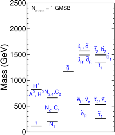
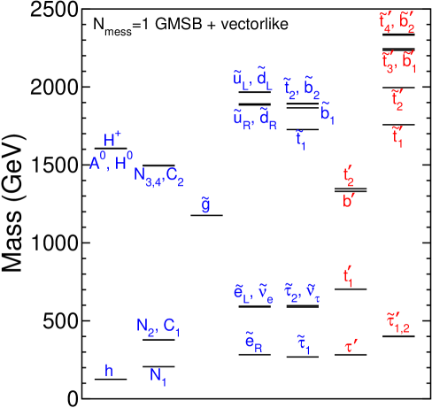
Figure 2.1: The mass spectra for new particles in a minimal GMSB model (left) with light messengers and a similar model with additional chiral supermultiplets in a ${\bf 10}+{\bf\overline{10}}$ of $SU(5)$ (right). In both cases, $M_{\rm mess}=1500$ TeV, $\Lambda=150$ TeV, $\tan\beta=15$, and $\mu>0$. In the model with extra vector-like fields, $k=1$, and $M_{Q}=M_{U}=M_{E}=215$ GeV at the unification scale. The lightest Higgs mass is 114.9 GeV (left) and 124.9 GeV (right).

The minimal GMSB model in the left panel can only manage $M_{h}=115$ GeV, and is therefore clearly ruled out if $M_{h}\sim\!\!125\,{\rm GeV}$. In the right panel, we choose $M_{Q}=M_{U}=M_{E}=215$ GeV at the unification scale, as this leads to $M_{h}=125$ GeV. Comparing the two models, we see that in both cases $M_{\tilde{g}}$ is close to 1160 GeV; this is significant because the gluino mass is the most important parameter pertaining to the discovery of the odd $R$-parity sector at the LHC when squarks are much heavier, as here. However, in this model at least, the lightest new strongly interacting particle is actually the $t_{1}^{\prime}$ with mass near 700 GeV; it is much lighter than the other vector-like quarks $b^{\prime}$ and $t_{2}^{\prime}$, and their superpartners, as well as the MSSM squarks and gluino. The lightest new particle from the ${\bf 10}+{\bf\overline{10}}$ sector is the $\tau^{\prime}$, which if quasi-stable could also be a candidate for the first beyond-the-SM discovery despite lacking strong interactions, as we will discuss below. The model with vector-like supermultiplets also produces squarks that are significantly heavier than the prediction for minimal GMSB. The Higgsino-like neutralinos and charginos $\tilde{N}_{3},\tilde{N}_{4},\tilde{C}_{2}$ are also more than a factor of 2 heavier than the prediction of minimal GMSB, corresponding to a much larger $|\mu|$. If $|\mu|$ is treated as a proxy for the amount of fine tuning in the model, we are forced to accept that the model with extra vector-like supermultiplets is more unnatural than the minimal GMSB model, but this psychological price must be paid if $M_{h}\sim\!\!125\,{\rm GeV}$.

Figure 2.2 shows a similar comparison, but for a much higher messenger scale $M_{\rm mess}=10^{14}$ GeV. The effect of raising the messenger scale is to further increase the squark and slepton masses for the model with extra vector-like matter, both in an absolute sense and compared to the minimal GMSB model. The Higgsino-like neutralinos and charginos are also much heavier in the extended model, pointing to more fine tuning needed in the electroweak symmetry breaking potential, as noted above. For the same input parameters, the gluino mass is suppressed in the extended model on the right compared to the minimal model, but only by about 4%.

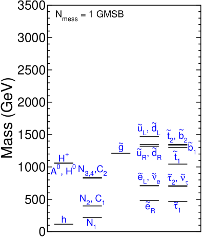
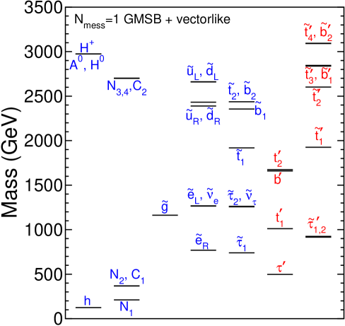
Figure 2.2: As in Figure 2.2, but with very heavy messengers of supersymmetry breaking at $M_{\rm mess}=10^{14}$ GeV. The other parameters are $\Lambda=160$ TeV, $\tan\beta=15$, $\mu>0$, and $k=1$ and $M_{Q}=M_{U}=M_{E}=400$ GeV at the unification scale in the model with extra vector-like particles. The lightest Higgs masses are 115.5 GeV (left) and 124.6 GeV (right).

In both Figures 2.1 and 2.2, the heavier Higgs bosons $A^{0}$, $H^{0}$, and $H^{\pm}$ have their masses substantially increased when the model is extended to include vector-like supermultiplets.

If $\mu M_{2}$ is positive, there will be a positive correction to the anomalous magnetic moment of the muon, bringing the theoretical prediction into better agreement with the experimental result Bennett:2006fi , as has been emphasized in the present context by Endo:2011mc . However, because we are not willing to interpret the present $\sim 3\sigma$ discrepancy as evidence against the SM, we simply take $\mu M_{2}>0$ and do not impose any constraint from $(g-2)_{\mu}$. It is also useful to note that for all models of this type, the effect of the vectorlike quarks is to bring slightly closer agreement with precision electroweak oblique corrections than in the SM, but not by a statistically significant amount Martin:2009bg .

II.3 Achieving $M_{h}\sim\!\!125\,{\rm GeV}$

The corrections to the lightest Higgs mass are most strongly dependent on the masses of $t_{1}^{\prime},t_{2}^{\prime}$ and their superpartners $\tilde{t}_{1,2,3,4}^{\prime}$, with $\Delta M_{h}$ increasing with the hierarchy between the average scalar and fermion masses. The masses of $\tilde{t}_{1,2,3,4}^{\prime}$ scale with the supersymmetry-breaking parameter $\Lambda$, and the smaller they are, the smaller the fermion masses $t_{1,2}^{\prime}$ and $b^{\prime}$ must be in order to accommodate $M_{h}\sim\!\!125\,{\rm GeV}$. The masses of the gluino and $t_{1}^{\prime}$ are of particular interest, since pair production of one of them is likely to give the initial discovery signal at the LHC. Figure 2.3 shows (green sloped funnel) regions in the $M_{t_{1}^{\prime}}$ vs. $M_{\tilde{g}}$ plane in which 122 GeV$<M_{h}<$128 GeV, for $\tan\beta=15$, with $k=1$ at the unification scale. The variation in $M_{\tilde{g}}$ is obtained by varying $\Lambda$, and that of $M_{\tilde{t}_{1}^{\prime}}$ by varying $M_{Q}=M_{U}=M_{E}$ at the unification scale. Three choices of the messenger scale are shown, $M_{\rm mess}=10\Lambda$, $10^{10}$ GeV, and $10^{14}$ GeV.

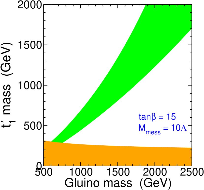
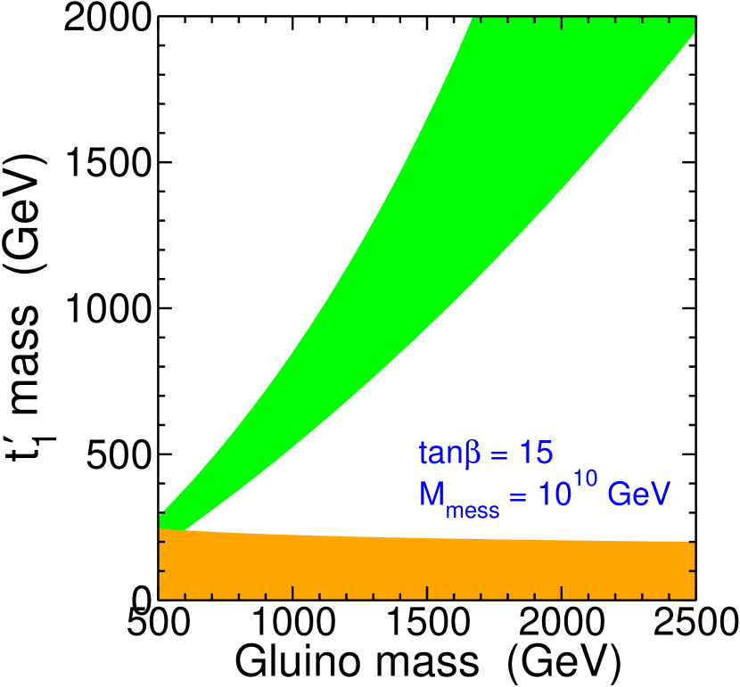
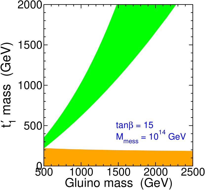
Figure 2.3: Regions in the $M_{t_{1}^{\prime}}$ vs. $M_{\tilde{g}}$ plane for extended GMSB models with a minimal messenger sector and a ${\bf 10}+{\bf\overline{10}}$ of vector-like quarks and leptons, with ${M_{\rm mess}}=10\Lambda$ and $10^{10}$ GeV and $10^{14}$ GeV. The vector-like fermion mass parameters $M_{Q}$ and $M_{U}$ are taken to be unified at the gauge coupling unification scale. The Yukawa coupling $k$ is near its fixed point, obtained by setting $k=1$ at the unification scale, and $\tan\beta=15$. The green sloped funnel regions have a calculated Higgs mass satisfying 122 GeV $<M_{h}<128$ GeV. In the orange shaded region, $M_{\tau^{\prime}}<100$ GeV, assuming that $M_{E}=M_{Q}=M_{U}$ at the unification scale.

Note that, pending exclusions by direct searches for gluino and $t_{1}^{\prime}$, it is easy to obtain $M_{h}\sim\!\!125\,{\rm GeV}$ in this class of models, with $M_{\tilde{g}}$ lower than 700 GeV and $M_{t_{1}^{\prime}}$ lower than 300 GeV even if the messengers are light. Therefore, each new search result at LHC probes an interesting region of parameter space consistent with $M_{h}\sim\!\!125\,{\rm GeV}$, unlike in the usual GMSB models.

The dependence on $\tan\beta$ is shown in Figure 2.4, with allowed regions for $122<M_{h}<128$ GeV in the $\tan\beta$ and $M_{\tilde{g}}$ plane. In each graph, the lighter green curved region furthest right corresponds to the choice of $M_{t^{\prime}_{1}}=1200\,{\rm GeV}$ and the darker green curved region to the left of it corresponds to $M_{t^{\prime}_{1}}=600\,{\rm GeV}$. The upper left triangular red region corresponds to $M_{\tau^{\prime}}<100\,{\rm GeV}$.

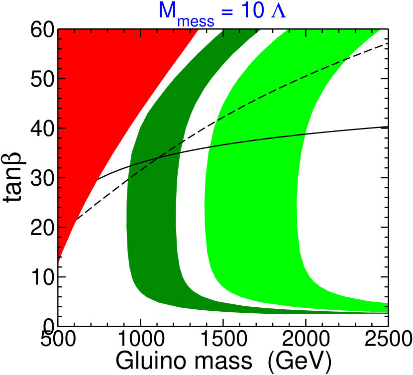
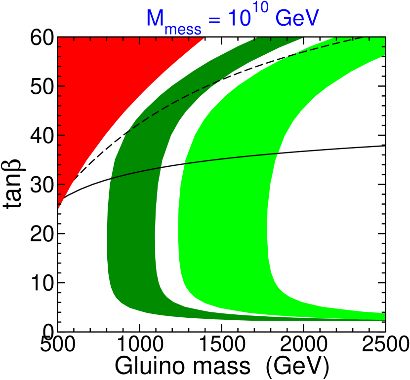
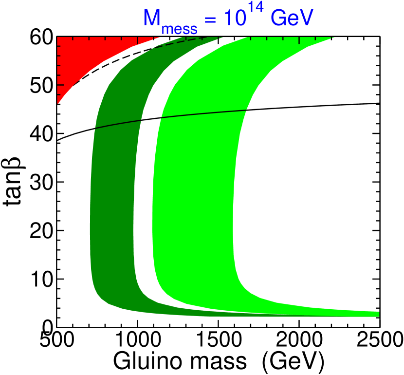
Figure 2.4: Regions in the $\tan\beta$ vs. $M_{\tilde{g}}$ plane with ${M_{\rm mess}}=10\Lambda$ and $10^{10}$ GeV and $10^{14}$ GeV. The vector-like fermion mass parameters $M_{Q},M_{U}$ are taken to be unified at the gauge coupling unification scale. The Yukawa coupling $k$ is near its fixed point, obtained by setting $k=1$ at the unification scale. The green shaded curved regions have a calculated Higgs mass satisfying 122 GeV $<M_{h}<128$ GeV, with the darker green region corresponding to $M_{t_{1}^{\prime}}=600$ GeV and the lighter green region having $M_{t_{1}^{\prime}}=1200$ GeV. In the red shaded region, $M_{\tilde{\tau}_{1}}<100$ GeV. Below (above) the dashed line the NLSP is a neutralino (stau). Above the solid curves, the vacuum is unstable by tunneling to a state with VEVs for the staus, with a liftime shorter than the age of the universe.

The three graphs shown correspond to ${M_{\rm mess}}=10\Lambda$ and $10^{10}$ GeV and $10^{14}$ GeV, and all have $k=1$ at the unification scale. More details regarding underlying parameters are found in the figure caption.

Note that an intermediate value of $10\mathrel{\hbox to0.0pt{\lower 4.0pt\hbox{$\sim$}\hss}\raise 1.0pt\hbox{$<$}}\tan\beta\mathrel{\hbox to0.0pt{\lower 4.0pt\hbox{$\sim$}\hss}\raise 1.0pt\hbox{$<$}}35$ enables a lighter gluino mass, and so lighter MSSM squark masses, than found for $\tan\beta$ outside of that range. For larger $\tan\beta$, the corrections to $M_{h}$ from the tau-stau sector are negative and big, so that larger supersymmetry breaking masses (indicated in the plot by $M_{\tilde{g}}$) are required. For $\tan\beta<10$, the tree-level $M_{h}$ is much smaller, requiring heavier superpartners to obtain $M_{h}\sim\!\!125\,{\rm GeV}$. Similar figures are found in Endo:2011xq ; Endo:2012rd , but with $M_{Q}=M_{U}$ at the TeV scale, rather than at the unification scale as chosen here. An important point Endo:2012rd is that there is an upper bound on $\tan\beta$ in these models, following from the general bound obtained in Hisano:2010re by requiring the standard electroweak-breaking vacuum to be stable (with a lifetime longer than the age of the universe) against tunneling to a vacuum in which the stau fields have VEVs. We show this bound for our models as the solid lines in Figure 2.4. We see again here in this figure that gluino masses easily accessible by LHC now or in the near future are sufficient to deliver a light Higgs boson of mass $\sim\!\!125\,{\rm GeV}$, and this can be achieved for $M_{\tilde{g}}\mathrel{\hbox to0.0pt{\lower 4.0pt\hbox{$\sim$}\hss}\raise 1.0pt\hbox{$<$}}2.5\,{\rm TeV}$ even if $\tan\beta$ is as low as about 3.

As remarked above, $M_{Q}$ and $M_{U}$ are independent in a general theory. Figure 2.5 explores this freedom by showing lines in the $M_{t_{1}^{\prime}},M_{t_{2}^{\prime}}$ plane that predict $M_{h}=125$ GeV, for models with $\tan\beta=15$ and $M_{\rm mess}=10\Lambda$, with the ratio $M_{Q}/M_{U}$ allowed to vary. The special cases with $M_{Q}=M_{U}$ at the unification scale (as in the examples of Figures 2.1, 2.2, 2.3, 2.4 above) are noted by green stars.

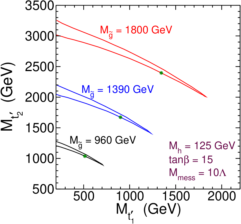
Figure 2.5: Lines in the $M_{t_{1}^{\prime}},M_{t_{2}^{\prime}}$ plane with predicted $M_{h}=125$ GeV, for models with $\tan\beta=15$ and ${M_{\rm mess}}=10\Lambda$, with varying $M_{Q}/M_{U}$. The three lines correspond to $\Lambda=120,180$, and 240 TeV, corresponding to $M_{\tilde{g}}=$ 960, 1390, and $1800\,{\rm GeV}$ respectively. The lower (upper) branch in each case corresponds to $M_{Q}/M_{U}>1$ ($<1$) at the TeV scale. The green stars correspond to $M_{Q}=M_{U}$ at the gauge coupling unification scale.

The three curves correspond to $\Lambda=120,180$, and 240 TeV, resulting in $M_{\tilde{g}}\approx$ 960, 1390, and 1800 respectively. (There is some small variation in the gluino masses on each curve.) We find that for equal values of other parameters, $M_{h}$ remains approximately constant for fixed values of the arithmetic mean of $M_{t_{1}^{\prime}}$ and $M_{t_{2}^{\prime}}$. In particular, the geometric mean is not as good a figure of merit. For each curve in Figure 2.5, we see that there is no minimum value of $M_{t_{1}^{\prime}}$ from the $M_{H}\sim\!\!125\,{\rm GeV}$ constraint alone, because one can always take a very large or small ratio of $M_{Q}/M_{U}$. However, on each curve corresponding to a fixed $M_{\tilde{g}}$, the requirement $M_{h}\sim\!\!125\,{\rm GeV}$ implies a minimum value of $M_{t_{2}^{\prime}}$, and a maximum value of $M_{t_{1}^{\prime}}$.

II.4 Comment on gravitino dark matter

In GMSB models, the LSP is likely to be the gravitino $\tilde{G}$, with mass $M_{\tilde{G}}=\Lambda M_{\rm mess}/\sqrt{3}M_{P}$, where $M_{p}=2.44\times 10^{18}$ GeV. In principle, the gravitino could be a dark matter candidate. One possibility is the gravitino superwimp scenario superwimp in which the gravitino abundance is assumed to be suppressed by a low reheating temperature or diluted by some other non-standard cosmology, followed by the bino-like neutralino LSP freezing out and then decaying out of equilibrium according to $\tilde{N}_{1}\rightarrow\gamma\tilde{G}$, with a lifetime given approximately by Cabibbo:1981er

$$\tau_{\tilde{N}_{1}}=7.5\times 10^{4}\>\mbox{sec}\>\left(\frac{M_{\tilde{G}}}{\mbox{GeV}}\right)^{2}\left(\frac{\mbox{100 GeV}}{M_{\tilde{N}_{1}}}\right)^{5}.$$ (2.13)

If $\tilde{N}_{1}\rightarrow Z\tilde{G}$ is kinematically allowed, then this lifetime is reduced by a factor $1+0.3(1-m_{Z}^{2}/m_{\tilde{N}_{1}}^{2})^{4}$ AKKMM . If the gravitino is to be a significant component of the dark matter, this lifetime should be smaller than about 0.1 to 1 sec, in order that the successful predictions of primordial nucleosynthesis are not affected. This is in tension with a cosmologically relevant relic abundance of gravitinos from decays of thermal binos, given by

$$\Omega_{\tilde{G}}h^{2}=\frac{m_{\tilde{G}}}{m_{\tilde{N}_{1}}}\Omega_{\tilde{N}_{1}}\!h^{2}.$$ (2.14)

Here

$$\Omega_{\tilde{N}_{1}}\!h^{2}\approx 0.013\frac{(1+r)^{4}}{r(1+r^{2})}\left(\frac{m_{\tilde{e}_{R}}}{\mbox{100 GeV}}\right)^{2}\left[1+0.07\ln(\sqrt{r}\,\mbox{100 GeV}/m_{\tilde{e}_{R}})\right]$$ (2.15)

is the relic density of binos that would be found today if they were stable, given in a convenient approximation DMapprox , with $r=m^{2}_{\tilde{N}_{1}}/m^{2}_{\tilde{e}_{R}}$. To illustrate this, we show in Figure 2.6 solid lines of constant $\tau_{\tilde{N}_{1}}=0.1$ and 1 second (relevant for nucleosynthesis) and 1 cm and 1 meter (relevant for collider physics), compared to dashed lines of constant $\Omega_{\tilde{G}}h^{2}=0.11$, $0.01$, and $0.001$, in the $(m_{\tilde{g}},M_{\rm mess})$ plane, with the variation in gluino mass obtained by varying $\Lambda$.

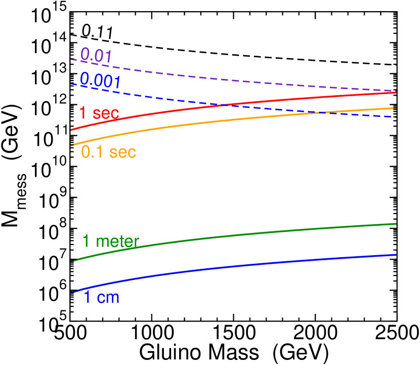
Figure 2.6: Lines of constant NLSP lifetime $\tau_{\tilde{N}_{1}}=1$ second, $0.1$ second, 1 meter, and 1 cm (solid lines), and gravitino abundance resulting from decays of thermal neutralino NLSPs $\Omega_{\tilde{G}}h^{2}=0.11$, $0.01$, and $0.001$ (dashed lines), in the $m_{\tilde{g}}$ and $M_{\rm mess}$ plane. The gluino mass variation was obtained by varying $\Lambda$, with $\tan\beta=15$ and $k=1$.

It is difficult to reconcile gravitino dark matter with the standard picture of primordial nucleosynthesis in this model, without going to very large superpartner masses ($m_{\tilde{g}}\gg 2.5$ TeV), in which case the vector-like quarks would not be necessary and prospects for any discovery of new particles beyond $h^{0}$ at the LHC would be exceedingly grim. Such a massive superpartner spectrum runs counter to the purpose of this paper, which aims to accommodate the $\sim 125\,{\rm GeV}$ with lighter superpartners accessible to the LHC. In the scenario considered in the present paper, these considerations suggest that dark matter is composed mostly of axions or some other particles, with a negligible contribution from gravitinos, and messenger mass scales much above $10^{11}$ GeV are therefore apparently disfavored as indicated in Figure 2.6.

III Masses of exotic quarks and $t_{1}^{\prime}$ decays

Taking into account the full superpotential of the theory $W_{\rm MSSM}+W_{QUE}+W_{\rm mix}$ the fermionic mass matrices for up-type and down-type quarks are Martin:2009bg

$${\cal M}_{u}=\begin{pmatrix}y_{t}v_{u}&\epsilon_{\scriptscriptstyle U}v_{u}&0\cr 0&M_{U}&k^{\prime}v_{d}\cr\epsilon^{\prime}_{\scriptscriptstyle U}v_{u}&kv_{u}&M_{Q}\end{pmatrix},\qquad\quad{\cal M}_{d}=\begin{pmatrix}y_{b}v_{d}&0\cr\epsilon_{\scriptscriptstyle D}v_{d}&\phantom{x}-M_{Q}\end{pmatrix},$$ (3.1)

with mass eigenstates $t,t_{1}^{\prime},t_{2}^{\prime}$ and $b,b^{\prime}$ respectively. The zeros appear as a consequence of a choice of basis. As mentioned earlier, we assume that $\epsilon_{\scriptscriptstyle U}$, $\epsilon^{\prime}_{\scriptscriptstyle U}$, and $\epsilon_{\scriptscriptstyle D}$ can be treated as small perturbations in these mass matrices. Then one always finds $M_{t_{1}^{\prime}}<M_{b^{\prime}}<M_{t_{2}^{\prime}}$, and the exotic quarks will decay according to $t_{2}^{\prime}\rightarrow Wb^{\prime},\>ht_{1}^{\prime},\>Zt_{1}^{\prime}$ and $b^{\prime}\rightarrow W^{(*)}t_{1}^{\prime},\>Wt,\>Zb,\>hb$ and $t_{1}^{\prime}\rightarrow Wb,\>ht,\>Zt$, when kinematically allowed. Formulas for these decays widths, which will be used in our phenomenological discussion below, can be found in Appendix B of Martin:2009bg , and in a more general framework in the Appendix of the present paper.

In Figure 3.1, we plot the mass eigenvalues of the exotic quark states $t^{\prime}_{1,2}$ and $b^{\prime}$ as a function of $M_{Q}/M_{U}$ in the left panel, and the branching fractions of $t_{1}^{\prime}$ vs. $M_{Q}/M_{U}$ in the right panel.

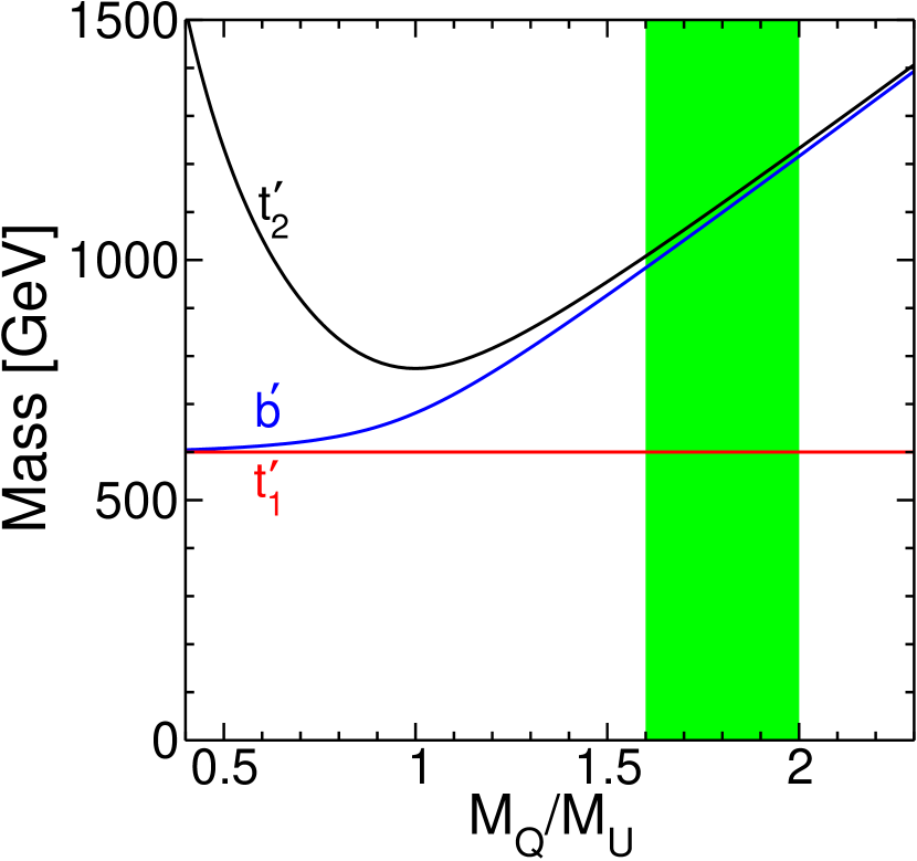
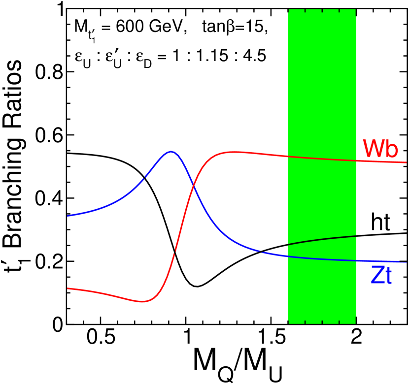
Figure 3.1: Masses (left panel) and $t_{1}^{\prime}$ branching ratios (right panel) for vector-like quarks. Here, $M_{t_{1}^{\prime}}$ is fixed to 600 GeV, and the ratio of mass parameters $M_{Q}$ and $M_{U}$ at the TeV scale is varied. For small (large) $M_{Q}/M_{U}$, the state $t_{1}^{\prime}$ is mostly $SU(2)_{L}$ doublet (singlet). The green band shows the region obtained with the unification condition $M_{Q}=M_{U}$ imposed at the gauge coupling unification scale. The left edge of this band corresponds to $M_{\rm mess}=10^{14}$ GeV, and the right edge to ${M_{\rm mess}}=10\Lambda$. The weak-scale parameters $\epsilon_{\scriptscriptstyle U}$, $\epsilon^{\prime}_{\scriptscriptstyle U}$, and $\epsilon_{\scriptscriptstyle D}$ that describe mixing of the vector-like quarks with the top and bottom quarks are in the ratio $1:1.15:4.5$, which are typical approximate values predicted by requiring them to be unified at the gauge coupling unification scale.

Within this figure $m_{t^{\prime}_{1}}$ is fixed to be $600\,{\rm GeV}$. For $M_{U}\ll M_{Q}$ the $t^{\prime}_{1}$ state is a nearly pure $SU(2)_{L}$-singlet, and it decays into $Wb$, $ht$ and $Zt$ primarily through the interaction $\epsilon_{\scriptscriptstyle U}H_{u}q_{3}\bar{U}$. The dominant decay mode in that limit is to $Wb$ at slightly over 50%, but $ht$ and $Zt$ final states are non-negligible. In the opposite limit $M_{Q}\ll M_{U}$, the state $t^{\prime}_{1}$ is nearly pure $SU(2)_{L}$-doublet, and it decays mostly into $ht$, with $Zt$ a significant subdominant mode. Note that the case $M_{Q}\approx M_{U}$ at the TeV scale is actually in a transition region for the branching ratios. These results were obtained assuming that $\epsilon_{\scriptscriptstyle U}$, $\epsilon^{\prime}_{\scriptscriptstyle U}$ and $\epsilon_{\scriptscriptstyle D}$ are in the low-scale ratios of $1:1.15:4.5$, which are approximate results from assuming they are unified at the gauge coupling unification scale. The thick vertical band in Figure 3.1 indicates the ratio of $M_{Q}/M_{U}$ at the TeV scale under the assumption that $M_{Q}=M_{U}$ at the gauge coupling unification scale (typically in the range $\sim 3$-$8\times 10^{16}\,{\rm GeV}$ for these models). The left edge of this band corresponds to ${M_{\rm mess}}=10^{14}\,{\rm GeV}$, while the right edge of the band corresponds to ${M_{\rm mess}}=10\Lambda$.

It is also interesting to consider the dependence on the mixing couplings $\epsilon_{\scriptscriptstyle U}$, $\epsilon^{\prime}_{\scriptscriptstyle U}$, and $\epsilon_{\scriptscriptstyle D}$, because the relation eq. (2.12) may not hold. This is illustrated in Figure 3.2, in which we hold fixed $M_{Q}/M_{U}=1.8$, and vary $\epsilon^{\prime}_{\scriptscriptstyle U}/\epsilon_{\scriptscriptstyle U}$ with $\epsilon_{\scriptscriptstyle D}=0$, and $\epsilon_{\scriptscriptstyle D}/\epsilon_{\scriptscriptstyle U}$ with $\epsilon^{\prime}_{\scriptscriptstyle U}=0$. When the ratio $|\epsilon^{\prime}_{\scriptscriptstyle U}/\epsilon_{\scriptscriptstyle U}|$ is less than a few, and when $\epsilon_{\scriptscriptstyle D}/\epsilon_{\scriptscriptstyle U}\mathrel{\hbox to0.0pt{\lower 4.0pt\hbox{$\sim$}\hss}\raise 1.0pt\hbox{$<$}}50$, one recovers results similar to the unification-motivated results given in Figure 3.1.

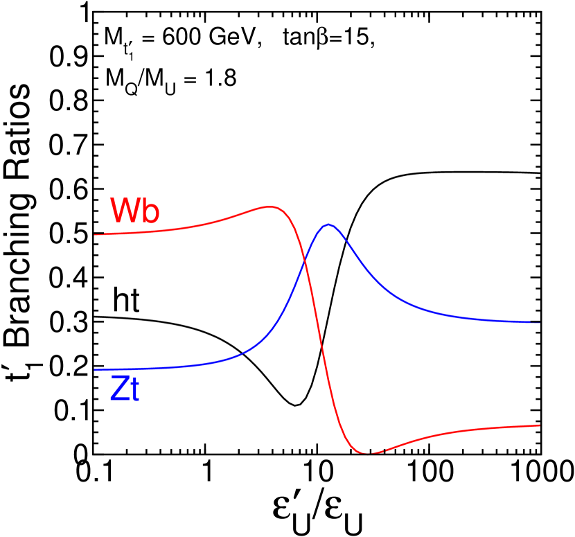
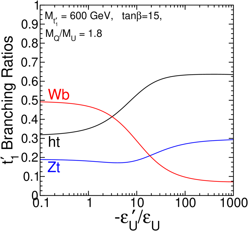
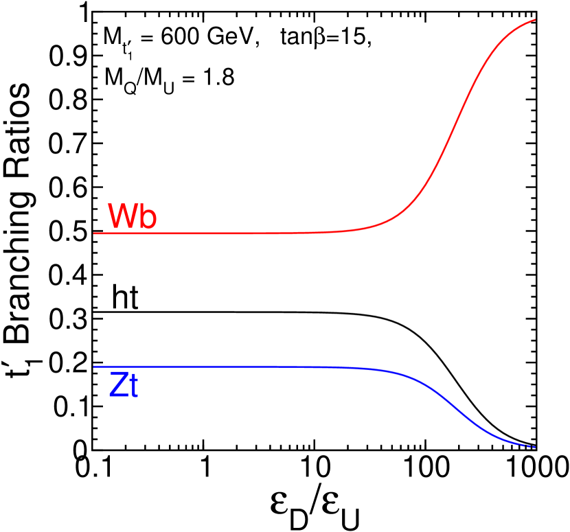
Figure 3.2: Branching ratios for $t_{1}^{\prime}$ as a function of ratios of the mixing couplings. In the top two panels, the ratio $\epsilon^{\prime}_{\scriptscriptstyle U}/\epsilon_{\scriptscriptstyle U}$ is varied over positive (left panel) and negative (right panel) values, with $\epsilon_{\scriptscriptstyle D}=0$. In the lower panel, the ratio $\epsilon_{\scriptscriptstyle D}/\epsilon_{\scriptscriptstyle U}$ is varied, with $\epsilon^{\prime}_{\scriptscriptstyle U}=0$. (The results do not depend on the sign of the ratio in the latter case.)

This is because in that case the effects of $\epsilon_{\scriptscriptstyle U}$ are dominant because of the $SU(2)_{L}$-singlet nature of $t_{1}^{\prime}$. However, for larger values of $\epsilon^{\prime}_{\scriptscriptstyle U}$, one enters a “$W$-phobic” regime for $t_{1}^{\prime}$ in which the $ht$ final state can dominate with B$(Wb)$ very small. Conversely, for $\epsilon_{\scriptscriptstyle D}$ very large, one goes over into the charged-current dominated case that B$(Wb)=1$, which coincides with the prediction for a sequential $t^{\prime}$, the subject of most experimental searches. Clearly, it is crucial that experimental searches go beyond this case, to take into account and hopefully exploit the $ht$ and $Zt$ final states.

The dependence of these branching ratios on the magnitude of the $t_{1}^{\prime}$ mass is mild provided that it is well above the $W,Z,h$ masses. This is illustrated in Figure 3.3, which shows the branching fractions of $t^{\prime}_{1}$ as a function of its mass, keeping fixed $k=1$ and using the unified boundary conditions $M_{Q}=1.8M_{U}$ and $\epsilon_{\scriptscriptstyle U}:\epsilon^{\prime}_{\scriptscriptstyle U}:\epsilon_{\scriptscriptstyle D}=1:1.15:4.5$.

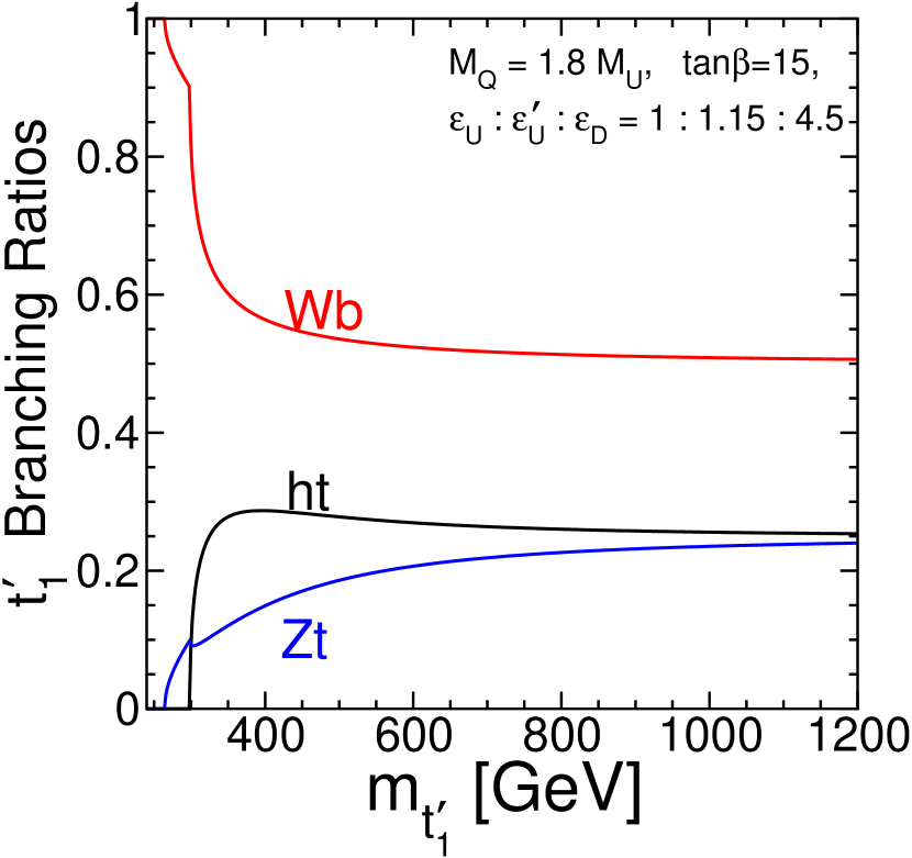
Figure 3.3: Branching ratios for $t_{1}^{\prime}$ as a function of its mass, obtained with $M_{Q}=1.8M_{U}$ and $\epsilon_{\scriptscriptstyle U}:\epsilon^{\prime}_{\scriptscriptstyle U}:\epsilon_{\scriptscriptstyle D}=1:1.15:4.5$.

For low $t_{1}^{\prime}$ masses $\mathrel{\hbox to0.0pt{\lower 4.0pt\hbox{$\sim$}\hss}\raise 1.0pt\hbox{$<$}}400$ GeV, the branching fractions show some variation, but with higher $t_{1}^{\prime}$ mass they asymptote to B$(Wb)=50\%$, B$(ht)=25\%$, and B$(Zt)=25\%$, but with $\mbox{B}(ht)>\mbox{B}(Zt)$ for finite masses relevant to the LHC.

IV Precision tests from mixing with third-family fermions

The introduction of an additional $b^{\prime}$ quark that mixes with the third generation $b$ quark can induce a tree-level shift in the $Z$ boson coupling to the right-handed $b$ quark mass eigenstate compared to the SM. Such a shift is very severely constrained by the measurement of $R_{b}$ at LEP Bamert:1996px , with

$$R_{b}^{expt}=0.21629\pm 0.00066$$ (4.2)

from LEPEWWG . The SM computed best fit value is LEPEWWGupdate ; LEPEWWG

$$R_{b}^{SM}=0.21579\pm 0.00013.$$ (4.3)

Thus, the $3\sigma$ range of allowed shifts in $R_{b}$ compared to the SM value is

$$-0.0015<\delta R_{b}<0.0025,$$ (4.4)

where $\delta R_{b}\equiv R_{b}-R_{b}^{SM}$. From eqs. (A.9) and (A.10) in the Appendix, and relating the coupling conventions in LEPEWWGupdate ; LEPEWWG to ours by $g^{b}_{L}\equiv(c_{W}/g)g^{Z}_{d^{\dagger}_{3}d_{3}}$ and $g^{b}_{R}\equiv-(c_{W}/g)g^{Z}_{\bar{d}^{\dagger}_{3}\bar{d}_{3}}$, we see that the tree-level shifts in the couplings are

$$\delta g^{b}_{L}=0,\qquad\qquad\delta g^{b}_{R}=-\frac{1}{2}|R^{\prime}_{43}|^{2}\approx-\frac{\epsilon_{\scriptscriptstyle D}^{2}v^{2}\cos^{2}\beta}{2m^{2}_{b^{\prime}}},$$ (4.5)

which shows that the mixing always reduces the magnitude of the right-handed $b$ quark couplings to the $Z$ boson. With this definition the resulting shift in $R_{b}$ is Bamert:1996px

$$R_{b}=R_{b}^{SM}(1+0.645\,\delta g_{R}^{b})$$ (4.6)

which implies that the $3\sigma$ range of allowed $\delta g_{R}^{b}$ is

$$-0.011<\delta g_{R}^{b}<0.018.$$ (4.7)

Thus the requirement that $R_{b}$ is in 3-$\sigma$ agreement with experiment gives a constraint on $\epsilon_{\scriptscriptstyle D}$, $\tan\beta$ and $m_{b^{\prime}}$. From eqs. (4.5) and (4.7) we find the requirement that

$$|\epsilon_{\scriptscriptstyle D}|<0.42\,\tan\beta\,\left(\frac{m_{b^{\prime}}}{500\,{\rm GeV}}\right)\sqrt{1+\frac{1}{\tan^{2}\beta}}.$$ (4.8)

A similar analysis follows from considering shifts in ${\cal A}_{b}$ and $A_{FB}^{b}$. The current LEPEWWG ; LEPEWWGupdate experimental situation is that

$${\cal A}_{b}^{expt}=0.923\pm 0.020~{}~{}~{}{\rm and}~{}~{}~{}A_{FB}^{b,expt}=0.0992\pm 0.0016,$$ (4.9)

whereas the SM computed best fit values are

$${\cal A}_{b}^{SM}=0.9346\pm 0.0001~{}~{}~{}{\rm and}~{}~{}~{}A_{FB}^{b,SM}=0.1033\pm 0.0008.$$ (4.10)

Let us focus on $A^{b}_{FB}$, as the SM prediction is $2.8\sigma$ too high compared to the measurement (see table 8.4 of LEPEWWG ).

From the definition $A_{FB}\equiv(g^{2}_{L}-g_{R}^{2})/(g^{2}_{L}+g^{2}_{R})$ one can compute the shift in $A^{b}_{FB}$ from a shift in $g_{R}^{b}$ to be

$$A_{FB}^{b}=A_{FB}^{b,SM}(1-1.7\,\delta g_{R}^{b})~{}~{}~{}\Longrightarrow~{}~{}~{}\delta A_{FB}^{b}=-0.18\,\delta g_{R}^{b}.$$ (4.11)

Since $\delta g_{R}^{b}<0$, this implies that the shift in the prediction of $A_{FB}^{b}$ is always positive, increasing the tension between theory and experiment. If we therefore assume that the $b-b^{\prime}$ mixing is no more than a $1\sigma$ effect in the “wrong” direction (i.e., $\delta A_{FB}^{b}<0.0016$ from $b-b^{\prime}$ mixing), this puts a limit on $\delta g_{R}^{b}$ that translates to exactly the same formula as eq. (4.8) except that $0.42$ is replaced by $0.38$. Thus, the constraints on $b^{\prime}$ mixing are not very severe as long as $m_{b^{\prime}}$ is greater than a few hundred GeV or $\tan\beta$ is not small.

Another way to constrain the mixing of SM third-family quarks with the exotic quarks is through the CKM matrix element $V_{tb}$. Here, we cannot assume unitarity of the CKM matrix, since it will not be in general [see eq. (A.13) in the Appendix]. If the $\epsilon_{\scriptscriptstyle D}$ coupling is present simultaneously with the $\epsilon_{\scriptscriptstyle U}$ or $\epsilon^{\prime}_{\scriptscriptstyle U}$ couplings, then the situation is complicated by the fact that the $W$ boson will have small couplings to right-handed SM quarks as well as left-handed quarks. For the sake of illustration, consider the case that only $\epsilon_{\scriptscriptstyle U}$ is important, and suppose that the SM Yukawa coupling matrices are such that if $\epsilon_{\scriptscriptstyle U}$ were exactly 0, then $V_{tb}$ would be very close to 1 (as one finds in the SM with CKM unitarity assumed), so that all mixing of the first two families with the third family and the vector-like quarks can be neglected. With those assumptions, from eq. (A.13) we obtain

$$1-V_{tb}\approx 0.06\,\epsilon_{\scriptscriptstyle U}^{2}\sin^{2}\beta\left(\frac{\mbox{500 GeV}}{M_{U}}\right)^{2},$$ (4.12)

This can be compared to the values obtained from single top production without assuming CKM unitarity, $V_{tb}=0.88\pm 0.07$ (from Tevatron singletop ) and $V_{tb}=1.04\pm 0.09$ (from CMS CMSsingletop ). Thus, even if $\epsilon_{\scriptscriptstyle U}$ is near unity and $t_{1}^{\prime}$ is not much heavier than its experimental bound, the CKM constraint does not impact the model.

Next, we consider the implications of $\tau-\tau^{\prime}$ mixing. This mixing will induce a positive shift in the $g_{L}^{\tau}\equiv(g/c_{W})g^{Z}_{e^{\dagger}_{3}e_{3}}$ coupling to the $Z$ boson, while $g_{R}^{\tau}\equiv-(g/c_{W})g^{Z}_{\bar{e}^{\dagger}_{3}\bar{e}_{3}}$ is unaffected. From eqs. (A.29) and (A.30),

$$\delta g_{L}^{\tau}=\frac{1}{2}|U_{43}|^{2}\approx\frac{\epsilon_{\scriptscriptstyle E}^{2}v^{2}\cos^{2}\beta}{2m^{2}_{\tau^{\prime}}},\qquad\qquad\delta g_{R}^{\tau}=0.$$ (4.13)

An important effect that results from this shift is an alteration in the $A_{\tau}$ observable. From the definition $A_{\ell}=(g_{L}^{2}-g_{R}^{2})/(g_{L}^{2}+g_{R}^{2})$, the shift in $\delta A_{\tau}$ from a shift in $\delta g_{L}^{\tau}$ is

$$A_{\tau}=A_{\tau}^{SM}(1-23\,\delta g_{L}^{\tau})$$ (4.14)

which demonstrates the high sensitivity to changes in the $\tau$ lepton couplings to the $Z$.

The experimental and theoretical values LEPEWWG of $A_{\tau}$ are

$$A^{expt}_{\tau}(P_{\tau})=0.1465\pm 0.0033~{}~{}~{}{\rm and}~{}~{}~{}A^{SM}_{\tau}(P_{\tau})=0.1480\pm 0.0011.$$ (4.15)

Keeping the prediction to within $3\sigma$ of the experimental measurement requires that $-0.0120<\delta A_{\tau}<0.0090$. Since $\delta A_{\tau}$ is always negative from the $\tau^{\prime}$ mixing, the lower limit is the applicable constraint. From eq. (4.14) we see that $\delta g^{\tau}_{L}<0.0033$, or

$$|\epsilon_{\scriptscriptstyle E}|<0.23\,\tan\beta\,\left(\frac{m_{\tau^{\prime}}}{500\,{\rm GeV}}\right)\,\sqrt{1+\frac{1}{\tan^{2}\beta}}.$$ (4.16)

This requirement is not terribly constraining, especially considering that the SM $\tau$ Yukawa coupling $y_{\tau}=0.01$ is much smaller than the general constraints on $\epsilon_{E}$ when $m_{\tau^{\prime}}>100\,{\rm GeV}$.

Finally, one can attempt to constrain the $\tau$-$\tau^{\prime}$ mixing through the $\tau$ decay measurement. The analysis of SwainTaylor corresponds to $|U_{43}|^{2}<0.0053$ in the notation of the Appendix of the present paper, which therefore implies the same constraint as eq. (4.16) but with $0.21$ replacing $0.23$. However, this is a 1-$\sigma$ constraint. Also, this assumes that the PMNS matrix is unitary, and that mixing in the electron and muon sectors is absent, which need not hold Lacker:2010zz . In any case, there is no impact on the coupling $\epsilon_{\scriptscriptstyle E}$ in this model unless $\tan\beta$ is small, and the $\tau^{\prime}$ is light.

V LHC phenomenology

The exotic quarks could in principle have a significant effect on the production and decay of the lightest Higgs boson. For an additional chiral fourth family, which relies entirely on Yukawa couplings for its large masses, there is a very large positive effect on the production cross-section sigmahfourthfamily ; KPST , in strong conflict with the current limits ATLAScombined ; CMScombined . However, in the vector-like model under present consideration, the situation is very different. The corrections to the $hgg$ and $h\gamma\gamma$ effective interactions can be found from the general formulas in Ishiwata:2011hr . Applying these, we find that for the case $k^{\prime}\ll k\approx 1$, these corrections are totally negligible. Even if $k^{\prime}$ is sizable, the corrections to $gg\rightarrow h\rightarrow\gamma\gamma$ are quite modest, at most at the 5% level for $M_{t_{1}^{\prime}}=500$ GeV and $\tan\beta=5$ and $k=1$, $k^{\prime}=0.7$, and can have either sign depending on the relative phases in the $t_{1}^{\prime},t_{2}^{\prime},b^{\prime}$ sector mass matrices. For larger $\tan\beta$, the size of the effect decreases. We conclude that at least for LHC physics in the short term, the loop effects of the exotic quarks on Higgs production and decay are probably too small to hope to observe.

The model under consideration differs from other variants of the MSSM in that there are two distinct paths to a new physics discovery. First, we may discover the odd $R$-parity superpartners of the SM states. Second, we have the exotic quark and lepton states. These two possibilities are essentially decoupled, and it is unclear which of them should provide the initial discovery of physics beyond the SM, since the masses and decays are negotiable within the general model framework. We will begin by commenting on features of the superpartner phenomenology at LHC, making the comparison to other standard searches.

V.1 Superpartner signals

If the NLSP is a neutralino $(\tilde{N}_{1})$ that is stable on detector-crossing time scales, the resulting phenomenology is very similar to “standard supersymmetry” signatures (e.g., mSUGRA). The squarks are comparatively heavy, with up and down squarks, which play the most important role in LHC production, between about 1.6 and 2.3 times heavier than the gluino (see for example Figures 2.1, 2.2). Therefore, the discovery potential comes mostly from gluino pair production, gluino+squark production, or the production of wino-like charginos and neutralinos, followed in each case by decays to jets, leptons and large missing energy. The production cross-sections computed to next-to-leading order by Prospino prospino are shown in Figure 5.1 for the most important processes $pp\rightarrow\tilde{g}\tilde{g}$ and $\tilde{g}\tilde{Q}+\tilde{g}\tilde{\overline{Q}}$ and $\tilde{C}_{1}^{\pm}\tilde{N}_{2}$ and $\tilde{C}_{1}^{+}\tilde{C}_{1}^{-}$.

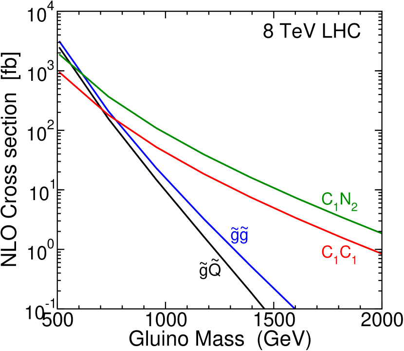
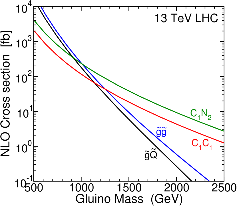
Figure 5.1: NLO production cross-sections for $\tilde{g}\tilde{g}$ and $\tilde{g}\tilde{Q}+\tilde{g}\tilde{\overline{Q}}$ and $\tilde{C}_{1}^{\pm}\tilde{N}_{1}$ and $\tilde{C}_{1}\tilde{C}_{1}$, as a function of the gluino mass, for GMSB models with extra vector-like quarks in this paper with ${M_{\rm mess}}=10\Lambda$ and $\tan\beta=15$, in $pp$ collisions with $\sqrt{s}=8$ and 13 TeV.

Here we used a model line with ${M_{\rm mess}}=10\Lambda$, $\tan\beta=15$, $k=1$, and $\mu>0$, but the dependence on these particular assumptions is mild, with the exception of $\tilde{g}\tilde{Q}+\tilde{g}\tilde{\overline{Q}}$, which becomes smaller for a given $M_{\tilde{g}}$ if ${M_{\rm mess}}$ is larger. Although the gluino+gluino and gluino+squark pair production cross-section are smaller than the chargino-neutralino rates for $M_{\tilde{g}}\mathrel{\hbox to0.0pt{\lower 4.0pt\hbox{$\sim$}\hss}\raise 1.0pt\hbox{$>$}}650$ GeV at $\sqrt{s}=8$ TeV, and for $M_{\tilde{g}}\mathrel{\hbox to0.0pt{\lower 4.0pt\hbox{$\sim$}\hss}\raise 1.0pt\hbox{$>$}}1050$ GeV at $\sqrt{s}=13$ TeV, the gluino and squark signals should have higher acceptances due to more visible energy. However, any attempts to probe much beyond $M_{\tilde{g}}=1$ TeV at $\sqrt{s}=8$ TeV may have to rely on chargino/neutralino production rather than gluino/squark production.

The branching ratios of the gluino are, for the typical low-${M_{\rm mess}}$ model in Figure 2.1:

$$\tilde{g} \rightarrow jj\tilde{C}_{1}\>\>(\mbox{38\%}),\qquad tb\,\tilde{C}_{1}\>\>(\mbox{17\%}),\qquad jj\tilde{N}_{2}\>\>(\mbox{19\%}),\qquad bb\tilde{N}_{2}\>\>(\mbox{6\%}),$$ (5.1)

$$tt\tilde{N}_{2}\>\>(\mbox{3\%}),\qquad jj\tilde{N}_{1}\>\>(\mbox{12\%}),\qquad bb\tilde{N}_{1}\>\>(\mbox{1\%}),\qquad tt\tilde{N}_{1}\>\>(\mbox{4\%}),$$

from SDECAY SDECAY , where $j$ denotes a jet from a $u,d,s,c$ quark, and the notation omits the distinction between quarks and antiquarks. Up and down squarks essentially always decay to a gluino and a very energetic jet. The wino-like charginos and neutralinos decay almost entirely through the lighter stau, which then decays as $\tilde{\tau}_{1}\rightarrow\tau\tilde{N}_{1}$ with a branching ratio of 100%:

$$\tilde{C}_{1} \rightarrow \tilde{\tau}_{1}\nu\rightarrow\tau\nu\tilde{N}_{1}\>\>\>(\mbox{96\%}),\qquad W\tilde{N}_{1}\>\>(\mbox{4\%}),$$ (5.2)

$$\tilde{N}_{2} \rightarrow \tilde{\tau}_{1}\tau\rightarrow\tau^{+}\tau^{-}\tilde{N}_{1}\>\,\>(\mbox{96\%}),\qquad h\tilde{N}_{1}\>\>(\mbox{4\%}),$$ (5.3)

Thus a high proportion of events will have 2, 3, or 4 taus in the final state, manifested either as hadronic tau jets or softer $e,\mu$. This is an important difference compared to mSUGRA, where comparable models with such heavy squarks have large $m_{0}$ and therefore also have heavy staus, and so cannot produce such a predominance of taus in the final state.

In contrast, models with higher ${M_{\rm mess}}$ will have $M_{\tilde{\tau}_{1}}>M_{\tilde{C}_{1}}\approx M_{\tilde{N}_{2}}$, as illustrated by the example in Figure 2.2, implying a much lower tau multiplicity. In that example model, we have for the gluino decays

$$\tilde{g} \rightarrow jj\tilde{C}_{1}\>\>(\mbox{33\%}),\qquad tb\,\tilde{C}_{1}\>\>(\mbox{18\%}),\qquad jj\tilde{N}_{2}\>\>(\mbox{16\%}),\qquad bb\tilde{N}_{2}\>\>(\mbox{6\%}),$$ (5.4)

$$tt\tilde{N}_{2}\>\>(\mbox{3\%}),\qquad jj\tilde{N}_{1}\>\>(\mbox{13\%}),\qquad bb\tilde{N}_{1}\>\>(\mbox{2\%}),\qquad tt\tilde{N}_{1}\>\>(\mbox{9\%}),$$

similar to eq. (5.1), with a slightly higher average number of $b$ jets. However, the wino-like charginos and neutralinos decay very differently than in the low-$M_{\rm mess}$ case:

$$\tilde{C}_{1} \rightarrow W\tilde{N}_{1}\>\>(\mbox{100\%}),$$ (5.5)

$$\tilde{N}_{2} \rightarrow h\tilde{N}_{1}\>\>(\mbox{97\%}),\qquad Z\tilde{N}_{1}\>\>(\mbox{3\%}).$$ (5.6)

This means that over 40% of gluino pair production events, and almost all $\tilde{C}_{1}\tilde{N}_{2}$ events, will have a Higgs boson in them. For such models with $M_{\tilde{\tau}_{1}}>M_{\tilde{C}_{1}}\approx M_{\tilde{N}_{2}}$, the signals are sufficiently similar to mSUGRA ones with large $m_{0}$ that one can safely approximate the limits by those obtained by ATLAS and CMS for the same gluino mass and heavier squarks. The ratios of squark masses to the gluino mass are shown for our model in Figure 5.2.

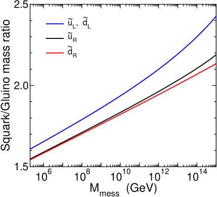
Figure 5.2: The ratio of the first-family squark masses to the mass of the gluino, as a function of $M_{\rm mess}$. Here, $\tan\beta=15$, $\mu>0$, and $\Lambda=160$ TeV.

These squark/gluino mass ratios correspond approximately to CMSSM models with $m_{0}/M_{1/2}$ ranging from about 3.4 (for low ${M_{\rm mess}}$) to 5.2 (for high ${M_{\rm mess}}$). At present, the LHC limits for these large $m_{0}$ cases imply only $M_{\tilde{g}}\mathrel{\hbox to0.0pt{\lower 4.0pt\hbox{$\sim$}\hss}\raise 1.0pt\hbox{$>$}}850$ GeV from ATLASSUSYlargem0 ; CMSSUSYlargem0 . A direct comparison is hindered somewhat by the fact that the LHC collaborations unfortunately choose to present results for the CMSSM in terms of the unphysical input variables $(m_{0},M_{1/2})$ rather than physical gluino and squark masses.

Because of the importance of the transition in parameter space between the cases that $\tilde{\tau}_{1}$ is lighter or heavier than the wino-like neutralinos and charginos, we show in Figure 5.3 how the ratio $M_{\tilde{\tau}_{1}}/M_{\tilde{C}_{1}}$ behaves as a function of $M_{\rm mess}$ for various values of $\tan\beta$.

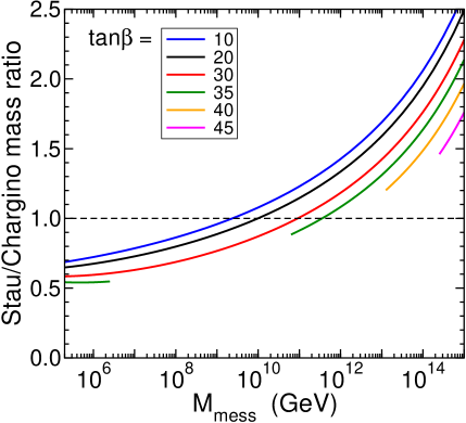
Figure 5.3: The ratio $M_{\tilde{\tau}_{1}}/M_{\tilde{C}_{1}}$ of the lighter stau and chargino masses, as a function of $M_{\rm mess}$, for $\tan\beta=10,20,30,35,40,45$. Here, $\Lambda=160$ TeV and $\mu>0$. The missing parts of the lines for $\tan\beta=35,40,45$ are due to the vacuum stability requirement.

For $M_{\tilde{\tau}_{1}}/M_{\tilde{C}_{1}}\mathrel{\hbox to0.0pt{\lower 4.0pt\hbox{$\sim$}\hss}\raise 1.0pt\hbox{$<$}}1$, the decays $\tilde{C}_{1}\rightarrow\tilde{\tau}_{1}\nu$ and $\tilde{N}_{2}\rightarrow\tilde{\tau}_{1}\tau$ dominate; otherwise, decays to $W$ and $h$ dominate. Depending on $\tan\beta$, we see from Figure 5.3 that the transition between these two regimes occurs at an intermediate scale of a few times $10^{9}$ to a few times $10^{11}$ GeV.

If the decay $\tilde{N}_{1}\rightarrow\gamma\tilde{G}$ is prompt, then the above event topologies will be supplemented by two energetic isolated photons, for which SM backgrounds are quite low. This would increase the discovery potential dramatically, and would probably guarantee that the discovery would happen in the $\tilde{C}_{1}\tilde{N}_{2}$ production channel, due to its larger cross-section. Because the NLSP decay width is proportional to $1/F^{2}$, where $F\mathrel{\hbox to0.0pt{\lower 4.0pt\hbox{$\sim$}\hss}\raise 1.0pt\hbox{$>$}}\Lambda{M_{\rm mess}}$, we see from Figure 5.3 that the prompt neutralino NLSP decay signal should be $\tau\tau\tau\gamma\gamma+E_{T}^{\rm miss}$, where $\tau$ can be either a softer lepton or a hadronic tau jet.

Another possibility is that the NLSP is the lighter stau, which can only occur in our model framework if $\tan\beta$ is large. (However, $\tan\beta$ cannot be too large, and $M_{\rm mess}$ must be low, given the constraints on vacuum stability evident in Figure 2.4.) In that case, all superpartner decays chains will terminate in $\tilde{\tau}_{1}\rightarrow\tau\tilde{G}$, where $\tilde{G}$ is the goldstino (gravitino). In each decay chain from a gluino, chargino, or neutralino parent, lepton flavor conservation dictates that there is another $\tau$ produced. This means that if the NLSP stau decay is prompt, essentially all supersymmetric events will have at least 4 taus, while if it is not prompt, one has at least 2 taus and 2 quasi-stable staus which can be detected as slow-moving heavy charged particles. However, the parameter space in which there is a stau NLSP is limited, as one runs into the constraint from stability of the vacuum noted in Hisano:2010re ; Endo:2012rd . For example, in the models of Figure 2.4, one sees that this requires a low ${M_{\rm mess}}$, and $M_{\tilde{g}}<1100$ GeV, and $21<\tan\beta<34$.

V.2 Search for $t_{1}^{\prime}$ at the LHC

The production cross-sections for generic exotic heavy quarks at the LHC are shown in Figure 5.4, for various $\sqrt{s}$ values.

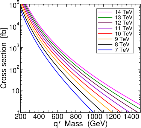
Figure 5.4: The production cross-section in $pp$ collisions for an exotic quark-antiquark pair $\sigma(q^{\prime}\bar{q}^{\prime})$ as a function of its mass $M_{q^{\prime}}$, for $\sqrt{s}=7,8,9,10,11,12,13,14$ TeV, obtained using HATHOR HATHOR .

The collider phenomenology of the $t^{\prime}_{1}$ depends crucially on whether it decays promptly or not. If the mixing between the exotic quarks and the SM quarks is very small, then there is a chance that $t_{1}^{\prime}$ could be stable on time scales relevant for collider detectors. Assuming first the unification ratio $M_{Q}/M_{U}=1.8$, so that $t_{1}^{\prime}$ is mostly $SU(2)_{L}$ singlet, we find a lifetime for $t^{\prime}_{1}$ of

$$c\tau=\left(\frac{\mbox{1000 GeV}}{M_{t_{1}^{\prime}}}\right)\left(\frac{10^{-7}}{\epsilon}\right)^{2}\times\left\{\begin{array}[]{ll}\mbox{0.94 mm}&{\rm for}\>\,\epsilon=\epsilon_{\scriptscriptstyle U}\sin\beta,\>\>\>\epsilon^{\prime}_{\scriptscriptstyle U}=\epsilon_{\scriptscriptstyle D}=0,\\[-5.0pt] \mbox{290 mm}&{\rm for}\>\,\epsilon=\epsilon^{\prime}_{\scriptscriptstyle U}\sin\beta,\>\>\>\epsilon_{\scriptscriptstyle U}=\epsilon_{\scriptscriptstyle D}=0,\\[-5.0pt] \mbox{340 mm}&{\rm for}\>\,\epsilon=\epsilon_{\scriptscriptstyle D}\cos\beta,\>\>\>\epsilon_{\scriptscriptstyle U}=\epsilon^{\prime}_{\scriptscriptstyle U}=0.\end{array}\right.$$ (5.10)

For simplicity, we have taken the limit $M_{t_{1}^{\prime}}^{2}\gg M_{h}^{2}$ in eq. (5.10). For masses closer to the weak boson masses, kinematic factors increase the lifetime somewhat. To illustrate the opposite limit of the $t_{1}^{\prime}$ being mostly an $SU(2)_{L}$ doublet, consider $M_{Q}=0.5M_{U}$, which results in

$$c\tau=\left(\frac{\mbox{1000 GeV}}{M_{t_{1}^{\prime}}}\right)\left(\frac{10^{-7}}{\epsilon}\right)^{2}\times\left\{\begin{array}[]{ll}\mbox{270 mm}&{\rm for}\>\,\epsilon=\epsilon_{\scriptscriptstyle U}\sin\beta,\>\>\>\epsilon^{\prime}_{\scriptscriptstyle U}=\epsilon_{\scriptscriptstyle D}=0,\\[-5.0pt] \mbox{1.8 mm}&{\rm for}\>\,\epsilon=\epsilon^{\prime}_{\scriptscriptstyle U}\sin\beta,\>\>\>\epsilon_{\scriptscriptstyle U}=\epsilon_{\scriptscriptstyle D}=0,\\[-5.0pt] \mbox{2.0 mm}&{\rm for}\>\,\epsilon=\epsilon_{\scriptscriptstyle D}\cos\beta,\>\>\>\epsilon_{\scriptscriptstyle U}=\epsilon^{\prime}_{\scriptscriptstyle U}=0.\end{array}\right.$$ (5.14)

If we require for the definition of prompt decays that $c\tau<1$ mm, then we need only either $\epsilon_{\scriptscriptstyle U}$ or $\epsilon^{\prime}_{\scriptscriptstyle U}$ to be greater than a few times $10^{-7}$ to ensure prompt decays. Note that the $\epsilon_{\scriptscriptstyle D}$ contribution to the inverse lifetime is suppressed by $\cos^{2}\beta$.

Let us first assume the case of $t^{\prime}_{1}$ decaying promptly. The LHC experiments have several analyses based on the production of heavy top-like quarks. The most stringent direct search bounds are from CMS, but are limited to the extreme cases that either the $Wb$ or the $Zt$ final state dominates. For $B(t^{\prime}\rightarrow Wb)=1$, CMS obtains $M_{t^{\prime}}>557$ GeV using 4.7 fb^-1 CMStprimeWb , and for $B(t^{\prime}\rightarrow Zt)=1$, they obtain $M_{t^{\prime}}>475$ GeV using 1.14 fb^-1 CMStprimeZt . However, in our case the branching ratios are split among the final states depending on the mixing couplings, as seen in Figures 3.1-3.3. In much of parameter space, where $M_{t^{\prime}_{1}}>$ few hundred GeV and $M_{Q}>M_{U}$, we find $B(t^{\prime}_{1}\to bW)\approx 50\%$. Therefore, requiring $t^{\prime}_{1}\bar{t}^{\prime}_{1}\to bWbW$ means a reduction by a factor of 4 in total cross-section applicable for the analysis. Taking this factor into account, and comparing the cross-section limits at LHC as derived in Halk:2012 with the total direct rate in our theory assuming $B(t^{\prime}_{1}\to bW)=50\%$, we extrapolate to find the current limit to be $M_{t^{\prime}_{1}}\mathrel{\hbox to0.0pt{\lower 4.0pt\hbox{$\sim$}\hss}\raise 1.0pt\hbox{$>$}}420$, even without using the other final states. This is consistent with another recent analysis RaoWhiteson . In Figure 5.5 we show the limits as a function of $B(t^{\prime}_{1}\to bW)$ based on the $t^{\prime}_{1}\bar{t}^{\prime}_{1}\to bWbW$ limits only.

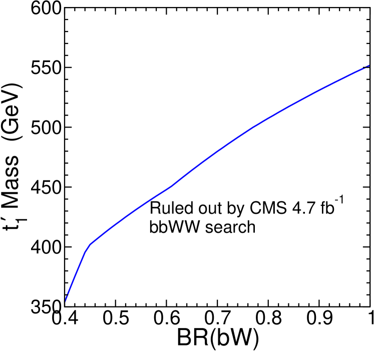
Figure 5.5: Limits on $m_{t^{\prime}_{1}}$ vs. B$(t^{\prime}_{1}\to bW)$, from the CMS search for the final state $bbWW$ based on 4.7^-1 fb reported in Halk:2012 .

Of course, a more general search using all three final states $Wb$, $Zt$ and $ht$ will find a stronger limit. In ref. RaoWhiteson a reanalysis of these direct search limits together with a reinterpretation of an ATLAS search ATLASbprimeWt for $b^{\prime}\rightarrow Wt$ in terms of $t^{\prime}$ pair production is argued to give a bound $M_{t_{1}^{\prime}}>415$ GeV, for any combination of the three branching ratios for $t^{\prime}\rightarrow Wb,Zt,Zh$. Going forward, the detector collaborations should strive to incorporate all three final states in their search strategies as much as possible, in order to maximize the model-independent reach in the $t_{1}^{\prime}$ mass. For any value of $M_{t_{1}^{\prime}}$, the mixing couplings can be chosen in such a way that any of the $Wb$, $Zt$, or $ht$ is the dominant decay mode, and they may all be comparable to each other. This should be kept in mind in the planning and interpretation of hadron collider searches. Even if $t^{\prime}\rightarrow Wb$ has the largest branching ratio, searches with mixed final states $(t^{\prime}\rightarrow Wb)(t^{\prime}\rightarrow Zt)$ or $(t^{\prime}\rightarrow Wb)(t^{\prime}\rightarrow ht)$ may give the strongest signal, exploiting the presence of $Z\rightarrow\ell^{+}\ell^{-}$ and 2, 3, or 4 $b$-tagged jets, or even $h\rightarrow b\overline{b}$ or $h\rightarrow\tau^{+}\tau^{-}$ with a “known” invariant mass of $\sim\!\!125\,{\rm GeV}$. This is especially important given that there are other, completely different, new physics models that predict exotic quarks within the reach of the LHC LittleHiggs -Geller:2012wx , which can span the possible branching ratios into these three final states. It would be especially interesting to observe and study events with $h\rightarrow b\bar{b}$ or $h\rightarrow\tau^{+}\tau^{-}$ in $t_{1}^{\prime}$ production, since these decay modes are quite difficult to observe at the LHC from direct Higgs production.

If the $t^{\prime}_{1}$ is stable, it can be searched for as a strongly interacting heavy stable charged particle. The implications for the search are expected to be similar to that of a quasi-stable top squark when, for example, it is the NLSP and the decay to gravitino is very suppressed and the lifetime is greater than the size of the detector, $c\tau>\ell_{\rm detector}$. The search strategy CMS-11-022 relies on first identifying large $dE/dx$ energy depositions in the inner tracker due to the massive stable charged particle traversing it. This combined with the requirement of high $p_{T}$ is the so-called tracker method of discovery. In addition the excellent timing of the muon system enables a time-of-flight cut, since a massive particle will have smaller velocity usually than a muon and thus takes more time to reach the outer muon chambers. The combination of these two methods, tracker and time-of-flight, yields powerful constraints from the $\sqrt{s}=7\,{\rm TeV}$ data. With $4.7\,{\rm fb}^{-1}$ of integrated luminosity, we can compare the cross-section vs. mass limits of Halk:2012 to the cross-section computation in Figure 5.4, and from extrapolation of these results conclude that there is a limit of quasi-stable $t^{\prime}_{1}$ mass of $m_{t^{\prime}_{1}}\mathrel{\hbox to0.0pt{\lower 4.0pt\hbox{$\sim$}\hss}\raise 1.0pt\hbox{$>$}}950\,{\rm GeV}$. We estimate that more than twice this sensitivity could be achieved at $14\,{\rm TeV}$ LHC with more than $10\,{\rm fb}^{-1}$ of integrated luminosity.

V.3 Search for $b^{\prime}$ at the LHC

In addition to the $t_{1}^{\prime}$, the ${\bf 10}+\overline{\bf 10}$ model has exotic quarks $b^{\prime}$ and $t_{2}^{\prime}$. It is of particular interest to ask what are the sensitivities to $b^{\prime}$ production at the LHC Gopalakrishna:2011ef , since its mass may be nearly that of the $t^{\prime}_{1}$ fermion when $M_{Q}<M_{U}$, as seen in Figure 3.1. Given that its production rate is nearly the same as that of a similar mass $t^{\prime}_{1}$, due to QCD contributions dominating, we must ask how the LHC would find this state, which is almost pure $SU(2)_{L}$-doublet in both its right- and left-handed components.

The $b^{\prime}$ can have two-body decays through the mixing parameters $\epsilon_{\scriptscriptstyle U}$, $\epsilon^{\prime}_{\scriptscriptstyle U}$, or $\epsilon_{\scriptscriptstyle D}$ to possible final states $Wt$, $Zb$ and $hb$. Again, we are assuming that the exotic fermions couple only to the third generation weak eigenstates in order to tame potential flavor problems in the theory. The decay widths are calculated (in the more general case of arbitrary mixing with the SM quarks) in the Appendix, eqs. (A.15)-(A.17). The relative fraction of the decays into $Wt$ versus $Zb$ and $ht$ depends to a large extent on the ratio $\epsilon_{\scriptscriptstyle D}/(\epsilon^{\prime}_{\scriptscriptstyle U}\tan\beta)$. If this ratio is smaller than 1, or if $\epsilon_{\scriptscriptstyle D}/\epsilon_{\scriptscriptstyle U}$ is small, then $b^{\prime}$ yields mostly $Wt$, if kinematically accessible. If the ratio is larger than 1, then the $b^{\prime}$ yields mostly $Zb$ and $hb$. The branching ratios are shown in Figure 5.6 for a nearly pure doublet $b^{\prime}$, as a function of $\epsilon_{\scriptscriptstyle D}/\epsilon_{\scriptscriptstyle U}$ with $\epsilon^{\prime}_{\scriptscriptstyle U}=1.1\epsilon_{\scriptscriptstyle U}$ and $\epsilon_{\scriptscriptstyle U}$ = 0.

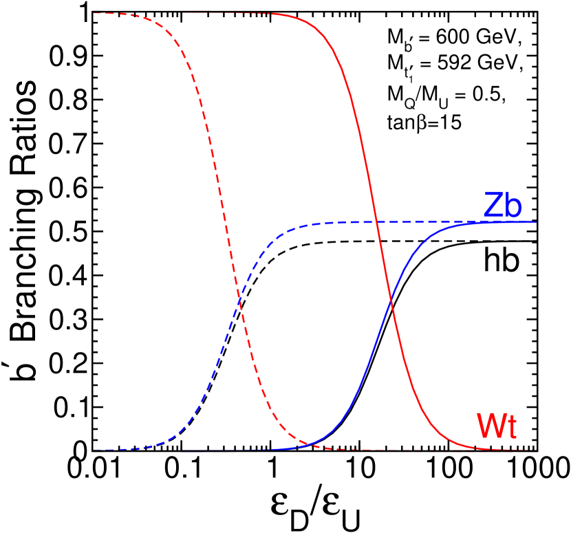
Figure 5.6: Branching ratios for a nearly pure $SU(2)_{L}$ doublet $b^{\prime}$ into $Wt$, $Zb$, and $hb$, as a function of $\epsilon_{\scriptscriptstyle D}/\epsilon_{\scriptscriptstyle U}$. Here $M_{Q}=600$ GeV and $M_{U}=1200$ GeV with $k=1$, so that $m_{b^{\prime}}=600$ GeV and $m_{t_{1}^{\prime}}=592$ GeV. The solid lines have $\epsilon^{\prime}_{\scriptscriptstyle U}=1.1\epsilon_{\scriptscriptstyle U}$, and the dashed lines have $\epsilon^{\prime}_{\scriptscriptstyle U}=0$. The three-body decay $b^{\prime}\rightarrow t_{1}^{\prime}f\overline{f}$ through an off-shell $W$ boson is highly suppressed by kinematics, and is assumed to have a small branching ratio.

It is also necessary to consider the flavor-preserving decay $b^{\prime}\rightarrow W^{(*)}t_{1}^{\prime}$. If $M_{b^{\prime}}>M_{t_{1}^{\prime}}+M_{W}$, then this is an on-shell two-body decay and it will dominate. However, for the case that $b^{\prime}$ is mostly doublet, the decay will be three-body with the $W$ boson off shell. The formula for this decay width is found in the Appendix, eq. (A.18). In Figure 5.7, we show this width for the idealized case that $b^{\prime}$ has pure doublet couplings to $W$ and $t_{1}^{\prime}$, as a function of the mass difference $M_{b^{\prime}}-M_{t_{1}^{\prime}}$, which is the most crucial parameter.

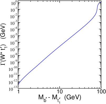
Figure 5.7: The decay width $\Gamma(b^{\prime}\rightarrow W^{(*)}t_{1}^{\prime})$ as a function of the mass difference $M_{b^{\prime}}-M_{t_{1}^{\prime}}$, assuming that $b^{\prime}$ and $t_{1}^{\prime}$ form a nearly unmixed $SU(2)_{L}$ doublet, for $M_{b^{\prime}}=500$ GeV. (The results for the range 400 GeV $<M_{b^{\prime}}<$ 1000 GeV are visually nearly indistinguishable from the line shown on this graph.)

For comparison, the two-body flavor-violating decay widths are approximately:

$$\Gamma_{b^{\prime}} = \mbox{0.1 GeV}\left(\frac{M_{b^{\prime}}}{\mbox{1000 GeV}}\right)\left(\frac{\epsilon}{0.1}\right)^{2}$$ (5.15)

for the cases $\epsilon=\epsilon^{\prime}_{\scriptscriptstyle U}\sin\beta$, $\epsilon_{\scriptscriptstyle D}=\epsilon_{\scriptscriptstyle U}=0$ and $\epsilon=\epsilon_{\scriptscriptstyle D}\cos\beta$, $\epsilon_{\scriptscriptstyle U}=\epsilon^{\prime}_{\scriptscriptstyle U}=0$, and

$$\Gamma_{b^{\prime}}=9\times 10^{-5}\>\mbox{GeV}\left(\frac{M_{b^{\prime}}}{\mbox{1000 GeV}}\right)\left(\frac{\mbox{1000 GeV}}{M_{U}}\right)^{4}\left(\frac{\epsilon_{\scriptscriptstyle U}\sin\beta}{0.1}\right)^{2}$$ (5.16)

for $\epsilon^{\prime}_{\scriptscriptstyle U}=\epsilon_{\scriptscriptstyle D}=0$. Thus, the decay $b^{\prime}\rightarrow W^{(*)}t_{1}^{\prime}$ may or may not dominate in this case, with a strong dependence on both the mass difference and the mixing couplings.

If $b^{\prime}$ mostly decays into $Wt$ the current limits arise from a search by CMS CMSbprimeWt based on 4.9 fb^-1 of integrated luminosity, resulting in a limit $M_{b^{\prime}}>611$ GeV if $B(b^{\prime}\rightarrow Wt)=1$. For a $b^{\prime}$ quark decaying only into $Zb$, there is an ATLAS search ATLASbprimeZb based on 2.0 fb^-1 which results in $M_{b^{\prime}}>400$ GeV. In our case, we see from Figure 5.6 that $B(b^{\prime}\rightarrow Zb)=0.5$ is a more likely scenario, in which case the limit from ATLASbprimeZb is about 360 GeV. However, the ATLAS analysis only uses $Z\rightarrow e^{+}e^{-}$, so improvements can be expected both from using $\mu^{+}\mu^{-}$ and more integrated luminosity. As in the case of $t_{1}^{\prime}$, it would be useful to exploit the other decay modes in a comprehensive search strategy that allows the branching ratios to vary. In particular, the decay $b^{\prime}\rightarrow hb$ will lead to a nice signal in which there are at least 4 potentially taggable $b$-jets. For example $pp\rightarrow b^{\prime}\bar{b}^{\prime}\rightarrow(Zb)(hb)\rightarrow\ell^{+}\ell^{-}bbbb$ should make for a background-free signal.

V.4 Search for $\tau^{\prime}$ at the LHC

The spectrum of the model we are considering also has an exotic lepton, the $\tau^{\prime}$, whose quantum numbers are those of a right-handed electron with its vector complement. If the $\tau^{\prime}$ decays promptly, it will be difficult to find. Assuming that mixing is only with the $\tau$, the branching ratios to final states $W\nu$, $Z\tau$ and $h\tau$ are shown in Figure 5.8.

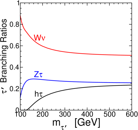
Figure 5.8: The branching ratio of $\tau^{\prime}$ into the final states $W\nu$, $Z\tau$, and $h\tau$, as a function of its mass, assuming $M_{h}=125$ GeV.

The total width is determined by the $\epsilon_{\scriptscriptstyle E}$ coupling in eq. (2.6), but the branching ratios depend only on the $\tau^{\prime}$ mass. The production cross-section is rather low for this state, being electroweak strength, as is shown in Figure 5.9.

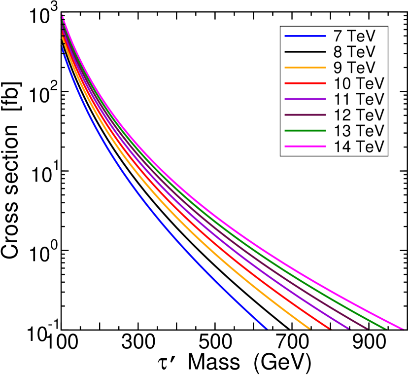
Figure 5.9: The total production cross-section $\sigma(\tau^{\prime+}\tau^{\prime-})$ as a function of $m_{\tau^{\prime}}$, for $\sqrt{s}=$7, 8, 9, 10, 11, 12, 13, 14 TeV.

However, one can produce unique signatures such as $\ell^{+}\tau^{-}h+E_{T}^{\rm miss}$ that could be exploited at the LHC to simultaneously find the Higgs boson and the $\tau^{\prime}$. A full exploration of these prospects will be pursued in another publication.

If the $\tau^{\prime}$ is stable, it can be searched for as a weakly interacting heavy stable charged particle. The lifetime depends only on the mass and on the mixing coupling $\epsilon_{\scriptscriptstyle E}$, with

$$c\tau=\left(\frac{\mbox{1000 GeV}}{M_{\tau^{\prime}}}\right)\left(\frac{10^{-7}}{\epsilon_{\scriptscriptstyle E}\cos\beta}\right)^{2}\mbox{1.0 mm}.$$ (5.17)

We have taken the formal limit of $M_{\tau^{\prime}}\gg M_{h},M_{Z},M_{W}$ here for simplicity, and kinematic effects will lengthen $c\tau$ by a factor of a few if the $\tau^{\prime}$ mass is not far above 100 GeV. Note that there is also an enhancement of the lifetime proportional to $1/\cos^{2}\!\beta$, so that the $\tau^{\prime}$ could have a measurable decay length with $\epsilon_{\scriptscriptstyle E}$ as large as a few times $10^{-5}$ if $\tan\beta$ is large. While this may seem quite small, it is larger than the electron Yukawa coupling in the SM.

The implications for the search are like that of a quasi-stable stau boson NLSP. The search strategies are very similar to that described in the $t^{\prime}$ section above, and so we shall not repeat it here. The result is that with $4.7\,{\rm fb}^{-1}$ of integrated luminosity, we can compare the cross-section vs. mass limits of Halk:2012 to the cross-section computation in Figure 5.9, and conclude that there is a limit of quasi-stable $\tau^{\prime}$ mass of $m_{\tau^{\prime}}\mathrel{\hbox to0.0pt{\lower 4.0pt\hbox{$\sim$}\hss}\raise 1.0pt\hbox{$>$}}450\,{\rm GeV}$. We estimate that with $100\,{\rm fb}^{-1}$ of integrated luminosity at a $14\,{\rm TeV}$ LHC phase, the reach for quasi-stable $\tau^{\prime}$ can extend up to nearly $1\,{\rm TeV}$, which is well within the range of $\tau^{\prime}$ masses expected for $M_{h}\sim\!\!125\,{\rm GeV}$ assuming that $M_{E}=M_{Q}=M_{U}$ at the unification scale, as illustrated by the examples of Figures 2.1 and 2.2.

VI Conclusion

A minimal GMSB model, with one $SU(5)$ ${\bf 5}+\overline{\bf 5}$ messenger pair, can explain a Higgs mass of $\sim\!\!125\,{\rm GeV}$ with even a sub-TeV gluino. This is accomplished by adding to the spectrum ${\bf 10}+\overline{\bf 10}$ vector-like states, which then couple to the Higgs boson via the superpotential of eq. (2.5). The resulting radiative corrections can easily add 10 GeV or more to the light Higgs boson mass, which is crucial to achieve the $\sim\!\!125\,{\rm GeV}$ naturally, without requiring superpartners to be well above $1\,{\rm TeV}$ or invoking ad hoc non-GMSB stop mixing. We have paid special attention to cases inspired by unification of masses, $M_{Q}=M_{U}$, and mixing couplings, $\epsilon_{\scriptscriptstyle U}=\epsilon^{\prime}_{\scriptscriptstyle U}=\epsilon_{\scriptscriptstyle D}$, and we have characterized its parameter space. In this case, it is generic that the lightest exotic quark of the spectrum, $t^{\prime}_{1}$, is mostly that with quantum numbers similar to right-handed top quark, with particular decay branching fractions.

The most obvious implication for this scenario is the existence of low-scale supersymmetry that should reveal itself at the LHC in the coming years. The searches for superpartners should follow the usual searches for GMSB models, which implies the existence of standard supersymmetry missing energy signatures with the addition of extra photons (or taus) if the NLSP is a neutralino (or stau) and decays promptly. The signals may feature also either the presence of the lightest Higgs boson $h$ or a high multiplicity of taus due to wino decays in many events, depending on the messenger scale. If the decays of the NLSP are not prompt, the collider phenomenology will be similar to that of standard scenarios with the neutralino being the LSP (i.e., stable NLSP on detector time scales), or there will be stable charged particle tracks from a quasi-stable charged NLSP stau.

The scenario under consideration in this paper yields additional phenomenological implications due to the existence of the $t^{\prime}_{1,2}$ and $b^{\prime}$ and $\tau^{\prime}$ exotic fermion states. In previous sections we have explained that these states can also yield quasi-stable charged particle tracks, with sensitivity being nearly $1\,{\rm TeV}$ already for $t^{\prime}_{1}$ and nearly $0.5\,{\rm TeV}$ for $\tau^{\prime}$. If the decays are prompt, the limits are reduced. In that case the $t^{\prime}_{1}$ pair-production signal is probably the most telling one for our scenario. We estimate sensitivity to the $t^{\prime}_{1}$ mass to be higher than $1800\,{\rm GeV}$ at 14 TeV LHC with more than $10\,{\rm fb}^{-1}$ of integrated luminosity. If seen with the properties described in the previous sections, the signal would point to the existence of extra vector-like quarks that lift the Higgs boson mass to $\sim\!\!125\,{\rm GeV}$.

Appendix: Exotic quark and lepton couplings to $W,Z,h$ and decay widths

This Appendix is devoted to a systematic description of the interactions of quarks and leptons to the massive weak bosons $W,Z,h$, allowing for arbitrary flavor violation, and to formulas for the corresponding flavor-violating fermion decays.

In the quark sector, we promote the third-family mixing parameters $\epsilon_{\scriptscriptstyle U}$, $\epsilon^{\prime}_{\scriptscriptstyle U}$, and $\epsilon_{\scriptscriptstyle D}$ to couplings $\epsilon^{\scriptscriptstyle U}_{i}$, $\epsilon^{\scriptscriptstyle U\prime}_{i}$, and $\epsilon^{\scriptscriptstyle D}_{i}$ respectively, where the index $i=1,2,3$ indicates the three SM generations. The masses for up-type and down-type quarks in the gauge-eigenstate basis are then respectively $5\times 5$ and $4\times 4$ matrices:

$${\cal M}_{u}=\begin{pmatrix}y^{u}_{ij}v_{u}&\epsilon^{\scriptscriptstyle U}_{i}v_{u}&0\cr 0&M_{U}&k^{\prime}v_{d}\cr\epsilon^{\scriptscriptstyle U\prime}_{j}v_{u}&kv_{u}&M_{Q}\end{pmatrix},\qquad\quad{\cal M}_{d}=\begin{pmatrix}y^{d}_{ij}v_{d}&0\cr\epsilon^{\scriptscriptstyle D}_{j}v_{d}&\phantom{x}-M_{Q}\end{pmatrix},$$ (A.1)

where $y^{u}_{ij}$ and $y^{d}_{ij}$ are the $3\times 3$ MSSM Yukawa couplings for the ordinary quarks, and the 0 entries appear by a choice of basis. One can now obtain the gauge-eigenstate two-component left-handed fermions by applying unitary rotation matrices $L$, $R$, $L^{\prime}$ and $R^{\prime}$ on the mass eigenstates $u_{i}=(u,c,t,t_{1}^{\prime},t_{2}^{\prime})$ and $\overline{u}_{i}=(\overline{u},\overline{c},\overline{t},\overline{t}_{1}^{\prime},\overline{t}_{2}^{\prime})$, and $d_{i}=(d,s,b,b^{\prime})$ and $\overline{u}_{i}=(\overline{d},\overline{s},\overline{b},\overline{b}^{\prime})$, so that

$$L^{T}{\cal M}_{u}R = \mbox{diag}(m_{u},m_{c},m_{t},m_{t_{1}^{\prime}},m_{t_{2}^{\prime}}),$$ (A.2)

$$L^{\prime T}{\cal M}_{d}R^{\prime} = \mbox{diag}(m_{d},m_{s},m_{b},m_{b^{\prime}}).$$ (A.3)

The first index of each of $L,R,L^{\prime},R^{\prime}$ is a gauge eigenstate index, and the second is a mass eigenstate index. Then the interaction Lagrangian for couplings of $W,Z,h$ to the quarks can be written as

$$-{\cal L}_{\rm int} = W_{\mu}^{+}\Bigl{(}g^{W}_{u_{i}^{\dagger}d_{j}}\,u^{\dagger}_{i}\overline{\sigma}^{\mu}d_{j}\,+\,g^{W}_{\overline{d}^{\dagger}_{i}\overline{u}_{j}}\,\overline{d}^{\dagger}_{i}\overline{\sigma}^{\mu}\overline{u}_{j}\Bigr{)}+W_{\mu}^{-}\Bigl{(}g^{W}_{d_{j}^{\dagger}u_{i}}\,d^{\dagger}_{j}\overline{\sigma}^{\mu}u_{i}\,+\,g^{W}_{\overline{u}^{\dagger}_{j}\overline{d}_{i}}\,\overline{u}^{\dagger}_{j}\overline{\sigma}^{\mu}\overline{d}_{i}\Bigr{)}$$ (A.4)

$$+Z_{\mu}\Bigl{(}g^{Z}_{u^{\dagger}_{i}u_{j}}\,u^{\dagger}_{i}\overline{\sigma}^{\mu}u_{j}\,+\,g^{Z}_{\overline{u}^{\dagger}_{i}\overline{u}_{j}}\,\overline{u}^{\dagger}_{i}\overline{\sigma}^{\mu}\overline{u}_{j}\,+\,g^{Z}_{d^{\dagger}_{i}d_{j}}\,d^{\dagger}_{i}\overline{\sigma}^{\mu}d_{j}\,+\,g^{Z}_{\overline{d}^{\dagger}_{i}\overline{d}_{j}}\,\overline{d}^{\dagger}_{i}\overline{\sigma}^{\mu}\overline{d}_{j}\Bigr{)}$$

$$+\Bigl{(}y^{h}_{u_{i}\overline{u}_{j}}h^{0}u_{i}\overline{u}_{j}+y^{h}_{d_{i}\overline{d}_{j}}h^{0}d_{i}\overline{d}_{j}+{\rm c.c.}\Bigr{)},$$

where the couplings for the $W$ boson are

$$g^{W}_{u_{i}^{\dagger}d_{j}}=\bigl{(}g^{W}_{d_{j}^{\dagger}u_{i}}\bigr{)}^{*} = \frac{g}{\sqrt{2}}\biggl{(}\sum_{k=1}^{3}L_{ki}^{*}L^{\prime}_{kj}+L_{5i}^{*}L^{\prime}_{4j}\biggr{)},$$ (A.5)

$$g^{W}_{\overline{d}^{\dagger}_{i}\overline{u}_{j}}=\bigl{(}g^{W}_{\overline{u}^{\dagger}_{j}\overline{d}_{i}}\bigr{)}^{*} = \frac{g}{\sqrt{2}}R_{4i}^{\prime*}R_{5j},$$ (A.6)

and the couplings for the $Z$ boson are

$$g^{Z}_{u^{\dagger}_{i}u_{j}} = \frac{g}{c_{W}}\biggl{[}\Bigl{(}\frac{1}{2}-\frac{2}{3}s_{W}^{2}\Bigr{)}\delta_{ij}-\frac{1}{2}L^{*}_{4i}L_{4j}\biggr{]},$$ (A.7)

$$g^{Z}_{\overline{u}^{\dagger}_{i}\overline{u}_{j}} = \frac{g}{c_{W}}\biggl{(}\frac{2}{3}s_{W}^{2}\delta_{ij}-\frac{1}{2}R^{*}_{5i}R_{5j}\biggr{)},$$ (A.8)

$$g^{Z}_{d^{\dagger}_{i}d_{j}} = \frac{g}{c_{W}}\Bigl{(}-\frac{1}{2}+\frac{1}{3}s_{W}^{2}\Bigr{)}\delta_{ij},$$ (A.9)

$$g^{Z}_{\overline{d}^{\dagger}_{i}\overline{d}_{j}} = \frac{g}{c_{W}}\biggl{(}-\frac{1}{3}s_{W}^{2}\delta_{ij}+\frac{1}{2}R^{\prime*}_{4i}R^{\prime}_{4j}\biggr{)},$$ (A.10)

and the couplings for the lightest Higgs scalar boson are

$$y^{h}_{u_{i}\overline{u}_{j}} = \frac{1}{\sqrt{2}}\cos\alpha\Bigl{(}L_{ki}R_{nj}y^{u}_{kn}+L_{ki}R_{4j}\epsilon^{\scriptscriptstyle U}_{k}+L_{5i}R_{nj}\epsilon^{\scriptscriptstyle U\prime}_{n}+L_{5i}R_{4j}k\Bigr{)}-\frac{1}{\sqrt{2}}\sin\alpha\,L_{4i}R_{5j}k^{\prime},\phantom{xxx}$$ (A.11)

$$y^{h}_{d_{i}\overline{d}_{j}} = -\frac{1}{\sqrt{2}}\sin\alpha\,\Bigl{(}L^{\prime}_{ki}R^{\prime}_{nj}y^{d}_{kn}+L^{\prime}_{4i}R^{\prime}_{nj}\epsilon^{\scriptscriptstyle D}_{n}\Bigr{)}.$$ (A.12)

The couplings to the heavier neutral Higgs bosons $H^{0}$ and $A^{0}$ are obtained by the replacements $(\cos\alpha,\sin\alpha)\rightarrow(\sin\alpha,-\cos\alpha)$ and $(i\cos\beta,-i\sin\beta)$ respectively.

Note that in the couplings of the $W$ boson in eq. (A.5), the role of the SM CKM matrix is played by the restriction to the $i,j=1,2,3$ subspace of the $5\times 4$ matrix

$$K_{ij}=\sum_{k=1}^{3}L_{ki}^{*}L^{\prime}_{kj}+L_{5i}^{*}L^{\prime}_{4j}.$$ (A.13)

Clearly, neither the full matrix $K_{ij}$ nor its restriction is unitary. (In the standard notation of RPP , our $K_{11}$ is $V_{ud}$, our $K_{23}$ is $V_{cb}$, etc.) Also, there is a nonzero coupling of the $W$ boson to right-handed quarks in eq. (A.6), unlike in the SM. However, these flavor-violating effects do decouple as $\epsilon^{\scriptscriptstyle U}_{i}$, $\epsilon^{\scriptscriptstyle U\prime}_{i}$ and $\epsilon^{\scriptscriptstyle D}_{i}$ are taken to zero or as $M_{Q}$ and $M_{U}$ are taken very large. Similarly, tree-level flavor-changing neutral currents of the $Z$ boson couplings appear as the three terms with explicit reference to the exotic quarks’ gauge-eigenstate indices $4,5$ in eqs. (A.7), (A.8), and (A.10).

The widths of kinematically allowed flavor-changing two-body decays of quarks involving weak bosons are given by

$$\Gamma(u_{i}\rightarrow Wd_{j}) = \frac{M_{u_{i}}}{32\pi}\lambda^{1/2}(1,r_{W},r_{j})\Bigl{\{}[1+r_{j}-2r_{W}+(1-r_{j})^{2}/r_{W}](|g^{W}_{u^{\dagger}_{i}d_{j}}|^{2}+|g^{W}_{\overline{u}_{i}^{\dagger}\overline{d}_{j}}|^{2})$$ (A.14)

$$+12\sqrt{r_{j}}\,{\rm Re}[g^{W}_{u^{\dagger}_{i}d_{j}}g^{W}_{\overline{u}_{i}^{\dagger}\overline{d}_{j}}]\Bigr{\}},$$

$$\Gamma(d_{i}\rightarrow Wu_{j}) = \frac{M_{d_{i}}}{32\pi}\lambda^{1/2}(1,r_{W},r_{j})\Bigl{\{}[1+r_{j}-2r_{W}+(1-r_{j})^{2}/r_{W}](|g^{W}_{u^{\dagger}_{j}d_{i}}|^{2}+|g^{W}_{\overline{u}_{j}^{\dagger}\overline{d}_{i}}|^{2})$$ (A.15)

$$+12\sqrt{r_{j}}\,{\rm Re}[g^{W}_{u^{\dagger}_{j}d_{i}}g^{W}_{\overline{u}_{j}^{\dagger}\overline{d}_{i}}]\Bigr{\}},$$

$$\Gamma(q_{i}\rightarrow Zq_{j}) = \frac{M_{q_{i}}}{32\pi}\lambda^{1/2}(1,r_{Z},r_{j})\Bigl{\{}[1+r_{j}-2r_{Z}+(1-r_{j})^{2}/r_{Z}](|g^{Z}_{q^{\dagger}_{i}q_{j}}|^{2}+|g^{Z}_{\overline{q}_{i}^{\dagger}\overline{q}_{j}}|^{2})$$ (A.16)

$$+12\sqrt{r_{j}}\,{\rm Re}[g^{Z}_{q^{\dagger}_{i}q_{j}}g^{Z}_{\overline{q}_{i}^{\dagger}\overline{q}_{j}}]\Bigr{\}},$$

$$\Gamma(q_{i}\rightarrow hq_{j}) = \frac{M_{q_{i}}}{32\pi}\lambda^{1/2}(1,r_{h},r_{j})\Bigl{\{}[1+r_{j}-r_{h}](|y^{h}_{q_{i}\overline{q}_{j}}|^{2}+|y^{h}_{q_{j}\overline{q}_{i}}|^{2})+4\sqrt{r_{j}}\,{\rm Re}[y^{h}_{q_{i}\overline{q}_{j}}y^{h}_{q_{j}\overline{q}_{i}}]\Bigr{\}},\phantom{xxxx}$$ (A.17)

with $q=u$ or $d$, and $\lambda(x,y,z)=x^{2}+y^{2}+z^{2}-2xy-2xz-2yz$, and $r_{X}=M_{X}^{2}/M_{q_{i}}^{2}$. The special cases considered in the text above are $t_{1}^{\prime}\rightarrow Wb,Zt,ht$, and $b^{\prime}\rightarrow Wt,Zb,hb$, both obtained by taking $i=4$ and $j=3$, with the mixing of exotic quarks to SM quarks restricted to the third family. The $t_{1}^{\prime}$ decays were also discussed in Martin:2009bg (using a different notation).

In the case of a $b^{\prime}$ with $M_{b^{\prime}}<M_{t_{1}^{\prime}}+M_{W}$, there may be a competition between the two-body decays above and the flavor-preserving three-body decay through an off-shell $W$ boson to SM fermions. In the approximation that flavor mixing between the exotic fermions and the SM leptons and first and second-family quarks is neglected, we obtain

$$\Gamma(b^{\prime}\rightarrow t_{1}^{\prime}\bar{f}f^{\prime}) = \frac{M_{Q}g^{2}|V_{ff^{\prime}}|^{2}}{1536\pi^{3}}\left[(|g^{W}_{t_{1}^{\prime\dagger}b^{\prime}}|^{2}+|g^{W}_{\overline{t}_{1}^{\prime\dagger}\overline{b}^{\prime}}|^{2})F_{1}+12\sqrt{r_{t_{1}^{\prime}}}\,{\rm Re}[g^{W}_{t_{1}^{\prime\dagger}b^{\prime}}g^{W}_{\overline{t}_{1}^{\prime\dagger}\overline{b}^{\prime}}]F_{2}\right],$$ (A.18)

where $V_{ff^{\prime}}$ is the standard CKM matrix for quarks ($f=u,c$ and $f^{\prime}=d,s$) and is the Pontecorvo–Maki–Nakagawa–Sakata (PMNS) matrix for leptons ($f=$ neutrinos and $f^{\prime}=e,\mu,\tau$), and

$$F_{i} = \int_{(\sqrt{r_{f}}+\sqrt{r_{f^{\prime}}})^{2}}^{(1-\sqrt{r_{t_{1}^{\prime}}})^{2}}dx\frac{\lambda^{1/2}(1,x,r_{t_{1}^{\prime}})\lambda^{1/2}(1,r_{f}/x,r_{f^{\prime}}/x)}{(x-r_{W})^{2}+\gamma r_{W}}f_{i}$$ (A.19)

with $\gamma=\Gamma_{W}^{2}/M^{2}_{b^{\prime}}$ and $r_{X}=M^{2}_{X}/M^{2}_{b^{\prime}}$, and

$$f_{1} = \left\{x(1+r_{t_{1}^{\prime}}-x)\lambda(x,r_{f},r_{f^{\prime}})+[(1-r_{t_{1}^{\prime}})^{2}-x^{2}][x^{2}+x(r_{f}+r_{f^{\prime}})-2(r_{f}-r_{f^{\prime}})^{2}]\right\}/x^{2}\phantom{xxx}$$ (A.20)

$$+3\left(\frac{1}{2r_{W}^{2}}-\frac{1}{xr_{W}}\right)[(1-r_{t_{1}^{\prime}})^{2}-x(1+r_{t_{1}^{\prime}})][x(r_{f}+r_{f^{\prime}})-(r_{f}-r_{f^{\prime}})^{2}],$$

$$f_{2} = x-r_{f}-r_{f^{\prime}}+\left(\frac{1}{r_{W}}-\frac{x}{2r_{W}^{2}}\right)[x(r_{f}+r_{f^{\prime}})-(r_{f}-r_{f^{\prime}})^{2}].$$ (A.21)

This formula is also valid (and smoothly approaches) the two-body decay width when the $W$ boson is on-shell, in the narrow-width approximation $\gamma\ll r_{W}$,

$$\frac{1}{(x-r_{W})^{2}+\gamma r_{W}} \rightarrow \frac{\pi}{\sqrt{\gamma r_{W}}}\delta(x-r_{W}).$$ (A.22)

The $F_{1}$ kinematic part of this result was obtained in Barger:1984jc .

In the charged lepton sector, the $4\times 4$ mass matrix is

$${\cal M}_{e}=\begin{pmatrix}y^{e}_{ij}v_{d}&\epsilon^{\scriptscriptstyle E}_{i}v_{d}\cr 0&M_{E}\end{pmatrix}$$ (A.23)

where $\epsilon^{\scriptscriptstyle E}_{i}$ is a mixing coupling, with $i,j=1,2,3$. The gauge eigenstate two-component fields are related by unitary rotations $U,V$ acting on the mass eigenstate basis $(e,\mu,\tau,\tau^{\prime})$ and $(\overline{e},\overline{\mu},\overline{\tau},\overline{\tau}^{\prime})$ in such a way that

$$U^{T}{\cal M}_{e}V=\mbox{diag}(m_{e},m_{\mu},m_{\tau},m_{\tau^{\prime}}).$$ (A.24)

We assume that there are 3 light Majorana mass eigenstate neutrinos $\nu_{1,2,3}$, related to the gauge eigenstates $\nu_{e,\mu,\tau}$ by a unitary PMNS matrix $N$ according to

$$\begin{pmatrix}\nu_{e}\\[-6.0pt] \nu_{\mu}\\[-6.0pt] \nu_{\tau}\end{pmatrix}=N\begin{pmatrix}\nu_{1}\\[-6.0pt] \nu_{2}\\[-6.0pt] \nu_{3}\end{pmatrix}.$$ (A.25)

The weak boson interactions with mass-eigenstate leptons are

$$-{\cal L}_{\rm int} = W_{\mu}^{+}\Bigl{(}g^{W}_{\nu_{i}^{\dagger}e_{j}}\,\nu^{\dagger}_{i}\overline{\sigma}^{\mu}e_{j}\Bigr{)}+W_{\mu}^{-}\Bigl{(}g^{W}_{e_{j}^{\dagger}\nu_{i}}\,e^{\dagger}_{j}\overline{\sigma}^{\mu}\nu_{i}\Bigr{)}$$ (A.26)

$$+Z_{\mu}\Bigl{(}g^{Z}_{\nu^{\dagger}_{i}\nu_{j}}\,\nu^{\dagger}_{i}\overline{\sigma}^{\mu}\nu_{j}\,+\,g^{Z}_{e^{\dagger}_{i}e_{j}}\,e^{\dagger}_{i}\overline{\sigma}^{\mu}e_{j}\,+\,g^{Z}_{\overline{e}^{\dagger}_{i}\overline{e}_{j}}\,\overline{e}^{\dagger}_{i}\overline{\sigma}^{\mu}\overline{e}_{j}\Bigr{)}+\Bigl{(}y^{h}_{e_{i}\overline{e}_{j}}h^{0}e_{i}\overline{e}_{j}+{\rm c.c.}\Bigr{)},\phantom{xx}$$

where the couplings are

$$g^{W}_{\nu_{i}^{\dagger}e_{j}}=\bigl{(}g^{W}_{e_{j}^{\dagger}\nu_{i}}\bigr{)}^{*} = \frac{g}{\sqrt{2}}\sum_{k=1}^{3}N_{ki}^{*}U_{kj},$$ (A.27)

$$g^{Z}_{\nu^{\dagger}_{i}\nu_{j}} = \frac{g}{2c_{W}}\delta_{ij},$$ (A.28)

$$g^{Z}_{e^{\dagger}_{i}e_{j}} = \frac{g}{c_{W}}\Bigl{[}\Bigl{(}-\frac{1}{2}+s_{W}^{2}\Bigr{)}\delta_{ij}+\frac{1}{2}U^{*}_{4i}U_{4j}\Bigr{]},$$ (A.29)

$$g^{Z}_{\overline{e}^{\dagger}_{i}\overline{e}_{j}} = -\frac{g}{c_{W}}s_{W}^{2}\delta_{ij},$$ (A.30)

$$y^{h}_{e_{i}\overline{e}_{j}} = -\frac{1}{\sqrt{2}}\sin\alpha\,\Bigl{(}U_{ki}V_{nj}y^{e}_{kn}+U_{ki}V_{4j}\epsilon^{\scriptscriptstyle E}_{k}\Bigr{)}.$$ (A.31)

Note that unlike in the SM with 3 massive Majorana neutrinos, the effective PMNS matrix ${\cal N}_{ij}=\sum_{k=1}^{3}N_{ki}^{*}U_{kj}$ is not unitary in general. The other change from the SM prediction comes from the left-handed coupling to the $Z$ boson in eq. (A.29). This deviation from lepton universality is small in the limits that $\epsilon^{\scriptscriptstyle E}_{i}$ is small or $M_{E}$ is large.

The resulting two-body decay widths for $\tau^{\prime}$ are

$$\Gamma(\tau^{\prime}\rightarrow W\nu_{j}) = \frac{M_{\tau^{\prime}}}{32\pi}(1-r_{W})^{2}(2+1/r_{W})|g^{W}_{\nu^{\dagger}_{j}e_{4}}|^{2},$$ (A.32)

$$\Gamma(\tau^{\prime}\rightarrow Ze_{j}) = \frac{M_{\tau^{\prime}}}{32\pi}(1-r_{Z})^{2}(2+1/r_{Z})|g^{Z}_{e^{\dagger}_{4}e_{j}}|^{2},$$ (A.33)

$$\Gamma(\tau^{\prime}\rightarrow he_{j}) = \frac{M_{\tau^{\prime}}}{32\pi}(1-r_{h})^{2}(|y^{h}_{e_{4}\overline{e}_{j}}|^{2}+|y^{h}_{e_{j}\overline{e}_{4}}|^{2}),$$ (A.34)

where the $e_{j}=e,\mu,\tau$ lepton mass is neglected for kinematic purposes, and the first decay should be summed over $j=1,2,3$ when the neutrinos are not observed. In the numerical example in this paper and in Martin:2009bg , the special case is taken in which $\epsilon^{\scriptscriptstyle E}_{j}$ coupling is only non-zero for $j=3$, so that electrons and muons do not mix with the $\tau^{\prime}$, and only the decays $\tau^{\prime}\rightarrow W\nu,Z\tau,h\tau$ occur.

Acknowledgments: The work of SPM was supported in part by the National Science Foundation grant number PHY-1068369.

References

- (1) G. Aad et al. [ATLAS Collaboration], Phys. Lett. B 710, 49 (2012) [1202.1408 [hep-ex]].
- (2) S. Chatrchyan et al. [CMS Collaboration], Phys. Lett. B 710, 26 (2012) [1202.1488 [hep-ex]].
- (3) For a review of supersymmetry at the TeV scale, see S.P. Martin, “A supersymmetry primer,” [hep-ph/9709356] (version 6, December 2011).
- (4) J.D. Wells, [hep-ph/0306127], Phys. Rev. D 71, 015013 (2005) [hep-ph/0411041].
- (5) N. Arkani-Hamed and S. Dimopoulos, JHEP 0506, 073 (2005) [hep-th/0405159]; G.F. Giudice and A. Romanino, Nucl. Phys. B 699, 65 (2004) [Erratum-ibid. B 706, 65 (2005)] [hep-ph/0406088],
- (6) R. Essig, E. Izaguirre, J. Kaplan and J. G. Wacker, JHEP 1201, 074 (2012) [1110.6443 [hep-ph]]. Y. Kats, P. Meade, M. Reece and D. Shih, JHEP 1202, 115 (2012) [1110.6444 [hep-ph]]. C. Brust, A. Katz, S. Lawrence and R. Sundrum, 1110.6670 [hep-ph]. M. Papucci, J. T. Ruderman and A. Weiler, 1110.6926 [hep-ph]. G. Larsen, Y. Nomura and H. L. L. Roberts, 1202.6339 [hep-ph]. M.A. Ajaib, I. Gogoladze, F. Nasir and Q. Shafi, 1204.2856 [hep-ph]. Z. Kang, T. Li, T. Liu, C. Tong and J. M. Yang, 1203.2336 [hep-ph].
- (7) L. J. Hall, D. Pinner and J. T. Ruderman, 1112.2703 [hep-ph]. S. F. King, M. Muhlleitner and R. Nevzorov, 1201.2671 [hep-ph]. B. Grzadkowski and J. F. Gunion, 1202.5017 [hep-ph].
- (8) T. Moroi and Y. Okada, Mod. Phys. Lett. A 7, 187 (1992).
- (9) T. Moroi and Y. Okada, Phys. Lett. B 295, 73 (1992).
- (10) K.S. Babu, I. Gogoladze and C. Kolda, “Perturbative unification and Higgs boson mass bounds,” [hep-ph/0410085].
- (11) K.S. Babu, I. Gogoladze, M.U. Rehman and Q. Shafi, Phys. Rev. D 78, 055017 (2008) [hep-ph/0807.3055].
- (12) S.P. Martin, Phys. Rev. D 81, 035004 (2010) [0910.2732 [hep-ph]].
- (13) P.W. Graham, A. Ismail, S. Rajendran and P. Saraswat, Phys. Rev. D 81, 055016 (2010) [0910.3020 [hep-ph]].
- (14) S.P. Martin, Phys. Rev. D 82, 055019 (2010) [1006.4186 [hep-ph]].
- (15) M. Endo, K. Hamaguchi, S. Iwamoto and N. Yokozaki, Phys. Rev. D 84, 075017 (2011) [1108.3071 [hep-ph]].
- (16) J. L. Evans, M. Ibe and T. T. Yanagida, “Probing Extra Matter in Gauge Mediation Through the Lightest Higgs Boson Mass,” 1108.3437 [hep-ph].
- (17) T. Li, J. A. Maxin, D. V. Nanopoulos and J. W. Walker, Phys. Lett. B 710, 207 (2012) [1112.3024 [hep-ph]].
- (18) T. Moroi, R. Sato and T. T. Yanagida, Phys. Lett. B 709, 218 (2012) [1112.3142 [hep-ph]].
- (19) M. Endo, K. Hamaguchi, S. Iwamoto and N. Yokozaki, “Higgs mass, muon g-2, and LHC prospects in gauge mediation models with vector-like matters,” 1112.5653 [hep-ph].
- (20) M. Endo, K. Hamaguchi, S. Iwamoto and N. Yokozaki, 1202.2751 [hep-ph].
- (21) K. Nakayama and N. Yokozaki, “Peccei-Quinn extended gauge-mediation model with vector-like matter,” 1204.5420 [hep-ph].
- (22) D.R.T. Jones, Nucl. Phys. B 87, 127 (1975). D.R.T. Jones and L. Mezincescu, Phys. Lett. B 136, 242 (1984). P.C. West, Phys. Lett. B 137, 371 (1984). A. Parkes and P.C. West, Phys. Lett. B 138, 99 (1984).
- (23) S.P. Martin and M.T. Vaughn, Phys. Lett. B 318, 331 (1993) [hep-ph/9308222], Phys. Rev. D 50, 2282 (1994) [Erratum-ibid. D 78, 039903 (2008)] [hep-ph/9311340]. Y. Yamada, Phys. Rev. D 50, 3537 (1994) [hep-ph/9401241]. I. Jack and D.R.T. Jones, Phys. Lett. B 333, 372 (1994) [hep-ph/9405233]. I. Jack et al, Phys. Rev. D 50, 5481 (1994) [hep-ph/9407291].
- (24) I. Jack, D.R.T. Jones and C.G. North, Phys. Lett. B 386, 138 (1996) [hep-ph/9606323]. I. Jack and D.R.T. Jones, Phys. Lett. B 415, 383 (1997) [hep-ph/9709364].
- (25) C. T. Hill, Phys. Rev. D 24, 691 (1981).
- (26) S. Heinemeyer, W. Hollik and G. Weiglein, Comput. Phys. Commun. 124, 76 (2000) [hep-ph/9812320], Eur. Phys. J. C 9, 343 (1999) [hep-ph/9812472], G. Degrassi et al., Eur. Phys. J. C 28, 133 (2003) [hep-ph/0212020], M. Frank et al., JHEP 0702, 047 (2007) [hep-ph/0611326].
- (27) P.H. Frampton, P.Q. Hung and M. Sher, “Quarks and leptons beyond the third generation,” Phys. Rept. 330, 263 (2000) [hep-ph/9903387]. S. Nandi and A. Soni, Phys. Rev. D 83, 114510 (2011) [1011.6091 [hep-ph]]. A.K. Alok, A. Dighe and D. London, Phys. Rev. D 83, 073008 (2011) [1011.2634 [hep-ph]].
- (28) G. D. Kribs, T. Plehn, M. Spannowsky and T. M. P. Tait, Phys. Rev. D 76, 075016 (2007) [0706.3718 [hep-ph]].
- (29) G. W. Bennett et al. [Muon G-2 Collaboration], Phys. Rev. D 73, 072003 (2006) [hep-ex/0602035].
- (30) J. Hisano and S. Sugiyama, Phys. Lett. B 696, 92 (2011) [1011.0260 [hep-ph]].
- (31) J.L. Feng, A. Rajaraman and F. Takayama, Phys. Rev. Lett. 91, 011302 (2003) [hep-ph/0302215]. Phys. Rev. D 68, 063504 (2003) [hep-ph/0306024]. J.L. Feng, B.T. Smith and F. Takayama, Phys. Rev. Lett. 100, 021302 (2008) [arXiv:0709.0297 [hep-ph]].
- (32) N. Cabibbo, G. R. Farrar and L. Maiani, Phys. Lett. B 105, 155 (1981).
- (33) S. Ambrosanio et al., Phys. Rev. D 54, 5395 (1996) [hep-ph/9605398].
- (34) M. Drees and M. M. Nojiri, Phys. Rev. D 47, 376 (1993) [hep-ph/9207234]. N. Arkani-Hamed, A. Delgado and G. F. Giudice, Nucl. Phys. B 741, 108 (2006) [hep-ph/0601041].
- (35) N. Okada, “SuperWIMP dark matter and 125 GeV Higgs boson in the minimal GMSB,” 1205.5826 [hep-ph].
- (36) J.L. Feng, Z. Surujon, H.-B. Yu, “Confluence of Constraints in Gauge Mediation: The 125 GeV Higgs Boson and Goldilocks Cosmology”, 1205.6480.
- (37) For a review of the effects of states mixing with the quark, see, for example, P. Bamert, C. P. Burgess, J. M. Cline, D. London and E. Nardi, Phys. Rev. D 54, 4275 (1996) [hep-ph/9602438].
- (38) LEP Electroweak Working Group et al., “Precision electroweak measurements on the resonance,” Phys. Rept. 427, 257 (2006) [hep-ex/0509008].
- (39) LEP Electroweak Working Group et al., “Precision Electroweak Measurements and Constraints on the Standard Model,” 1012.2367 [hep-ex].
- (40) Tevatron Electroweak Working Group [CDF and D0 Collaborations], “Combination of CDF and D0 Measurements of the Single Top Production Cross Section,” 0908.2171 [hep-ex]. V.M. Abazov et al. [D0 Collaboration], Phys. Rev. Lett. 103, 092001 (2009) [0903.0850 [hep-ex]]. T. Aaltonen et al. [The CDF Collaboration], Phys. Rev. D 81, 072003 (2010) [1001.4577 [hep-ex]].
- (41) CMS collaboration, “Measurement of the single top t-channel cross section in pp collisions at sqrt(s)=7 TeV”, CMS-PAS-TOP-11-021, March 2012.
- (42) J. Swain and L. Taylor, “New constraints on the tau-neutrino mass and fourth generation mixing,” [hep-ph/9712383]. M. T. Dova, J. Swain and L. Taylor, “Sensitivities of one prong branching fractions to mass, mixing, and anomalous charged current couplings,” hep-ph/9903430.
- (43) H. Lacker and A. Menzel, JHEP 1007, 006 (2010) [1003.4532 [hep-ph]].
- (44) J. F. Gunion, D. W. McKay and H. Pois, Phys. Lett. B 334, 339 (1994) [hep-ph/9406249], Phys. Rev. D 53, 1616 (1996) [hep-ph/9507323].
- (45) K. Ishiwata and M. B. Wise, Phys. Rev. D 84, 055025 (2011) [ 1107.1490 [hep-ph]].
-
(46)
Prospino 2.1, available at
http://www.ph.ed.ac.uk/~tplehn/prospino/, uses results found in: W. Beenakker, R. Hopker, M. Spira and P.M. Zerwas, Nucl. Phys. B 492, 51 (1997) [hep-ph/9610490], W. Beenakker et al, Nucl. Phys. B 515, 3 (1998) [hep-ph/9710451], W. Beenakker et al, Phys. Rev. Lett. 83, 3780 (1999) [Erratum-ibid. 100, 029901 (2008)] [hep-ph/9906298], M. Spira, [hep-ph/0211145], T. Plehn, Czech. J. Phys. 55, B213 (2005) [hep-ph/0410063]. - (47) M. Muhlleitner, A. Djouadi and Y. Mambrini, Comput. Phys. Commun. 168, 46 (2005) [hep-ph/0311167].
- (48) ATLAS collaboration, “Search for squarks and gluinos using final states with jets and missing transverse momentum with the ATLAS detector in s = 7 TeV proton-proton collisions”, ATLAS-CONF-2012-033, March 2012.
- (49) CMS collaboration, “Search for supersymmetry with the razor variables at CMS”, CMS-PAS-SUS-12-005, March 2012.
- (50) M. Aliev, H. Lacker, U. Langenfeld, S. Moch, P. Uwer and M. Wiedermann, Comput. Phys. Commun. 182, 1034 (2011) [1007.1327 [hep-ph]].
- (51) S. Chatrchyan et al. [CMS Collaboration], “Search for heavy, top-like quark pair production in the dilepton final state in pp collisions at sqrt(s) = 7 TeV,” 1203.5410 [hep-ex], CMS-EXO-11-050.
- (52) S. Chatrchyan et al. [CMS Collaboration], “Search for a Vector-like Quark with Charge 2/3 in t + Z Events from pp Collisions at sqrt(s) = 7 TeV,” Phys. Rev. Lett. 107, 271802 (2011) [1109.4985 [hep-ex]], CMS-EXO-11-005
- (53) E. Halkiadakis (CMS Collaboration), “Update on Searches for New Physics in CMS,” CERN PH-LHC Seminar (January 31, 2012). http://is.gd/aio29J
- (54) K. Rao and D. Whiteson, “Reinterpretion of Experimental Results with Basis Templates,” 1203.6642 [hep-ex], “Triangulating an exotic T quark,” 1204.4504 [hep-ph].
- (55) G. Aad et al. [ATLAS Collaboration], “Search for down-type fourth generation quarks with the ATLAS detector in events with one lepton and high transverse momentum hadronically decaying W bosons in sqrt(s) = 7 TeV pp collisions,” 1202.6540 [hep-ex].
- (56) N. Arkani-Hamed, A. G. Cohen, E. Katz and A. E. Nelson, JHEP 0207, 034 (2002) [hep-ph/0206021]. N. Arkani-Hamed et al., JHEP 0208, 021 (2002) [hep-ph/0206020]. M. Perelstein, M. E. Peskin and A. Pierce, Phys. Rev. D 69, 075002 (2004) [hep-ph/0310039].
- (57) T. Han, H. E. Logan, B. McElrath and L. -T. Wang, Phys. Rev. D 67, 095004 (2003) [hep-ph/0301040].
- (58) J.A. Aguilar-Saavedra, JHEP 0911, 030 (2009) [0907.3155 [hep-ph]].
- (59) G.D. Kribs, A. Martin and T.S. Roy, Phys. Rev. D 84, 095024 (2011) [1012.2866 [hep-ph]].
- (60) K. Harigaya, S. Matsumoto, M.M. Nojiri and K. Tobioka, “Search for the Top Partner at the LHC using Multi-b-Jet Channels,” 1204.2317 [hep-ph].
- (61) A. Girdhar and B. Mukhopadhyaya, “A clean signal for a top-like isosinglet fermion at the Large Hadron Collider,” 1204.2885 [hep-ph].
- (62) J. Berger, J. Hubisz and M. Perelstein, “A Fermionic Top Partner: Naturalness and the LHC,” 1205.0013 [hep-ph].
- (63) R. Dermisek, “Insensitive Unification of Gauge Couplings,” 1204.6533 [hep-ph].
- (64) M. Geller, S. Bar-Shalom and G. Eilam, “The Need for New Search Strategies for Fourth Generation Quarks at the LHC,” 1205.0575 [hep-ph].
- (65) CMS Collaboration, “Search for heavy stable charged particles in collisions at ,” CMS PAS EXO-11-022 (July 7, 2011).
- (66) For a recent discussion of signatures at the LHC, see S. Gopalakrishna, T. Mandal, S. Mitra and R. Tibrewala, Phys. Rev. D 84, 055001 (2011) [arXiv:1107.4306 [hep-ph]].
- (67) S. Chatrchyan et al. [CMS Collaboration], “Search for heavy bottom-like quarks in 4.9 inverse femtobarns of pp collisions at sqrt(s) = 7 TeV,” 1204.1088 [hep-ex], CMS-EXO-11-036.
- (68) G. Aad et al. [ATLAS Collaboration], “Search for pair production of a new quark that decays to a Z boson and a bottom quark with the ATLAS detector,” 1204.1265 [hep-ex].
- (69) H.K. Dreiner, H.E. Haber and S.P. Martin, “Two-component spinor techniques and Feynman rules for quantum field theory and supersymmetry,” Phys. Rept. 494, 1 (2010) [0812.1594 [hep-ph]]. S. P. Martin, “TASI 2011 lectures notes: two-component fermion notation and supersymmetry,” 1205.4076 [hep-ph].
- (70) K. Nakamura et al. [Particle Data Group Collaboration], “Review of particle physics,” J. Phys. G 37, 075021 (2010).
- (71) V.D. Barger, H. Baer, K. Hagiwara and R.J.N. Phillips, Phys. Rev. D 30, 947 (1984).