Slow dynamics for the dilute Ising model
in the phase coexistence
region
Abstract
In this paper we consider the Glauber dynamics for a disordered ferromagnetic Ising model, in the region of phase coexistence. It was conjectured several decades ago that the spin autocorrelation decays as a negative power of time [HF87]. We confirm this behavior by establishing a corresponding lower bound in any dimensions , together with an upper bound when . Our approach is deeply connected to the Wulff construction for the dilute Ising model. We consider initial phase profiles with a reduced surface tension on their boundary and prove that, under mild conditions, those profiles are separated from the (equilibrium) pure plus phase by an energy barrier.
1 Introduction and definitions
1.1 Introduction
For many years the Ising model and the corresponding Glauber dynamics have been a very active research field. In the 1990’s the asymptotics of the spectral gap of the Ising model with free boundary condition were connected to surface tension, see [Tho89, Mar99] and references therein. The inversion time of the infinite volume Ising model phase under a small field was then related to Wulff energies [Sch94, SS98]. In the last decade, precise estimates were achieved for the spectral gap and mixing time [BM02]. Recently impressive moves towards evidence of Lifshitz behavior and mean-curvature displacement of interfaces were achieved in [MT10, LS10, LMST10, CMST10].
The focus of the present paper is on the consequences of the presence of disorder on the dynamics, in the phase coexistence region. Since [Mar99] (and references therein) it has been known that dilution in the Ising model triggers slow, non-exponential relaxation to equilibrium in the Griffiths phase. Here we focus on the phase coexistence region, which means that, at equilibrium, the system can be either in the plus or the minus phase. This setting was considered already in [HF87] where heuristic discussions suggested that autocorrelation decays as a negative power of time. In the present paper we turn these heuristics into rigorous proofs. Previous stages of this project were the adaptation of the coarse graining and of the Wulff construction to the disordered setting, see [Wou08, Wou09] respectively.
Our main result is a lower bound on the autocorrelation (Theorem 2.2) which validates the heuristics of [HF87]. That is to say, when both the initial configuration includes a droplet of the minus phase and the surface tension on the boundary of the droplet is smaller than its quenched value, the system must cross an energy barrier before the droplet can disappear. Interestingly we show that the energy gap can be computed on continuous evolutions of the droplet, a slight improvement in comparison with the usual scheme of computing the bottleneck as the maximum gap in energy over all intermediate magnetization, as in [Mar99, BI04].
We also present in this work an upper bound on the autocorrelation when (Theorem 2.4) together with some consequences of our estimates on the typical spectral gap and mixing times in finite volume (Theorems 2.5).
We would like to mention that, although is it the case here, we do not expect that dilution always slows down relaxation. Indeed, for the infinite volume dilute Ising system subject to a small positive external field, the dilution has a catalyst effect on the transition from the minus to the (equilibrium) plus phase, cf. [BGW12].
The organization of the paper is as follows: in the remaining part of the current Section, we define the dilute Ising model and the Glauber dynamics. We also introduce the necessary tools and technical assumptions. Then in Section 2 we present our main results. Heuristics and proofs are given in Section 3.
1.2 The dilute Ising model
The canonical vectors of are denoted by . For any we consider the following norms:
| (1.1) |
Given we say that are nearest neighbors (which we denote ) if they are at Euclidean distance , i.e. if . To any domain we associate the edge sets
| (1.2) | |||||
| (1.3) |
We consider in this paper the dilute Ising model on for . It is defined in two steps: first, the couplings between adjacent spins are represented by a random sequence of law , such that the are independent, identically distributed in under . For convenience we write the set of possible realizations of . Given a finite domain, and a spin configuration , we let
| (1.4) |
the Hamiltonian with plus boundary condition on . The dilute Ising model on with plus boundary condition, given a realization of the couplings, is the probability measure on that satisfies
| (1.5) |
where is the inverse temperature and is the partition function
| (1.6) |
Consider
| (1.7) |
the magnetization in the thermodynamic limit, where is the symmetric box and the expectation associated with . When the boundary condition has an influence even if it is arbitrary far away from the origin. In particular the decreasing limit does not coincide with (-almost surely). The two infinite volume measures and are respectively the plus and minus phases.
It was shown in [ACCN87] that the dilute Ising model undergoes a phase transition at low temperature when the random interactions percolate. In our settings, this means that the critical inverse temperature
| (1.8) |
which is never smaller than – the critical inverse temperature for the pure Ising model corresponding to – is finite if and only if where is the threshold for bond percolation on .
1.3 The Fortuin-Kasteleyn representation
The Ising model has a percolation-like representation which is very convenient for formulating two of the fundamental concepts for the study of equilibrium phase coexistence: renormalization and surface tension. We call
the set of cluster configurations on , and for any and we call the restriction of to , defined by
The set of cluster configurations on is . Given a parameter and an inverse temperature , a realization of the random couplings , a finite edge set and a boundary condition we consider the random cluster model on defined by
| (1.9) |
where , is the number of clusters of the set of vertices in attained by under the wiring such that , and is the renormalization constant that makes of a probability measure.
For convenience we use the same notation for the probability measure and for its expectation. Most of the time we will take either , where is the free boundary condition: , or where is the wired boundary condition: . When the parameters and are clear from the context we omit them. Given a compact subset of (usually a rectangular parallelepiped) we denote by the measure on the cluster configurations on , where stands for the interior of . In particular, for any the quantities and are independent under when .
The connection between the dilute Ising model and the random-cluster model was made explicit in [ES88]. Consider the joint probability measure
where , is the event that and are compatible, namely that , and is the corresponding normalizing factor. Then,
-
i.
The marginal of on the variable is the Ising model ,
-
ii.
Its marginal on the variable is the random-cluster model with wired boundary condition and parameter .
-
iii.
Conditionally on , the spin of each connected component of for (from now on cluster) is constant, and equal to if the cluster is connected to . The spin of all clusters not touching are independent and equal to with a probability .
-
iv.
Conditionally on , the edges are open (i.e. for ) independently, with respective probabilities .
Furthermore, the distribution increases with , it satisfies the FKG inequality and the DLR equation, cf. [ACCN88].
1.4 Slab percolation
We say that slab percolation holds under when either
| and | ||||
| and |
where is the slab of height . The critical threshold for slab percolation is
| (1.10) |
We believe that and coincide, where is the critical inverse temperature for the dilute Ising model defined at (1.8). We also consider
| (1.11) |
the set of inverse temperatures at which the infinite volume random media random cluster measure is not unique. It was shown in [Wou08], Theorem 2.3, that is at most countable. Under the assumptions and , one can use a renormalization procedure (Theorem 5.1 in [Wou08]) which gives a precise meaning to the notion of plus and minus phases and is hence a fundamental tool for the study of equilibrium phase coexistence.
1.5 Surface tension
Surface tension is another essential tool for the study of equilibrium phase coexistence. In the context of the dilute Ising model, it is a random quantity since it depends on the couplings . We recall here some important definitions and results from [Wou09]. Let be the set of unit vectors of . Given we let
(where stands for the Minkowski addition) be the set of dimensional hypercubes of side-length , centered at , orthogonal to . Finally, given , and we denote
| (1.12) |
the rectangular parallelepiped centered at , with basis and extension in the direction . The discrete version of is and the inner discrete boundary of is
For any as in (1.12) we decompose into its upper and lower parts and . Then we call
| (1.13) |
the event of disconnection between the upper and lower parts of , and
| (1.14) |
the surface tension in . Surface tension is sub-additive and has a typical quenched value
| (1.15) |
that does not depend on nor on (Theorem 1.3 in [Wou09]). It is positive for any (Proposition 1.5 in the same reference). We denote by and the extremal values of the support of . Since increases with , surface tension can be as low as that corresponds to the constant couplings , and as large as when . According to the convergence in (1.15), and also converge when with and we call their respective limits and . Surface tension can deviate from . Upper large deviations happen at a volume order (Theorem 1.4 in [Wou09]) and are irrelevant to surface phenomenon like phase coexistence. Lower deviations under occur according to the rate function
| (1.16) |
see Theorem 1.6 in [Wou09]. The set
| (1.17) |
is at most countable, see Corollary 1.9 therein.
1.6 Magnetization profiles
In the following, stands for the Lebesgue measure on and for the dimensional Hausdorff measure. The -distance between two Borel measurable functions is
and the set is
In order that be a Banach space for the -norm, we identify with the class of functions that coincide with on a set of full measure. We also denote by the neighborhood of radius in around . Given a Borel set , we call
the phase profile corresponding to , and call the perimeter of (as defined in Chap. 3 of [AFP00]). The set of bounded variation profiles is
Bounded variations profiles have a reduced boundary and an outer normal with, in particular, . As the outer normal defined on is Borel measurable, we can consider integrals of the kind
| (1.18) |
that define the quenched surface energy of a given profile. When we also denote by the surface energy of .
1.7 Initial configuration and gap in surface energy
As described with further detail in the heuristics (Section 3.1), our strategy for controlling the Glauber dynamics is to start from some metastable initial configuration, from which a positive gap in surface energy must be overcome before the system can reach the pure plus phase. This metastable configuration is characterized, on the one side, by an initial phase profile , and on the second side, by a reduced surface tension on the boundary of . So a so-called initial configuration has actually two microscopic counterparts. First, to will correspond a set of initial spin configurations for the Glauber dynamics, while to the reduced surface tension we will associate a dilution event on the couplings .
Before we can define the set of initial configurations IC at (1.19), we need still a few more definitions.
Definition 1.1.
We say that a profile is regular if
-
i.
is open and at positive distance from the boundary of the unit cube,
-
ii.
is rectifiable and
-
iii.
for small enough , has exactly two connected components.
We recall that is a rectifiable set if there exists a Lipschitz function mapping some bounded subset of onto (Definition 3.2.14 in [Fed69]). It is the case in particular of the boundary of Wulff crystals (Theorem 3.2.35 in [Fed69]) and of bounded polyhedral sets. It follows from Proposition 3.62 in [AFP00] that any regular belongs to and that up to a -negligible set. Finally, we call
| (1.19) |
Given an initial configuration , we define the reduced surface energy as
| (1.20) |
which is obviously smaller than . The reduced surface energy of the initial phase profile is
| (1.21) |
while the cost of dilution is
| (1.22) |
For any , we call the set of sequences of phase profiles that evolve from to (pure plus phase) by jumps with norm less than , that is
| (1.23) |
Finally we define the gap in surface energy or energy barrier for removing the droplet , under the reduced surface tension : this is
| (1.24) |
1.8 The Glauber dynamics
The Glauber dynamics is characterized by a family of transition rates at which the configuration changes to defined by
In other words, is also the rate at which the spin at flips. We make standard assumptions on the transition rates, namely:
- Finite range
-
There exists , the range of interaction, such that is independent of when , and of when .
- Rates are bounded
-
The rates are uniformly bounded from below and above: there are such that
- Detailed balance
-
The rates satisfy the detailed balance condition: for all and , for all , the product
does not depend on .
- Translation invariance
-
If, for some one has
then .
- Attractivity
-
Given any with , the equality implies
Two important examples of the Glauber dynamics are the Metropolis dynamics, often used in computer simulations, for which
and the heat-bath dynamics
Given the transition rates, one can proceed to a graphical construction of the dynamics, as follows: equip each site with a Poisson process valued on , with intensity (we recall that is a uniform bound on the rates of the dynamics). Consider now the time growing from . When the Poisson process at has a point at , flip the spin at position with probability . Because the flip rates are bounded, the determination of involves only finitely many sites and therefore the dynamics is well defined, even in the infinite domain .
We call the law of the Markov process associated to this dynamics, and the law conditioned on the initial configuration . It is convenient to introduce the semi-group defined by
| (1.25) |
The detailed balance condition makes the generator
| (1.26) |
self-adjoint in , and ensures that the Gibbs measure is reversible for the dynamics. One way of quantifying the approach to equilibrium of the dynamics in infinite volume is therefore the averaged autocorrelation
where is the function that, to the spin configuration , associates , and is an arbitrary positive number.
Although our work aims primary at describing the asymptotics of the averaged autocorrelation, we also derive some upper bounds on the relaxation and mixing times in finite volume. To this aim, we introduce the Dirichlet form
and the spectral gap
| (1.28) |
The inverse of the spectral gap is the relaxation time
| (1.29) |
One fundamental property of the spectral gap is that, for any ,
| (1.30) |
where is the semi-group corresponding to the Glauber dynamics restricted to with boundary condition .
Finally, we define the total variation distance between two probability measures and , as
The mixing time is
| (1.31) |
Given any function , we have
| (1.32) |
2 Main Results
2.1 Slow dynamics in infinite volume
The main result of the paper is a rigorous lower bound on the averaged autocorrelation which confirm some of the claims of the foreseeing paper [HF87]. We recall that the set of (metastable) initial configurations IC is defined at (1.19), while the surface energy , the cost of initial dilution and the gap in surface energy associated to are defined at (1.20), (1.22) and (1.24), respectively. Now we define the exponent
| (2.1) |
for any . When no initial configuration leads to a positive surface energy gap we adopt the convention that . Under mild conditions the exponent is finite and even bounded from above:
Proposition 2.1.
Assume that for all . Then:
-
1.
For all such that the boundary of is , the gap in surface energy is strictly positive.
-
2.
If , for every there is such that, for any large enough,
(2.2)
Note that the above proposition is a corollary of Theorem 3.21 which is to be found, together with its proof, in Section 3.4.1.
Now we present our main result, which relates the decay of the autocorrelation of the infinite volume Glauber dynamics in the plus phase with the exponent (we recall that and are defined respectively at (1.11) and (1.17)).
Theorem 2.2.
For any such that , for any , for any , for any large enough,
| (2.3) |
Remark 2.3.
In general we have not been able to compute nor . Note however that we give another formulation of in Theorem 3.25. This alternate formulation is the key for computing in two particular cases, see Sections 3.4.3 and 3.4.4. These computations also point out the fact that the constraint of continuous evolution in the definition of at (1.24) makes, in some cases, the gap in surface energy bigger than if we only take into account the constraint of continuous evolution of the overall magnetization (see Lemma 3.29).
Theorem 2.2 above was established some time ago during the PhD Thesis [Wou07] directed by Thierry Bodineau. Later on the author received the indications by Fabio Martinelli of how a corresponding upper bound could be established. The result is complementary to the former Theorem and confirms that the autocorrelation indeed decays as a power of time when . Furthermore, when , the exponent in both the upper and the lower bounds match up to a multiplicative constant as .
Theorem 2.4.
Assume that . For any , there is such that, for all , for all large enough,
| (2.4) |
2.2 Slow dynamics in finite volume
Our strategy for providing a lower bound on the autocorrelation also yields lower bounds on typical relaxation and mixing times in finite volume. Given , the law of interactions and the inverse temperature , we call
We recall that the relaxation time was defined at (1.29), while the mixing time was defined at (1.31).
Theorem 2.5.
Assume and with . For any ,
It is instructive to compare this bound with the asymptotics of the relaxation time in the pure Ising model. When , apart from logarithmic corrections, see [BM02]. For dilute models with , Proposition 2.1 states that for large enough: this is another illustration of the fact that dilution makes the relaxation time much larger.
3 Proofs
3.1 Heuristics and organization of the proofs
The object of Section 3.2 is the proof of the upper bound on the autocorrelation when the dimension is (Theorem 2.4). The strategy for the proof, which we owe to Fabio Martinelli, relies on a uniform lower bound on the spectral gap in a square box with uniform plus boundary condition (cf. Theorem 6.4 in [Mar99] or (3.2) below). Some extra but classical work is then required to use that estimate for the infinite volume Glauber dynamics started from the plus phase.
Section 3.3 concentrates the most complex part of the paper and is dedicated to the proofs of Theorems 2.2 and 2.5. The corresponding heuristics are derived from [HF87], where it was already suggested that dilution and reduction of surface tension, which has a surface cost, could trigger metastability for initial spin configurations corresponding to the minus phase in the region surrounded by the diluted surface (i.e., with our notation, the region where , up to an appropriate scaling). In the present work, we have formalized that idea of reducing the surface tension along an initial contour with the set of initial configurations IC defined at (1.19). The concept of energy barrier has lead to the definition of the gap in surface energy at (1.24). The reader will note that we have introduced, in that concept of energy barrier, the requirement that evolution of the phase profile is (almost) continuous in the norm (with initial configuration and final configuration , corresponding to uniform plus phase). Once these concepts are defined, remains a substantial work for relating the concepts and definitions to the physical phenomena. This is done as follows. First, in Sections 3.3.1 and 3.3.2, we define a microscopic counterpart for the dilution, the event , which depends only on the interaction strength . We prove that this event has the expected probability (the cost for dilution) and also we establish, conditionally on , upper and lower bounds on phase coexistence. In Section 3.3.3 we introduce a certain bottleneck set, that corresponds with the phase profiles with the highest cost along all relaxation paths from to . Then we express the probability, under the equilibrium measure, that the actual phase profile is in the bottleneck set in terms of its reduced surface energy, and in turn we relate the infimum of the reduced surface energy in the bottleneck set to the energy barrier . In Section 3.3.4 we relate the former estimates on the equilibrium measure to the Glauber dynamics and establish an important result on the dynamics in a finite box (namely, Proposition 3.18). That Proposition states that, conditionally on the event of dilution, the average magnetization remains significantly different from the plus phase magnetization (i.e. a droplet of minus phase remains), with a probability corresponding to the reduced surface energy, until a time determined by the energy barrier. We conclude the proof of Theorem 2.2 and Theorem 2.5 in Section 3.3.5. For the proof of the first Theorem we relate the autocorrelation to the evolution of the magnetization in a finite volume. For the proof of the second Theorem, we decompose the box of interest into many smaller boxes, so that the dilution event must occur in one of these boxes with a probability close to one.
Finally, Section 3.4 is concerned with geometrical estimates. By decomposing the difference between the initial droplet and the current droplet into many small droplets, we are able to use the assumption that the initial droplet has a smooth boundary and prove that the energy barrier is strictly positive. We also prove that, under appropriate assumptions, the exponent is bounded by (Proposition 2.1). Then in Section 3.4.2 we derive another formulation of the energy barrier, which shows that the energy barrier can be computed assuming not only the continuity of the droplet evolution with time, but also the continuity of the part of the droplet surface that corresponds with the initial droplet contour (where dilution takes place). We establish that alternative and informative formulation by providing an interpolation between any two phase profiles that is continuous for both volume and surface measures, with the additional property that along the interpolation, the surface energy does not exceed the maximum of the surface energy among the two interpolated phase profiles. Finally, in Sections 3.4.3 and 3.4.4, we use that alternative formulation to compute the energy barrier in specific cases. These computations put in evidence the fact that the energy barrier, as defined by , is higher than the energy barrier computed with a constraint on the overall magnetization.
3.2 Upper bound on the autocorrelation
Here we give the proof of Theorem 2.4. As said above, the scheme of proof was suggested by Fabio Martinelli. We call
therefore is the mean value of the spin at the origin under the Glauber dynamics performed until time , initiated with the configuration , while is the corresponding quantity for the dynamics restricted to , with plus boundary condition on . Using these notations we can write the averaged autocorrelation defined at (1.8) as
| (3.1) |
Lemma 3.1.
One has
where means the constant plus spin configuration.
Proof.
The attractivity of the dynamics implies that for any . Then:
And the last term equals . ∎
We apply then standard controls on the spectral gap:
Lemma 3.2.
There exist positive and finite constants such that, for all , all and ,
Proof.
An easy consequence of monotonicity is the next Lemma:
Lemma 3.3.
For any , one has
where is the event that there exists a contour of plus spins in, around the origin.
Proof.
The inequality is immediate. Then we remark that, conditionally on , the expectation of under is at least . Otherwise it is at least . Hence
∎
The average of decays exponentially fast with the size of under the slab percolation assumption when (see (1.10) for the definition of ). When is large, we can also give quantitative estimates.
Lemma 3.4.
Assume and , then there is such that, for large enough,
| (3.3) |
Proof.
We use the FK representation of the spin model and the renormalization framework of [Wou08]. The event is realized with conditional probability one if both of the following occur in the edge configuration:
-
i.
There is an infinite -open path issued from
-
ii.
There is a surface that lies in for which all points are -connected.
Since , the second point reduces to finding a circuit of open edges inside . We can cover with blocks of side-length . When all these blocks are good in the sense of Theorem 2.1 in [Wou08], the second point is realized, and this occurs with a probability as we assume that . Similarly, the first point is realized as well with a probability and (3.3) follows. ∎
Remark 3.5.
In larger dimensions, under the assumption that for some , one can use Peierls estimates to prove that for some , for any large. Still, this is not useful for generalizing Theorem 2.4 as can be seen in the final optimization below.
Now we give the proof of Theorem 2.4.
Proof.
According to Lemmas 3.1, 3.2, 3.3 and to the inequality due to the monotonicity of the dynamics, we have
We recall the assumption that and . According to Lemma 3.4 there is such that, for all large enough:
hence Markov’s inequality implies that
| (3.4) |
Now we define by the relation
| (3.5) |
For large enough , we have
Combining this with (3.1) and (3.4) gives
which, according to the assumption that and to the definition (3.5) of , establishes the claim (2.4). ∎
3.3 Lower bound on the autocorrelation
The subject of the present Section is the proof of Theorems 2.2 and 2.5. It is organized as follows. In Section 3.3.1, we define the notion of covering of the border of a magnetization profile by rectangles. Then, in Section 3.3.2 we define the event of dilution according to some initial profile and prove that it has the expected probability. We show how previous result from [Wou09] apply for the probability of phase coexistence, given the event of dilution. In Section 3.3.3 we show that phase profiles evolve continuously in and relate this property to the bottleneck and to the gap in free energy . Finally in 3.3.5 we conclude the proof of Theorems 2.2 and 2.5.
3.3.1 Covering of the boundary of phase profiles
As in the work [Wou09], the coverings of the boundary of macroscopic phase profile are a fundamental tool for relating the macroscopic shape of the magnetization to the microscopic spin system. The definition that we present here is more restrictive than in [Wou09] since it takes into account the set , together with a new parameter (fourth line in (v) below).
Definition 3.6.
Let and , together with . We say that a rectangular parallelepiped is -adapted to at if:
-
i.
If is the outer normal to at , there are and such that, either (we say that is interior) and
either (we say that is on the border) and , is also the outer normal to at and
-
ii.
We have
and
-
iii.
If is the characteristic function of the half-space above the center of , namely
then
-
iv.
If , then does not intersect .
-
v.
If intersects , then and
and
-
vi.
If intersects , then the enlarged volume
satisfies
(3.6)
Note that conditions i to iii above mean exactly that is -adapted to at in the sense of Definition 3.1 of [Wou09]. Also, by we mean the symmetric difference.
Definition 3.7.
Let and , . A finite sequence of disjoint rectangular parallelepipeds included in is said to be a -covering for if each is –adapted to and if
| (3.7) |
The main result of this Section is:
Proposition 3.8.
Let and , together with . There exists a -covering for .
Proof.
As the proof follows a classical argument, we will only give here the main steps in the proof. First, we claim that, for any , for almost all ,
This can be proven by applying, for instance, the Besicovitch derivation Theorem (Theorem 2.22 in [AFP00]) to the Borel measurable function
with the result that for -almost all ,
where . Therefore,
As the first term goes to already as , we conclude that
for -almost all . The claim follows as and play a symmetric role.
3.3.2 The event of dilution
The purpose of this Section is to define the event of (microscopic) dilution and to prove several important properties about phase coexistence, given the event of dilution. We recall a notation from [Wou09]: when is a rectangle and , we let
where is such that the center of belongs to .
Definition 3.9.
Let , and let be a -covering of . The event of dilution on this covering is
| (3.8) |
The reader will check that the event of dilution affects only the random variables with at distance at most from the boundary .
The first property of the event of dilution is that it happens at the expected rate. Namely,
Lemma 3.10.
Let and . For small enough, for arbitrary, if is a -covering of , then
for any large enough.
Proof.
We recall that was defined at (1.22), see also (1.16). Since the are disjoint for large enough , we have
in view of (1.16). Note the role played by the assumption in the definition of at (1.19). The properties of the covering (Definition 3.7 and point (iii) in Definition 3.6) imply the claim for small enough. ∎
Then we show that the dilution has the expected impact on the probability for phase coexistence. This is expressed with the two complementary Propositions 3.11 and 3.12. We have to recall here the definition of the magnetization profile
| (3.9) |
where is the mesoscopic scale and
| (3.10) |
Hence, unless is too close to the border of , is the magnetization in a block of side-length that contains . Theorem 5.7 in [Wou08] provides a strong stochastic control on when . In particular, when is large enough, at every the probability that is close to either or is close to one under the averaged measure . The event means therefore that the system is close to plus (resp. minus) phase at when (resp. ).
Proposition 3.11.
Assume that and . Let and . Let and consider a -covering of . Then, if is small enough (and arbitrary), for large enough,
Proof.
We use the notations of Proposition 3.9 in [Wou09]. We recall that is the event of -disconnection around and that is the set of edges close to . We let then
Proposition 3.9 in [Wou09] and the definition of the covering imply
-
i.
For small enough,
(3.11) -
ii.
For small enough, for large enough,
(3.12)
The definition of yields
hence, using (3.11) we obtain: for large enough ,
Yet, the variable is independent of the with . Thus it is as well independent of the dilution , and (3.12) yields the conclusion. ∎
Proposition 3.12.
Assume and . Let , , . There exists such that, for any there is such that, for any small enough, for any -covering of , for any large enough,
The proof of Proposition 3.12 is based on Proposition 3.11 in [Wou09] that relates the probability to the -notion of surface tension
| (3.14) |
together with Propositions 3.12 and 3.13 in [Wou09] that compare the two definitions of surface tensions and . Before we complete the proof of Proposition 3.12, we examine the typical value of given the event of dilution.
Lemma 3.13.
Assume and . Let and . For small enough, the following holds: for any and any that is -adapted to at , for any -covering of such that , for any large enough, then
where is the sum of the constants that appear in Propositions 3.12 and 3.13 in [Wou09], and is arbitrary small as .
Note that in the statement of Lemma 3.13 refers to the largest dimension of , see (i) in Definition 3.6.
Proof.
(Lemma 3.13). We consider a -covering for . Thanks to the product structure of , for large enough the surface tension is independent of the such that . Hence, for large enough , the conditional probability
equals
which is not larger than
According to the definition of , to Propositions 3.12 and 3.13 in [Wou09] (here we use the assumption that and ) and to the definition of at (1.16), for large enough we have
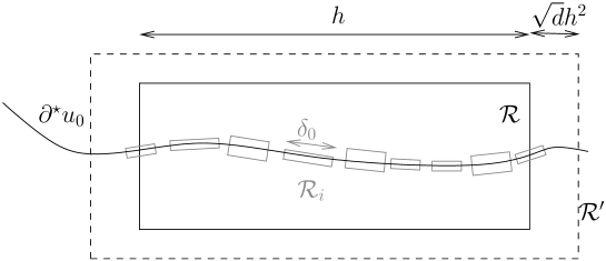
We will show that the right-hand side of (LABEL:eq-upb-pN) is negative, for small enough and . Thanks to (vi) in Definition 3.6, one sees (Figure 1) that the right-hand side of (LABEL:eq-upb-pN) is not larger, for and , than
where
is finite thanks to the definition of at (1.19). Now we give an upper bound on the integral. Since is convex, its slope is non-increasing and therefore
Now we show that . If not, we can extract a converging sequence in the compact set with as . The Fenchel-Legendre transform satisfies therefore
Since and are continuous (Proposition 2.5 in [Wou09]), we obtain in the limit , and therefore, by duality of the Fenchel-Legendre transform , which contradicts the assumption . The claim follows for any with . ∎
Proof.
(Proposition 3.12). Let . We take small enough so that we can use Lemma 3.13 with . Let and consider a -covering of . Proposition 3.11 in [Wou09] states that
for small enough. According to the definitions of and and to the properties of the coverings, provided was chosen small enough (still independently of ) we have
Finally when we take and large enough, Lemma 3.13 concludes the proof. ∎
Finally we remark that dilution has little influence on the overall magnetization
| (3.16) |
Proposition 3.14.
Assume that and . Let and . Let and consider a -covering of . Let and
the set of edges in some , or in some of the translates of by , for . Then, if is small enough,
Note that increases with every , therefore the condition that is the worse condition that one can consider.
Proof.
The proof is based on the renormalization procedure established in Theorem 5.10 in [Wou08]. As it is similar to that of Proposition 3.9 in [Wou09] we only sketch the argument. We cover with blocks with side-length . To these blocks is associated a family of independent random variables (independent of the ), the local -phase, that is zero with probability less than . Write and take some finite . A simple Peierls estimate shows that, given the condition , the -local phase associated to any block in is with a probability going to one as , uniformly in . As described in Theorem 5.10 in [Wou08], this event implies that
Therefore we just need to take small enough (named in Theorem 5.10 in [Wou08]) and small enough so that is negligible. ∎
3.3.3 The bottleneck
Here we focus on the bottleneck in the dynamics. We recall that the set , the set of sequences of profiles that evolve from to with jumps in -norm less than , was introduced at (1.23). Given , we call
Now, given , we define the -bottleneck set as
| (3.17) |
When are clear from the context, we simply write for . Note that our motivation for the above definition is that the -enlargement of is , a fact that helps in the proof of Lemma 3.17 below.
Now we state three Lemmas related to the bottleneck set. Lemma 3.15 gives the asymptotics of the probability that the phase profile belongs to . In Lemma 3.16 we show that is lower semi-continuous, a requisite for the proof of Lemma 3.17 in which we show how the gap in surface energy defined at (1.24) is related to the -enlargement of .
Lemma 3.15.
Assume and . Let and . There exists such that, for any -covering of with small enough, for any large enough,
Proof.
The exponential tightness property (Proposition 3.15 in [Wou09]) tells that there exists such that, for every , for any large enough,
(the set was defined at (3.13)). An immediate application of Markov’s inequality shows that
with a probability at least , for large . Since the surface cost of is bounded, we have therefore, for any , for any large enough, for large enough:
| (3.18) |
Now we take some and large. We take for the one given by Proposition 3.12 (it does not depend on ), and for any we denote by the parameter given by the same Proposition, and . Since the set is compact, it is covered with a finite number of balls
where , for all . Since the right-hand set is open while is compact, there is such that
and we can write
It follows then from Proposition 3.12 that, for any small enough, for any -covering of and any large enough,
| (3.21) |
Combining (3.21) with (3.18) proves the Lemma, provided that was chosen large enough. ∎
Lemma 3.16.
For any , the functional defined at (1.20) is lower semi-continuous.
Proof.
We show the lower semi-continuity as an application of the covering Proposition (Proposition 3.8). Let and , and consider a -covering for . Since the are disjoint, for any we have
since . Thanks to the lower semi-continuity of the surface energy in open sets (Chapter 14 in [Cer06]), the quantities and become not smaller than their value at when converges to in norm. Hence:
which is arbitrary close to for small , thanks to the uniform continuity of . ∎
Lemma 3.17.
For any ,
| (3.22) |
Proof.
We prove first that is larger or equal to the right-hand side. Let . Then,
and, when we optimize over and let we obtain the inequality
Now we prove the opposite inequality. Given any , there is such that
| (3.23) |
According to the definition of at (3.17), there is in , that is an -continuous evolution such that , , that satisfies
| (3.24) |
Now, for each we consider such that
| (3.25) |
We let also and . Clearly, the evolution is -continuous. Therefore, we have
The maximum in the right-hand side does not occur at since . We also have the bound
therefore,
where the second line is due to the definition of at (3.25), the third one to (3.24) and the last one to (3.23). The lower semi-continuity of (Lemma 3.16) imply that the last term goes to as . Therefore taking ends the proof. ∎
3.3.4 Intermediate formulation of the metastability
The aim of this Section is the proof of an intermediate and useful formulation of the metastability:
Proposition 3.18.
Assume and . Let , and small enough. Then, there exists such that, for any small enough, for any -covering of ,
where .
Important keys for the proof of Proposition 3.18 are Lemmas 3.15 and 3.17 about the bottleneck of the dynamics, together with Lemma 3.19 below on the so-to-say “continuous evolution” of the magnetization profile.
Lemma 3.19.
Let and . There is such that, for any large enough,
where is a uniform upper bound on the rates of the Glauber dynamics.
Proof.
(Lemma 3.19). The distance is bounded by times the number of jumps of the Glauber dynamics. These jumps occur at a rate bounded by . Therefore,
where is a Poisson variable with parameter . Cramér’s Theorem imply the claim. ∎
Proof.
(Proposition 3.18). In view of Proposition 3.11 it suffices to prove that
| (3.26) |
where
So we focus on the proof of (3.26). We remark that, for any initial configuration ,
since and , for any . Therefore
| (3.30) | |||||
| (3.33) |
where the second inequality is a consequence of Markov’s inequality. Now we fix and and call
the event of continuity, and
the event that the magnetization profile is close to at any time . Then we remark that
| (3.39) |
Indeed, the definition of yields a sequence . We can take since we know that . This sequence is -continuous according to the properties of the and to the definition of . Finally, we have
| (3.40) | |||||
and therefore . So we can fix , which makes the evolution -continuous.
Now we conclude the proof of (3.26). As a consequence of (3.33) and (3.39) we have the inequality
and therefore, according to the invariance of for the Glauber dynamics, and to the definition (3.17) of the bottleneck set ,
where
Finally we bound each contribution separately. First, according to Lemmas 3.15 and 3.17 we have
for small enough, for some , and for any -covering of with small enough, for any large enough. So for
we have, under the same conditions,
| (3.42) |
Then, the exponential tightness property (see (3.18) above) implies that, for large enough,
| (3.43) |
and finally Lemma 3.19 implies that, for large , uniformly over and ,
| (3.44) |
Summing the last three displays yields (3.26). ∎
3.3.5 Proofs of Theorems 2.2 and 2.5
Here we conclude the proof of Theorems 2.2 and 2.5. We state one more Lemma that relates the averaged autocorrelation defined at (1.8) to the dynamics of the overall magnetization defined at (3.16).
Lemma 3.20.
For any , and one has
| (3.45) |
Proof.
Minkowski’s inequality implies, for any , that
where is the function which associates, to the spin configuration , the spin at , . Taking , the translation invariance of and of the Glauber dynamics implies that
Hence, for any we have
and we conclude by using the attractivity of the Glauber dynamics:
| (3.46) | |||||
∎
Proof.
(Theorem 2.2). Let and . We assume that , otherwise there is nothing to prove. We fix and such that
Then, for any we call the smallest integer such that . According to Lemma 3.20, to Propositions 3.14 and 3.18, to Lemma 3.10, for any small enough we can find such that, provided that is large enough,
The definition of implies finally that
for large enough, and this gives the claim as . ∎
Proof.
(Theorem 2.5) Let and assume that . There exists and such that
Given large, we define an intermediate side-length as the largest integer such that
First, we prove that the event of dilution, on scale , occurs with large probability inside . More precisely, we consider and
We also consider and a -covering for , and for any we call
the -translate of . According to Lemma 3.10 we have, for small enough,
| (3.47) | |||||
where we use the definition of and the fact that , for some . We call now the event that is the smallest box for which dilution occurs, where is ordered according to the lexicographic order. According to Proposition 3.18 and to the attractivity of the dynamics, the conditional probability
goes to as (and thus ). On the other hand, Proposition 3.14 and the monotonicity of the system imply that, as well, the conditional probability
goes to as . Therefore, we have shown that the -probability that there exists with both
goes to one as . Taking as a test function in (1.30) proves the lower bound on the relaxation time. For obtaining the lower bound on the mixing time one can consider in (1.32), and any initial configuration for which , which is possible as this event has positive probability. ∎
3.4 The geometry of relaxation
The first part of this Section is dedicated to the proof of Proposition 2.1. Then we show that the gap in surface energy can be computed on more restrictive evolutions, and finally we compute for two simple initial configurations.
3.4.1 A lower bound on the gap in surface energy
The statement of theorems 2.2 and 2.5 is non-empty only if happens to be strictly positive for some initial profiles . We state the next Theorem, which has Proposition 2.1 as a Corollary:
Theorem 3.21.
Let . Assume that the boundary of is . There exists a non-decreasing function , with , , that depends only on , such that
| (3.48) |
Proof.
(Proposition 2.1). When for all and the boundary of is , it follows at once from (3.48) that . Now we address the proof of (2.2). We discuss first the consequences of the assumption . When along a section of a rectangle the surface tension in that rectangle is , thus for all , all ,
| (3.49) |
Now we consider the initial configuration defined by
where . According to (3.49) there is not depending on such that the cost of dilution defined at (1.22) satisfies . We also have where is the initial surface energy defined at (1.20), and is the perimeter of . So we conclude already that the numerator in the definition (2.1) of is bounded by a constant which does not depend on . Finally we recall that, thanks to the assumption that and to Proposition 2.13 in [Wou09],
| (3.50) |
and therefore the inequality (3.48) implies that, for some and for all large enough,
The convexity and the lattice symmetries of the Wulff crystal imply that the ratio
is bounded from below by some constant not depending on , hence
for large . The claim (2.2) follows. ∎
The proof of Theorem 3.21 requires three Lemmas, that are stated now together with their proof. We introduce the new surface energy
| (3.51) |
Lemma 3.22.
Let and . Then, the profiles and satisfy
| (3.52) |
Proof.
We remark first that
| (3.53) |
As stated in Theorem 3.61 in [AFP00], given any the local density of at is either or , for -almost all , and the set of points at which the local density is coincides, up to a -negligible set, to the reduced boundary (denoted in [AFP00]). This implies the two equalities
| (3.54) | |||||
| (3.55) |
up to -negligible sets, where stands for the disjoint union (again, up to -negligible sets). Furthermore, the outer normal at (resp. ) corresponds (-a.s.) to the outer normal at (resp. to the opposite of the former). Thus, in conjunction with (3.53), equations (3.54) and (3.55) imply respectively the and the part of (3.52). ∎
Lemma 3.23.
Let and . For any , there is a finite collection of droplets such that
-
i.
The are disjoint and their union is ,
-
ii.
Each is included in a box of side-length at most ,
-
iii.
And
(3.56)
Proof.
Lemma 3.24.
Assume that , and satisfy
| (3.57) |
for all , where . Then
| (3.58) |
where is a constant that depends only on .
Proof.
We let
The surface tension associated to is
and it satisfies obviously the relations
therefore
| (3.59) |
The isoperimetric inequality for (see [KP94]) implies in turn that
| (3.60) |
so the claim will follows from an appropriate lower bound on the volume . There exists such that . Now we take , close to , and prove that it lies in : if , then
as the Euclidean norm of is not larger than . According to our assumption (3.57) it follows that
The set is convex and contains all the images of by the symmetries of , therefore it contains an hypercube which vertices are the images of by the above mentioned symmetries. Consequently the volume of is at least of the volume of the ball and the proof is over. ∎
Proof.
(Theorem 3.21). Given , the continuity of and the smoothness of imply that there exists such that
As we claimed, depends only on , and of course on . Also, it is clear that one can chose the function non-decreasing. Furthermore, to a given direction corresponds such that and therefore
It follows that any with diameter not greater than satisfies assumption (3.57) of Lemma 3.24 when one takes
Now we consider some phase profile , call and the profiles given by Lemma 3.22, and then the union of the droplets associated to both and by Lemma 3.23. In conjunction with Lemma 3.24, we obtain
According to the definition of and of the we have
therefore, the trivial inequality for and implies that, for every ,
But is maximized for and equals . So, taking , for any at -distance from (this distance is smaller than the distance between and if we require that be small), we get
and we have proved (3.48) with , as . ∎
3.4.2 Continuous evolution and continuous separation
In this paragraph we give an alternative formulation of the surface energy gap . We introduce a set of continuous evolution of the phase profile, for which the boundary splits continuously from its original location:
| (3.62) |
and then define , the gap in the free energy associated to the optimal droplet removal in this class of evolutions:
| (3.63) |
Theorem 3.25.
For all ,
The inequality is clear since the set is more restrictive that those evolutions considered in the definition (1.24) of . We prove the reverse inequality with the help of an interpolation: given an evolution (see (1.23)) we interpolate from a continuous evolution with continuous separation from , at the price of a small increase in the maximal cost, negligible as (and uniform over ):
The next lemma is one of the keys to the proof of Theorem 3.25.
Lemma 3.26.
Let and . For any Borel set with volume , there exists a collection of measurable sets such that:
-
i.
is a non-decreasing function with
where is the tube .
-
ii.
The function is -periodic.
-
iii.
The volume is a continuous function of
-
iv.
The area is a continuous function of
-
v.
The portion of the boundary of that intersects in has a small area:
for small enough.
Proof.
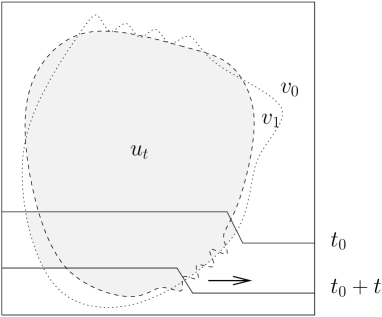
See Figure 2 for an illustration of the proof. To begin with, we partition in horizontal slabs: let and call
for . Because each slab has a volume at least , for each there exists such that the density of at height is not larger than . We extend then the definition of by periodicity, letting
Then, we let for some such that has no face orthogonal to and define
where is the piecewise linear function defined by: ,
and linear on each interval . The set evolves as follows: between times and , invades the region by the mean of a front line normal to , that moves at a constant speed.
It is immediate from the definition that is -periodic and that increases continuously in volume. The measure of is non-decreasing and the assumption on ensures that it increases continuously. We consider at last the portion of the surface of in that might intersect . We just have to take into account the upper portion of , made of the two planes at height , and of a portion of plane normal to . Recall that the have been chosen so that the density of at height does not exceed . Similarly, because , the piece of plane orthogonal to has a surface at most for small enough. The claim follows. ∎

The second key argument is periodicity: as seen on Figure 2, the interpolation between and has to choose first the region where the cost of is smaller than that of – which means that we have to fix carefully.
Proof.
(Theorem 3.25). Let . There exists and , together with , such that
Starting from , we construct a continuous evolution that has a maximal cost not much larger than that of . It is enough to do the interpolation between two successive , as one can paste together the successive interpolations to deduce the continuous evolution .
Hence we consider and assume that . We let
which has a volume at most . Lemma 3.26 applies and there is with properties (i)-(v). Given and we let
for any the set increases continuously from the empty to the full set in , makes the surface a continuous function of , and the area
small, for small enough. Now we define
The cost of decomposes in the following way: it is the sum of the cost of in , of the cost of in , and of the cost of in . In other words,
| (3.64) |
where stands for
It is clear that the initial cost of is and that its final cost is . Yet in the interval it could be that selects first the region where has a larger cost than , leading to a maximal cost larger than expected. We rule out this possibility with an appropriate choice for – see Figure 2 for an illustration of the discussion below.
For and we consider
Our aim is to extend to arbitrary values of . For , we denote by the translated of by , then for any and we have
from the definition of . The latter formula permits to extend to and puts in evidence the existence of a function such that
This function is, apart from a linear correction, -periodic: for all ,
in other words,
where is a -periodic function. Now we fix such that
it is immediate that
Reporting into (3.64) we conclude that is a satisfactory interpolation between and : provided that is small enough,
∎
3.4.3 The gap in surface energy in the isotropic case
In this paragraph we use Theorem 3.25 to compute the gap in surface energy in the two dimensional, isotropic case.
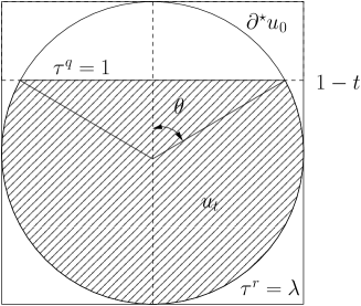
Lemma 3.27.
Assume , for all and consider
where is the disk of radius centered at , and . Then
An optimal continuous evolution in this setting is illustrated on Figure 3.
Proof.
In order to simplify the notation we will consider . The upper bound
is immediate if one considers the continuous evolution defined by
and satisfying , as illustrated on Figure 3. The lower bound is scarcely more difficult to establish: given a continuous evolution with continuous detachment, there is such that

Optimizing the droplets of as in Figure 4 – we replace each portion of the interface not in with a segment (step (1)) – we obtain a profile with a lower cost, yet it still has the same contact length with . By isotropy of surface tension it is possible to aggregate the droplets together (step (2)) and obtain with a unique droplet and a lower cost, preserving again the length of contact. At last, inverting the order of the segments and arcs and optimizing again we see that the profile of lower cost that satisfies coincides, apart from a rotation, with the profiles considered in the upper bound. The claim follows. ∎
3.4.4 The gap in surface energy when the Wulff crystal is a square
Here we compute the gap in surface energy for another simple case, when the Wulff crystal is a square. We also show that the gap in surface energy is strictly bigger than the cost of the less likely overall magnetization.
Lemma 3.28.
Assume , for all and
where , and . Then, we have
Proof.
Again we consider in order to simplify the notations. The upper bound on the additional cost is immediate considering . For the lower bound we need a finer analysis. First, it is a consequence of the assumption on that for any open, connected with extension in the canonical directions, that is:
we have
Then, we decompose a profile configuration into its droplets . We call the extension of in the canonical directions and let the length of contact between and , so that, for all :
If a droplet touches two opposite faces of , say , then its extension in the orthogonal direction is at least and the inequality
follows. If on the opposite the droplet is in contact with at most two adjacent sides of , we have and hence
Assume now that the total length of contact is , i.e. that . A consequence of the former lower bounds is that, whether or not some droplet touches two opposite faces, the cost of is at least . The claim follows. ∎
We conclude this work with a comparison between the bottleneck due to the positivity of and the one due to the continuous evolution of the magnetization:
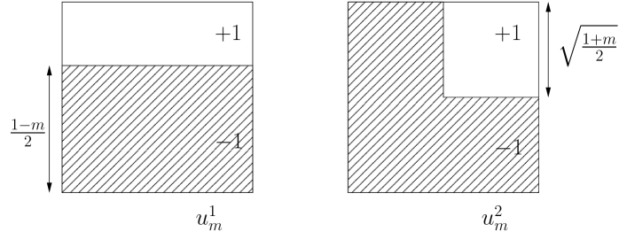
Lemma 3.29.
In the settings of the former lemma, with furthermore , we have
Proof.
We provide an upper bound for the right hand term, considering for a given the two profiles (see Figure 5)
and
that both satisfy the volume constraint . It is immediate that
hence
Note that decreases with while increases with . Because of their extremal values there exists some at which , and since we have in particular which is the maximal cost of an optimal continuous detachment evolution. ∎
Acknowledgements. It is a pleasure to thank Thierry Bodineau for his commitment and continuous support throughout the duration of this work. I am also grateful to Fabio Martinelli for pointing out the scheme of proof of Theorem 2.4.
References
- [ACCN87] M. Aizenman, J. T. Chayes, L. Chayes, and C. M. Newman. The phase boundary in dilute and random Ising and Potts ferromagnets. J. Phys. A, 20(5):L313–L318, 1987.
- [ACCN88] M. Aizenman, J. T. Chayes, L. Chayes, and C. M. Newman. Discontinuity of the magnetization in one-dimensional Ising and Potts models. J. Statist. Phys., 50(1-2):1–40, 1988.
- [AFP00] L. Ambrosio, N. Fusco, and D. Pallara. Functions of bounded variation and free discontinuity problems. Oxford Mathematical Monographs. The Clarendon Press Oxford University Press, New York, 2000.
- [BGW12] T. Bodineau, B. Graham, and M. Wouts. Metastability in the dilute Ising model. Probab. Theory Related Fields, to appear.
- [BI04] T. Bodineau and D. Ioffe. Stability of interfaces and stochastic dynamics in the regime of partial wetting. Ann. Henri Poincaré, 5:871–914, 2004.
- [BM02] T. Bodineau and F. Martinelli. Some new results on the kinetic Ising model in a pure phase. J. Statist. Phys., 109(1-2):207–235, 2002.
- [Cer06] R. Cerf. The Wulff crystal in Ising and percolation models, volume 1878 of Lecture Notes in Mathematics. Springer-Verlag, Berlin, 2006.
- [CMST10] P. Caputo, F. Martinelli, F. Simenhaus, and F. L. Toninelli. “Zero” temperature stochastic 3D Ising model and dimer covering fluctuations: a first step towards interface mean curvature motion. http://arxiv.org/abs/1007.3599, 2010.
- [ES88] R. G. Edwards and A. D. Sokal. Generalization of the Fortuin-Kasteleyn-Swendsen-Wang representation and Monte Carlo algorithm. Phys. Rev. D (3), 38(6):2009–2012, 1988.
- [Fed69] H. Federer. Geometric measure theory. Die Grundlehren der mathematischen Wissenschaften, Band 153. Springer-Verlag, New York, 1969.
- [HF87] D. A. Huse and D. S. Fisher. Dynamics of droplet fluctuations in pure and random Ising systems. Phys. Rev. B, 35(13):6841–6846, 1987.
- [KP94] R. Kotecký and C.-E. Pfister. Equilibrium shapes of crystals attached to walls. J. Statist. Phys., 76(1-2):419–445, 1994.
- [LMST10] E. Lubetzky, F. Martinelli, Allan Sly, and Fabio Lucio Toninelli. Quasi-polynomial mixing of the 2D stochastic Ising model with “plus” boundary up to criticality. http://arxiv.org/abs/1012.1271, 2010.
- [LS10] E. Lubetzky and A. Sly. Critical ising on the square lattice mixes in polynomial time. http://arxiv.org/abs/1001.1613, 2010.
- [Mar99] F. Martinelli. Lectures on Glauber dynamics for discrete spin models. In Lectures on probability theory and statistics (Saint-Flour, 1997), volume 1717 of Lecture Notes in Math., pages 93–191. Springer, Berlin, 1999.
- [MT10] F. Martinelli and F. L. Toninelli. On the mixing time of the 2D stochastic Ising model with “plus” boundary conditions at low temperature. Comm. Math. Phys., 296(1):175–213, 2010.
- [Sch94] R. H. Schonmann. Slow droplet-driven relaxation of stochastic Ising models in the vicinity of the phase coexistence region. Comm. Math. Phys., 161(1):1–49, 1994.
- [SS98] R. H. Schonmann and S. B. Shlosman. Wulff droplets and the metastable relaxation of kinetic Ising models. Comm. Math. Phys., 194(2):389–462, 1998.
- [Tho89] L. Thomas. Bounds on the mass gap for the finite volume stochastic Ising models at low temperatures. Comm. Math. Phys., 126(1):1–11, 1989.
- [Wou07] M. Wouts. The dilute Ising model: phase coexistence at equilibrium & dynamics in the region of phase transition. PhD thesis, Université Paris 7 - Paris Diderot, http://tel.archives-ouvertes.fr/tel-00272899, 2007.
- [Wou08] M. Wouts. A coarse graining for the Fortuin-Kasteleyn measure in random media. Stochastic Process. Appl., 118(11):1929–1972, 2008.
- [Wou09] M. Wouts. Surface tension in the dilute Ising model. The Wulff construction. Comm. Math. Phys., 289(1):157–204, 2009.