The cost of continuity: performance of iterative solvers on isogeometric finite elements

Abstract

In this paper we study how the use of a more continuous set of basis functions affects the cost of solving systems of linear equations resulting from a discretized Galerkin weak form. Specifically, we compare performance of linear solvers when discretizing using $C^{0}$ B-splines, which span traditional finite element spaces, and $C^{p-1}$ B-splines, which represent maximum continuity. We provide theoretical estimates for the increase in cost of the matrix-vector product as well as for the construction and application of black-box preconditioners. We accompany these estimates with numerical results and study their sensitivity to various grid parameters such as element size $h$ and polynomial order of approximation $p$. Finally, we present timing results for a range of preconditioning options for the Laplace problem. We conclude that the matrix-vector product operation is at most $\left.33p^{2}\middle/8\right.$ times more expensive for the more continuous space, although for moderately low $p$, this number is significantly reduced. Moreover, if static condensation is not employed, this number further reduces to at most a value of 8, even for high $p$. Preconditioning options can be up to $p^{3}$ times more expensive to setup, although this difference significantly decreases for some popular preconditioners such as Incomplete LU factorization.

1 Introduction

Isogeometric analysis (IGA) [15, 7] is a Galerkin finite element method which has popularized the use of the Non-uniform Rational B-spline (NURBS) basis for solving partial differential equations (PDE’s). The computer aided design (CAD) community has long used NURBS as a basis due to its higher-order continuity, ideal for designing smooth curves and surfaces. The higher order continuous basis also enables the use of the standard Galerkin method for solving higher order problems [13, 14, 10]. Furthermore, it has been observed that the approximability of the higher continuous spaces per degree of freedom is superior to that of traditional finite element spaces for problems with smooth solutions. This suggests that IGA not only links geometry to analysis but also is an efficient method for solving a variety of PDE’s.

As for any Galerkin method, the main computational cost of IGA comes from the assembly and solution of a system of linear equations. When using a direct method to solve this linear system, we showed in [6] that for large three dimensional problems of given polynomial order $p$, the number of floating point operations (FLOPS) needed to solve a $C^{p-1}$ discretization is approximately $p^{3}$ times more expensive than that of a $C^{0}$ discretization with the same order of approximation $p$ and same number of degrees of freedom (DOF). In other words, each DOF is $p^{3}$ times more expensive to solve when using $C^{p-1}$ discretizations as opposed to using $C^{0}$ discretizations. This theoretical estimate was corroborated by our numerical experiments for problem sizes of practical interest.

In this work, we extend our previous study to the case of iterative solvers. The main motivation for using iterative methods is to reduce computational cost (time and memory). However, in general there are no a priori estimates for the computational time required by the iterative solver because it is a composition of many factors. These costs include matrix-vector multiplications and additional operations required by the iterative method (vector scalings, dot products) as well as the cost of setting up and applying the preconditioner. While these costs may be estimated, their influence on the overall computational time tightly depends on the number of iterations required to reduce the linear algebra error to a prescribed tolerance. For example, it often occurs that a preconditioner which leads to few required iterations for convergence is also more expensive to construct and/or apply. In the limit, a LU factorization is the ideal preconditioner in terms of iteration count, however is expensive to construct and apply.

To develop a baseline understanding for how continuity affects iterative solvers, we study the canonical Laplace problem discretized using $C^{0}$ and $C^{p-1}$ B-spline spaces, representing minimum and maximum continuity. We only consider the matrix-vector multiplication component of the iterative solver. The additional operations required by different iterative methods (vector updates, orthogonalizations) are not dependent on the basis used, and therefore may be ignored when comparing how continuity affects the iterative solver. To better expose the effect of continuity on the cost of the solver, we use preconditioned conjugate gradients (CG) as our iterative method, because it is among the most efficient methods in the Krylov family [21, 22].

We will study a range of standard preconditioners which are appropriate for small and medium size problems. These include: diagonal Jacobi, successive overrelaxation, incomplete LU factorization, and element by element. Despite the fact these methods do not scale to large problems, they are frequently used as building blocks to construct more complex preconditioners (approximate solvers on subdomains of domain decomposition and physics-based preconditioners or smoothers in multigrid techniques [20, 1, 2]). Most of the techniques we will study here are described in Saad’s book [21] and implemented in scientific software frameworks such as PETSc [5, 4]. It is our aim to assess the additional cost incurred by a more continuous basis as well as illuminate how standard approaches work for IGA discretizations.

This study complements the only previous published work on iterative solvers for IGA discretizations of which we are aware. In [8] Beirão da Veiga, et. al. propose a large family of domain-decomposition two-grid solvers and prove theoretically that the condition number of the preconditioned system is independent of element size $h$. They also provide numerical evidence showing that the condition number is independent of $p$ provided that the overlap between subdomains is sufficiently large. However, these numerical results are concerned only with convergence (condition number and number of iterations) and not with computational efficiency.

The rest of this paper develops in the following manner. In section 2 we detail the model problem used throughout this work. Section 3 derives theoretical estimates of FLOPS needed to perform matrix-vector multiplications of linear systems resulting from $C^{0}$ and $C^{p-1}$ discretizations, as well as estimates for the setup and application of different preconditioners. In section 4 we present numerical results to complement the theory. We show convergence in terms of iterations as well as computational time on a range of discretizations varying in $h$ and $p$.

2 Model Problem

The problem used for our study is the Laplace equation in three dimensions on the unit cube,

$$-\nabla\cdot(\nabla u) =0\ \ \ \text{on }\Omega$$ (1)

$$u =1\ \ \ \text{on }\Gamma_{D}$$

$$(\nabla u)\cdot\mathbf{n} =0\ \ \ \text{on }\Gamma_{N}$$

where $\Omega=[0,1]^{3}$, $\Gamma_{D}=(0,:,:)\cup(:,0,:)\cup(:,:,0)$, and $\Gamma_{N}=(1,:,:)\cup(:,1,:)\cup(:,:,1)$. We will use uniform $h$-refinements of $C^{0}$ and $C^{p-1}$ B-splines to discretize the weak form of the Laplace equation.

3 Theory

In this section we develop theoretical estimates for the increase in cost associated with the use of higher continuous spaces in Galerkin finite elements. We assess cost by counting the FLOPS required by matrix-vector products and the setup of different preconditioning options. We use these estimates as a measure of the relative cost between $C^{0}$ and $C^{p-1}$ spaces.

3.1 Matrix-Vector Multiplication

The main cost of iterative methods is due to the matrix-vector multiplication operation which is proportional to the number of nonzero entries in both the system and preconditioner matrix. We develop estimates for the number of nonzero entries in the stiffness matrix of the model problem resulting from $C^{0}$ and $C^{p-1}$ discretizations in three spatial dimensions. We do this by considering the number of nonzero entries that a single element of a structured grid mesh contributes to the system matrix.

We begin by considering a single element of a 1D, $C^{0}$ discretization of order $p$. Consider figure 1 where we have drawn such an element, particularized to a cubic for the sake of illustration. The number of nonzero entries to the matrix will be the sum of the interactions that each basis has with all other basis functions which have overlapping support. We note that in the 1D case, there are two classes of interactions–those associated to the vertices and the interior of the element. We note that a basis associated to a vertex overlaps $2p+1$ others while the bases associated to interiors overlap $p+1$ others. We consider a DOF for a single vertex per element (since the other vertex is actually the first vertex of the next element) and $p-1$ DOFs per interior. The total number of nonzero entries accumulated due to a single element is then $(1)(2p+1)+(p-1)(p+1)$. This number is attained by summing over all entities the total number of interactions of all the DOFs associated to that entity.

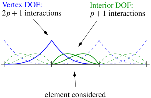
Fig. 1: Sample cubic $C^{0}$ discretization with a single element highlighted.

For the multidimensional case, we extend this method of counting the nonzero entries of the matrix by a tensor product construction. In addition to vertex and interior DOFs, we have DOFs associated to edges in two and three dimensions as well as DOFs associated to faces in three dimensions. We summarize the enumeration of DOFs and their interactions in table 1. The total number of nonzeros due to a single element contribution is the row sum of the product of all columns in this table. Specially, for three dimensions we have

$$\mbox{nnz}^{C^{0}}$$

(2)

Table 1: Summary table of the interactions of degrees of freedom associated with a $C^{0}$ basis.

		Number	DOFs	Number
Dimension	Entity	of Entities	per Entity	of interactions
1D	vertex	1	1	$(2p+1)$
1D	interior	1	$(p-1)$	$(p+1)$
2D	vertex	1	1	$(2p+1)^{2}$
2D	edge	2	$(p-1)$	$(2p+1)(p+1)$
2D	interior	1	$(p-1)^{2}$	$(p+1)^{2}$
3D	vertex	1	1	$(2p+1)^{3}$
3D	edge	3	$(p-1)$	$(2p+1)^{2}(p+1)$
3D	face	3	$(p-1)^{2}$	$(2p+1)(p+1)^{2}$
3D	interior	1	$(p-1)^{3}$	$(p+1)^{3}$

In the case of $C^{p-1}$ B-splines, the interactions are more regular because each basis interacts with $(2p+1)^{3}$ others. To make the estimates comparable, in terms of unknowns, to the single element of $C^{0}$ basis functions, we multiply by $p^{3}$.

$$\mbox{nnz}^{C^{p-1}}=p^{3}(2p+1)^{3}=8p^{6}+12p^{5}+6p^{4}+p^{3}={\cal O}(8p^{6})$$ (3)

We conclude that in the case of large $p$ the increase in cost of matrix vector multiplication of $C^{p-1}$ spaces is no more than eight times that of $C^{0}$ spaces. However, for the range of meaningful discretizations of polynomial order $p$, we see this factor smaller than the limit, approximately two for $p=2$ and three for $p=3$. In table 2 we present some numerical results for the actual ratios of times for 1000 matrix-vector products of $C^{p-1}$ and $C^{0}$ spaces as the number of degrees of freedom, $N$, in the system increases. We compare these time ratios to the theoretical ratio of number of nonzero entries for a system of infinite size, equation (3) divided by equation (2).

Table 2: Actual and estimated increase in cost of a matrix-vector multiply for $C^{p-1}$ spaces relative to $C^{0}$ spaces.

	Polynomial order, $p$
$N$	$2$	$3$	$4$	$5$
$10^{3}$	1.19	1.95	1.93	0.94
$10^{4}$	1.76	2.22	2.96	3.19
$10^{5}$	1.74	2.56	3.02	3.46
$10^{6}$	1.80	2.60	3.08	3.51
$\infty$	1.95	2.74	3.37	3.88

Note on Static Condensation

When using $C^{0}$ spaces, it is common to first eliminate (using Gaussian elimination) all DOF interior to an element, a technique known as static condensation [26]. This approach is also used in a multi-frontal direct solver algorithm [11, 12] and known to be of reduced value when using $C^{p-1}$ spaces (see [6]). Iterative solvers can also make use of the technique, solving on the reduced system, called the skeleton problem. The skeleton problem is not only of smaller rank than the original, but it also contains fewer nonzero entries. This affects the iterative solver in that the matrix-vector multiplications are economized.

To see this effect, we compute the number of nonzeros for a single element in the resulting matrix after performing static condensation. We repeat a portion of table 1 which corresponds to the three dimensional results in table 3. If we statically condense the interior DOFs, these nonzero entries are now removed (the row of the table is removed). However, we also need to remove all interactions that the vertices, edges, and faces have with interior DOFs. To this end, we have added another column which represents these DOFs. For each entity we eliminate $(p-1)^{3}$ DOFs which correspond to each interior to which that entity was connected. Vertices connect to eight interiors, edges to four interiors, and faces to two interiors. We then sum the nonzero entries as before.

Table 3: Summary table of the interactions of degrees of freedom associated with a $C^{0}$ basis in three dimensions with the interior DOFs statically condensed.

	Number	DOFs	Number	Statically
Entity	of Entities	per Entity	of interactions	condensed
vertex	1	1	$(2p+1)^{3}$	$-8(p-1)^{3}$
edge	3	$(p-1)$	$(2p+1)^{2}(p+1)$	$-4(p-1)^{3}$
face	3	$(p-1)^{2}$	$(2p+1)(p+1)^{2}$	$-2(p-1)^{3}$

$$\mbox{nnz}_{sc}^{C^{0}}$$

(4)

For large enough problems, the matrix-vector product of $C^{0}$ spaces becomes $\left.p^{2}\middle/33\right.$ more expensive that the statically condensed system. In the case of $C^{p-1}$ spaces, this number approaches $\left.8p^{2}\middle/33\right.$. While the process of static condensation incurs additional cost in the matrix assembly phase, in practice this approach is more efficient than standard $C^{0}$ approaches and not worthwhile in the case of $C^{p-1}$ spaces. See table 4 for comparison of theory to timing results.

Table 4: Actual and estimated increase in cost of a matrix-vector multiply for $C^{p-1}$ spaces relative to $C^{0}$ spaces with static condensation.

	Polynomial order, $p$
$N$	$2$	$3$	$4$	$5$
$10^{3}$	1.32	2.66	3.26	2.00
$10^{4}$	1.96	3.07	5.14	6.87
$10^{5}$	1.95	3.56	5.29	7.58
$10^{6}$	2.00	3.62	5.42	7.74
$\infty$	2.16	3.81	5.93	8.54

While the gains in static condensation when using relatively low $p$ are moderate, for higher $p$ the added efficiency is of greater importance. In figure 2 we plot the theoretical ratios of the number of nonzero entries for $C^{p-1}$ relative to $C^{0}$ spaces with and without static condensation. These plots represent, as $p$ increases, how much more expensive a matrix-vector product is when using $C^{p-1}$ spaces. When no static condensation is used, we see that the increase asymptotically approaches (slowly) a factor of eight. However, when compared to the use of static condensation, the increase in cost continues to grow with high $p$. If one is to advocate the use of $C^{p-1}$ basis functions as a high $p$ method, the merits of the basis must be weighed against this increase in cost.

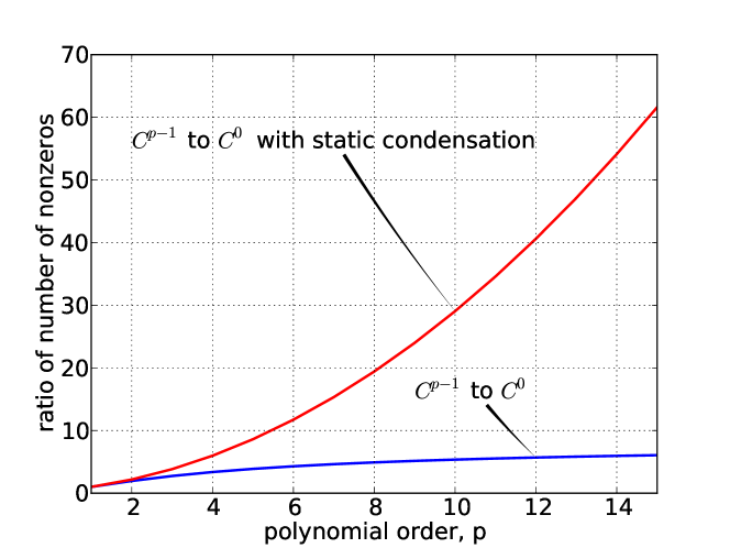
Fig. 2: The theoretical ratio of the number of nonzeros in system matrices, independent of the number of unknowns.

3.2 Black-box Preconditioners

Now we consider how more continuous bases affect black-box preconditioning techniques, such as those found in [21] (Chapter 10, pages 317–339). We develop theoretical cost estimates in terms of FLOPS for both forming and applying each preconditioner. In the paragraphs to follow we briefly describe each preconditioner and explain how these estimates may be formed.

Diagonal Jacobi

Practical implementations of diagonal Jacobi preconditioning extract the diagonal entries from the matrix and invert them, storing the result in a vector. The application of the preconditioner is then performed by point-wise multiplication of residual entries with the diagonal inverses. Both the setup and application of this preconditioner require $N$ FLOPS, independent of the continuity of the basis.

Symmetric Successive Overrelaxation (SSOR)

The SSOR preconditioner is based on a relaxation scheme, similar to Gauss-Seidel iterations. Practical implementations of SSOR preconditioning extract the diagonal entries from the matrix, invert, and scale them by the relaxation parameter in order to make the application of the preconditioner more economical. The application of this preconditioner consists of forward and backward sweeps, which roughly amounts to a single matrix-vector product.

Incomplete LU factorization (ILU)

Incomplete LU factorization (ILU) is a preconditioning technique based on Gaussian elimination. Here we address only ILU with zero fill-in. The ILU preconditioner is formed by performing LU factorization, omitting entries which would change the nonzero pattern of the original matrix. Thus, ILU is a crude approximation to the LU factors of the system matrix, however more economical to compute and apply.

Implementations of the zero fill-in ILU preconditioner are based in the $IKJ$ (see the discussion in [21] starting on page 304) version of Gaussian elimination on the static non-zero pattern of the input sparse matrix. The algorithm traverses the sparse matrix by rows. At each row, the Gaussian elimination algorithm is applied on only the nonzero entries.

Denoting $L_{i}$ the number of nonzero entries in the strictly lower-triangular part of the $i$-th row and $U_{k}$ the number of nonzero entries in the strictly upper-triangular part of the $k$-th row, the number of FLOPs required to eliminate the $i$-th row is $L_{i}(1+2U_{k})$.

For a $C^{p-1}$ system matrix, every row has $(2p+1)^{3}$ nonzero entries, thus the the number of nonzero entries in the strictly lower-triangular and upper-triangular parts of $i$-th and $k$-th rows are

$$L_{i}=U_{k}=\frac{(2p+1)^{3}-1}{2}$$

and the total number of FLOPS for $N$ rows is

$$\text{FLOPS}^{C^{p-1}}_{\text{ILU}}=N\left(32p^{6}+96p^{5}+120p^{4}+76p^{3}+24p^{2}+3p\right)$$

For a $C^{0}$ system matrix, the number of nonzeros per row depends on the kind of DOF (see previous subsection) and obtaining analytic estimates is much more involved. We use instead a computational approach consisting on building the graph for a mesh of $5\times 5\times 5$ elements for a $C^{0}$ discretization of degree $p=1\ldots 7$. For every $p$, we compute the preconditioner row-by-row and add-up the number of FLOPS required for performing the ILU factorization for the middle element. By using polynomial fitting, we obtain the coefficients of a degree 6 polynomial. Finally, the cost of constructing the ILU preconditioner for a $C^{0}$ system matrix is

$$\text{FLOPS}^{C^{0}}_{\text{ILU}}=N\left(\frac{2}{3}p^{6}+\frac{26}{3}p^{5}+\frac{128}{3}p^{4}+\frac{601}{6}p^{3}+\frac{355}{3}p^{2}+\frac{200}{3}p+\frac{83}{6}\right)$$

We highlight that the ILU preconditioner is inexpensive relative to the full LU factorization and is in both cases of order $N$. We also note that in three spatial dimensions, the highest order term in terms of the polynomial order is $p^{6}$ for both $C^{0}$ and $C^{p-1}$ spaces. In the case of large $p$ the increase in cost of matrix vector multiplication of $C^{p-1}$ spaces is no more than 48 times that of $C^{0}$ spaces. In the summary table 5, we only include these leading terms in order to more succinctly compare preconditioners. The application of this preconditioner consists of forward and backward substitution steps, which roughly amounts to a single matrix-vector product.

Element-by-element (EBE)

In the context of $C^{0}$ finite element spaces, an additive-Schwarz [23] preconditioner may be constructed in the limit where the subdomains are the elements of the finite element discretization. This preconditioner is known as the element-by-element preconditioner (EBE). Note that this preconditioner departs from that described in [21] and follows [20]. Given the fully assembled system matrix, this preconditioner is constructed by extracting the local element matrix and inverting it explicitly. The inverse of the local element matrix is assembled into a preconditioner matrix which has the same nonzero pattern as the original system matrix.

The cost of constructing the preconditioner for both $C^{0}$ and $C^{p-1}$ spaces is the number of elements, $N_{e}$, times the cost of inverting the small blocks,

$$N_{e}\left(2p^{9}\right)$$

We note that for $C^{0}$ discretizations the number of degrees of freedom $N$ can be related to the number of elements by the relationship, $N=\mathcal{O}(N_{e}p^{3})$. Therefore, the preconditioner cost can then be expressed in terms of number of degrees of freedom as, $2Np^{6}$. In $C^{p-1}$ spaces, the number of elements is roughly the number of degrees of freedom, $N=\mathcal{O}(N_{e})$ which leads to the total cost being $2Np^{9}$. We emphasize that in this case, the resulting matrix-vector product is no more expensive than for the original system matrix. This means that the EBE preconditioner is again at most 8 times more expensive to apply for $C^{p-1}$ spaces when compared to $C^{0}$.

Basis by Basis (BBB)

For $C^{p-1}$ spaces, we also construct an additive-Schwarz type preconditioner based on the family of preconditioners presented in [8]. We consider a selection of these preconditioners constructed by taking single basis function subsets of the function space. We explore the performance of this family of preconditioners by varying the number of overlapping basis functions, $0\leq r\leq p$. We call this preconditioner Basis by Basis (BBB) and note that if $r=0$, the preconditioner corresponds to diagonal Jacobi. In the case that $r=\left.p\middle/2\right.$ the preconditioner is similar to the EBE preconditioner described in this section. If the polynomial order is even and the domain is periodic, it is identical to the element-based preconditioner.

The cost of constructing this preconditioner is the number of basis functions, multiplied by the cost of inverting the block, $N2\left(2r+1\right)^{9}$. However, in this more general family of preconditioners, the nonzero structure of the preconditioner matrix varies with choice of $r$, resulting in a significant change in the cost of the matrix-vector product. The number of nonzero entries in the system matrix for a $C^{p-1}$ basis is $N(2p+1)^{9}$. The number of nonzero entries in the preconditioner matrix can be obtained by a similar expression, this time each row interacting with $4r+1$ columns. This leads to a number of nonzero entries which grows like $N(4r+1)^{9}$. Thus the cost of the matrix-vector product of the preconditioner matrix relative to the system matrix can be expressed as $(\left.2r\middle/p\right.)^{9}$. If $r=\left.p\middle/2\right.$, then applying the preconditioner is just as expensive as a matrix-vector product of the system matrix.

Summary

We summarize the cost of setting up and applying each preconditioner in table 5. We note that in all cases, except for the trivial diagonal Jacobi or SSOR, the setup cost of these preconditioners is more expensive for the $C^{p-1}$ spaces. Also, the application of the preconditioners we study is in most cases no more expensive than the matrix-vector product of the corresponding space. Of particular interest in the case of $C^{p-1}$ spaces, is that the EBE and BBB preconditioners are estimated to take $p^{3}$ more FLOPS to setup, suggesting that they might not be as useful from a practical point-of-view. This estimation is corroborated by the numerical experiments in section 4.

Table 5: Comparison of FLOPS estimates for the setup and application of different preconditioners for $C^{0}$ and $C^{p-1}$ spaces.

Type	Space	Setup FLOPS	Apply FLOPS
Jacobi	$C^{0}$	$N$	$N$
Jacobi	$C^{p-1}$	$N$	$N$
SSOR	$C^{0}$	$N$	$2Np^{3}$
SSOR	$C^{p-1}$	$N$	$16Np^{3}$
ILU	$C^{0}$	$\frac{2}{3}Np^{6}$	$Np^{3}$
ILU	$C^{p-1}$	$32Np^{6}$	$8Np^{3}$
EBE	$C^{0}$	$2Np^{6}$	$Np^{3}$
EBE	$C^{p-1}$	$2Np^{9}$	$8Np^{3}$
BBB	$C^{p-1}$	$2^{10}Nr^{9}$	$(\left.2r\middle/p\right.)^{9}8Np^{3}$

4 Numerical Results

In this section, we first present numerical results confirming the theoretical estimates presented in the previous section. We do this to isolate the cost of sparse matrix kernels from the iterative method in which they are employed. Second, we present results on iteration counts as the spaces are scaled in $h$ and $p$ for a range of preconditioners. Finally, we report wall clock times required to solve the model problem. In all our numerical tests, we start from an initial guess of zero, and declare convergence when the preconditioned residual norm decreases by eight orders of magnitude.

4.1 Sparse Matrix Kernels

In this subsection, we chose a periodic three-dimensional grid of $N=60\times 60\times 60=216,000$ degrees of freedom. By using polynomial degrees $p=1\dots 5$, we can construct $C^{0}$ and $C^{p-1}$ discretizations with $(60/p)\times(60/p)\times(60/p)$ and $60\times 60\times 60$ elements respectively. For these discretizations, we assemble consistent mass matrices and use them for our experiments.

The experiments consist in measuring the wall-clock time spent in the various sparse matrix kernels discussed in section 3. We recall that sparse matrix-vector product operations, symmetric successive over relaxations sweeps, and triangular solves require 2 FLOPS per nonzero entry in the sparse matrix.

The experiments were conducted on a desktop machine with a 3.07 GHz Intel Core i7 950 processor, 8 megabytes of L3 cache and a cache line of 64 bytes, a 4.8 GT/s Intel QPI memory interconnect, and 12 gigabytes of 1066 MHz DDR3 memory. The standard STREAM Triad benchmark performance [17] is 11 gigabytes per second of achieved memory bandwidth. All tests are run on a single processor core.

Figures 3,  4, and  5 present the results of our experiments. Plots on the left present estimated and measured wall-clock times for $C^{0}$ and $C^{p-1}$ spaces. Square markers correspond to measured time, solid lines correspond to our theoretical FLOP count estimates scaled with the achieved mean FLOP rates in order to relate FLOP count to time. Plots on the right present the time ratio for $C^{0}$ and $C^{p-1}$ discretizations.

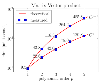
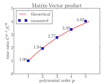
Fig. 3: Matrix-Vector product

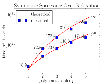
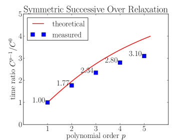
Fig. 4: Symmetric Successive Over Relaxation

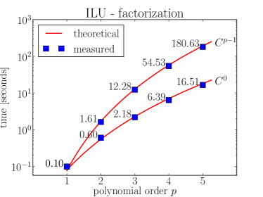
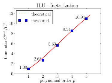
(a) factorization

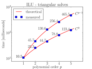
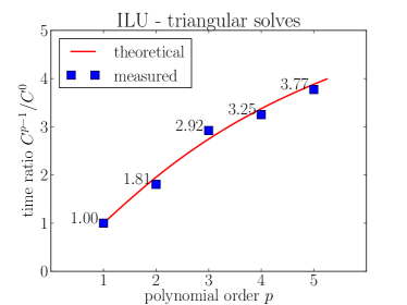
(b) triangular solves

Fig. 5: Incomplete LU

Overall, the measurements match closely the theoretical estimates except for SSOR sweeps. In the case of SSOR, forward and backward sweeps operate on the lower and upper triangular parts of the sparse matrix. Furthermore, the backward sweep is performed in reversed row ordering. The data access pattern is much more irregular than the one in matrix-vector product and causes greater miss rates in the processor cache. This situation leads to lower FLOP rates, hindering performance. Textbook implementations of ILU factorization and forward/backward triangular solves also suffer from this issue. However, PETSc employs a different data layout to store the LU factors and is able to achieve a FLOP rate comparable to the one for matrix-vector products. See [24] for a thorough analysis and discussion about the importance of data layout in triangular solves.

4.2 Iteration Counts

The purpose of a preconditioner is to improve the spectrum of the eigenvalues of the original operator. The number of iterations required for convergence is tightly related to this spectrum [18]. While the setup and application cost of the preconditioner is an important factor, a measure of how well preconditioners work in terms of number of iterations is also critical. In tables 6 and 7, we present numerical results which test how well each preconditioner works in terms of number of iterations.

We study the iteration counts as the function spaces vary in $h$ and $p$. In this study we interpret $h$ as half of the basis support size as opposed to the traditional interpretation of the element size, denoted as $h_{e}$. This means that $h$ retains its original meaning in the case of $C^{0}$ spaces, that is $h=h_{e}$. However, for $C^{p-1}$ spaces, $h=\left.h_{e}(p+1)\middle/2\right.$. We argue this based on the observation that under this definition, the condition number scales as standard theory suggests ($h^{-2}$, [3]) for the Laplace problem. If one considers scaling of the condition number based on $h_{e}$, the integration support, then the scaling artificially appears to be better.

Table 6: Number of iterations required for convergence of CG using different preconditioners and $C^{0}$ B-spline spaces

		Basis support size, $h$
$p$	type	$\left.1\middle/2\right.$	$\left.1\middle/4\right.$	$\left.1\middle/8\right.$	$\left.1\middle/16\right.$
1	Jacobi	5	11	23	45
2	Jacobi	19	31	42	61
3	Jacobi	68	91	97	107
4	Jacobi	216	355	406	424
1	SSOR	5	7	14	24
2	SSOR	11	14	17	27
3	SSOR	27	30	31	37
4	SSOR	65	75	77	80
1	ILU	1	7	12	22
2	ILU	7	9	15	26
3	ILU	8	11	19	34
4	ILU	10	14	24	42
1	EBE	6	21	30	45
2	EBE	17	34	45	65
3	EBE	23	38	50	86
4	EBE	27	47	63	111

Table 7: Number of iterations required for convergence of CG using different preconditioners and $C^{p-1}$ B-spline spac es. The BBB preconditioner is shown for $r=\left.p\middle/2\right.$.

		Basis support size, $h$
$p$	type	$\left.1\middle/2\right.$	$\left.1\middle/4\right.$	$\left.1\middle/8\right.$	$\left.1\middle/16\right.$
1	Jacobi	5	11	23	45
2	Jacobi	22	30	39	65
3	Jacobi	70	99	100	105
4	Jacobi	165	139	149	152
1	SSOR	5	7	14	24
2	SSOR	13	15	19	29
3	SSOR	33	34	34	41
4	SSOR	82	68	65	66
1	ILU	1	7	12	22
2	ILU	5	7	12	22
3	ILU	6	7	12	20
4	ILU	6	8	12	20
1	EBE	6	21	30	45
2	EBE	26	45	51	60
3	EBE	50	74	81	89
4	EBE	77	109	116	123
1	BBB	5	11	23	45
2	BBB	18	22	26	42
3	BBB	30	35	38	54
4	BBB	29	32	36	51

In both spaces, the remarkable result is that the ILU preconditioner outperforms other options in terms of number of iterations as well as the $p$ scaling. Of greater interest is that in the case of $C^{p-1}$ spaces, its $p$ scalability is perfect. While no theory currently exists to prove that the ILU preconditioner will lead to a converged result, it is among the most economical preconditioners to setup and apply to linear systems in the range of problems solved.

Our interest in studying the cost of solving medium-size problems using standard techniques is at the core of more complex preconditioning approaches such as domain-decomposition and multigrid. For example, despite the fact that ILU does not scale as well in $h$, we can use it in a multigrid approach to remove $h$ dependence. For example, in table 8 we show iteration counts for a two grid solver we constructed. On the fine grid, we use CG with ILU and a direct solver on the coarse level. The coarse level is a factor of $2^{3}$ unrefined in $h$ from the fine level. We see that as in standard $C^{0}$ spaces, a multigrid approach is able to remove $h$ dependence from linear systems discretized using $C^{p-1}$ spaces.

Table 8: Number of iterations required for convergence with a two grid solver

		Basis support size, $h$
$p$	space	$\left.1\middle/2\right.$	$\left.1\middle/4\right.$	$\left.1\middle/8\right.$	$\left.1\middle/16\right.$
1	$C^{0}$	4	16	19	19
2	$C^{0}$	15	18	20	21
3	$C^{0}$	18	20	21	22
4	$C^{0}$	20	24	25	26
1	$C^{0}$	4	16	19	19
2	$C^{1}$	14	15	17	19
3	$C^{2}$	14	15	18	19
4	$C^{3}$	14	15	18	19

The iteration counts for the BBB preconditioner shown in table 7 are for an overlap parameter $r=\left.p\middle/2\right.$. We have selected this size in an attempt to balance the cost of applying the preconditioner and its convergence. In table 9, we show convergence results for more choices of the overlap parameter $r$. Note that when $r=0$ the preconditioner is diagonal Jacobi. As the overlap increases, we see an improvement in the number of iterations. However, when the overlap is at its maximum, $r=p$, the setup and application of the preconditioner is prohibitively expensive. We suggest that the choice $r=\left.p\middle/2\right.$ leads to a good compromise between fast convergence and moderate application cost.

Table 9: Convergence results for the BBB preconditioner where the basis support size a constant $h=0.25$ and the overlap $r$ varies. Underlined entries represent a preconditioner with approximately the same number of nonzero entries as the original system matrix.

	Basis overlap, $r$
$p$	0	1	2	3	4
1	11	16
2	30	22	21
3	99	35	25	24
4	139	56	32	28	27
5	345	76	48	35	30
6	353	112	68	48	35
7	610	167	104	64	43
8	737	201	130	92	65

4.3 Timing Results

While the number of iterations required for convergence is a useful measure to study, it is not sufficient to understand which preconditioning options are better from a practical point of view. Frequently, a practitioner must experiment with different options on a meaningful range of problem sizes. For a preconditioner to be effective, the cost of setting up and applying must be weighted against its capability to improve the spectrum of eigenvalues, effectively reducing the total number of iterations.

We first present some timing results for linear systems consisting of $10^{5}$ degrees of freedom. In figure 6 we display bar graphs representing the total solution time required for convergence for different preconditioning options and varying polynomial order $p$. In each plot we display $C^{0}$ spaces on the left and $C^{p-1}$ on the right. Furthermore, each bar is divided into two parts. The bottom part represents the setup time required for each preconditioner and the top the remaining solve time. We also include the number of iterations required for convergence on the top of each bar.

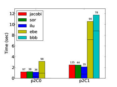
(a) $p=2$

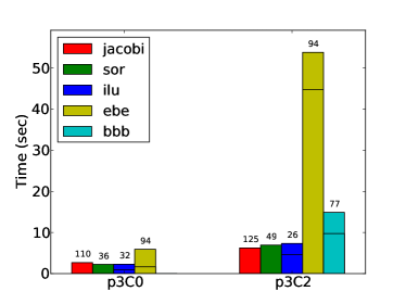
(b) $p=3$

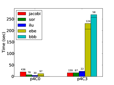
(c) $p=4$

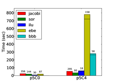
(d) $p=5$

Fig. 6: Solution times of various preconditioning options for $C^{0}$ and $C^{p-1}$ spaces consisting of $N=10^{5}$ degrees of freedom.

Most striking is the time required by the EBE and BBB preconditioners for $C^{p-1}$ spaces. As predicted in the theoretical estimates for setup cost, these preconditioners are considerably more expensive to setup, and additionally they are not able to significantly reduce the total number of iterations. This is an effect that continues to grow as we increase $N$, the size of the problem.

We would like to make an additional comment on the ILU preconditioner. From the analysis of setup costs, it is clear that EBE and BBB preconditioners are $p^{3}$ times more expensive to setup than ILU. However, the EBE, BBB, and ILU preconditioners are all based on the Gaussian elimination process. The EBE and BBB preconditioners are built by taking into account the interaction between a compact neighborhood of DOF (defined by elements in the case of EBE and by the overlap $r$ in the case of BBB). Due to its algorithmic structure, we intuitively argue that ILU is able to capture the interactions between different DOF in a more global manner, and therefore has a better effect on the convergence of the problem.

In figure 7 we remove the EBE and BBB preconditioning to better highlight the differences between the remaining choices. Also, we have increased the number of DOF to $10^{6}$. We see that in this case, the remaining preconditioners (Jacobi, SSOR, and ILU) all perform similarly in terms of time. We also see that SSOR and ILU require a similar number of iterations. We also note that the $C^{p-1}$ spaces are two times as expensive than the $C^{0}$ spaces for $p=2$ and three times as expensive for $p=3$, as predicted by our theoretical estimates.

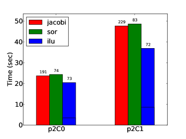
(a) $p=2$

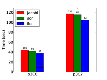
(b) $p=3$

Fig. 7: Solution times of various preconditioning options for $C^{0}$ and $C^{p-1}$ spaces consisting of $N=10^{6}$ degrees of freedom.

We extend the study to include a range of degrees of freedom in figure 8a, however we only consider the ILU preconditioner. We show the ratio of solve times for $C^{p-1}$ to $C^{0}$ for a range of problem sizes $N$ and polynomial orders $p$. We highlight that for this example, the cost of the use of the higher continuous basis is anywhere from $p$ to $2p$ times more expensive. However, in the theory section, we showed that the solve cost can be greatly reduced when using static condensation and solving the skeleton problem. In figure 8b we have repeated the numerical experiment, this time using static condensation on the $C^{0}$ spaces. Note that the additional assembly time incurred due to static condensation operations have been included into the solve cost. In this case, the $C^{p-1}$ spaces are $\mathcal{O}(p^{2})$ times more expensive to solve, as predicted by the theoretical cost of the matrix-vector multiplication estimates.

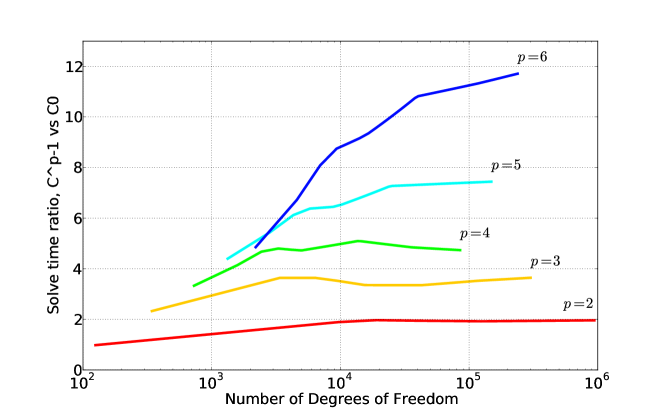
(a) $C^{p-1}$ versus $C^{0}$

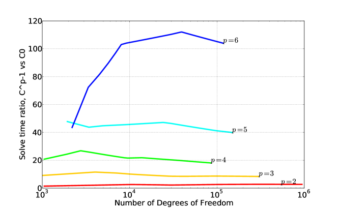
(b) $C^{p-1}$ versus $C^{0}$ with static condensation

Fig. 8: Solve time ratios for $C^{p-1}$ and $C^{0}$ spaces using CG preconditioned with ILU. Solve time is inclusive of the setup of the preconditioner but excludes assembly time. In the case of static condensation, the solve time includes extra assembly time required to compute the Schur complements.

5 Conclusions

We have presented a study on the additional cost incurred in the iterative solver due to the use of a more continuous basis in a Galerkin weak form. We have presented theoretical estimates for computational costs of matrix-vector multiplication as well as preconditioner setup and application for a variety of preconditioning techniques. We present numerical results for the Laplace problem to establish a baseline understanding of how continuity affects the solver.

We conclude that the matrix-vector product is at most eight times more expensive for the $C^{p-1}$ spaces. However, when using high $p$ with static condensation, this factor increases to $\left.8p^{2}\middle/33\right.$. We expect that the improved approximability per DOF of the $C^{p-1}$ spaces may be better realized when using the iterative solver, particularly for low $p$. This is, however, strongly tied to the performance of the selected preconditioner applied to the equation of interest.

We observe that for moderate $N$ and the Laplace problem, that the EBE and BBB preconditioners are prohibitively expensive options for $C^{p-1}$ spaces. This is because there is an element per basis function which results in far greater setup costs than in $C^{0}$ spaces. For these options to be effective for a particular problem, they should lead to a considerably large decrease in iterations compared to other options. This is not the case for the simple Laplace problem and, intuitively, we do not expect this to be the case for more complex applications.

The ILU preconditioner, while lacking a theoretical ground for convergence, performs quite well in terms of iterations and computational time. Remarkably, for $C^{p-1}$ spaces we observe perfect almost $p$-scaling of the preconditioned operator condition number up to $10^{6}$ degrees of freedom.

References

- [1] Mark Ainsworth, A hierarchical domain decomposition preconditioner for - finite element approximation on locally refined meshes, SIAM Journal on Scientific Computing, 17 (1996), pp. 1395–1413.
- [2] Douglas N. Arnold, Richard S. Falk, and Ragnar Winther, Multigrid in h (div) and h (curl), Numerische Mathematik, 85 (2000), pp. 197–217. 10.1007/PL00005386.
- [3] Owe Axelsson, Iteration number for the conjugate gradient method, Math. Comput. Simul., 61 (2003), pp. 421–435.
- [4] Satish Balay, Kris Buschelman, Victor Eijkhout, William D. Gropp, Dinesh Kaushik, Matthew G. Knepley, Lois Curfman McInnes, Barry F. Smith, and Hong Zhang, PETSc users manual, Tech. Report ANL-95/11 - Revision 3.0.0, Argonne National Laboratory, 2008.
- [5] Satish Balay, Kris Buschelman, William D. Gropp, Dinesh Kaushik, Matthew G. Knepley, Lois Curfman McInnes, Barry F. Smith, and Hong Zhang, PETSc Web page, 2010. http://www.mcs.anl.gov/petsc.
- [6] Nathan Collier, David Pardo, Lisandro Dalcin, Maciej Paszynski, and V.M. Calo, The cost of continuity: A study of the performance of isogeometric finite elements using direct solvers, Computer Methods in Applied Mechanics and Engineering, 213–216 (2012), pp. 353 Р361.
- [7] J. Austin Cottrell, T. J. R. Hughes, and Yuri Bazilevs, Isogeometric Analysis: Toward Unification of CAD and FEA, John Wiley and Sons, 2009.
- [8] L. Beirao da Veiga, D. Cho, L. Pavarino, and S. Scacchi, Overlapping schwarz methods for isogeometric analysis, tech. report, Istituto di Matematica Applicata e Tecnologie Informatiche, 2011.
- [9] Lisandro D. Dalcin, Rodrigo R. Paz, Pablo A. Kler, and Alejandro Cosimo, Parallel distributed computing using python, Advances in Water Resources, 34 (2011), pp. 1124 – 1139.
- [10] Luca Dedè, T. J. R. Hughes, Scott Lipton, and V. M. Calo, Structural topology optimization with isogeometric analysis in a phase field approach, in USNCTAM2010, 16th US National Congree of Theoretical and Applied Mechanics, 2010.
- [11] I. S. Duff and J. K. Reid, The multifrontal solution of indefinite sparse symmetric linear, ACM Trans. Math. Softw., 9 (1983), pp. 302–325.
- [12] I. S. Duff and J. K. Reid, The multifrontal solution of unsymmetric sets of linear equations, SIAM Journal on Scientific and Statistical Computing, 5 (1984), pp. 633–641.
- [13] Hector Gomez, V. M. Calo, Yuri Bazilevs, and T. J. R. Hughes, Isogeometric analysis of the Cahn-Hilliard phase-field model, Computer Methods in Applied Mechanics and Engineering, 197 (2008), pp. 4333–4352.
- [14] H. Gomez, T. J. R. Hughes, X. Nogueira, and V. M. Calo, Isogeometric analysis of the isothermal Navier-Stokes-Korteweg equations, Computer Methods in Applied Mechanics and Engineering, 199 (2010), p. 1828.
- [15] T. J. R. Hughes, J.A. Cottrell, and Y. Bazilevs, Isogeometric analysis: CAD, finite elements, NURBS, exact geometry and mesh refinement, Computer Methods in Applied Mechanics and Engineering, 194 (2005), pp. 4135–4195.
- [16] John D. Hunter, Matplotlib: A 2D graphics environment, Computing In Science & Engineering, 9 (2007), pp. 90–95.
- [17] J. D. McCalpin, STREAM: Sustainable memory bandwidth in high performance computers, tech. report, University of Virginia, 2011. http://www.cs.virginia.edu/stream.
- [18] Noel Nachtigal, Satish C. Redyy, and Lloyd N. Trefethen, How fast are nonsymmetric matrix iterations?, SIAM Journal of Matrix Analysis and Applications, 13 (1992), pp. 778–795.
- [19] Travis E. Oliphant, Guide to NumPy, Trelgol Publishing, 2006.
- [20] David Pardo, Integration of -adaptivity with a two grid solver: application to electromagnetics, PhD thesis, University of Texas at Austin, 2004.
- [21] Yousef Saad, Iterative methods for sparse linear systems, Society for Industrial and Applied Mathematics, 2nd ed., 2003.
- [22] Jonathan Richard Shewchuk, An introduction to the conjugate gradient method without the agonizing pain. online, Aug 1994. http://www.cs.cmu.edu/ quake-papers/painless-conjugate-gradient.pdf.
- [23] Barry Smith, Petter Bjorstad, and William Gropp, Domain decomposition: parallel methods for elliptic partial differential equations, Cambridge University Press, 1996.
- [24] B. Smith and H. Zhang, Sparse triangular solves for ILU revisited: Data layout crucial to better performance, International Journal of High Performance Computing Applications, 25 (2010), pp. 386–391.
- [25] SymPy Development Team, SymPy: Python library for symbolic mathematics, 2012.
- [26] Edward L. Wilson, The static condensation algorithm, International Journal for Numerical Methods in Engineering, 8 (1974), pp. 198–203.