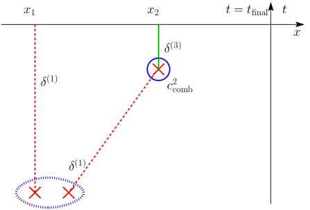
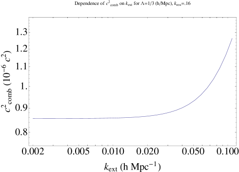
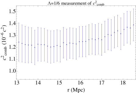
SU-ITP-12/17

The Effective Field Theory
of Cosmological Large Scale Structures

John Joseph M. Carrasco1, Mark P. Hertzberg1,2, Leonardo Senatore1,2

1 Stanford Institute for Theoretical Physics and Department of Physics,
Stanford University, Stanford, CA 94306

2 Kavli Institute for Particle Astrophysics and Cosmology,
Stanford University and SLAC, Menlo Park, CA 94025

  Abstract
Large scale structure surveys will likely become the next leading cosmological probe. In our universe, matter perturbations are large on short distances and small at long scales, i.e. strongly coupled in the UV and weakly coupled in the IR. To make precise analytical predictions on large scales, we develop an effective field theory formulated in terms of an IR effective fluid characterized by several parameters, such as speed of sound and viscosity. These parameters, determined by the UV physics described by the Boltzmann equation, are measured from N𝑁N-body simulations. We find that the speed of sound of the effective fluid is cs2106c2superscriptsubscript𝑐𝑠2superscript106superscript𝑐2c_{s}^{2}\approx 10^{-6}c^{2} and that the viscosity contributions are of the same order. The fluid describes all the relevant physics at long scales k𝑘k and permits a manifestly convergent perturbative expansion in the size of the matter perturbations δ(k)𝛿𝑘\delta(k) for all the observables. As an example, we calculate the correction to the power spectrum at order δ(k)4𝛿superscript𝑘4\delta(k)^{4}. The predictions of the effective field theory are found to be in much better agreement with observation than standard cosmological perturbation theory, already reaching percent precision at this order up to a relatively short scale k0.24hsimilar-to-or-equals𝑘0.24k\simeq 0.24h Mpc-1.
 

1 Introduction

Large Scale Structure Surveys have the potential of becoming the leading cosmological observable in the next decade. They contain a tremendous amount of cosmological information. If we were able to extract information from all the modes that go from the horizon scale 104similar-toabsentsuperscript104\sim 10^{4} Mpc to the non-linear scale 10similar-toabsent10\sim 10 Mpc, we would obtain about

(10410)3109similar-tosuperscriptsuperscript104103superscript109\left(\frac{10^{4}}{10}\right)^{3}\sim 10^{9} (1)

independent modes. The Planck satellite in comparison has about (2×10³)2106similar-tosuperscript2superscript1032superscript106(2\times 10^{3})^{2}\sim 10^{6} modes. Of course, accessing all this information is much harder than for the CMB, due to the short scale non-linearities. There are several aspects to this problem. The first problem is related to our currently limited understanding of the evolution of dark matter on large scales. Non-linear corrections are very important even on scales larger than 101010 Mpc, because modes of different wavelengths couple to each other. Understanding these corrections is a problem that affects all large scale structure observables. There are then two additional issues that affect most, but at least not all, observables. One is the fact that most dark matter is clumped in very non-linear structures (dark matter halos); and the other is the fact that what we often observe are galaxies, and not just dark matter halos, and not even dark matter long wavelength perturbations. The solution to these two last problems requires the correct understanding of the so-called halo- and galaxy- biases. These two problems, while important and deeply interesting in their own right, are very astrophysical in nature, and we do not address them here.

Instead here we try to address in a rigorous way the first problem, that is the prediction of the dark matter distribution on scales larger than the non-linear scale. The fact that the universe is characterized by two well separated scales, the Hubble scale, over which perturbations are linear, and the non-linear scale, which indeed characterizes the scale over which gravitational collapse overtakes the expansion of the universe, makes the problem amenable to an Effective Field Theory (EFT) treatment. An effective theory is a description of a system that captures all the relevant degrees of freedom and describes all the relevant physics at a macroscopic scale of interest. The short distance (so called ultraviolet or ‘UV’) physics is integrated out and affects the effective field theory only through various couplings in a perturbative expansion in the ratio of microphysical UV scale/s to the macroscopic scale being probed. This technique has been systematically used in particle physics and condensed matter physics for many years, but has not been fully used in astrophysics and cosmology. An important early (and recent) application of these techniques in cosmology is the so-called Effective Field Theory of Inflation [1]. In a similar vein, understanding the large scale properties of the universe is very important, and is ready for a careful analysis.

Indeed the situation in the universe is very similar to what happens in the chiral Lagrangian that describes pion interactions in Particle Physics. At very low energies, pions are weakly interacting. These interactions and the size of the fluctuations grow with energy until we hit the Quantum ChromoDynamics (QCD) scale, 4πFπsimilar-toabsent4𝜋subscript𝐹𝜋\sim 4\pi F_{\pi}, at which the pions become strongly coupled. The Chiral Lagrangian [2] offers the correct effective theory allowing arbitrarily precise predictions, up to non-perturbative effects, at energies E4πFπmuch-less-than𝐸4𝜋subscript𝐹𝜋E\ll 4\pi F_{\pi}. In our universe, matter fluctuations are small at large distances and becomes larger and larger as we move up to the non-linear scale. Since the size of the non-linear terms, which are nothing but interactions, grows with the size of the fluctuations, we see that at long distances the universe should be described by some weakly coupled degree of freedom, that becomes more and more interacting as we move closer to the non-linear scale, at which point the fluctuations become strongly coupled. The coupling constant should indeed be represented by the ratio of the considered wavenumber k𝑘k over the wavenumber at the non-linear scale kNLsubscript𝑘𝑁𝐿k_{NL}: k/kNL𝑘subscript𝑘𝑁𝐿k/k_{NL}. Notice that indeed the size of the density perturbations δρ/ρ𝛿𝜌𝜌\delta\rho/\rho on a scale k𝑘k scales as (k/kNL)2superscript𝑘subscript𝑘𝑁𝐿2(k/k_{NL})^{2}. This scaling suggests the existence of an effective field theory that should allow us to describe with arbitrary precision the universe on scales kkNLmuch-less-than𝑘subscript𝑘𝑁𝐿k\ll k_{NL}, very much as the Chiral Lagrangian represents the right effective field theory to describe pion dynamics to arbitrary precision.

Such an effective theory would have particularly relevant observational implications. Already now, large scale structure surveys such as BOSS or DES are measuring the galaxy-galaxy correlation function, so called Baryon Acoustic Oscillations (BAO), at scales of order 100 Mpc. Next generation experiments such as LSST will measure this quantity at about percent precision. These observations contain huge amount of information on Dark Energy and on Inflation, through for example the non-Gaussianity of the primordial perturbations. The BAO scale is about one order of magnitude longer than the non-linear scale, where δρ/ρ102similar-to𝛿𝜌𝜌superscript102\delta\rho/\rho\sim 10^{-2}, and therefore physics at this scale must be describable by rigorous perturbative methods. The alternative is to rely on either time consuming numerical simulations, or on analytical approaches that however are limited by some irreducible mistake that is hard to quantify precisely. In an ideal situation, numerical N𝑁N-body simulations should be quickly done only at small scales, to describe phenomena affected by gravitational collapse, rather than running large simulations to describe weakly coupled physics. This has been indeed recently elucidated in the context of the bias, where it was shown that in order to derive the bias on large scales one needs to run very small simulations in a curved universe [3]. This line of reasoning is indeed very similar to what happens in QCD, where we perform lattice simulation to measure quantities relevant at energies above around one GeV, while we use the chiral Lagrangian for predictions at smaller energies.

The effective field theory (EFT) of the long distance universe was initially developed by some of us in [4]. It was noticed that by concentrating on length scales longer than the non-linear scale, the universe is described by a fluid with small perturbations. The equations of motion of this fluid are organized in a derivative expansion in the ratio of the considered wavenumber over the wavenumber associated to the non-linear scale kNL1/10similar-tosubscript𝑘𝑁𝐿110k_{NL}\sim 1/10 Mpc-1. At leading order in derivatives, the fluid has the stress tensor of an ordinary imperfect fluid, characterized by a speed of sound for the fluctuations, a bulk and a shear viscosity, plus a stochastic pressure component. This makes our approach different with respect to the ‘standard’ approaches both at a quantitative and a qualitative level.

The purpose of this paper is to further develop this effective theory and be able to make observational predictions. The parameters that characterize the fluid, the speed of sounds, bulk viscosity, etc., are determined by the microphysics at the non-linear scale, that we call UV, and cannot be derived from within the effective theory. They have to be either fit to observations, or measured in small N𝑁N-body simulations. At this point, the EFT becomes predictive. Again, this is very similar to what happens in QCD, where one can measure the pion coupling constant Fπsubscript𝐹𝜋F_{\pi} in lattice simulations, after which the Chiral Lagrangian becomes predictive.

Our basic method and key results are summarized as the following:

  • By smoothing the collisionless Boltzmann equation for non-relativistic matter in an expanding FRW background on a length scale Λ1superscriptΛ1\Lambda^{-1}, we establish the continuity and Euler equations for an effective fluid. The Euler equation includes an effective stress-tensor [τij]Λsubscriptdelimited-[]superscript𝜏𝑖𝑗Λ[\tau^{ij}]_{\Lambda} that is sourced by the short-modes δssubscript𝛿𝑠\delta_{s}.

  • By taking correlation functions of the stress tensor in the presence of long wavelength fluctuations, we define an effective stress-tensor that is only a function of the long wavelength fluctuations. It takes the form

    [τij]Λsubscriptdelimited-[]superscript𝜏𝑖𝑗Λ\displaystyle[\tau^{ij}]_{\Lambda} =\displaystyle\!\!= δijpb+ρb[cs2δijδlcbv2Haδijkvlk\displaystyle\!\!\delta^{ij}p_{b}+\rho_{b}\Bigg{[}c_{s}^{2}\,\delta^{ij}\delta_{l}-{c_{bv}^{2}\over Ha}\delta^{ij}\,\partial_{k}v_{l}^{k} (2)
    \displaystyle\!\!- 34csv2Ha(jvli+ivlj23δijkvlk)]+,\displaystyle\!\!{3\over 4}{c_{sv}^{2}\over Ha}\left(\partial^{j}v_{l}^{i}+\partial^{i}v_{l}^{j}-{2\over 3}\delta^{ij}\,\partial_{k}v_{l}^{k}\right)\Bigg{]}+\ldots\ ,

    where the various parameters cs2,cbv2superscriptsubscript𝑐𝑠2superscriptsubscript𝑐𝑏𝑣2c_{s}^{2},c_{bv}^{2} etc. are defined by proper correlation functions of short wavelength and long wavelength fluctuations.

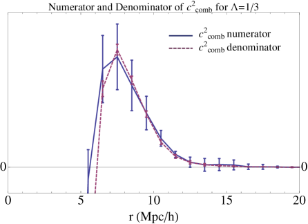
  • By directly evaluating the stress tensor from the microphysical theory, i.e., from N𝑁N-body simulations, and computing the appropriate correlation functions, we calculate the value of the fluid parameters. For a ΛΛ\LambdaCDM universe with standard cosmological parameters at redshift z=0𝑧0z=0 and smoothing scale Λ=1/3hΛ13\Lambda=1/3h Mpc-1, we find

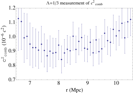
    ccomb2(Λ=1/3)superscriptsubscript𝑐comb2Λ13\displaystyle c_{\rm comb}^{2}{(\Lambda=1/3)} =0.96±0.1×10⁶(c2),absentplus-or-minus0.960.1superscript106superscript𝑐2\displaystyle=0.96\pm 0.1\times 10^{-6}\ (c^{2})\,, (3)

    where ccomb2subscriptsuperscript𝑐2combc^{2}_{\rm comb} is the combination of cs2,cbv2superscriptsubscript𝑐𝑠2superscriptsubscript𝑐𝑏𝑣2c_{s}^{2},c_{bv}^{2} and csv2superscriptsubscript𝑐𝑠𝑣2c_{sv}^{2} that is relevant for the leading non-linear correction to the power spectrum (one-loop in perturbation theory), and c𝑐c is the speed of light.

  • Alternatively, by directly matching the couplings of the effective fluid to the measured power spectrum, we obtain ccomb2(Λ=1/3)0.9×106c2similar-to-or-equalssuperscriptsubscript𝑐comb2Λ130.9superscript106superscript𝑐2c_{\rm comb}^{2}{(\Lambda=1/3)}\simeq 0.9\times 10^{-6}c^{2} in remarkable agreement with the direct measurement from N𝑁N-body simulations.

  • The fluid parameters carry ΛΛ\Lambda dependence (as does any ‘bare’ parameter in an interacting field theory). This cutoff dependence is taken to cancel against the cutoff dependence of the loop integral. As usual in effective field theories, we ‘renormalize’ the theory by sending the cutoff ΛΛ\Lambda\to\infty and carefully changing the fluid parameters so that predictions at low wavenumbers are not changed in the process. The finite values of the fluid parameters such as ccomb2superscriptsubscript𝑐comb2c_{\rm comb}^{2} in the ΛΛ\Lambda\to\infty limit is a direct measure of the irreducible finite error made in standard approaches that approximate the dark matter on large scales as a pressureless ideal fluid. This is an irreducible error that is not recovered even by solving non-linearly the equations for a pressureless ideal fluid, as the various perturbative approaches attempt to do. This occurs simply because the equations they solve are not correct. Our approach, in contrast, should reach arbitrary precision, at least in principle, up to non-perturbative corrections.

  • The pressure and viscosity dampen the power spectrum by acting in opposition to gravity, which makes sense intuitively. This is able to help explain the observed shape of the baryon-acoustic-oscillations in the power spectrum relative to standard perturbation theory (SPT).

  • More precisely, at one-loop the density-density power spectrum receives a correction δP𝛿𝑃\delta P from the fluid parameters, which we find to be

    δP(k)ccomb2k2H2P11,l(k)similar-to𝛿𝑃𝑘superscriptsubscript𝑐comb2superscript𝑘2superscript𝐻2subscript𝑃11𝑙𝑘\delta P(k)\sim-c_{\rm comb}^{2}\frac{k^{2}}{H^{2}}P_{11,l}(k) (4)

    where P11,l(k)subscript𝑃11𝑙𝑘P_{11,l}(k) is the linear power spectrum. Since this is negative and grows as a function of k𝑘k, the power spectrum is reduced compared to SPT at high k𝑘k’s, improving the agreement with the full non-linear spectrum.

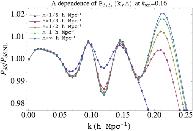
  • We will find that already at one-loop, the computed power spectrum agrees at percent level with the non-linear one up to k0.24hsimilar-to𝑘0.24k\sim 0.24h Mpc-1. This suggest that in large scale structure surveys we should be able to extract primordial information all the way to at least such an high wavenumber, improving greatly with respect to the CMB our knowledge of the origin of the universe.

During the years there has been a very large and relevant amount of work in understanding perturbatively the large scale clustering of dark matter. An incomplete sample of these works is given by [5, 6, 7, 8, 9, 10, 11, 12, 13, 14, 15, 16, 17, 18, 19, 20, 21, 22, 23, 24, 25].

2 From Dark Matter Particles to Cosmic Fluid

We take dark matter to be fundamentally described by a set of identical collisionless classical non-relativistic particles interacting only gravitationally. This is a very good approximation for all dark matter candidates apart from very light axions. Given that on large scales baryons follow dark matter, we can include them in the overall dark matter description. As we discuss later, we also neglect general relativistic effects and radiation effects. In this approximation, numerical N𝑁N-body simulations exactly solve our UV theory. The coefficients of our effective fluid can therefore be extracted directly from the N𝑁N-body simulations, following directly the procedure described in [4]. Here, the UV theory is described by a Boltzmann equation. Therefore, in order to be able to extract the fluid parameters from N𝑁N-body simulations, we need to derive the fluid equations from the Boltzmann equations and subsequently express the parameters of the effective fluid directly in terms of quantities measurable in an N𝑁N-body simulation. This is the task of this section.

2.1 Boltzmann Equation

Let us start from a one-particle phase space density fn(x,p)subscript𝑓𝑛𝑥𝑝f_{n}(\vec{x},\vec{p}) such that fn(x,p)d3xd3psubscript𝑓𝑛𝑥𝑝superscript𝑑3𝑥superscript𝑑3𝑝f_{n}(\vec{x},\vec{p})d^{3}xd^{3}p represents the probability for the particle n𝑛n to occupy the infinitesimal phase space volume d3xd3psuperscript𝑑3𝑥superscript𝑑3𝑝d^{3}xd^{3}p. For a point particle, we have

fn(x,p)=δ(3)(xxn)δ(3)(pmavn).subscript𝑓𝑛𝑥𝑝superscript𝛿3𝑥subscript𝑥𝑛superscript𝛿3𝑝𝑚𝑎subscript𝑣𝑛f_{n}(\vec{x},\vec{p})=\delta^{(3)}(\vec{x}-\vec{x}_{n})\delta^{(3)}(\vec{p}-m\,a\,\vec{v}_{n})\ . (5)

The total phase space density f𝑓f is defined such that f(x,p)d3xd3p𝑓𝑥𝑝superscript𝑑3𝑥superscript𝑑3𝑝f(\vec{x},\vec{p})d^{3}xd^{3}p is the probability that there is a particle in the infinitesimal phase space volume d3xd3psuperscript𝑑3𝑥superscript𝑑3𝑝d^{3}xd^{3}p:

f(x,p)=nδ(3)(xxn)δ(3)(pmavn).𝑓𝑥𝑝subscript𝑛superscript𝛿3𝑥subscript𝑥𝑛superscript𝛿3𝑝𝑚𝑎subscript𝑣𝑛f(\vec{x},\vec{p})=\sum_{n}\delta^{(3)}(\vec{x}-\vec{x}_{n})\delta^{(3)}(\vec{p}-m\,a\,\vec{v}_{n})\ . (6)

We define the mass density ρ𝜌\rho, the momentum density πisuperscript𝜋𝑖\pi^{i} and the kinetic tensor σijsuperscript𝜎𝑖𝑗\sigma^{ij} as

ρ(x,t)=ma3d3pf(x,p)=ma3nδ(3)(xxn),𝜌𝑥𝑡𝑚superscript𝑎3superscript𝑑3𝑝𝑓𝑥𝑝𝑚superscript𝑎3subscript𝑛superscript𝛿3𝑥subscript𝑥𝑛\displaystyle\rho(\vec{x},t)=\frac{m}{a^{3}}\int d^{3}p\;f(\vec{x},\vec{p})=\frac{m}{a^{3}}\sum_{n}\delta^{(3)}(\vec{x}-\vec{x}_{n})\ , (7)
πi(x,t)=1a4d3ppif(x,p)=ma3nvniδ(3)(xxn),superscript𝜋𝑖𝑥𝑡1superscript𝑎4superscript𝑑3𝑝superscript𝑝𝑖𝑓𝑥𝑝𝑚superscript𝑎3subscript𝑛superscriptsubscript𝑣𝑛𝑖superscript𝛿3𝑥subscript𝑥𝑛\displaystyle\pi^{i}(\vec{x},t)=\frac{1}{a^{4}}\int d^{3}p\;p^{i}f(\vec{x},\vec{p})=\frac{m}{a^{3}}\sum_{n}v_{n}^{i}\delta^{(3)}(\vec{x}-\vec{x}_{n})\ , (8)
σij(x,t)=1ma5d3ppipjf(x,p)=nma3vnivnjδ(3)(xxn).superscript𝜎𝑖𝑗𝑥𝑡1𝑚superscript𝑎5superscript𝑑3𝑝superscript𝑝𝑖superscript𝑝𝑗𝑓𝑥𝑝subscript𝑛𝑚superscript𝑎3subscriptsuperscript𝑣𝑖𝑛subscriptsuperscript𝑣𝑗𝑛superscript𝛿3𝑥subscript𝑥𝑛\displaystyle\sigma^{ij}(\vec{x},t)=\frac{1}{ma^{5}}\int d^{3}p\;p^{i}p^{j}f(\vec{x},\vec{p})=\sum_{n}\frac{m}{a^{3}}v^{i}_{n}v^{j}_{n}\delta^{(3)}(\vec{x}-\vec{x}_{n})\ .

The particle distribution fnsubscript𝑓𝑛f_{n} evolves accordingly to the Boltzmann equation

DfnDt=fnt+pma2fnxmn¯nϕn¯xfnp=0,𝐷subscript𝑓𝑛𝐷𝑡subscript𝑓𝑛𝑡𝑝𝑚superscript𝑎2subscript𝑓𝑛𝑥𝑚subscript¯𝑛𝑛subscriptitalic-ϕ¯𝑛𝑥subscript𝑓𝑛𝑝0\frac{Df_{n}}{Dt}=\frac{{\partial}f_{n}}{{\partial}t}+\frac{\vec{p}}{ma^{2}}\cdot\frac{{\partial}f_{n}}{{\partial}\vec{x}}-m\sum_{\bar{n}\neq n}\frac{{\partial}\phi_{\bar{n}}}{{\partial}\vec{x}}\cdot\frac{{\partial}f_{n}}{{\partial}\vec{p}}=0\ , (9)

where ϕnsubscriptitalic-ϕ𝑛\phi_{n} is the single-particle Newtonian potential. There are two important points to highlight about the former equation. First, we have taken the Newtonian limit of the full general relativistic Boltzmann equation. This is an approximation we make for simplicity. All our results can be trivially extended to include general relativistic effects. However, it is easy to realize that the Newtonian approximation is particularly well justified. Non-linear corrections to the evolution of the dark matter evolution are concentrated at short scales, with corrections that scale as k2/kNL2superscript𝑘2superscriptsubscript𝑘𝑁𝐿2k^{2}/k_{NL}^{2}. General relativistic corrections are expected to scale as k2/(aH)2superscript𝑘2superscript𝑎𝐻2k^{2}/(aH)^{2}. This means that we should be able to cover up to wavelength of order 300300300 Mpc before worrying about per mille General relativity corrections. Furthermore, one of the main goals of this paper is to recover the parameters of the effective fluid of the universe from very short scale simulations valid on distances of order of the non-linear scale. The parameters we will extract in the Newtonian approximation are automatically valid also for the description of an effective fluid coupled to gravity in the full general relativistic setting.

A second important point to highlight in the former Boltzmann equation is about the single-particle Newtonian potential ϕnsubscriptitalic-ϕ𝑛\phi_{n}. Following [4], the Newtonian potential ϕitalic-ϕ\phi is defined through the Poisson equation

2ϕ=4πGa2(ρρb),superscript2italic-ϕ4𝜋𝐺superscript𝑎2𝜌subscript𝜌𝑏{\partial}^{2}\phi=4\pi Ga^{2}\left(\rho-\rho_{b}\right)\ , (10)

with ρbsubscript𝜌𝑏\rho_{b} being the background density and 2=δijijsuperscript2superscript𝛿𝑖𝑗subscript𝑖subscript𝑗{\partial}^{2}=\delta^{ij}{\partial}_{i}{\partial}_{j}. We raise and lower spatial indexes with δijsubscript𝛿𝑖𝑗\delta_{ij}. The solution reads

ϕ=nϕn+4πGa2ρbμ2,italic-ϕsubscript𝑛subscriptitalic-ϕ𝑛4𝜋𝐺superscript𝑎2subscript𝜌𝑏superscript𝜇2\displaystyle\phi=\sum_{n}\phi_{n}+\frac{4\pi Ga^{2}\rho_{b}}{\mu^{2}}\ , (11)
ϕn(x)=Gm|xxn|eμ|xxn|.subscriptitalic-ϕ𝑛𝑥𝐺𝑚𝑥subscript𝑥𝑛superscript𝑒𝜇𝑥subscript𝑥𝑛\displaystyle\phi_{n}(\vec{x})=-\frac{G\,m}{|\vec{x}-\vec{x}_{n}|}e^{-\mu|\vec{x}-\vec{x}_{n}|}\ . (12)

Notice that the overall ϕ(x)italic-ϕ𝑥\phi(\vec{x}) is IR divergent in an infinite universe. This is due to a breaking of the Newtonian approximation. We have regulated it with an IR cutoff μ𝜇\mu that we will take to zero at the end of the calculation. Our results do not depend on μ𝜇\mu, as indeed we are interested in very short distance physics.

By summing over n𝑛n, we obtain the Boltzmann equation for f𝑓f

DfDt=ft+pma2fxmn,n¯;n¯nϕn¯xfnp=0.𝐷𝑓𝐷𝑡𝑓𝑡𝑝𝑚superscript𝑎2𝑓𝑥𝑚subscript𝑛¯𝑛¯𝑛𝑛subscriptitalic-ϕ¯𝑛𝑥subscript𝑓𝑛𝑝0\frac{Df}{Dt}=\frac{{\partial}f}{{\partial}t}+\frac{\vec{p}}{ma^{2}}\cdot\frac{{\partial}f}{{\partial}\vec{x}}-m\sum_{n,\bar{n};\bar{n}\neq n}\frac{{\partial}\phi_{\bar{n}}}{{\partial}\vec{x}}\cdot\frac{{\partial}f_{n}}{{\partial}\vec{p}}=0\ . (13)

2.2 Smoothing

Following [4], we construct the equations of motion for the effective fluid by smoothing the Boltzmann equations and by taking moments of the resulting long-distance Boltzmann equation. The smoothing guarantees that the Boltzmann hierarchy can be truncated, leaving us with an effective fluid. indeed, notice that it is not trivial at all that we should end up with an effective fluid. Fluid equations are usually valid over distances longer than the mean free path of the particles. But here for dark matter particles the mean free path is virtually infinite. What saves us is that the dark matter particles have had a finite amount of proper time, of order H1superscript𝐻1H^{-1}, to travel since reheating, and they traveled at a very non-relativistic speed. This defines a length scale vH11/kNLsimilar-to𝑣superscript𝐻11subscript𝑘𝑁𝐿vH^{-1}\sim 1/k_{NL} which is indeed of order of the non-linear scale. This length scale plays the role of a mean free path, as verified in [4]. The truncation of the Boltzmann hierarchy is regulated by powers k/kNL1much-less-than𝑘subscript𝑘𝑁𝐿1k/k_{NL}\ll 1.

We define the Gaussian smoothing

WΛ(x)=(Λ2π)3e12Λ2x2,WΛ(k)=e12k2Λ2,formulae-sequencesubscript𝑊Λ𝑥superscriptΛ2𝜋3superscript𝑒12superscriptΛ2superscript𝑥2subscript𝑊Λ𝑘superscript𝑒12superscript𝑘2superscriptΛ2W_{\Lambda}(\vec{x})=\left(\frac{\Lambda}{\sqrt{2\pi}}\right)^{3}e^{-\frac{1}{2}\Lambda^{2}x^{2}}\ ,\qquad W_{\Lambda}(k)=e^{-\frac{1}{2}\frac{k^{2}}{\Lambda^{2}}}\ , (14)

with Λ2superscriptΛ2\Lambda^{2} representing a k𝑘k-space, comoving cutoff scale. This will smooth out quantities with wavenumber kΛgreater-than-or-equivalent-to𝑘Λk\gtrsim\Lambda, or equivalently with waveleghts smaller than λ1/Λless-than-or-similar-to𝜆1Λ\lambda\lesssim 1/\Lambda. We regularize our observable quantities 𝒪(x,t)𝒪𝑥𝑡{\cal O}(\vec{x},t), ρ,π,ϕ,𝜌𝜋italic-ϕ\rho,\pi,\phi,\ldots , by taking convolutions in real space with the filter, defining long-wavelength quantities as

𝒪l(x,t)=[𝒪]Λ(x,t)=d3xWΛ(xx)𝒪(x).subscript𝒪𝑙𝑥𝑡subscriptdelimited-[]𝒪Λ𝑥𝑡superscript𝑑3superscript𝑥subscript𝑊Λ𝑥superscript𝑥𝒪superscript𝑥{\cal O}_{l}(\vec{x},t)=\left[{\cal O}\right]_{\Lambda}(\vec{x},t)=\int d^{3}x^{\prime}\,W_{\Lambda}(\vec{x}-\vec{x}^{\prime}){\cal O}(\vec{x}^{\prime})\ . (15)

Notice that in Fourier space W(k)1𝑊𝑘1W(k)\rightarrow 1 as k0𝑘0k\rightarrow 0: our fields are asymptotically untouched at long distances.

The smoothed Boltzmann equation becomes

[DfDt]Λ=flt+pma2flxmn,n¯,nn¯d3xWΛ(xx)ϕnx(x)fn¯p.subscriptdelimited-[]𝐷𝑓𝐷𝑡Λsubscript𝑓𝑙𝑡𝑝𝑚superscript𝑎2subscript𝑓𝑙𝑥𝑚subscript𝑛¯𝑛𝑛¯𝑛superscript𝑑3superscript𝑥subscript𝑊Λ𝑥superscript𝑥subscriptitalic-ϕ𝑛superscript𝑥superscript𝑥subscript𝑓¯𝑛𝑝\left[\frac{Df}{Dt}\right]_{\Lambda}=\frac{{\partial}f_{l}}{{\partial}t}+\frac{\vec{p}}{ma^{2}}\cdot\frac{{\partial}f_{l}}{{\partial}\vec{x}}-m\sum_{n,\bar{n},n\neq\bar{n}}\int d^{3}x^{\prime}W_{\Lambda}(\vec{x}-\vec{x}^{\prime})\frac{{\partial}\phi_{n}}{{\partial}\vec{x}^{\prime}}(\vec{x}^{\prime})\cdot\frac{{\partial}f_{\bar{n}}}{{\partial}\vec{p}}\ . (16)

Fluid equations are obtained by taking successive moments

d3ppi1pin[DfDt]Λ(x,p)=0,superscript𝑑3𝑝superscript𝑝subscript𝑖1superscript𝑝subscript𝑖𝑛subscriptdelimited-[]𝐷𝑓𝐷𝑡Λ𝑥𝑝0\int d^{3}p\;p^{i_{1}}\ldots p^{i_{n}}\left[\frac{Df}{Dt}\right]_{\Lambda}(\vec{x},\vec{p})=0\ , (17)

creating in this way a set of coupled differential equations known as Boltzmann hierarchy. As we will explain in more detail later, it will be sufficient for the purposes this paper to stop at the first two moments (one-loop approximation). The first two moments will give the continuity and momentum equations in the approximation in which the fluid is described by the Navier-Stokes approximation, with the addition of a stochastic term. We obtain

ρ˙l+3Hρl+1ai(ρlvli)=0,subscript˙𝜌𝑙3𝐻subscript𝜌𝑙1𝑎subscript𝑖subscript𝜌𝑙superscriptsubscript𝑣𝑙𝑖0\displaystyle\dot{\rho}_{l}+3H\rho_{l}+\frac{1}{a}{\partial}_{i}(\rho_{l}v_{l}^{i})=0\ , (18)
v˙li+Hvli+1avljjvli+1aiϕl=1aρlj[τij]Λ.superscriptsubscript˙𝑣𝑙𝑖𝐻superscriptsubscript𝑣𝑙𝑖1𝑎superscriptsubscript𝑣𝑙𝑗subscript𝑗superscriptsubscript𝑣𝑙𝑖1𝑎subscript𝑖subscriptitalic-ϕ𝑙1𝑎subscript𝜌𝑙subscript𝑗subscriptdelimited-[]superscript𝜏𝑖𝑗Λ\displaystyle\dot{v}_{l}^{i}+Hv_{l}^{i}+\frac{1}{a}v_{l}^{j}{\partial}_{j}v_{l}^{i}+\frac{1}{a}{\partial}_{i}\phi_{l}=-\frac{1}{a\rho_{l}}{\partial}_{j}\left[\tau^{ij}\right]_{\Lambda}\ . (19)

Let us define the various quantities that enter in these equations. We define the long wavelength velocity field as the ratio of the momentum and the density

vli=πliρl.superscriptsubscript𝑣𝑙𝑖superscriptsubscript𝜋𝑙𝑖subscript𝜌𝑙v_{l}^{i}=\frac{\pi_{l}^{i}}{\rho_{l}}\ . (20)

The right hand side of the momentum equation (19) contains the divergence of an effective stress tensor which is induced by the short wavelength fluctuations. This is given by

[τij]Λ=κlij+Φlij,subscriptdelimited-[]superscript𝜏𝑖𝑗Λsubscriptsuperscript𝜅𝑖𝑗𝑙superscriptsubscriptΦ𝑙𝑖𝑗\left[\tau^{ij}\right]_{\Lambda}=\kappa^{ij}_{l}+\Phi_{l}^{ij}\ , (21)

where κ𝜅\kappa and ΦΦ\Phi correspond to ‘kinetically-induced’ and ‘gravitationally-induced’ parts:

κlij=σlijρlvlivlj,subscriptsuperscript𝜅𝑖𝑗𝑙superscriptsubscript𝜎𝑙𝑖𝑗subscript𝜌𝑙superscriptsubscript𝑣𝑙𝑖superscriptsubscript𝑣𝑙𝑗\displaystyle\kappa^{ij}_{l}=\sigma_{l}^{ij}-\rho_{l}v_{l}^{i}v_{l}^{j}\ , (22)
Φlij=18πGa2[wlkkδij2wlijkϕlkϕlδij+2iϕljϕl],superscriptsubscriptΦ𝑙𝑖𝑗18𝜋𝐺superscript𝑎2delimited-[]superscriptsubscript𝑤𝑙𝑘𝑘superscript𝛿𝑖𝑗2superscriptsubscript𝑤𝑙𝑖𝑗subscript𝑘subscriptitalic-ϕ𝑙superscript𝑘subscriptitalic-ϕ𝑙superscript𝛿𝑖𝑗2superscript𝑖subscriptitalic-ϕ𝑙superscript𝑗subscriptitalic-ϕ𝑙\displaystyle\Phi_{l}^{ij}=-\frac{1}{8\pi Ga^{2}}\left[w_{l}^{kk}\delta^{ij}-2w_{l}^{ij}-{\partial}_{k}\phi_{l}{\partial}^{k}\phi_{l}\delta^{ij}+2{\partial}^{i}\phi_{l}{\partial}^{j}\phi_{l}\right]\ ,

where

wlij(x)=d3xWΛ(xx)[iϕ(x)jϕ(x)niϕn(x)jϕn(x)].superscriptsubscript𝑤𝑙𝑖𝑗𝑥superscript𝑑3superscript𝑥subscript𝑊Λ𝑥superscript𝑥delimited-[]superscript𝑖italic-ϕsuperscript𝑥superscript𝑗italic-ϕsuperscript𝑥subscript𝑛superscript𝑖subscriptitalic-ϕ𝑛superscript𝑥superscript𝑗subscriptitalic-ϕ𝑛superscript𝑥w_{l}^{ij}(\vec{x})=\int d^{3}x^{\prime}W_{\Lambda}(\vec{x}-\vec{x}^{\prime})\left[{\partial}^{i}\phi(\vec{x}^{\prime}){\partial}^{j}\phi(\vec{x}^{\prime})-\sum_{n}{\partial}^{i}\phi_{n}(\vec{x}^{\prime}){\partial}^{j}\phi_{n}(\vec{x}^{\prime})\right]\ . (23)

Note that we have subtracted out the self term from wlijsuperscriptsubscript𝑤𝑙𝑖𝑗w_{l}^{ij}, as necessary when passing from the continuous to the discrete description in the Newtonian approximation, and used that 2ϕ=4πGa2(ρρb)superscript2italic-ϕ4𝜋𝐺superscript𝑎2𝜌subscript𝜌𝑏{\partial}^{2}\phi=4\pi Ga^{2}(\rho-\rho_{b}) and 2ϕl=4πGa2(ρlρb)superscript2subscriptitalic-ϕ𝑙4𝜋𝐺superscript𝑎2subscript𝜌𝑙subscript𝜌𝑏{\partial}^{2}\phi_{l}=4\pi Ga^{2}(\rho_{l}-\rho_{b}) to express ΦlsubscriptΦ𝑙\Phi_{l} in terms of ϕitalic-ϕ\phi and ϕlsubscriptitalic-ϕ𝑙\phi_{l}. In the limit in which there are no short wavelength fluctuations, and ΛΛ\Lambda\rightarrow\infty, κlsubscript𝜅𝑙\kappa_{l} and ΦlsubscriptΦ𝑙\Phi_{l} vanish. In App. A we provide the above expression written just in terms of the short wavelength fluctuations.

2.3 Integrating out UV Physics

The effective stress tensor that we have identified is explicitly dependent on the short wavelength fluctuations. These are very large, strongly coupled, and therefore impossible to treat within the effective theory. When we compute correlation functions of long wavelength fluctuations, we are taking expectation values. Since short wavelength fluctuations are not observed directly, we can take the expectation value over their values. This is the classical field theory analog of the operation of ‘integrating out’ the UV degrees of freedom in quantum field theory, now applied to classical field theory. The long wavelength perturbations will affect the result of the expectation value of the short modes, through, e.g., tidal like effects. This means that the expectation value will depend on the long modes. In practice, we take the expectation value on a long wavelength background. The resulting function depends only on long wavelength fluctuations as degrees of freedom. In this way, we have defined an effective theory that contains only long wavelength fluctuations. Since long wavelength fluctuations are perturbatively small, we can Taylor expand in the size of the long wavelength fluctuations. Schematically we have

[τij]Λδl=[τij]Λ0+[τij]Λδlδl|0δl+.subscriptdelimited-⟨⟩subscriptdelimited-[]superscript𝜏𝑖𝑗Λsubscript𝛿𝑙subscriptdelimited-⟨⟩subscriptdelimited-[]superscript𝜏𝑖𝑗Λ0evaluated-atsubscriptdelimited-⟨⟩subscriptdelimited-[]superscript𝜏𝑖𝑗Λsubscript𝛿𝑙subscript𝛿𝑙0subscript𝛿𝑙\langle\left[\tau^{ij}\right]_{\Lambda}\rangle_{\delta_{l}}=\langle\left[\tau^{ij}\right]_{\Lambda}\rangle_{0}+\left.\frac{{\partial}\langle\left[\tau^{ij}\right]_{\Lambda}\rangle_{\delta_{l}}}{{\partial}\delta_{l}}\right|_{0}\delta_{l}+\ldots\ . (24)

For the precision we pursue in the rest of the paper, we will stop at linear level in the long wavelength fluctuations, though nothing stops us from going to higher order. By the symmetries of the problem, the resulting stress tensor must take the following form

[τij]Λδl=pbδij+ρb[cs2δlδijcbv2Haδijkvlk34csv2Ha(jvli+ivlj23δijkvlk)]+Δτij+.subscriptdelimited-⟨⟩subscriptdelimited-[]superscript𝜏𝑖𝑗Λsubscript𝛿𝑙subscript𝑝𝑏superscript𝛿𝑖𝑗subscript𝜌𝑏delimited-[]superscriptsubscript𝑐𝑠2subscript𝛿𝑙superscript𝛿𝑖𝑗superscriptsubscript𝑐𝑏𝑣2𝐻𝑎superscript𝛿𝑖𝑗subscript𝑘superscriptsubscript𝑣𝑙𝑘34superscriptsubscript𝑐𝑠𝑣2𝐻𝑎superscript𝑗superscriptsubscript𝑣𝑙𝑖superscript𝑖superscriptsubscript𝑣𝑙𝑗23superscript𝛿𝑖𝑗subscript𝑘subscriptsuperscript𝑣𝑘𝑙Δsuperscript𝜏𝑖𝑗\langle\left[\tau^{ij}\right]_{\Lambda}\rangle_{\delta_{l}}=p_{b}\delta^{ij}+\rho_{b}\left[c_{s}^{2}\delta_{l}\delta^{ij}-\frac{c_{bv}^{2}}{Ha}\delta^{ij}{\partial}_{k}v_{l}^{k}-\frac{3}{4}\frac{c_{sv}^{2}}{Ha}\left({\partial}^{j}v_{l}^{i}+{\partial}^{i}v_{l}^{j}-\frac{2}{3}\delta^{ij}{\partial}_{k}v^{k}_{l}\right)\right]+\Delta\tau^{ij}+\ldots\ . (25)

This is the stress tensor of an imperfect fluid. pbsubscript𝑝𝑏p_{b} is the background pressure that is induced by short distance inhomogeneities even in the absence of long wavelength fluctuations. cs2superscriptsubscript𝑐𝑠2c_{s}^{2} is the speed of sounds of the fluctuations: δp=cs2δρ𝛿𝑝superscriptsubscript𝑐𝑠2𝛿𝜌\delta p=c_{s}^{2}\delta\rho. The parameters cbvsubscript𝑐𝑏𝑣c_{bv} and csvsubscript𝑐𝑠𝑣c_{sv} are the coefficients for the bulk ζ𝜁\zeta and the shear η𝜂\eta viscosity respectively, with units of velocity. They are related to η𝜂\eta and ζ𝜁\zeta by the relation η=3ρbcsv2/(4H),ζ=ρbcbv2/Hformulae-sequence𝜂3subscript𝜌𝑏superscriptsubscript𝑐𝑠𝑣24𝐻𝜁subscript𝜌𝑏superscriptsubscript𝑐𝑏𝑣2𝐻\eta=3\rho_{b}c_{sv}^{2}/(4H),\ \zeta=\rho_{b}c_{bv}^{2}/H . ΔτijΔsuperscript𝜏𝑖𝑗\Delta\tau^{ij} represents a stochastic term, that takes into account the difference between the actual value of τijsuperscript𝜏𝑖𝑗\tau^{ij} in a given realization and its expectation value 111For the readers familiar with the in-in formalism, this term will take into account the cut-in-the-middle one-loop diagrams [26].. We will come back to this term shortly, but it is worth noting that neglecting this term in the above equations reproduces the familiar Navier-Stokes equations.

Finally, the ellipses (\ldots) represent terms that are either higher order in δlsubscript𝛿𝑙\delta_{l}, or higher order on derivatives of δlsubscript𝛿𝑙\delta_{l}. Indeed, higher derivative terms will be in general suppressed by k/kNL1much-less-than𝑘subscript𝑘𝑁𝐿1k/k_{NL}\ll 1, and, as typical in effective field theories, we take a derivative expansion in those. Astrophysically, these terms would corresponds to the effects induced by a sort of higher-derivative tidal tensor. Once we expand in derivatives of the long wavelength fluctuations, we take the parameters in (25) to be spatially independent, but time dependent.

The coefficient δpb,cs,csb,csv𝛿subscript𝑝𝑏subscript𝑐𝑠subscript𝑐𝑠𝑏subscript𝑐𝑠𝑣\delta p_{b},c_{s},c_{sb},c_{sv} are determined by the UV physics and by our smoothing cutoff ΛΛ\Lambda, and are not predictable within the effective theory. They must be measured from either N𝑁N-body simulations, or fit directly to observations. This is akin to what happens in the Chiral Lagrangian for parameters that can be measured in experiments or in lattice simulations, such as Fπsubscript𝐹𝜋F_{\pi}. We first define the correlation functions that will allow us to extract these parameters from small N𝑁N-body simulations.

2.4 Matching Correlation Functions

It useful to define the following quantities from the stress tensor

Jli=1aρbj[τij]Λ,subscriptsuperscript𝐽𝑖𝑙1𝑎subscript𝜌𝑏subscript𝑗subscriptdelimited-[]superscript𝜏𝑖𝑗Λ\displaystyle J^{i}_{l}=\frac{1}{a\rho_{b}}{\partial}_{j}\left[\tau^{ij}\right]_{\Lambda}\ , Alki=1akJli,superscriptsubscript𝐴𝑙𝑘𝑖1𝑎superscript𝑘superscriptsubscript𝐽𝑙𝑖\displaystyle\qquad\qquad A_{l}^{ki}=\frac{1}{a}{\partial}^{k}J_{l}^{i}\ , (26)
Al=1aiJli,subscript𝐴𝑙1𝑎subscript𝑖subscriptsuperscript𝐽𝑖𝑙\displaystyle A_{l}=\frac{1}{a}{\partial}_{i}J^{i}_{l}\ , Bl=1a2ρb(ijδij2)[τij]Λ,subscript𝐵𝑙1superscript𝑎2subscript𝜌𝑏subscript𝑖subscript𝑗subscript𝛿𝑖𝑗superscript2subscriptdelimited-[]superscript𝜏𝑖𝑗Λ\displaystyle\qquad\qquad B_{l}=\frac{1}{a^{2}\rho_{b}}\left({\partial}_{i}{\partial}_{j}-\delta_{ij}{\partial}^{2}\right)\left[\tau^{ij}\right]_{\Lambda}\ ,

and to introduce a dimensionless velocity divergence

Θl=kvlkHa,Θlki=kvliHa.formulae-sequencesubscriptΘ𝑙subscript𝑘superscriptsubscript𝑣𝑙𝑘𝐻𝑎superscriptsubscriptΘ𝑙𝑘𝑖superscript𝑘superscriptsubscript𝑣𝑙𝑖𝐻𝑎\Theta_{l}=-\frac{{\partial}_{k}v_{l}^{k}}{Ha}\ ,\qquad\Theta_{l}^{ki}=-\frac{{\partial}^{k}v_{l}^{i}}{Ha}\ . (27)

Then, according to (25), we have

aJli=cs2iδl+34csv2jΘlji+(csv24+cbv2)iΘl,𝑎subscriptsuperscript𝐽𝑖𝑙superscriptsubscript𝑐𝑠2subscript𝑖subscript𝛿𝑙34superscriptsubscript𝑐𝑠𝑣2subscript𝑗superscriptsubscriptΘ𝑙𝑗𝑖superscriptsubscript𝑐𝑠𝑣24superscriptsubscript𝑐𝑏𝑣2subscript𝑖subscriptΘ𝑙\displaystyle aJ^{i}_{l}=c_{s}^{2}{\partial}_{i}\delta_{l}+\frac{3}{4}c_{sv}^{2}{\partial}_{j}\Theta_{l}^{ji}+\left(\frac{c_{sv}^{2}}{4}+c_{bv}^{2}\right){\partial}_{i}\Theta_{l}\ , (28)
a2Alki=cs2kiδl+34csv2kjΘlji+(csv24+cbv2)kiΘl,superscript𝑎2superscriptsubscript𝐴𝑙𝑘𝑖superscriptsubscript𝑐𝑠2superscript𝑘superscript𝑖subscript𝛿𝑙34superscriptsubscript𝑐𝑠𝑣2superscript𝑘subscript𝑗superscriptsubscriptΘ𝑙𝑗𝑖superscriptsubscript𝑐𝑠𝑣24superscriptsubscript𝑐𝑏𝑣2superscript𝑘superscript𝑖subscriptΘ𝑙\displaystyle a^{2}A_{l}^{ki}=c_{s}^{2}{\partial}^{k}{\partial}^{i}\delta_{l}+\frac{3}{4}c_{sv}^{2}{\partial}^{k}{\partial}_{j}\Theta_{l}^{ji}+\left(\frac{c_{sv}^{2}}{4}+c_{bv}^{2}\right){\partial}^{k}{\partial}^{i}\Theta_{l}\ ,
a2Al=cs22δl+(csv2+cbv2)2Θl,superscript𝑎2subscript𝐴𝑙superscriptsubscript𝑐𝑠2superscript2subscript𝛿𝑙superscriptsubscript𝑐𝑠𝑣2subscriptsuperscript𝑐2𝑏𝑣superscript2subscriptΘ𝑙\displaystyle a^{2}A_{l}=c_{s}^{2}{\partial}^{2}\delta_{l}+\left(c_{sv}^{2}+c^{2}_{bv}\right){\partial}^{2}\Theta_{l}\ ,
a2Bl=csv22Θl.superscript𝑎2subscript𝐵𝑙superscriptsubscript𝑐𝑠𝑣2superscript2subscriptΘ𝑙\displaystyle a^{2}B_{l}=c_{sv}^{2}{\partial}^{2}\Theta_{l}\ .

In order to extract the parameters of the effective fluid, we multiply each of these functions with long wavelength fields, and take expectation values. By forming suitable combinations of these, the parameters of the effective fluid can be extracted. We will need the following set of correlation functions

PAδ(x)=Al(x+x)δl(x),subscript𝑃𝐴𝛿𝑥delimited-⟨⟩subscript𝐴𝑙superscript𝑥𝑥subscript𝛿𝑙superscript𝑥\displaystyle P_{A\delta}(x)=\langle A_{l}(\vec{x}^{\prime}+\vec{x})\delta_{l}(\vec{x}^{\prime})\rangle\ , (29)
PAΘ(x)=Al(x+x)Θl(x),subscript𝑃𝐴Θ𝑥delimited-⟨⟩subscript𝐴𝑙superscript𝑥𝑥subscriptΘ𝑙superscript𝑥\displaystyle P_{A\Theta}(x)=\langle A_{l}(\vec{x}^{\prime}+\vec{x})\Theta_{l}(\vec{x}^{\prime})\rangle\ ,
PAkiΘki(x)=Alki(x+x)Θl(x)ki,\displaystyle P_{A^{ki}\Theta_{ki}}(x)=\langle A_{l}^{ki}(\vec{x}^{\prime}+\vec{x})\Theta_{l}{}_{ki}(\vec{x}^{\prime})\rangle\ ,
PBΘ(x)=Bl(x+x)Θl(x),subscript𝑃𝐵Θ𝑥delimited-⟨⟩subscript𝐵𝑙superscript𝑥𝑥subscriptΘ𝑙superscript𝑥\displaystyle P_{B\Theta}(x)=\langle B_{l}(\vec{x}^{\prime}+\vec{x})\Theta_{l}(\vec{x}^{\prime})\rangle\ ,
Pδδ(x)=δl(x+x)δl(x),subscript𝑃𝛿𝛿𝑥delimited-⟨⟩subscript𝛿𝑙superscript𝑥𝑥subscript𝛿𝑙superscript𝑥\displaystyle P_{\delta\delta}(x)=\langle\delta_{l}(\vec{x}^{\prime}+\vec{x})\delta_{l}(\vec{x}^{\prime})\rangle\ ,
PδΘ(x)=δl(x+x)Θl(x),subscript𝑃𝛿Θ𝑥delimited-⟨⟩subscript𝛿𝑙superscript𝑥𝑥subscriptΘ𝑙superscript𝑥\displaystyle P_{\delta\Theta}(x)=\langle\delta_{l}(\vec{x}^{\prime}+\vec{x})\Theta_{l}(\vec{x}^{\prime})\rangle\ ,
PΘΘ(x)=Θl(x+x)Θl(x),subscript𝑃ΘΘ𝑥delimited-⟨⟩subscriptΘ𝑙superscript𝑥𝑥subscriptΘ𝑙superscript𝑥\displaystyle P_{\Theta\Theta}(x)=\langle\Theta_{l}(\vec{x}^{\prime}+\vec{x})\Theta_{l}(\vec{x}^{\prime})\rangle\ ,
PΘjiΘik(x)=Θlji(x+x)Θlk(x)i,\displaystyle P_{\Theta^{ji}\Theta^{k}_{i}}(x)=\langle\Theta_{l}^{ji}(\vec{x}^{\prime}+\vec{x})\Theta_{l}^{k}{}_{i}(\vec{x}^{\prime})\rangle\ ,

where δl=δρl/ρbsubscript𝛿𝑙𝛿subscript𝜌𝑙subscript𝜌𝑏\delta_{l}=\delta\rho_{l}/\rho_{b}. From these we obtain the following expressions for the parameters of the effective theory

cs2=a2PAΘ(x)2PδΘ(x)PAδ(x)2PΘΘ(x)(2PδΘ(x))22Pδδ(x)2PΘΘ(x),superscriptsubscript𝑐𝑠2superscript𝑎2subscript𝑃𝐴Θ𝑥superscript2subscript𝑃𝛿Θ𝑥subscript𝑃𝐴𝛿𝑥superscript2subscript𝑃ΘΘ𝑥superscriptsuperscript2subscript𝑃𝛿Θ𝑥2superscript2subscript𝑃𝛿𝛿𝑥superscript2subscript𝑃ΘΘ𝑥\displaystyle c_{s}^{2}=a^{2}\frac{P_{A\Theta}(x){\partial}^{2}P_{\delta\Theta}(x)-P_{A\delta}(x){\partial}^{2}P_{\Theta\Theta}(x)}{\left({\partial}^{2}P_{\delta\Theta}(x)\right)^{2}-{\partial}^{2}P_{\delta\delta}(x){\partial}^{2}P_{\Theta\Theta}(x)}\ , (30)
cv2=a2PAδ(x)2PδΘ(x)PAΘ(x)2Pδδ(x)(2PδΘ(x))22Pδδ(x)2PΘΘ(x),superscriptsubscript𝑐𝑣2superscript𝑎2subscript𝑃𝐴𝛿𝑥superscript2subscript𝑃𝛿Θ𝑥subscript𝑃𝐴Θ𝑥superscript2subscript𝑃𝛿𝛿𝑥superscriptsuperscript2subscript𝑃𝛿Θ𝑥2superscript2subscript𝑃𝛿𝛿𝑥superscript2subscript𝑃ΘΘ𝑥\displaystyle c_{v}^{2}=a^{2}\frac{P_{A\delta}(x){\partial}^{2}P_{\delta\Theta}(x)-P_{A\Theta}(x){\partial}^{2}P_{\delta\delta}(x)}{\left({\partial}^{2}P_{\delta\Theta}(x)\right)^{2}-{\partial}^{2}P_{\delta\delta}(x){\partial}^{2}P_{\Theta\Theta}(x)}\ ,
csv2=43a2PAkiΘki(x)PAΘ(x)2PΘkiΘki(x)2PΘΘ(x)=a2PBΘ(x)2PΘΘ(x),superscriptsubscript𝑐𝑠𝑣243superscript𝑎2subscript𝑃superscript𝐴𝑘𝑖subscriptΘ𝑘𝑖𝑥subscript𝑃𝐴Θ𝑥superscript2subscript𝑃superscriptΘ𝑘𝑖subscriptΘ𝑘𝑖𝑥superscript2subscript𝑃ΘΘ𝑥superscript𝑎2subscript𝑃𝐵Θ𝑥superscript2subscript𝑃ΘΘ𝑥\displaystyle c_{sv}^{2}=\frac{4}{3}a^{2}\frac{P_{A^{ki}\Theta_{ki}}(x)-P_{A\Theta}(x)}{{\partial}^{2}P_{\Theta^{ki}\Theta_{ki}}(x)-{\partial}^{2}P_{\Theta\Theta}(x)}=a^{2}\frac{P_{B\Theta}(x)}{{\partial}^{2}P_{\Theta\Theta}(x)}\ ,

where cv2=csv2+cbv2superscriptsubscript𝑐𝑣2superscriptsubscript𝑐𝑠𝑣2superscriptsubscript𝑐𝑏𝑣2c_{v}^{2}=c_{sv}^{2}+c_{bv}^{2} is the sum of the viscosity coefficients. By extracting the correlation functions in (29) from N𝑁N-body simulations, and performing the ratios in (30), we should be able to extract the parameters of the effective theory. Notice that the ratios are supposed to be spatially independent. Such behavior is expected to hold at large distances xΛ1much-greater-than𝑥superscriptΛ1x\gg\Lambda^{-1} where the higher derivative terms are negligible.

In simulations, we should in principle also measure the stochastic components of the stress tensor. In the two point function at one-loop, at leading order in derivatives, it enters just the correlation function of the trace. This amounts to measuring

Jli(x,t)Jlj(x+x,t).delimited-⟨⟩subscriptsuperscript𝐽𝑖𝑙𝑥𝑡subscriptsuperscript𝐽𝑗𝑙𝑥superscript𝑥superscript𝑡\langle J^{i}_{l}(\vec{x},t)J^{j}_{l}(\vec{x}+\vec{x}^{\prime},t^{\prime})\rangle\ . (31)

We will see that the effect of this stochastic term is accidentally higher order in δlsubscript𝛿𝑙\delta_{l} and so does not enter at leading order.

After all these parameters have been measured in N𝑁N-body simulations, the EFT is prone for perturbation theory. It is alternatively possible to perform directly perturbation theory and fit the results to observations. We will be able to perform both approach and check that we obtain the same result. We will describe in detail how to measure these quantities in simulations in App. D and we will give the results of these measurements in Sec. 4. For the moment we will instead directly move to apply perturbation theory with our EFT.

These parameters can either be measured from N𝑁N-body simulations directly or kept generic and then extracted by fitting the results to observables. We are able to do both and verify that we obtain the same result. We will describe in detail how to measure these quantities in simulations in App. D and we will give the results of these measurements in Sec. 4. First we develop perturbation theory within the EFT that will allow us to make predictions and to extract these parameters from observations.

3 Perturbation Theory with the EFT

We now proceed to perform perturbation theory within our EFT. The non-linear equations of motion that we need to solve are

2ϕl=32H02Ωma03aδl+,superscript2subscriptitalic-ϕ𝑙32superscriptsubscript𝐻02subscriptΩ𝑚superscriptsubscript𝑎03𝑎subscript𝛿𝑙\displaystyle\nabla^{2}\phi_{l}=\frac{3}{2}{H}_{0}^{2}\Omega_{m}\frac{a_{0}^{3}}{a}\delta_{l}+\dots\ , (32)
δ˙l=1ai((1+δl)vli),subscript˙𝛿𝑙1𝑎subscript𝑖1subscript𝛿𝑙superscriptsubscript𝑣𝑙𝑖\displaystyle\dot{\delta}_{l}=-\frac{1}{a}{\partial}_{i}\left((1+\delta_{l})v_{l}^{i}\right)\ ,
v˙li+Hvli+1avljjvli+1aiϕl=1acs2iδl+34csv2Ha22vli+4cbv2+csv24Ha2ijvljΔJi+,superscriptsubscript˙𝑣𝑙𝑖𝐻superscriptsubscript𝑣𝑙𝑖1𝑎superscriptsubscript𝑣𝑙𝑗subscript𝑗superscriptsubscript𝑣𝑙𝑖1𝑎superscript𝑖subscriptitalic-ϕ𝑙1𝑎superscriptsubscript𝑐𝑠2superscript𝑖subscript𝛿𝑙34superscriptsubscript𝑐𝑠𝑣2𝐻superscript𝑎2superscript2superscriptsubscript𝑣𝑙𝑖4superscriptsubscript𝑐𝑏𝑣2superscriptsubscript𝑐𝑠𝑣24𝐻superscript𝑎2superscript𝑖subscript𝑗superscriptsubscript𝑣𝑙𝑗Δsuperscript𝐽𝑖\displaystyle\dot{v}_{l}^{i}+Hv_{l}^{i}+\frac{1}{a}v_{l}^{j}{\partial}_{j}v_{l}^{i}+\frac{1}{a}{\partial}^{i}\phi_{l}=-\frac{1}{a}c_{s}^{2}{\partial}^{i}\delta_{l}+\frac{3}{4}\frac{c_{sv}^{2}}{Ha^{2}}{\partial}^{2}v_{l}^{i}+\frac{4c_{bv}^{2}+c_{sv}^{2}}{4Ha^{2}}{\partial}^{i}{\partial}_{j}v_{l}^{j}-\Delta J^{i}+\ldots\ ,

where ˙=d/dt˙absent𝑑𝑑𝑡\dot{}=d/dt, H=a˙/a𝐻˙𝑎𝑎H=\dot{a}/a, ΔJi=j(Δτji)/(aρb)Δsuperscript𝐽𝑖subscript𝑗Δsuperscript𝜏𝑗𝑖𝑎subscript𝜌𝑏\Delta J^{i}={\partial}_{j}(\Delta\tau^{ji})/(a\rho_{b}), ΩmsubscriptΩ𝑚\Omega_{m} is the present day matter fraction, a0subscript𝑎0a_{0} is the present day scale factor, usually taken to be equal to 1, and \ldots represent higher order terms (in sense that we will explain shortly) that come from the expression of the short wavelength stress tensor τijsuperscript𝜏𝑖𝑗\tau^{ij} in terms of long wavelength fluctuations. Our theory is defined on scales longer than the non-linear scale. For this reason we have δl1much-less-thansubscript𝛿𝑙1\delta_{l}\ll 1. The long-wavelength velocity vlsubscript𝑣𝑙v_{l} and the long-wavelength ϕlsubscriptitalic-ϕ𝑙\phi_{l} are small even inside the the non-linear scale and they are even smaller at larger distances. This means that we can reliably solve the above non-linear equations iteratively around the linear solution. Such an iterative solution is very similar to what is done in quantum field theory, where the solution to the quantum non-linear equations is organized in Feynman diagrams. Indeed we can organize the various perturbative terms around Feynman diagrams even in this case. The result is very similar to what is computed in the in-in formalism, for example when computing quantum corrections to inflationary correlation functions [26]. Indeed, the calculation we are going to do shares many of the features that are present in normal quantum field theory computations: cutoff, renormalization, running, and so on are all concepts that will appear and prove useful as we proceed. They have nothing to do with the word ‘quantum’ in ‘quantum field theory’, rather they have to do with the ‘field theory’. Our calculation is for a classical field theory and shares all these features.

3.1 Organization of the perturbation theory

The simplest way to organize our perturbation theory is to use the fact that, in any order of magnitude approximation, ϕitalic-ϕ\phi is constant at all scales, of order 105superscript10510^{-5}, and that well inside the horizon the Newtonian approximation holds. For length scales longer than the equality scale, at the linear level we therefore have

ϕl(ΔxL)105,vl(ΔxL)1051HL,formulae-sequencesimilar-tosubscriptitalic-ϕ𝑙similar-toΔ𝑥𝐿superscript105similar-tosubscript𝑣𝑙similar-toΔ𝑥𝐿superscript1051𝐻𝐿\displaystyle\phi_{l}\left(\Delta x\sim L\right)\sim 10^{-5}\ ,\qquad v_{l}\left(\Delta x\sim L\right)\sim 10^{-5}\frac{1}{HL}\ , (33)
δl(ΔxL)1H22ϕl(ΔxL)1051H2L2.similar-tosubscript𝛿𝑙similar-toΔ𝑥𝐿1superscript𝐻2superscript2subscriptitalic-ϕ𝑙similar-toΔ𝑥𝐿similar-tosuperscript1051superscript𝐻2superscript𝐿2\displaystyle\delta_{l}\left(\Delta x\sim L\right)\sim\frac{1}{H^{2}{\partial}^{2}}\phi_{l}\left(\Delta x\sim L\right)\sim 10^{-5}\frac{1}{H^{2}L^{2}}\ .

We see that as L0𝐿0L\rightarrow 0, δlsubscript𝛿𝑙\delta_{l} grows and indeed becomes of order one at LλNLsimilar-to𝐿subscript𝜆𝑁𝐿L\sim\lambda_{NL} 222For the propose of estimating at order of magnitude level, we have assumed that the k𝑘k modes under consideration are longer than the equality scale keq0.01similar-tosubscript𝑘eq0.01k_{\rm eq}\sim 0.01 Mpc-1 and taken ϕlsubscriptitalic-ϕ𝑙\phi_{l} to be k𝑘k-independent. On shorter scales ϕlsubscriptitalic-ϕ𝑙\phi_{l} decays, and the estimates need to be slightly modified. This subtlety will be important for the actual numerical contribution of the various terms, and it will be properly accounted for, but is not particularly relevant for the order of magnitude estimates that control our power counting, and so we will ignore it for simplicity’s sake.. At distances larger than the non-linear scale, we therefore expand in powers of δlsubscript𝛿𝑙\delta_{l}, keeping in mind that the additional fluctuations scale as in (33). Let us estimate the relative size of the terms.

Loop corrections: it is easy to estimate from the non linear structure of the equations that iviHδlsimilar-tosubscript𝑖superscript𝑣𝑖𝐻subscript𝛿𝑙{\partial}_{i}v^{i}\sim H\delta_{l}. Notice that in the power spectrum we need to take two non-linear corrections, or alternatively look at the cubic corrections. The non-linear terms scale as

nonlineartermsHubblefrictionδlvljjvliHvliHδl2vliHvliδl2similar-tononlineartermsHubblefrictionsubscript𝛿𝑙subscriptsuperscript𝑣𝑗𝑙subscript𝑗subscriptsuperscript𝑣𝑖𝑙𝐻subscriptsuperscript𝑣𝑖𝑙similar-to𝐻superscriptsubscript𝛿𝑙2subscriptsuperscript𝑣𝑖𝑙𝐻subscriptsuperscript𝑣𝑖𝑙similar-tosuperscriptsubscript𝛿𝑙2\frac{{\rm non}-{\rm linear\ terms}}{\rm Hubble\ friction}\sim\frac{\delta_{l}v^{j}_{l}{\partial}_{j}v^{i}_{l}}{Hv^{i}_{l}}\sim\frac{H\ \delta_{l}^{2}v^{i}_{l}}{Hv^{i}_{l}}\sim\delta_{l}^{2} (34)

Loop corrections therefore scale as δl2superscriptsubscript𝛿𝑙2\delta_{l}^{2}, peaked at the highest possible scale within the theory ΛΛ\Lambda.

Pressure and Viscosity terms: these terms result from integrating out the modes higher than the ΛΛ\Lambda scale. So, naively they should scale as the δ𝛿\delta at the extreme UV scales beyond the effective theory. Since the theory in the UV is strongly coupled, very large corrections are expected, and the result cannot be extrapolated from the linear regime, even at the order of magnitude level. This is why we will measure the parameters such as cs2superscriptsubscript𝑐𝑠2c_{s}^{2} from N𝑁N-body simulations. What we will find is that these parameters are of order 105superscript10510^{-5}. This happens because the combination of short modes that generates the parameters like cssubscript𝑐𝑠c_{s} are such that short modes that have virialized do not contribute 333This was found and used in [4] to show that there is very little backreaction on the evolution of the universe from short scale non-linearities. Short scale gravitational collapse changes the equation of state of the overall universe by a relative factor of order 105superscript10510^{-5}.. Since these terms scale as ϕδitalic-ϕ𝛿\phi\delta, the contribution is peaked at those modes that have just become non-linear δ1similar-to𝛿1\delta\sim 1, but not yet virialized. We therefore expect the parameters cs2superscriptsubscript𝑐𝑠2c_{s}^{2}’s to be of order ϕ105similar-toitalic-ϕsuperscript105\phi\sim 10^{-5}. We will see that the fact that short modes entered the horizon in the radiation era makes this a bit of an overestimate. At this point we are ready to estimate the size of these corrections:

Pressure,ViscosityHubblefrictioncs2δlHvlics22δlH2δlcs2105δl.similar-toPressureViscosityHubblefrictionsuperscriptsubscript𝑐𝑠2subscript𝛿𝑙𝐻subscriptsuperscript𝑣𝑖𝑙similar-tosuperscriptsubscript𝑐𝑠2superscript2subscript𝛿𝑙superscript𝐻2subscript𝛿𝑙similar-tosuperscriptsubscript𝑐𝑠2superscript105subscript𝛿𝑙\frac{\rm Pressure\,,Viscosity}{\rm Hubble\ friction}\sim\frac{c_{s}^{2}{\partial}\delta_{l}}{Hv^{i}_{l}}\sim c_{s}^{2}\frac{{\partial}^{2}\delta_{l}}{H^{2}\delta_{l}}\sim\frac{c_{s}^{2}}{10^{-5}}\delta_{l}\ . (35)

Notice that thanks to the strongly coupled UV theory (or thanks to the fact that non-linear structures virialize), we have that for cs2105similar-tosuperscriptsubscript𝑐𝑠2superscript105c_{s}^{2}\sim 10^{-5}, the contribution from these terms is larger than the one loop contribution in the low energy theory. This is so because the theory is strongly coupled in the UV. We conclude that one insertion of these terms counts at least as a one-loop term.

Stochastic terms: Let us now continue on to evaluate the effect of the stochastic terms. This is a bit more complicated. Let us evaluate the relative effect on the power spectrum. The structure of the equations leads to the following approximate non-linear solution

δl,nonlin.δl,lin+cs22H2δl,lin+2H2Δτρb.similar-tosubscript𝛿𝑙𝑛𝑜𝑛𝑙𝑖𝑛subscript𝛿𝑙𝑙𝑖𝑛superscriptsubscript𝑐𝑠2superscript2superscript𝐻2subscript𝛿𝑙𝑙𝑖𝑛superscript2superscript𝐻2Δ𝜏subscript𝜌𝑏\delta_{l,non-lin.}\sim\delta_{l,lin}+c_{s}^{2}\frac{{\partial}^{2}}{H^{2}}\delta_{l,lin}+\frac{{\partial}^{2}}{H^{2}}\frac{\Delta\tau}{\rho_{b}}\ . (36)

In the power spectrum we therefore have

δlδl1loopcs2k2H2δl2+(k2H2ρb)2Δτ2,similar-tosubscriptdelimited-⟨⟩subscript𝛿𝑙subscript𝛿𝑙1loopsuperscriptsubscript𝑐𝑠2superscript𝑘2superscript𝐻2delimited-⟨⟩subscriptsuperscript𝛿2𝑙superscriptsuperscript𝑘2superscript𝐻2subscript𝜌𝑏2delimited-⟨⟩Δsuperscript𝜏2\langle\delta_{l}\delta_{l}\rangle_{\rm 1-loop}\sim c_{s}^{2}\frac{k^{2}}{H^{2}}\langle\delta^{2}_{l}\rangle+\left(\frac{k^{2}}{H^{2}\rho_{b}}\right)^{2}\langle\Delta\tau^{2}\rangle\ , (37)

as the stochastic part must be correlated with itself. Due to virialization, we expect that the correlation function of τ𝜏\tau should be Poisson like on independent pixels of order the non-linear scale kNL1superscriptsubscript𝑘𝑁𝐿1k_{NL}^{-1}. We therefore estimate

Δτ2τ2(kkNL)3(cs2ρb)2(kkNL)3.similar-todelimited-⟨⟩Δsuperscript𝜏2delimited-⟨⟩superscript𝜏2superscript𝑘subscript𝑘𝑁𝐿3similar-tosuperscriptsuperscriptsubscript𝑐𝑠2subscript𝜌𝑏2superscript𝑘subscript𝑘𝑁𝐿3\langle\Delta\tau^{2}\rangle\sim\langle\tau^{2}\rangle\left(\frac{k}{k_{NL}}\right)^{3}\sim\left(c_{s}^{2}\rho_{b}\right)^{2}\left(\frac{k}{k_{NL}}\right)^{3}\ . (38)

This is indeed confirmed by calculations in perturbation theory [4]. We therefore have

StochasticPressurekkNL,StochasticFrictionkkNLδlδl3/2.formulae-sequencesimilar-toStochasticPressure𝑘subscript𝑘𝑁𝐿similar-toStochasticFriction𝑘subscript𝑘𝑁𝐿subscript𝛿𝑙similar-tosuperscriptsubscript𝛿𝑙32\frac{\rm Stochastic}{\rm Pressure}\sim\frac{k}{k_{NL}}\ ,\quad\Rightarrow\quad\frac{\rm Stochastic}{\rm Friction}\sim\frac{k}{k_{NL}}\delta_{l}\sim\delta_{l}^{3/2}\ . (39)

This tells us that on scales longer than the non-linear scale, the contribution of the stochastic pressure is parametrically smaller than the pressure effects. Since in this paper we will stop at one-loop order, we can therefore neglect this correction. It should be noted that these contributions scale parametrically differently than the loop contributions, and so, depending on the scale considered, they might be more relevant that a 2-loop contribution. We notice that something similar happens also at the level of dissipative fluids, where we generically include dissipative terms through the Navier-Stokes equations, but we neglect stochastic terms.

Higher Derivative Terms: When we take the expectation value of the short-distance stress tensor in a background of a long mode, we have Taylor expanded both in the long wavelength fluctuations and in their derivatives. Higher power corrections scale with powers of δlsubscript𝛿𝑙\delta_{l}, and so corresponds to higher-loop terms. Higher derivative terms instead scale as powers of k2/kNL2δlsimilar-tosuperscript𝑘2superscriptsubscript𝑘𝑁𝐿2subscript𝛿𝑙k^{2}/k_{NL}^{2}\sim\delta_{l}, where we have taken the squared because of rotational invariance. This shows that higher derivative terms scale nicely as loop terms. If we allow the cutoff to remain finite, we should also include higher derivative terms that scale as k2/Λ2superscript𝑘2superscriptΛ2k^{2}/\Lambda^{2}.

General Relativistic and Radiation Corrections: In this paper we will neglect general relativistic corrections and all non-linear contributions coming from the fact that the universe was radiation dominated at early times. General Relativistic corrections scale as

GRCorrectionsNewtonianApproximation(Hk)2105δlsimilar-toGRCorrectionsNewtonianApproximationsuperscript𝐻𝑘2similar-tosuperscript105subscript𝛿𝑙\frac{\rm GR~{}Corrections}{\rm Newtonian~{}Approximation}\sim\left(\frac{H}{k}\right)^{2}\sim\frac{10^{-5}}{\delta_{l}} (40)

For the high scales where non-linear corrections are relevant, for example at the BAO scale kBAO102similar-tosubscript𝑘𝐵𝐴𝑂superscript102k_{BAO}\sim~{}10^{-2}, these corrections are of order 104superscript10410^{-4}, and so uninteresting from this point of view. Radiation is the dominant component of the universe at early times. Neglecting it amounts to neglect corrections that scale as a/aeq103similar-to𝑎subscript𝑎𝑒𝑞superscript103a/a_{eq}\sim 10^{-3}, where a𝑎a is the scale factor and aeqsubscript𝑎𝑒𝑞a_{eq} is the scale factor at matter radiation equality. Inclusion of these corrections in perturbation theory has been studied in [20], and it gives a small correction to power spectrum, and small, but potentially measurable, corrections to the three-point function, corresponding to fNLsimilar-tosubscript𝑓𝑁𝐿absentf_{NL}\simfew. Both General Relativistic effects and radiation effects do not represent an intrinsic limitation of our EFT. They can be straightforwardly included in our formalism, by simply improving the equations of motion we use in this paper.

In summary, we see that apart from the stochastic terms and some higher derivative terms, all the remaining terms: loops, pressure, higher derivatives and higher powers of δlsubscript𝛿𝑙\delta_{l} from τ𝜏\tau, scale as powers of δlsubscript𝛿𝑙\delta_{l}, which is our main ordering parameter. Stochastic terms instead contribute at leading order as δl3/2superscriptsubscript𝛿𝑙32\delta_{l}^{3/2}, so they count as one loop and a half. Cutoff-dependent higher derivative terms scale as k2/Λ2superscript𝑘2superscriptΛ2k^{2}/\Lambda^{2}.

Cutoff dependence and effective expansion parameter: So far, it looks like that our expansion parameter is the highest δlsubscript𝛿𝑙\delta_{l} we have in our theory, which is δl(kΛ)Λ2/kNL2similar-tosubscript𝛿𝑙similar-to𝑘ΛsuperscriptΛ2superscriptsubscript𝑘𝑁𝐿2\delta_{l}(k\sim\Lambda)\sim\Lambda^{2}/k_{NL}^{2}. However, the situation is even better than this. So far, we have defined our theory with a regulating cutoff at kΛsimilar-to𝑘Λk\sim\Lambda. Because of this, all our intermediate results depend explicitly on ΛΛ\Lambdacs(Λ),csv(Λ),subscript𝑐𝑠Λsubscript𝑐𝑠𝑣Λc_{s}(\Lambda),\,c_{sv}(\Lambda), etc. and loops need to be cutoff at ΛΛ\Lambda. This induces an explicit ΛΛ\Lambda dependence plus higher derivative terms of order k2/Λ2superscript𝑘2superscriptΛ2k^{2}/\Lambda^{2}. However, the sum of all the diagrams will be independent of ΛΛ\Lambda. Indeed cs(Λ),subscript𝑐𝑠Λc_{s}(\Lambda), etc. should be really thought of as one-loop counterterms. Upon carefully choosing the counterterms cs(Λ)subscript𝑐𝑠Λc_{s}(\Lambda), etc., any ΛΛ\Lambda dependence cancels apart from terms in k/Λ𝑘Λk/\Lambda that should be removed by higher derivative corrections in the stress tensor that we neglected. In order to resolve such error with the least effort, we will choose the counterterms at a fixed cutoff in such a way as to have the theory agree with observations at a certain renormalization scale kren.subscript𝑘renk_{\rm ren.}, and then we will extrapolate our results to ΛΛ\Lambda\rightarrow\infty, effectively letting the residual terms in k/Λ𝑘Λk/\Lambda vanish. In this ΛΛ\Lambda\to\infty regime, the loop term gets dominated by the regime in which one of the modes has wavenumber of order the non-linear scale, while the other has a wavenumber of order of the external wavenumber. In this way, loop terms scale as one-power of δlsubscript𝛿𝑙\delta_{l} as the counterterm 444Another kinematically allowed possibility is for the modes to have both wave numbers close to the non-linear scale, but slightly different so that their sum is equal to the external wavenumber k𝑘\vec{k}. This contribution would naively scale as (δl)01similar-tosuperscriptsubscript𝛿𝑙01(\delta_{l})^{0}\sim 1. However this contribution in this regime scales as the stochastic term δl3/2superscriptsubscript𝛿𝑙32\delta_{l}^{3/2}.. At this point, the expansion parameter of the EFT will be δlk2/kNL2similar-tosubscript𝛿𝑙superscript𝑘2superscriptsubscript𝑘𝑁𝐿2\delta_{l}\sim k^{2}/k_{NL}^{2} evaluated at the scale of the external modes, with no residual ΛΛ\Lambda dependence even in the expansion parameters.

Again, this is very similar to what happens when one computes loop corrections in the Chiral Lagrangian. After regulating the chiral theory with a cutoff ΛΛ\Lambda, there are naively two expansion parameters. If E𝐸E is the energy scale of the process, we have E/Fπ𝐸subscript𝐹𝜋E/F_{\pi} and E/Λ𝐸ΛE/\Lambda. After renormalization and by sending ΛΛ\Lambda\rightarrow\infty, we are left only we E/Fπ𝐸subscript𝐹𝜋E/F_{\pi} as an expansion parameters.

In summary, the expansion parameter of the EFT is δl1/2(k/kNL)similar-tosuperscriptsubscript𝛿𝑙12𝑘subscript𝑘𝑁𝐿\delta_{l}^{1/2}\sim(k/k_{NL}), where k𝑘k is the typical wavenumber of the external modes. Loops in the EFT, counterterms and higher-derivative terms scale as δlsubscript𝛿𝑙\delta_{l}. Stochastic terms start contributing at order δl3/2superscriptsubscript𝛿𝑙32\delta_{l}^{3/2}.

3.2 One-loop Perturbation Theory

We are now ready to implement perturbation theory for the power spectrum at quartic order in δlsubscript𝛿𝑙\delta_{l}, that is at one-loop. At this order, the equations we are going to solve are the ones in (32) with ΔJΔ𝐽\Delta J and the \ldots terms neglected.

Let us write the equation for the vorticity wli=ϵijkjvksuperscriptsubscript𝑤𝑙𝑖superscriptitalic-ϵ𝑖𝑗𝑘subscript𝑗subscript𝑣𝑘w_{l}^{i}=\epsilon^{ijk}{\partial}_{j}v_{k}. Neglecting the stochastic terms that we argued are small, we have

(t+H3csv24Ha22)wli=ϵijkj(1aϵkmnvlmwln).𝑡𝐻3superscriptsubscript𝑐𝑠𝑣24𝐻superscript𝑎2superscript2subscriptsuperscript𝑤𝑖𝑙superscriptitalic-ϵ𝑖𝑗𝑘subscript𝑗1𝑎subscriptitalic-ϵ𝑘𝑚𝑛subscriptsuperscript𝑣𝑚𝑙superscriptsubscript𝑤𝑙𝑛\left(\frac{{\partial}}{{\partial}t}+H-\frac{3c_{sv}^{2}}{4Ha^{2}}{\partial}^{2}\right)w^{i}_{l}=\epsilon^{ijk}{\partial}_{j}\left(\frac{1}{a}\epsilon_{kmn}v^{m}_{l}w_{l}^{n}\right)\ . (41)

In linear perturbation theory the vorticity is driven to zero, and this occurs even the more so at this order in perturbation theory, as the source is proportional to wlsubscript𝑤𝑙w_{l}. While at higher order one could expect vorticity to be generated, at this order, and therefore for the purposes of this paper, we can take it to be zero. This means that we can work directly with the divergence of the velocity

θl=ivlisubscript𝜃𝑙subscript𝑖subscriptsuperscript𝑣𝑖𝑙\theta_{l}={\partial}_{i}v^{i}_{l} (42)

Using a𝑎a as our time variable, the equations (32) reduce to

aδl+θl=d3q(2π)3α(q,kq)δl(kq)θl(q),𝑎superscriptsubscript𝛿𝑙subscript𝜃𝑙superscript𝑑3𝑞superscript2𝜋3𝛼𝑞𝑘𝑞subscript𝛿𝑙𝑘𝑞subscript𝜃𝑙𝑞\displaystyle a{\cal H}\delta_{l}^{\prime}+\theta_{l}=-\int\frac{d^{3}q}{(2\pi)^{3}}\alpha(\vec{q},\vec{k}-\vec{q})\delta_{l}(\vec{k}-\vec{q})\theta_{l}(\vec{q})\ , (43)
aθl+θl+3202Ωmaδlcs2k2δl+cv2k2θl=d3q(2π)3β(q,kq)θl(kq)θl(q),𝑎superscriptsubscript𝜃𝑙subscript𝜃𝑙32superscriptsubscript02subscriptΩ𝑚𝑎subscript𝛿𝑙superscriptsubscript𝑐𝑠2superscript𝑘2subscript𝛿𝑙superscriptsubscript𝑐𝑣2superscript𝑘2subscript𝜃𝑙superscript𝑑3𝑞superscript2𝜋3𝛽𝑞𝑘𝑞subscript𝜃𝑙𝑘𝑞subscript𝜃𝑙𝑞\displaystyle a{\cal H}\theta_{l}^{\prime}+{\cal H}\theta_{l}+\frac{3}{2}\frac{{\cal H}_{0}^{2}\Omega_{m}}{a}\delta_{l}-c_{s}^{2}k^{2}\delta_{l}+\frac{c_{v}^{2}k^{2}}{{\cal H}}\theta_{l}=-\int\frac{d^{3}q}{(2\pi)^{3}}\beta(\vec{q},\vec{k}-\vec{q})\theta_{l}(\vec{k}-\vec{q})\theta_{l}(\vec{q})\ ,

where =a1a/τsuperscript𝑎1𝑎𝜏{\cal H}=a^{-1}{\partial}a/{\partial}\tau, subscript 0 for a quantity means that the quantity is evaluated at present time, we have set a0=1subscript𝑎01a_{0}=1, represents /a𝑎{\partial}/{\partial}a and

α(k,q)=(k+q)kk2,β(k,q)=(k+q)2kq2q2k2.formulae-sequence𝛼𝑘𝑞𝑘𝑞𝑘superscript𝑘2𝛽𝑘𝑞superscript𝑘𝑞2𝑘𝑞2superscript𝑞2superscript𝑘2\alpha(\vec{k},\vec{q})=\frac{\left(\vec{k}+\vec{q}\right)\cdot\vec{k}}{k^{2}}\ ,\qquad\beta(\vec{k},\vec{q})=\frac{\left(\vec{k}+\vec{q}\right)^{2}\vec{k}\cdot\vec{q}}{2q^{2}\vec{k}^{2}}\ . (44)

As we discussed, the parameters cs,cbvsubscript𝑐𝑠subscript𝑐𝑏𝑣c_{s},\,c_{bv} and csvsubscript𝑐𝑠𝑣c_{sv} are time dependent and must be measured in the simulations as a function of time. For the purposes of this paper, we will make the simplifying assumption that their time dependence can be inferred in perturbation theory. In other words, we will measure them at one time and deduce their values at different times by perturbation theory 555As we will see, these parameters need to cancel the ΛΛ\Lambda dependence associated to the regularized loops. The part of these parameters that depends on ΛΛ\Lambda can be therefore reliably inferred in perturbation theory. However, the part of these parameters that is ΛΛ\Lambda-independent and that represents the finite contributions should be measured in simulation or in observation. We will assume that the time dependence for these two components is the same. We will check that this is an accurate approximation in an upcoming paper [27]. For this approximation, we stress that since these are 1-loop terms, it is important to know them up to a relative factor of order δl1much-less-thansubscript𝛿𝑙1\delta_{l}\ll 1..

3.2.1 Perturbative Solutions

Since the correlation function of matter overdensities is small at large distances, we can solve the above set of equations (43) perturbatively in the amplitude of the fluctuations. For the computation of the power spectrum at one loop, it is enough to solve these equations iteratively up to cubic order. Order by order, the solution is given by convolving the retarded Green’s function associated to the linear differential operator with the non-linear source term evaluated on lower order solutions. At second order we obtain

δl(2)(k,a)=116π3D(a0)2subscriptsuperscript𝛿2𝑙𝑘𝑎116superscript𝜋3𝐷superscriptsubscript𝑎02\displaystyle\delta^{(2)}_{l}(\vec{k},a)=\frac{1}{16\pi^{3}D(a_{0})^{2}} (45)
[(0ada~G(a,a~)a~22(a~)D(a~)2)(2d3qβ(q,kq)δs1(kq)δs1(q))\displaystyle\left[\left(\int_{0}^{a}d\tilde{a}\,G(a,\tilde{a})\tilde{a}^{2}{\cal H}^{2}(\tilde{a})D^{\prime}(\tilde{a})^{2}\right)\left(2\int d^{3}q\beta(\vec{q},\vec{k}-\vec{q})\delta s_{1}(\vec{k}-\vec{q})\delta s_{1}(\vec{q})\right)\right.
+(0a𝑑a~G(a,a~)(2a~22(a~)D(a~)2+302ΩmD(a~)2a~))superscriptsubscript0𝑎differential-d~𝑎𝐺𝑎~𝑎2superscript~𝑎2superscript2~𝑎superscript𝐷superscript~𝑎23superscriptsubscript02subscriptΩ𝑚𝐷superscript~𝑎2~𝑎\displaystyle\left.+\left(\int_{0}^{a}d\tilde{a}\,G(a,\tilde{a})\left(2\tilde{a}^{2}{\cal H}^{2}(\tilde{a})D^{\prime}(\tilde{a})^{2}+3{\cal H}_{0}^{2}\Omega_{m}\frac{D(\tilde{a})^{2}}{\tilde{a}}\right)\right)\right.
×(d3qα(q,kq)δs1(kq)δs1(q))].\displaystyle\qquad\qquad\qquad\qquad\qquad\qquad\times\left.\left(\int d^{3}q\alpha(\vec{q},\vec{k}-\vec{q})\delta s_{1}(\vec{k}-\vec{q})\delta s_{1}(\vec{q})\right)\right]\ .

Let us explain some of the relevant expressions that appear here. G(a,a~)𝐺𝑎~𝑎G(a,\tilde{a}) is the retarded Green’s function for the second order linear differential operator associated with δ𝛿\delta that is obtained after substituting θ𝜃\theta in the second equation of (43) with the value obtained from the first, and linearizing. In doing this, it is important to neglect all the terms of order cs2superscriptsubscript𝑐𝑠2c_{s}^{2} because, in our power counting, they count as non-linear terms. This is given by

a22(a)a2G(a,a~)a(22(a)+a(a)(a))aG(a,a~)+3Ωm022aG(a,a~)=δ(aa~),superscript𝑎2superscript2𝑎superscriptsubscript𝑎2𝐺𝑎~𝑎𝑎2superscript2𝑎𝑎𝑎superscript𝑎subscript𝑎𝐺𝑎~𝑎3subscriptΩ𝑚subscriptsuperscript202𝑎𝐺𝑎~𝑎𝛿𝑎~𝑎\displaystyle-a^{2}{\cal H}^{2}(a){\partial}_{a}^{2}G(a,\tilde{a})-a\left(2{\cal H}^{2}(a)+a{\cal H}(a){\cal H}^{\prime}(a)\right){\partial}_{a}G(a,\tilde{a})+3\frac{\Omega_{m}{\cal H}^{2}_{0}}{2a}G(a,\tilde{a})=\delta(a-\tilde{a})\ ,
G(a,a~)=0fora<a~.formulae-sequence𝐺𝑎~𝑎0for𝑎~𝑎\displaystyle G(a,\tilde{a})=0\quad{\rm for}\quad a<\tilde{a}\ . (46)

For a ΛΛ\LambdaCDM cosmology the result can be expressed666Using, e.g., Mathematica’s “DSolve” function. as a hypergeometric function, although its form is not particularly illuminating. For all calculations presented here it is sufficient to numerically solve the above differential equation. This can be easily accomplished by replacing the δ(aa~)𝛿𝑎~𝑎\delta(a-\tilde{a}) on the RHS of the first equation with zero, but starting with the boundary conditions being G(a,a~)|a=a~=0evaluated-at𝐺𝑎~𝑎𝑎~𝑎0G(a,\tilde{a})|_{a=\tilde{a}}=0, and aG(a,a~)|a=a~=1/(a~(a~))2evaluated-at𝑎𝐺𝑎~𝑎𝑎~𝑎1superscript~𝑎~𝑎2\frac{{\partial}}{{\partial}a}G(a,\tilde{a})|_{a=\tilde{a}}=1/(\tilde{a}{\cal H}(\tilde{a}))^{2} . In principle, it is possible to include in the linear equations that determine the Green’s function and the growth functions also the higher-order linear terms proportional to cs2superscriptsubscript𝑐𝑠2c_{s}^{2} and cv2superscriptsubscript𝑐𝑣2c_{v}^{2}. Doing this amounts to resumming the effect of these pressure and viscous terms. The resulting linear equation can be easely solved numerically, finding for example that the growth factor becomes k𝑘k-dependent, being the more suppressed the higher is the wavenumber [21]. However, it is not fully consistent to resum these terms without including the relevant loop corrections.

D(a)𝐷𝑎D(a) represents the growth factor at scale-factor-time a𝑎a. In particular, we have written the linear solution as

δl(1)(k,a)=D(a)D(a0)δs1(k),subscriptsuperscript𝛿1𝑙𝑘𝑎𝐷𝑎𝐷subscript𝑎0𝛿subscript𝑠1𝑘\delta^{(1)}_{l}(k,a)=\frac{D(a)}{D(a_{0})}\delta s_{1}(\vec{k})\ , (47)

with a0subscript𝑎0a_{0} being the present time, and δs1𝛿subscript𝑠1\delta s_{1} representing a classical stochastic variable with variance equal to the present smoothed power spectrum

δs1(k)δs1(q)=(2π)3δ(3)(k+q)P11,l(k,Λ),delimited-⟨⟩𝛿subscript𝑠1𝑘𝛿subscript𝑠1𝑞superscript2𝜋3superscript𝛿3𝑘𝑞subscript𝑃11𝑙𝑘Λ\langle\delta s_{1}(\vec{k})\delta s_{1}(\vec{q})\rangle=(2\pi)^{3}\delta^{(3)}(\vec{k}+\vec{q})P_{11,l}(k,\Lambda)\ , (48)

with P11,l(k)subscript𝑃11𝑙𝑘P_{11,l}(k) being the smoothing of the linearly computed power spectrum at present time

P11,l(k,Λ)=WΛ(k)2P11,lin(k).subscript𝑃11𝑙𝑘Λsubscript𝑊Λsuperscript𝑘2subscript𝑃11𝑙𝑖𝑛𝑘P_{11,l}(k,\Lambda)=W_{\Lambda}(k)^{2}P_{11,lin}(k)\ . (49)

A very useful simplification is due to the fact the growth factor and the Green’s function are k𝑘k-independent. This is due to the fact that at linear level we can neglect the pressure and viscosity terms that would otherwise induce a k𝑘k-dependence. Because of this, the convolution integrals that would couple time integration and momentum integration nicely split into separate time integrals and momentum integrals that can be simply performed separately. We have tried to underline this in (45) by adding suitable parenthesis. Iterating, we obtain the solution for δ𝛿\delta at cubic order δ(3)superscript𝛿3\delta^{(3)}. For brevity, we report it in App. B. Notice that in the terms in δ(2)superscript𝛿2\delta^{(2)} (and δ(3)superscript𝛿3\delta^{(3)}) we have neglected the contribution from the pressure and the viscosity, which count as third order terms. They give

δl,ccomb2(3)(k,a)=k2D(a0)0a𝑑a~G(a,a~)c¯comb2(a~)D(a~)δs1(k),subscriptsuperscript𝛿3𝑙superscriptsubscript𝑐comb2𝑘𝑎superscript𝑘2𝐷subscript𝑎0subscriptsuperscript𝑎0differential-d~𝑎𝐺𝑎~𝑎superscriptsubscript¯𝑐comb2~𝑎𝐷~𝑎𝛿subscript𝑠1𝑘\displaystyle\delta^{(3)}_{l,\,c_{\rm\,comb}^{2}}(\vec{k},a)=-\frac{k^{2}}{D(a_{0})}\int^{a}_{0}d\tilde{a}\;G(a,\tilde{a})\,\bar{c}_{\rm\,comb}^{2}(\tilde{a})\,D(\tilde{a})\,\delta s_{1}(\vec{k})\ , (50)

where ccomb2subscriptsuperscript𝑐2combc^{2}_{\rm\,comb} is given by

ccomb2(a)=cs2(a)+aD(a)D(a)cv2(a),superscriptsubscript𝑐comb2𝑎superscriptsubscript𝑐𝑠2𝑎𝑎superscript𝐷𝑎𝐷𝑎superscriptsubscript𝑐𝑣2𝑎c_{\rm\,comb}^{2}(a)=c_{s}^{2}(a)+a\frac{D^{\prime}(a)}{D(a)}c_{v}^{2}(a)\ , (51)

and it is the combination that is relevant at one-loop order. For the terms multiplying cs2superscriptsubscript𝑐𝑠2c_{s}^{2} and cv2superscriptsubscript𝑐𝑣2c_{v}^{2} in the second equation of (43), we can substitute the linear relation

θl(1)(a,k)=aaδl(1)(a,k)=aD(a)D(a)δl(1)(a,k).superscriptsubscript𝜃𝑙1𝑎𝑘𝑎subscript𝑎subscriptsuperscript𝛿1𝑙𝑎𝑘𝑎superscript𝐷𝑎𝐷𝑎subscriptsuperscript𝛿1𝑙𝑎𝑘\theta_{l}^{(1)}(a,\vec{k})=-a{\cal H}{\partial}_{a}\delta^{(1)}_{l}(a,\vec{k})=-a{\cal H}\frac{D^{\prime}(a)}{D(a)}\delta^{(1)}_{l}(a,\vec{k})\ . (52)

Notice that δ(2)superscript𝛿2\delta^{(2)} and δ(3)superscript𝛿3\delta^{(3)} are the same as the standard ones used in perturbation theory, with just two differences. The first is the important smoothing of the sourcing power spectrum. This makes the convolution integral that we are going to perform next rapidly converging, but also ΛΛ\Lambda dependent. The second difference is of a more technical nature, and relies on the fact that in standard perturbation theory the time dependence of the non-linear solution is approximated by the linear growth factor D𝐷D elevated to the power 2 and 3 for δ(2)superscript𝛿2\delta^{(2)} and δ(3)superscript𝛿3\delta^{(3)}, while the momentum dependence is approximated to be the same momentum dependence as in standard EdS universe. This procedure is exact in EdS, but not so in other space times. Some studies [18] (see also [29, 30, 31]) have checked that this is correct up to percent level on the full power spectrum. Since however percent accuracy is the target of next generation experiments, we decide to perform the correct computation, which is not so very complicated to set up in any case. For the purpose of comparing with the literature and to gain familiarity with the EFT setup with simpler formulas, we provide results obtained with this approximate treatment of the perturbed solutions in App. C.

3.2.2 Diagrams

By contracting the non-linear expression we obtain the non-linear corrections. There are three diagrams at order δl4subscriptsuperscript𝛿4𝑙\delta^{4}_{l}. After including the linear contribution, we have

δl(k,a0)δl(q,a0)=(2π)3δ(3)(k+q)(P11(k,a0)+P22(k,a0)+P13(k,a0)+P13,ccomb2(k,a0))delimited-⟨⟩subscript𝛿𝑙𝑘subscript𝑎0subscript𝛿𝑙𝑞subscript𝑎0superscript2𝜋3superscript𝛿3𝑘𝑞subscript𝑃11𝑘subscript𝑎0subscript𝑃22𝑘subscript𝑎0subscript𝑃13𝑘subscript𝑎0subscript𝑃13subscriptsuperscript𝑐2comb𝑘subscript𝑎0\langle\delta_{l}(\vec{k},a_{0})\delta_{l}(\vec{q},a_{0})\rangle=(2\pi)^{3}\delta^{(3)}(\vec{k}+\vec{q})\left(P_{11}(k,a_{0})+P_{22}(k,a_{0})+P_{13}(k,a_{0})+P_{13,\;c^{2}_{\rm\,comb}}(k,a_{0})\right) (53)

with

P11(k,a0)=δ(1)(k,a0)δ(1)(q,a0),subscript𝑃11𝑘subscript𝑎0superscriptdelimited-⟨⟩superscript𝛿1𝑘subscript𝑎0superscript𝛿1𝑞subscript𝑎0\displaystyle P_{11}(k,a_{0})=\langle\delta^{(1)}(\vec{k},a_{0})\delta^{(1)}(\vec{q},a_{0})\rangle^{\prime}\ , (54)
P22(k,a0)=δl(2)(k,a0)δl(2)(q,a0),subscript𝑃22𝑘subscript𝑎0superscriptdelimited-⟨⟩subscriptsuperscript𝛿2𝑙𝑘subscript𝑎0subscriptsuperscript𝛿2𝑙𝑞subscript𝑎0\displaystyle P_{22}(k,a_{0})=\langle\delta^{(2)}_{l}(\vec{k},a_{0})\delta^{(2)}_{l}(\vec{q},a_{0})\rangle^{\prime}\ ,
P13(k,a0)=2δl(3)(k,a0)δl(1)(q,a0),subscript𝑃13𝑘subscript𝑎02superscriptdelimited-⟨⟩subscriptsuperscript𝛿3𝑙𝑘subscript𝑎0subscriptsuperscript𝛿1𝑙𝑞subscript𝑎0\displaystyle P_{13}(k,a_{0})=2\langle\delta^{(3)}_{l}(\vec{k},a_{0})\delta^{(1)}_{l}(\vec{q},a_{0})\rangle^{\prime}\ ,
P13,ccomb2(k,a0)=2δl,ccomb2(3)(k,a0)δl(1)(q,a0),subscript𝑃13subscriptsuperscript𝑐2comb𝑘subscript𝑎02superscriptdelimited-⟨⟩subscriptsuperscript𝛿3𝑙superscriptsubscript𝑐comb2𝑘subscript𝑎0subscriptsuperscript𝛿1𝑙𝑞subscript𝑎0\displaystyle P_{13,\;c^{2}_{\rm\,comb}}(k,a_{0})=2\langle\delta^{(3)}_{l,\,c_{\rm\,comb}^{2}}(\vec{k},a_{0})\delta^{(1)}_{l}(\vec{q},a_{0})\rangle^{\prime}\ ,

where the superscriptdelimited-⟨⟩\langle\ldots\rangle^{\prime} means that we have removed a factor of (2π)3δ(3)(k+q)superscript2𝜋3superscript𝛿3𝑘𝑞(2\pi)^{3}\delta^{(3)}(\vec{k}+\vec{q}) from the expectation value. P11subscript𝑃11P_{11} represents the unsmoothed linear power spectrum, as the linear theory does not need to be regularized. The term P13,ccomb2subscript𝑃13subscriptsuperscript𝑐2combP_{13,\;c^{2}_{\rm\,comb}} is supposed to remove the ΛΛ\Lambda dependence that comes from P13subscript𝑃13P_{13}. It is a counterterm diagram. Strictly speaking, we would need a counterterm diagram also from P22subscript𝑃22P_{22}, which is provided by the two-point function of the stochastic source ΔJiΔsuperscript𝐽𝑖\Delta J^{i} in (32). As we discussed, this term is supposed to count as a δl5superscriptsubscript𝛿𝑙5\delta_{l}^{5} term, and therefore we neglect it. This means that the ΛΛ\Lambda dependence associated with P22subscript𝑃22P_{22} is very weak at this order in the calculation. The full stochastic term will be included in a following paper [27].

The expressions for P22,P13,P13,ccomb2subscript𝑃22subscript𝑃13subscript𝑃13subscriptsuperscript𝑐2combP_{22},\;P_{13},\;P_{13,\;c^{2}_{\rm\,comb}} are given by

P22(k,a0)=k316π2D(a0)4𝑑qd(cosθ)1(k22cos(θ)kq+q2)2P11,l(q,Λ)P11,l(|kq|,Λ)subscript𝑃22𝑘subscript𝑎0superscript𝑘316superscript𝜋2𝐷superscriptsubscript𝑎04differential-d𝑞𝑑𝜃1superscriptsuperscript𝑘22𝜃𝑘𝑞superscript𝑞22subscript𝑃11𝑙𝑞Λsubscript𝑃11𝑙𝑘𝑞Λ\displaystyle P_{22}(k,a_{0})=\frac{k^{3}}{16\pi^{2}D(a_{0})^{4}}\int dq\,d(\cos\theta)\frac{1}{\left(k^{2}-2\cos(\theta)k\,q+q^{2}\right)^{2}}P_{11,l}(q,\Lambda)P_{11,l}(|\vec{k}-\vec{q}|,\Lambda)
[(0a0da~a~2G(a0,a~)2(a~)D(a~)2)4cos(θ)(kcos(θ)q)\displaystyle\qquad\left[\left(\int_{0}^{a_{0}}d\tilde{a}\;\tilde{a}^{2}G(a_{0},\tilde{a})\,{\cal H}^{2}(\tilde{a})D^{\prime}(\tilde{a})^{2}\right)4\cos(\theta)(k-\cos(\theta)q)\right.
+302Ωm(0a0da~G(a0,a~)D(a~)2a~)(cos(θ)(k2cos(θ)q)+q)]×\displaystyle\qquad\qquad\qquad\qquad\left.+3{\cal H}_{0}^{2}\Omega_{m}\left(\int_{0}^{a_{0}}d\tilde{a}\;G(a_{0},\tilde{a})\,\frac{D(\tilde{a})^{2}}{\tilde{a}}\right)\left(\cos(\theta)\left(k-2\cos(\theta)q\right)+q\right)\right]\times
[(0a0da~a~2G(a0,a~)2(a~)D(a~)2)(3k2cos(θ)kq(4cos(θ)2+1)+2cos(θ)q2)\displaystyle\qquad\left[\left(\int_{0}^{a_{0}}d\tilde{a}\;\tilde{a}^{2}G(a_{0},\tilde{a})\,{\cal H}^{2}(\tilde{a})D^{\prime}(\tilde{a})^{2}\right)\left(3k^{2}\cos(\theta)-k\,q\left(4\cos(\theta)^{2}+1\right)+2\cos(\theta)q^{2}\right)\right.
+302Ωm(0a0da~G(a0,a~)D(a~)2a~)(k22cos(θ)kq+q2)],\displaystyle\qquad\qquad\qquad\qquad\left.+3{\cal H}_{0}^{2}\Omega_{m}\left(\int_{0}^{a_{0}}d\tilde{a}\;G(a_{0},\tilde{a})\,\frac{D(\tilde{a})^{2}}{\tilde{a}}\right)\left(k^{2}-2\cos(\theta)k\,q+q^{2}\right)\right]\ , (55)

where cos(θ)=kq/(kq)𝜃𝑘𝑞𝑘𝑞\cos(\theta)=\vec{k}\cdot\vec{q}/(k\,q);

P13(k,a0)=2k396(2π)2D(a0)3P11,l(k,Λ)subscript𝑃13𝑘subscript𝑎02superscript𝑘396superscript2𝜋2𝐷superscriptsubscript𝑎03subscript𝑃11𝑙𝑘Λ\displaystyle P_{13}(k,a_{0})=-\frac{2~{}k^{3}}{96(2\pi)^{2}D(a_{0})^{3}}P_{11,l}(k,\Lambda) (56)
0drr3[12r7𝒟424r𝒟5+4r3(16𝒟1+8𝒟2+4𝒟33𝒟4+24𝒟5)\displaystyle\qquad\int_{0}^{\infty}\frac{dr}{r^{3}}\left[12r^{7}{\cal D}_{4}-24r{\cal D}_{5}+4r^{3}\left(16{\cal D}_{1}+8{\cal D}_{2}+4{\cal D}_{3}-3{\cal D}_{4}+24{\cal D}_{5}\right)\right.
+8r5(4𝒟2+2𝒟36𝒟4+3𝒟54𝒟6)8superscript𝑟54subscript𝒟22subscript𝒟36subscript𝒟43subscript𝒟54subscript𝒟6\displaystyle\qquad\qquad\qquad\left.+8r^{5}\left(4{\cal D}_{2}+2{\cal D}_{3}-6{\cal D}_{4}+3{\cal D}_{5}-4{\cal D}_{6}\right)\right.
+3(r21)3(r2𝒟4+2𝒟5)log((1r)2(1+r)2)]P11,l(kr,Λ),\displaystyle\qquad\qquad\qquad\left.+3\left(r^{2}-1\right)^{3}\left(r^{2}{\cal D}_{4}+2{\cal D}_{5}\right)\log\left(\frac{(1-r)^{2}}{(1+r)^{2}}\right)\right]P_{11,l}(k\,r,\Lambda)\ ,

where 𝒟1,,6subscript𝒟16{\cal D}_{1,\ldots,6} are given in App. B, and finally

P13,ccomb2(k,a0)=2k2D(a0)0a0𝑑a~G(a0,a~)ccomb2(a~)D(a~)P11,l(k,Λ).subscript𝑃13subscriptsuperscript𝑐2comb𝑘subscript𝑎02superscript𝑘2𝐷subscript𝑎0subscriptsuperscriptsubscript𝑎00differential-d~𝑎𝐺subscript𝑎0~𝑎superscriptsubscript𝑐comb2~𝑎𝐷~𝑎subscript𝑃11𝑙𝑘Λ\displaystyle P_{13,\;c^{2}_{\rm\,comb}}(k,a_{0})=-2\frac{k^{2}}{D(a_{0})}\int^{a_{0}}_{0}d\tilde{a}\;G(a_{0},\tilde{a})\,c_{\rm\,comb}^{2}(\tilde{a})\,D(\tilde{a})\,P_{11,l}(k,\Lambda)\ . (57)

The convolution integrals in P22subscript𝑃22P_{22} and P13subscript𝑃13P_{13} are the sign that these are one loop diagrams. P13,ccomb2subscript𝑃13subscriptsuperscript𝑐2combP_{13,\;c^{2}_{\rm\,comb}} does not have a convolution integral as it is a one-loop counterterm. The diagrams are pictorially represented in Fig. 1. Since α(k,k)=β(k,k)=0𝛼𝑘𝑘𝛽𝑘𝑘0\alpha(\vec{k},-\vec{k})=\beta(\vec{k},-\vec{k})=0, there are no non-1PI diagrams. Notice that in P13subscript𝑃13P_{13} and P22subscript𝑃22P_{22} we have already carried out at least a part of the angular integration. The sign of the P13,ccomb2subscript𝑃13subscriptsuperscript𝑐2combP_{13,\;c^{2}_{\rm\,comb}} in (57) is also quite intuitive. For positive cssubscript𝑐𝑠c_{s} or cvsubscript𝑐𝑣c_{v}, the gravitational collapse is slowed down, and so this contribution tends to decrease the gravitational collapse.
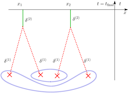
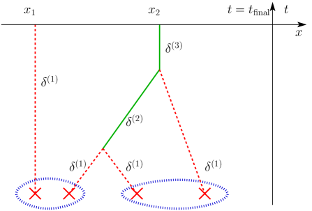
Refer to caption
Refer to caption
Refer to caption
Figure 1: Diagrammatic representation of P22subscript𝑃22P_{22} (top left), P13subscript𝑃13P_{13} (top right), and P13,ccomb2subscript𝑃13subscriptsuperscript𝑐2combP_{13,\;c^{2}_{\rm comb}} (bottom). Continuous green lines represent Green’s functions, red dashed lines represent free fields, and red crosses circled by a dotted blue line represent correlation among free fields.

3.2.3 Cutoff-(in)dependence

Each diagram is dependent on the cutoff ΛΛ\Lambda: P22subscript𝑃22P_{22} and P13subscript𝑃13P_{13} through the smoothed linear power spectrum, while P13,ccomb2subscript𝑃13subscriptsuperscript𝑐2combP_{13,\;c^{2}_{\rm\,comb}} depends on ΛΛ\Lambda through ccomb2subscriptsuperscript𝑐2combc^{2}_{\rm\,comb}, which is ΛΛ\Lambda dependent because it arises from integrating out the short distance fluctuations. The ΛΛ\Lambda dependence of P13subscript𝑃13P_{13} is to be cancelled by P13,ccomb2subscript𝑃13subscriptsuperscript𝑐2combP_{13,\;c^{2}_{\rm\,comb}}, while the one of P22subscript𝑃22P_{22} from the stochastic fluctuations.

Consider the sum of the P13subscript𝑃13P_{13} and P13,ccomb2subscript𝑃13subscriptsuperscript𝑐2combP_{13,\;c^{2}_{\rm\,comb}} terms. In order for this sum to be ΛΛ\Lambda independent, both must have the same k𝑘k-dependence in the relevant regime. By inspection of (57), we see that P13,ccomb2subscript𝑃13subscriptsuperscript𝑐2combP_{13,\;c^{2}_{\rm\,comb}} goes as k2superscript𝑘2k^{2}, which implies that P13subscript𝑃13P_{13} should behave in the same way in this regime. This is in fact the case, as can be readily verified by taking the k0𝑘0k\rightarrow 0 limit of (56). In particular, we can define a ΛΛ\Lambda-independent renormalized parameter ccomb;ren.subscript𝑐combrenc_{\rm\,comb;ren.} defined at a renormalization scale kren.subscript𝑘renk_{\rm ren.} and a ΛΛ\Lambda-dependent counterterm parameter ccomb;ctr.2(Λ)subscriptsuperscript𝑐2combctrΛc^{2}_{\rm\,comb;ctr.}(\Lambda) such that

ccomb2(a,Λ)=ccomb;ren.2(a,kren.)+ccomb;ctr.2(a,Λ).superscriptsubscript𝑐comb2𝑎Λsuperscriptsubscript𝑐combren2𝑎subscript𝑘rensuperscriptsubscript𝑐combctr2𝑎Λc_{\rm\,comb}^{2}(a,\Lambda)=c_{\rm\,comb;ren.}^{2}(a,k_{\rm ren.})+c_{\rm\,comb;ctr.}^{2}(a,\Lambda)\ . (58)

ccomb;ctr.2(a,Λ)subscriptsuperscript𝑐2combctr𝑎Λc^{2}_{\rm\,comb;ctr.}(a,\Lambda) must have the same time and ΛΛ\Lambda-dependence of P13subscript𝑃13P_{13}, while ccomb;ren.(a,kren.)subscript𝑐combren𝑎subscript𝑘renc_{\rm\,comb;ren.}(a,k_{\rm ren.}) is determined by matching to simulations or to observations at a specific k=kren.𝑘subscript𝑘renk=k_{\rm ren.}. The time dependence of ccomb;ren.2(a)subscriptsuperscript𝑐2combren𝑎c^{2}_{\rm\,comb;ren.}(a) could in general be different from the one of ccomb;ctr.2(a,Λ)subscriptsuperscript𝑐2combctr𝑎Λc^{2}_{\rm\,comb;ctr.}(a,\Lambda). However, for the purposes of this paper, we can approximate them to be equal, and we will check this approximation in a forthcoming paper [27]. We can therefore extract the time dependence of ccomb2(a,Λ)subscriptsuperscript𝑐2comb𝑎Λc^{2}_{\rm\,comb}(a,\Lambda) from the k0𝑘0k\rightarrow 0 limit of P13subscript𝑃13P_{13}. We obtain

ccomb;ctr.2(a,Λ)=ccomb;ctr.2(a0,Λ)Dccomb2(a)Dccomb2(a0),superscriptsubscript𝑐combctr2𝑎Λsuperscriptsubscript𝑐combctr2subscript𝑎0Λsubscript𝐷subscriptsuperscript𝑐2comb𝑎subscript𝐷subscriptsuperscript𝑐2combsubscript𝑎0\displaystyle c_{\rm\,comb;ctr.}^{2}(a,\Lambda)=c_{\rm\,comb;ctr.}^{2}(a_{0},\Lambda)\frac{{\cal}D_{c^{2}_{\rm comb}}(a)}{{\cal}D_{c^{2}_{\rm comb}}(a_{0})}\ , (59)

where

Dccomb2(a)=1a[(6304Ωm21(a)+1202Ωm2(a)+52a32(a)D(a)2)\displaystyle{\cal}D_{c^{2}_{\rm comb}}(a)=\frac{1}{a}\left[\left(63\,{\cal H}_{0}^{4}\Omega_{m}^{2}{\cal F}_{1}(a)+12\,{\cal H}_{0}^{2}\Omega_{m}{\cal F}_{2}(a)+52\,a^{3}{\cal H}^{2}(a)D^{\prime}(a)^{2}\right)\right. (60)
4a32(a)D(a)D(a)(2702Ωm3(a)+284(a))].\displaystyle\qquad\qquad\qquad\quad\left.-4\,a^{3}{\cal H}^{2}(a)\frac{D^{\prime}(a)}{D(a)}\left(27\,{\cal H}_{0}^{2}\Omega_{m}{\cal F}_{3}(a)+28\,{\cal F}_{4}(a)\right)\right]\ .

and

1(a)=0a𝑑a~G(a,a~)D(a~)2a~,2(a)=0a𝑑a~G(a,a~)a~2D(a~)22(a~),formulae-sequencesubscript1𝑎superscriptsubscript0𝑎differential-d~𝑎𝐺𝑎~𝑎𝐷superscript~𝑎2~𝑎subscript2𝑎superscriptsubscript0𝑎differential-d~𝑎𝐺𝑎~𝑎superscript~𝑎2superscript𝐷superscript~𝑎2superscript2~𝑎\displaystyle{\cal F}_{1}(a)=\int_{0}^{a}d\tilde{a}\;G(a,\tilde{a})\;\frac{D(\tilde{a})^{2}}{\tilde{a}}\ ,\qquad\qquad{\cal F}_{2}(a)=\int_{0}^{a}d\tilde{a}\;G(a,\tilde{a})\;\tilde{a}^{2}D^{\prime}(\tilde{a})^{2}{\cal H}^{2}(\tilde{a})\ , (61)
3(a)=0a𝑑a~aG(a,a~)D(a~)2a~,4(a)=0a𝑑a~aG(a,a~)a~2D(a~)22(a~).formulae-sequencesubscript3𝑎superscriptsubscript0𝑎differential-d~𝑎subscript𝑎𝐺𝑎~𝑎𝐷superscript~𝑎2~𝑎subscript4𝑎superscriptsubscript0𝑎differential-d~𝑎subscript𝑎𝐺𝑎~𝑎superscript~𝑎2superscript𝐷superscript~𝑎2superscript2~𝑎\displaystyle{\cal F}_{3}(a)=\int_{0}^{a}d\tilde{a}\;{\partial}_{a}G(a,\tilde{a})\;\frac{D(\tilde{a})^{2}}{\tilde{a}}\ ,\quad\qquad{\cal F}_{4}(a)=\int_{0}^{a}d\tilde{a}\;{\partial}_{a}G(a,\tilde{a})\;\tilde{a}^{2}D^{\prime}(\tilde{a})^{2}{\cal H}^{2}(\tilde{a})\ .

A plot of the time dependence of the speed of sound is given in Fig. 2.
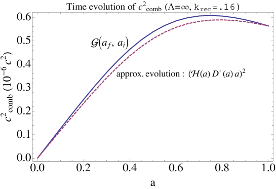
Refer to caption
Figure 2: Time dependence of ccomb2subscriptsuperscript𝑐2combc^{2}_{\rm\,comb} as inferred using the correct time dependence from P13subscript𝑃13P_{13} and instead using the approximate time dependence derived from the growth functions (see App. C). Starting from very early times, we see that ccomb2subscriptsuperscript𝑐2combc^{2}_{\rm\,comb} grows as a functions of time, peaks at about a0.7similar-to-or-equals𝑎0.7a\simeq 0.7, and then decreases near the present epoch, probably as due to the onset of dark energy. ccomb2subscriptsuperscript𝑐2combc^{2}_{\rm\,comb} is positive, implying that this term tends to slow down the collapse of structures.

We determine the value of ccomb;ctr.2(a0,Λ)subscriptsuperscript𝑐2combctrsubscript𝑎0Λc^{2}_{\rm\,comb;ctr.}(a_{0},\Lambda) in two different independent ways: one involving fitting to observation of the power-spectrum derived from simulations, and the other involving direct measurement from simulation. In the first, simplest, way, we determine ccomb;ctr.2(a0,Λ=)subscriptsuperscript𝑐2combctrsubscript𝑎0Λc^{2}_{\rm\,comb;ctr.}(a_{0},\Lambda=\infty) by matching the one-loop EFT power spectrum at k=kren.𝑘subscript𝑘renk=k_{\rm ren.} to the power-spectrum extracted from simulations (or directly from precise observations in the future!). We can do this at various values of ΛΛ\Lambda, but we take the ΛΛ\Lambda\rightarrow\infty limit in order to drive to zero any effect from higher derivative terms down by powers of k/Λ𝑘Λk/\Lambda. At this point, we can derive ccomb2(a0,Λ)subscriptsuperscript𝑐2combsubscript𝑎0Λc^{2}_{\rm\,comb}(a_{0},\Lambda\neq\infty) by running the value at Λ=Λ\Lambda=\infty down to a finite ΛΛ\Lambda. The formula is given by

ccomb2(a0,Λ)=ccomb2(a0,Λ=)+limkext0[(P13(kext,a0,Λ=)P13(kext,a0,Λ))×(2kext2D(a0)0a0da~G(a0,a~)Dccomb2(a~)Dccomb2(a0)D(a~)P11,l(kext,Λ))1].subscriptsuperscript𝑐2combsubscript𝑎0Λsubscriptsuperscript𝑐2combsubscript𝑎0Λsubscriptsubscript𝑘ext0delimited-[]subscript𝑃13subscript𝑘extsubscript𝑎0Λsubscript𝑃13subscript𝑘extsubscript𝑎0Λsuperscript2superscriptsubscript𝑘ext2𝐷subscript𝑎0subscriptsuperscriptsubscript𝑎00𝑑~𝑎𝐺subscript𝑎0~𝑎subscript𝐷subscriptsuperscript𝑐2comb~𝑎subscript𝐷subscriptsuperscript𝑐2combsubscript𝑎0𝐷~𝑎subscript𝑃11𝑙subscript𝑘extΛ1c^{2}_{\rm\,comb}(a_{0},\Lambda\neq\infty)\,=\,c^{2}_{\rm\,comb}(a_{0},\Lambda=\infty)\,+\lim_{k_{\rm ext}\to 0}\Bigg{[}\Big{(}{P_{13}(k_{\rm ext},a_{0},\Lambda=\infty)-P_{13}(k_{\rm ext},a_{0},\Lambda)}\Big{)}\times\\ \left({-2\frac{k_{\rm ext}^{2}}{D(a_{0})}\int^{a_{0}}_{0}d\tilde{a}\;G(a_{0},\tilde{a})\,\frac{{\cal}D_{c^{2}_{\rm comb}}(\tilde{a})}{{\cal}D_{c^{2}_{\rm comb}}(a_{0})}\,D(\tilde{a})\,P_{11,l}(k_{\rm ext},\Lambda)}\right)^{-1}\Bigg{]}\ . (62)

The limit kext0subscript𝑘ext0k_{\rm ext}\to 0 is necessary in order to suppress higher derivative terms down by powers of kext/Λsubscript𝑘extΛk_{\rm ext}/\Lambda. The running of ccomb2subscriptsuperscript𝑐2combc^{2}_{\rm\,comb} is plotted in Fig. 3. ccomb2(a0,Λ=)6.2×10⁷similar-to-or-equalssubscriptsuperscript𝑐2combsubscript𝑎0Λ6.2superscript107c^{2}_{\rm\,comb}(a_{0},\Lambda=\infty)\simeq 6.2\times 10^{-7} and is the value obtained by fitting to data using kren.=0.16hsubscript𝑘ren0.16k_{\rm ren.}=0.16\,h Mpc-1 777It is somewhat interesting to notice that by using csv107similar-tosubscript𝑐𝑠𝑣superscript107c_{sv}\sim 10^{-7} we find a shear viscosity of order η20similar-to𝜂20\eta\sim 20 Pa s, in SI units. This value is very similar to that of some everyday items such as chocolate syrup!. We see that as ΛΛ\Lambda decreases, we integrate out more and more modes, and ccomb2subscriptsuperscript𝑐2combc^{2}_{\rm\,comb} grows. We see that the result matches with the one obtained by the second method for measuring ccomb2subscriptsuperscript𝑐2combc^{2}_{\rm\,comb}, that is by using N𝑁N-body simulation to extract directly the correlations in (30). We perform measurements at Λ=1/3hΛ13\Lambda=1/3\,h Mpc-1 and Λ=1/6hΛ16\Lambda=1/6\,h Mpc-1, and we see that the match is extremely good. We describe more precisely how these measurements are derived in Sec. 4. We take this as an extremely promising indication of the strength of our approach.
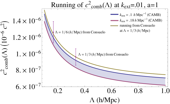
Refer to caption
Figure 3: Running of ccomb2superscriptsubscript𝑐comb2c_{\rm\,comb}^{2} as a function of ΛΛ\Lambda. The purple band contains the region for the values of ccomb2superscriptsubscript𝑐comb2c_{\rm\,comb}^{2} as inferred from matching with the non-linear power spectrum from CAMB at the renormalization scale k=0.1h𝑘0.1k=0.1h Mpc-1 and k=0.18h𝑘0.18k=0.18h Mpc-1. The dependence on the renormalization scale is a measure of the importance of higher loops. We see that as ΛΛ\Lambda\to\infty, ccomb2superscriptsubscript𝑐comb2c_{\rm\,comb}^{2} decreases as more and more modes are included within the regime of validity of the EFT. However, the fact that as Λ=Λ\Lambda=\infty, ccomb20superscriptsubscript𝑐comb20c_{\rm\,comb}^{2}\neq 0 is an indication of the fact that the fundamental theory is not described by a pressureless ideal fluid, but by indeed freely streaming dark matter particles. Data points with 1σ1𝜎1\,\sigma error bars represent the value obtained from N𝑁N-body numerical simulations using the methods described in Sec. 4 using two different smoothing lengths Λ1superscriptΛ1\Lambda^{-1}. Given the error bars from numerical evaluation, the measured values are in remarkable agreement with what inferred from renormalizing using the power spectrum.

In order to elucidate the effect of the higher derivative terms, we plot in Fig. 4 the value of ccomb2(a0,Λ=1/3)subscriptsuperscript𝑐2combsubscript𝑎0Λ13c^{2}_{\rm\,comb}(a_{0},\Lambda=1/3), for various values of the external kextsubscript𝑘extk_{\rm ext}. It is only for vary low kextsubscript𝑘extk_{\rm ext}’s that ccomb2subscriptsuperscript𝑐2combc^{2}_{\rm\,comb} becomes kext.subscript𝑘extk_{\rm ext.} independent.

Refer to caption
Figure 4: In this plot we present to values obtained for ccomb2subscriptsuperscript𝑐2combc^{2}_{\rm\,comb} as a function of the external momentum used in (62). We see that only as kext0subscript𝑘ext0k_{\rm ext}\to 0, ccomb2subscriptsuperscript𝑐2combc^{2}_{\rm\,comb} becomes kextsubscript𝑘extk_{\rm ext} independent. This is so because at high k𝑘k any higher derivative terms suppressed by powers of k/kNL𝑘subscript𝑘𝑁𝐿k/k_{NL} are important.

Finally, there is a third method in which we could have derived ccomb2(a0,Λ)subscriptsuperscript𝑐2combsubscript𝑎0Λc^{2}_{\rm\,comb}(a_{0},\Lambda). By keeping ΛΛ\Lambda finite, we could have fit the analytical results to N𝑁N-body simulations by including higher derivative terms proportional to powers of k/Λ𝑘Λk/\Lambda. Indeed, unless ΛΛ\Lambda\rightarrow\infty, the largest of these terms are not negligible and need to be included to get the correct ccomb2(a0,Λ)subscriptsuperscript𝑐2combsubscript𝑎0Λc^{2}_{\rm\,comb}(a_{0},\Lambda). A description of this approach in detail is given in App. E, and leads to the same results for ccomb2(a0,Λ)subscriptsuperscript𝑐2combsubscript𝑎0Λc^{2}_{\rm\,comb}(a_{0},\Lambda).

4 Fluid parameters from N𝑁N-body simulations

If this language of effective field theory is to be born out, we must be able to take the fundamental theory, integrate away UV effects, and find agreement in terms of the parameters described above. Fortunately we have, in the form of simulation, exactly those calculations in the fundamental theory. By smearing the positions of simulated particles with a normalized Gaussian function of width ΛΛ\Lambda, we are able to introduce a soft UV cutoff of order 1/Λ1Λ1/\Lambda. For correlations on scales longer then the cutoff we can directly measure ccomb2superscriptsubscript𝑐comb2c_{\rm comb}^{2} corroborating the perturbative analysis presented above.

Specifically we consider random downsamples of positions and velocities of the Consuleo simulation888The simulation parameters are: Ωm=0.25subscriptΩ𝑚0.25\Omega_{m}=0.25, ΩΛ=0.75subscriptΩΛ0.75\Omega_{\Lambda}=0.75, h=0.70.7h=0.7 (H=70km/s/Mpc𝐻70kmsMpcH=70~{}{\rm km/s/Mpc}), σ8=0.8subscript𝜎80.8\sigma_{8}=0.8, and ns=1subscript𝑛𝑠1n_{s}=1 with measurements described taking place at z=0𝑧0z=0. [28] from 2.7×1092.7superscript1092.7\times 10^{9} particles downsampled to 1,000,05310000531,000,053 particles distributed over (420Mpc)3superscript420Mpc3(420~{}{\rm Mpc})^{3}. Even this incredibly coarse resolution allows us to measure the following fields δlsubscript𝛿𝑙\delta_{l}, ΘlsubscriptΘ𝑙\Theta_{l}, 2δlsuperscript2subscript𝛿𝑙\partial^{2}\delta_{l}, 2Θlsuperscript2subscriptΘ𝑙\partial^{2}\Theta_{l}, and Assubscript𝐴𝑠A_{s} to measure ccomb2subscriptsuperscript𝑐2comb{c^{2}_{\rm comb}} to within standard errors of 101010 percent. While the complexity of the first four fields go linearly in the number of particles, Assubscript𝐴𝑠A_{s} is more expensive. The fact that we can achieve such consistency with such a small number of particles is not only remarkable, but numerically quite convenient. We describe the details of the analysis in App. D.1, and here simply provide a summary of the results.

The spatial dependence of measured ccomb2subscriptsuperscript𝑐2comb{c^{2}_{\rm comb}} are plotted for Λ=1/3hΛ13\Lambda=1/3\,h Mpc-1 and Λ=1/6hΛ16\Lambda=1/6\,h Mpc-1 in Fig. 5. These regions were chosen to maximize numerical stability as described in App. D. Fitting a constant to the value of ccomb2subscriptsuperscript𝑐2comb{c^{2}_{\rm comb}} for the displayed values after the UV cutoff gives in units of c2superscript𝑐2c^{2}, we obtain

ccomb2(Λ=1/3)subscriptsuperscript𝑐2combΛ13\displaystyle{c^{2}_{\rm comb}}{(\Lambda=1/3)} =0.96±.1×106,absentplus-or-minus0.96.1superscript106\displaystyle=0.96\pm.1\times 10^{-6}\,, (63)
ccomb2(Λ=1/6)subscriptsuperscript𝑐2combΛ16\displaystyle{c^{2}_{\rm comb}}{(\Lambda=1/6)} =1.26±.1×106.absentplus-or-minus1.26.1superscript106\displaystyle=1.26\pm.1\times 10^{-6}\,.
Refer to caption
Refer to caption
Figure 5: Measurement of ccomb2subscriptsuperscript𝑐2comb{c^{2}_{\rm comb}} in the UV with Λ=1/3hΛ13\Lambda=1/3~{}h Mpc-1 and Λ=1/6hΛ16\Lambda=1/6~{}h Mpc-1.

The RG flow between the two measured values is consistent with the prediction from perturbation theory as seen in Fig. 3. Furthermore the measured value from Consuelo agrees nicely with that predicted from matching to the nonlinear CAMB power spectrum.

5 Results

The 𝒪(δl4)𝒪superscriptsubscript𝛿𝑙4{\cal{O}}(\delta_{l}^{4}) result of the computation of the power spectrum with our EFT is presented in Fig. 6. On top, we plot the ratio of the one loop power spectrum compared with the non-linear fit provided by the CAMB software with high precision settings, evaluated with the following cosmological parameters: ΩΛ=0.75,Ωm=0.25,Ωb=0.04,h=0.7,ns=1formulae-sequencesubscriptΩΛ0.75formulae-sequencesubscriptΩ𝑚0.25formulae-sequencesubscriptΩ𝑏0.04formulae-sequence0.7subscript𝑛𝑠1\Omega_{\Lambda}=0.75\;,\Omega_{m}=0.25,\;\Omega_{b}=0.04,\;h=0.7,\;n_{s}=1. The linear power spectrum is also obtained from CAMB with high precision settings. We take these data for all perturbative calculations done in the paper. Often in the literature the results of perturbation theory are plotted as ratio of the perturbation theory result versus a no-wiggle power spectrum. In this way the oscillatory features are still present in the plot, though they come mostly from the linear theory. We give this in the bottom part of the plot.
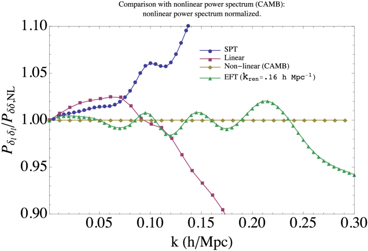
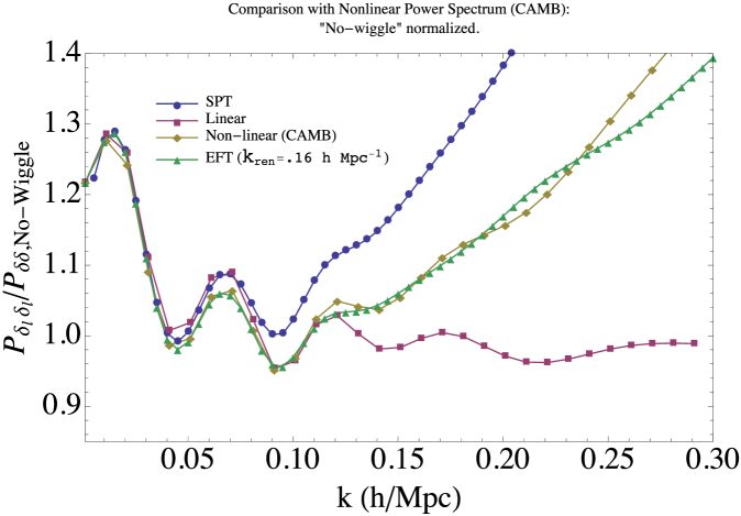
Refer to caption
Refer to caption
Figure 6: The order δl4superscriptsubscript𝛿𝑙4\delta_{l}^{4} prediction from our EFT is compared with the CAMB non-linear output in the top, and to the no-wiggle power spectrum in the bottom, as well with the linear theory and Standard Perturbation Theory (SPT). The results from the EFT agree at percent level with the non-linear theory up to k0.24hsimilar-to-or-equals𝑘0.24k\simeq 0.24h Mpc-1, when some high scale power seems to be missing. Results should improve already by going to δl5superscriptsubscript𝛿𝑙5\delta_{l}^{5} order. The results are remarkably better than using SPT. The no-wiggle power spectrum we use is given by Pδδ,NoWiggle=5.1106qlog2(13q+2e)/(54q2(14+731/(457q+1))+log(13q+2e))2subscript𝑃𝛿𝛿NoWiggle5.1superscript106𝑞superscript213𝑞2𝑒superscript54superscript𝑞214731457𝑞113𝑞2𝑒2P_{\delta\delta,{\rm No-Wiggle}}=5.1\cdot 10^{6}q\log^{2}(13q+2e)/(54\,q^{2}(14+731/(457q+1))+\log(13q+2e))^{2}.

This plot is obtained after renormalizing the EFT prediction to match the power spectrum at kren.=0.16hsubscript𝑘ren0.16k_{\rm ren.}=0.16h\ Mpc-1. In detail, we perform the calculation at several increasing values of ΛΛ\Lambda, we choose the value of ccomb2(a0,Λ)subscriptsuperscript𝑐2combsubscript𝑎0Λc^{2}_{\rm\,comb}(a_{0},\Lambda) to match the simulations’ non-linear output, and then we extrapolate to ΛΛ\Lambda\to\infty. This gives us ccomb2(a0,Λ=)6.2×10⁷similar-to-or-equalssubscriptsuperscript𝑐2combsubscript𝑎0Λ6.2superscript107c^{2}_{\rm\,comb}(a_{0},\Lambda=\infty)\simeq 6.2\times 10^{-7}. Notice that naive considerations of virialization gave an estimated value for ccomb2subscriptsuperscript𝑐2combc^{2}_{\rm\,comb} of order 105superscript10510^{-5} [4]. The obtained smaller numerical value fits well with the decrease in the transfer functions for wavenumbers that are higher than the equality scale.

The result for the power spectrum agrees at percent level with the CAMB non-linear fit up to k0.24hsimilar-to-or-equals𝑘0.24k\simeq 0.24h Mpc-1, where the EFT prediction begins to be smaller than the N𝑁N-body simulation result. Results obtained with the approximate time dependence described in App. C are close to these ones, at percent level. As discussed in App. C, it is potentially dangerous to trust this approximation at high k𝑘k’s for percent level precision, and luckily it is not very hard at all to perform the correct perturbation theory. We expect that the inclusion of the stochastic pressure and of higher order diagrams should improve the fit in the UV, possibly allowing us to fit the simulations to even higher k𝑘k’s. Notice how the counterterm P13,ccomb2subscript𝑃13superscriptsubscript𝑐comb2P_{13,\,c_{\rm comb}^{2}} decreases the power spectrum, compensating for the overshooting of SPT. It is difficult to interpret the percent disagreement that we have at moderate slow scales such as at k0.12hsimilar-to-or-equals𝑘0.12k\simeq 0.12h Mpc-1. At face value, it looks like that the computed power spectrum presents oscillations that are too large. These disagreements might be improved with the inclusion of higher order terms, or it might even be that at this level of precision, the results from the CAMB non-linear fit or from the N𝑁N-body simulations might not be precise enough. These same improvements should reduce also the dependence on the renormalization scale: by changing the renormalization scale our results change by about 2%, at k0.24hsimilar-to𝑘0.24k\sim 0.24h Mpc-1. This dependence can be taken as a measure of the contribution from higher order terms.

6 Conclusions

Large scale structure surveys have the potential of becoming the next leading observational window on the physics of the early universe, potentially greatly improving what we are already learning from the CMB. Large Scale Structure physics is however much more complicated than the CMB due to the presence of large matter clustering at small scales. Since at non-linear level different scales are coupled, these non-linearities affect even large scale perturbations that are mildly non linear and so potentially treatable in a perturbative matter. In this paper we have developed the effective field theory of cosmological large scale structures in order to achieve a reliable predictability. Calculations in the effective theory are performed in k/kNL𝑘subscript𝑘𝑁𝐿k/k_{NL}. The effective field theory is a cosmological fluid description for cold dark matter, and by extension all matter including baryons which trace the dark matter. The microphysical description is in terms of a classical gas of point particles, which we have smoothed at the level of the Boltzmann equation. We have exhibited and computed the various couplings that appear in the effective field theory, namely pressure and viscosity by matching to N𝑁N-body simulations, finding cs2106c2similar-tosuperscriptsubscript𝑐𝑠2superscript106superscript𝑐2c_{s}^{2}\sim 10^{-6}\,c^{2}, etc. . We have developed the perturbative expansion for the power spectrum, which we have carried out at the 𝒪(δl4)𝒪superscriptsubscript𝛿𝑙4{\cal O}(\delta_{l}^{4}). The fluid parameters arise from UV modes and alter standard perturbation theory. We have found that the corrections lead to a power spectrum in percent agreement with the full nonlinear spectrum as obtained by CAMB up to k0.24hsimilar-to-or-equals𝑘0.24k\simeq 0.24h Mpc-1.

It is a peculiar coincidence that k0.24hsimilar-to-or-equals𝑘0.24k\simeq 0.24h Mpc-1 is also the maximum k𝑘k at which the popular technique of Renormalized Perturbation Theory (RPT) [9] works. While RPT is a very nice technique to compute non-linear corrections to the power spectrum, we stress that our approach is different at a qualitative and a quantitative level. At a qualitative level, RPT tries to solve, as exactly as possible, non-linear equations for a pressureless ideal fluid. In our approach, instead, we try to solve non-linear equations for a different fluid. This has quantitative effects, as it is shown from the fact that as ΛΛ\Lambda\to\infty our effective parameters like ccomb2superscriptsubscript𝑐comb2c_{\rm comb}^{2} do not vanish. What is more important about our EFT is that in can be improved. By performing higher order computations and by adding suitable counterterms, in principle arbitrary precision for reconstructing the power spectrum, or indeed any dark matter observables, can be achieved by going to a sufficiently high order in perturbation theory, on scales kkNLless-than-or-similar-to𝑘subscript𝑘𝑁𝐿k\lesssim k_{NL}. Techniques such as RPT or the renormalization group approach [15] for example are still very nice techniques to perturbatively solve some non-linear equations, resumming many diagrams. It would be interesting to apply those techniques to solve the equations of our EFT. We leave this to future work.

The effective field theory approach to large scale structure formation is complimentary to N𝑁N-body simulations by providing an elegant fluid description. This provides intuition for various nonlinear effects, as well as providing computational efficiency, since the numerics required to measure the fluid parameters are expected to be computationally less expensive than a full scale simulation. Indeed we are able to achieve excellent agreement with the small down-sample of the full simulation we examined here. Of course, since the couplings are UV sensitive, it still requires the use of some form of N𝑁N-body simulation to fix the physical parameters, either by matching to the stress-tensor directly or to observables. But this matching is only for a small number of physical parameters at some scale and then the constructed field theory is predictive at other scales.

There are several possible extensions of this work. A first extension is to go beyond the one-loop order to two-loop, or higher. This will require the measurement of several new parameters that will enter the effective stress-tensor at higher order, including its stochastic terms. Another extension is to compute the velocity fields and to include the small but finite contributions from vorticity, or to compute higher order N𝑁N-point functions, which can probe non-Gaussianity. Finally, another extension is to consider different cosmologies; in this work we have presented results on dark energy in the form of a cosmological constant. But one could equally consider other models for dark energy. This would presumably alter the value of the fluid parameters in a way that could be measured either from new simulations or determined by observation. Hopefully, our effective field theory for large scale structures will help us use large scale structure surveys to uncover the physics of the beginning of the universe.

Acknowledgments

We thank T. Abel, A. Arvanitaki, T. Baldauf, D. Baumann, P. Behroozi, S. Dubovsky, S. Foreman, S. Kachru, A. Nicolis, U. Seljak, G. Villadoro, R. Wechsler and M. Zaldarriaga for many useful conversations. We gratefully acknowledge Academic Technology Services at UCLA for computer support. We are also thankful to M. Busha and R. Wechsler for providing us with data on the dark matter distribution from the Consuelo simulation, which was run using the orange cluster at SLAC by M. Busha as part of the LASDAMAS project. J.J.M.C. is supported by the Stanford Institute for Theoretical Physics and the NSF grant no. PHY-0756174. M.P.H. is supported by NSF grant PHY-0756174 and a Kavli Fellowship. L.S. is supported by DOE Early Career Award DE-FG02-12ER41854 and by NSF grant PHY-1068380.

Appendix

Appendix A UV Stress Tensor directly from Short Modes

It is useful to write down the expression (22) directly in terms of short wavelength fluctuations. In this Appendix we provide these expressions. We define

σsijsuperscriptsubscript𝜎𝑠𝑖𝑗\displaystyle\sigma_{s}^{ij} \displaystyle\!\!\equiv m1a5d3𝐩(pipli(𝐱))(pjplj(𝐱))f(𝐱,𝐩)superscript𝑚1superscript𝑎5superscript𝑑3𝐩superscript𝑝𝑖subscriptsuperscript𝑝𝑖𝑙𝐱superscript𝑝𝑗subscriptsuperscript𝑝𝑗𝑙𝐱𝑓𝐱𝐩\displaystyle\!\!m^{-1}a^{-5}\!\int\!d^{3}{\bf p}\,(p^{i}-p^{i}_{l}({\bf x}))(p^{j}-p^{j}_{l}({\bf x}))f({\bf x},{\bf p}) (64)
=\displaystyle\!\!= nma3(vnivli(𝐱n))(vnjvlj(𝐱n))δD(3)(𝐱𝐱n),subscript𝑛𝑚superscript𝑎3superscriptsubscript𝑣𝑛𝑖superscriptsubscript𝑣𝑙𝑖subscript𝐱𝑛superscriptsubscript𝑣𝑛𝑗superscriptsubscript𝑣𝑙𝑗subscript𝐱𝑛subscriptsuperscript𝛿3𝐷𝐱subscript𝐱𝑛\displaystyle\!\!\sum_{n}{m\over a^{3}}(v_{n}^{i}-v_{l}^{i}({\bf x}_{n}))(v_{n}^{j}-v_{l}^{j}({\bf x}_{n}))\,\delta^{(3)}_{D}({\bf x}-{\bf x}_{n})\ ,\,\,\,\,\,\,\,\,\,\,\, (65)
ϕs,nsubscriptitalic-ϕ𝑠𝑛\displaystyle\phi_{s,n} \displaystyle\!\!\equiv ϕnϕl,n,subscriptitalic-ϕ𝑛subscriptitalic-ϕ𝑙𝑛\displaystyle\!\!\phi_{n}-\phi_{l,n}\ , (66)
iϕssubscript𝑖subscriptitalic-ϕ𝑠\displaystyle\partial_{i}\phi_{s} =\displaystyle\!\!= niϕs,n,subscript𝑛subscript𝑖subscriptitalic-ϕ𝑠𝑛\displaystyle\!\!\sum_{n}\partial_{i}\phi_{s,n}\ , (67)
wsijsubscriptsuperscript𝑤𝑖𝑗𝑠\displaystyle w^{ij}_{s} \displaystyle\!\!\equiv iϕsjϕsniϕs,njϕs,n,subscript𝑖subscriptitalic-ϕ𝑠subscript𝑗subscriptitalic-ϕ𝑠subscript𝑛subscript𝑖subscriptitalic-ϕ𝑠𝑛subscript𝑗subscriptitalic-ϕ𝑠𝑛\displaystyle\!\!\partial_{i}\phi_{s}\,\partial_{j}\phi_{s}-\sum_{n}\partial_{i}\phi_{s,n}\,\partial_{j}\phi_{s,n}\ , (68)

where pli(𝐱)mavli(𝐱)superscriptsubscript𝑝𝑙𝑖𝐱𝑚𝑎superscriptsubscript𝑣𝑙𝑖𝐱p_{l}^{i}({\bf x})\equiv m\,a\,v_{l}^{i}({\bf x}). Note that σsijσijσlijsubscriptsuperscript𝜎𝑖𝑗𝑠superscript𝜎𝑖𝑗superscriptsubscript𝜎𝑙𝑖𝑗\sigma^{ij}_{s}\neq\sigma^{ij}-\sigma_{l}^{ij}, but they are related as follows

σlijsuperscriptsubscript𝜎𝑙𝑖𝑗\displaystyle\sigma_{l}^{ij} =\displaystyle\!\!= [σsij]Λ+[ρmvlivlj]Λ+[vli(πjρmvlj)+vlj(πiρmvli)]Λ.subscriptdelimited-[]superscriptsubscript𝜎𝑠𝑖𝑗Λsubscriptdelimited-[]subscript𝜌𝑚superscriptsubscript𝑣𝑙𝑖superscriptsubscript𝑣𝑙𝑗Λsubscriptdelimited-[]superscriptsubscript𝑣𝑙𝑖superscript𝜋𝑗subscript𝜌𝑚superscriptsubscript𝑣𝑙𝑗superscriptsubscript𝑣𝑙𝑗superscript𝜋𝑖subscript𝜌𝑚superscriptsubscript𝑣𝑙𝑖Λ\displaystyle\!\!\left[\sigma_{s}^{ij}\right]_{\Lambda}+\left[\rho_{m}v_{l}^{i}v_{l}^{j}\right]_{\Lambda}+\left[v_{l}^{i}(\pi^{j}-\rho_{m}v_{l}^{j})+v_{l}^{j}(\pi^{i}-\rho_{m}v_{l}^{i})\right]_{\Lambda}\ . (69)

The second term is approximately ρlvlivljsubscript𝜌𝑙superscriptsubscript𝑣𝑙𝑖superscriptsubscript𝑣𝑙𝑗\rho_{l}v_{l}^{i}v_{l}^{j} (so it approximately cancels with ρlvlivljsubscript𝜌𝑙superscriptsubscript𝑣𝑙𝑖superscriptsubscript𝑣𝑙𝑗-\rho_{l}v_{l}^{i}v_{l}^{j} in κlijsuperscriptsubscript𝜅𝑙𝑖𝑗\kappa_{l}^{ij}) and the final term is small (as it is an overlap between short and long modes). Following the methods of [4] we obtain

κlij=[σsij]Λ+ρlkvlikvljΛ2+𝒪(1Λ4).superscriptsubscript𝜅𝑙𝑖𝑗subscriptdelimited-[]superscriptsubscript𝜎𝑠𝑖𝑗Λsubscript𝜌𝑙subscript𝑘superscriptsubscript𝑣𝑙𝑖subscript𝑘superscriptsubscript𝑣𝑙𝑗superscriptΛ2𝒪1superscriptΛ4\displaystyle\kappa_{l}^{ij}=\left[\sigma_{s}^{ij}\right]_{\Lambda}+{\rho_{l}\partial_{k}v_{l}^{i}\partial_{k}v_{l}^{j}\over\Lambda^{2}}+\mathcal{O}\left(1\over\Lambda^{4}\right)\ . (70)

Similarly, one can prove that ΦlijsubscriptsuperscriptΦ𝑖𝑗𝑙\Phi^{ij}_{l} satisfies

ΦlijsubscriptsuperscriptΦ𝑖𝑗𝑙\displaystyle\Phi^{ij}_{l} =\displaystyle\!\!= [wskk]Λδij2[wsij]Λ8πGa2+limit-fromsubscriptdelimited-[]subscriptsuperscript𝑤𝑘𝑘𝑠Λsuperscript𝛿𝑖𝑗2subscriptdelimited-[]subscriptsuperscript𝑤𝑖𝑗𝑠Λ8𝜋𝐺superscript𝑎2\displaystyle\!\!-{[w^{kk}_{s}]_{\Lambda}\delta^{ij}-2[w^{ij}_{s}]_{\Lambda}\over 8\pi G\,a^{2}}+ (71)
mkϕlmkϕlδij2miϕlmjϕl8πGa2Λ2+𝒪(1Λ4).subscript𝑚subscript𝑘subscriptitalic-ϕ𝑙subscript𝑚subscript𝑘subscriptitalic-ϕ𝑙superscript𝛿𝑖𝑗2subscript𝑚subscript𝑖subscriptitalic-ϕ𝑙subscript𝑚subscript𝑗subscriptitalic-ϕ𝑙8𝜋𝐺superscript𝑎2superscriptΛ2𝒪1superscriptΛ4\displaystyle\!\!\!\!\!\!\!{\partial_{m}\partial_{k}\phi_{l}\partial_{m}\partial_{k}\phi_{l}\delta^{ij}-2\partial_{m}\partial_{i}\phi_{l}\partial_{m}\partial_{j}\phi_{l}\over 8\pi G\,a^{2}\Lambda^{2}}+\mathcal{O}\!\left(1\over\Lambda^{4}\right)\ .\,\,\,\,\,\,\,\,\,\,

So altogether we obtain the effective stress-tensor

[τij]Λsubscriptdelimited-[]superscript𝜏𝑖𝑗Λ\displaystyle\left[\tau^{ij}\right]_{\Lambda} =\displaystyle\!\!= [τsij]Λ+[τij]2,subscriptdelimited-[]superscriptsubscript𝜏𝑠𝑖𝑗Λsuperscriptdelimited-[]superscript𝜏𝑖𝑗superscript2\displaystyle\!\!\left[\tau_{s}^{ij}\right]_{\Lambda}+\left[\tau^{ij}\right]^{\partial^{2}}\ , (72)

where

[τsij]Λsubscriptdelimited-[]superscriptsubscript𝜏𝑠𝑖𝑗Λ\displaystyle\left[\tau_{s}^{ij}\right]_{\Lambda} =\displaystyle\!\!= [σsij]Λ[wskk]Λδij2[wsij]Λ8πGa2,subscriptdelimited-[]superscriptsubscript𝜎𝑠𝑖𝑗Λsubscriptdelimited-[]subscriptsuperscript𝑤𝑘𝑘𝑠Λsuperscript𝛿𝑖𝑗2subscriptdelimited-[]subscriptsuperscript𝑤𝑖𝑗𝑠Λ8𝜋𝐺superscript𝑎2\displaystyle\!\!\left[\sigma_{s}^{ij}\right]_{\Lambda}-{[w^{kk}_{s}]_{\Lambda}\delta^{ij}-2[w^{ij}_{s}]_{\Lambda}\over 8\pi G\,a^{2}}\ , (73)
[τij]2superscriptdelimited-[]superscript𝜏𝑖𝑗superscript2\displaystyle\left[\tau^{ij}\right]^{\partial^{2}} =\displaystyle\!\!= ρlkvlikvljΛ2+mkϕlmkϕlδij2miϕlmjϕl8πGa2Λ2+𝒪(1Λ4).subscript𝜌𝑙subscript𝑘superscriptsubscript𝑣𝑙𝑖subscript𝑘superscriptsubscript𝑣𝑙𝑗superscriptΛ2subscript𝑚subscript𝑘subscriptitalic-ϕ𝑙subscript𝑚subscript𝑘subscriptitalic-ϕ𝑙superscript𝛿𝑖𝑗2subscript𝑚subscript𝑖subscriptitalic-ϕ𝑙subscript𝑚subscript𝑗subscriptitalic-ϕ𝑙8𝜋𝐺superscript𝑎2superscriptΛ2𝒪1superscriptΛ4\displaystyle\!\!{\rho_{l}\partial_{k}v_{l}^{i}\partial_{k}v_{l}^{j}\over\Lambda^{2}}+{\partial_{m}\partial_{k}\phi_{l}\partial_{m}\partial_{k}\phi_{l}\delta^{ij}-2\partial_{m}\partial_{i}\phi_{l}\partial_{m}\partial_{j}\phi_{l}\over 8\pi G\,a^{2}\Lambda^{2}}+\mathcal{O}\!\left(1\over\Lambda^{4}\right)\ .\,\,\,\,\,\,\,\,\,\, (74)

We see that [τij]Λsubscriptdelimited-[]superscript𝜏𝑖𝑗Λ[\tau^{ij}]_{\Lambda} is sourced by short wavelength fluctuations plus higher derivative corrections.

Note that by taking the derivative jsubscript𝑗\partial_{j} this leading piece becomes

j[τsij]Λ=j[σsij]Λ+[ρsiϕs]Λ,subscript𝑗subscriptdelimited-[]subscriptsuperscript𝜏𝑖𝑗𝑠Λsubscript𝑗subscriptdelimited-[]superscriptsubscript𝜎𝑠𝑖𝑗Λsubscriptdelimited-[]subscript𝜌𝑠subscript𝑖subscriptitalic-ϕ𝑠Λ\displaystyle\partial_{j}[\tau^{ij}_{s}]_{\Lambda}=\partial_{j}\!\left[\sigma_{s}^{ij}\right]_{\Lambda}+\left[\rho_{s}\partial_{i}\phi_{s}\right]_{\Lambda}\ , (75)

with

[ρsiϕs]Λ=nn¯ma3iϕs,n¯(𝐱n)WΛ(𝐱𝐱n)[ρliϕs]Λ,subscriptdelimited-[]subscript𝜌𝑠subscript𝑖subscriptitalic-ϕ𝑠Λsubscript𝑛¯𝑛𝑚superscript𝑎3subscript𝑖subscriptitalic-ϕ𝑠¯𝑛subscript𝐱𝑛subscript𝑊Λ𝐱subscript𝐱𝑛subscriptdelimited-[]subscript𝜌𝑙subscript𝑖subscriptitalic-ϕ𝑠Λ[\rho_{s}\partial_{i}\phi_{s}]_{\Lambda}=\sum_{n\neq\bar{n}}m\,a^{-3}\partial_{i}\phi_{s,\bar{n}}({\bf x}_{n})W_{\Lambda}({\bf x}-{\bf x}_{n})-[\rho_{l}\partial_{i}\phi_{s}]_{\Lambda}\ , (76)

where the first term in (76) is given by

nn¯ma3iϕs,n¯(𝐱n)WΛ(𝐱𝐱n)subscript𝑛¯𝑛𝑚superscript𝑎3subscript𝑖subscriptitalic-ϕ𝑠¯𝑛subscript𝐱𝑛subscript𝑊Λ𝐱subscript𝐱𝑛\displaystyle\sum_{n\neq\bar{n}}m\,a^{-3}\partial_{i}\phi_{s,\bar{n}}({\bf x}_{n})W_{\Lambda}({\bf x}-{\bf x}_{n})
=nn¯m2Ga4(xnxn¯)i|𝐱n𝐱n¯|3(Erfc[Λ|𝐱n𝐱n¯|2]+4π|𝐱n𝐱n¯|Λ2WΛ(𝐱n𝐱n¯))WΛ(𝐱𝐱n),absentsubscript𝑛¯𝑛superscript𝑚2𝐺superscript𝑎4superscriptsubscript𝑥𝑛subscript𝑥¯𝑛𝑖superscriptsubscript𝐱𝑛subscript𝐱¯𝑛3Erfcdelimited-[]Λsubscript𝐱𝑛subscript𝐱¯𝑛24𝜋subscript𝐱𝑛subscript𝐱¯𝑛superscriptΛ2subscript𝑊Λsubscript𝐱𝑛subscript𝐱¯𝑛subscript𝑊Λ𝐱subscript𝐱𝑛\displaystyle=\sum_{n\neq\bar{n}}{m^{2}G\over a^{4}}{(x_{n}-x_{\bar{n}})^{i}\over|{\bf x}_{n}-{\bf x}_{\bar{n}}|^{3}}\left(\mbox{Erfc}\left[{\Lambda|{\bf x}_{n}-{\bf x}_{\bar{n}}|\over\sqrt{2}}\right]+{4\pi|{\bf x}_{n}-{\bf x}_{\bar{n}}|\over\Lambda^{2}}W_{\Lambda}({\bf x}_{n}-{\bf x}_{\bar{n}})\right)W_{\Lambda}({\bf x}-{\bf x}_{n})\ ,\,\,\,\,\,\,\,\,\,\,\,\,\,\,\, (77)

and the second term in (76) can be expanded as

[ρliϕs]Λ=12Λ2ρli2ϕl+,subscriptdelimited-[]subscript𝜌𝑙subscript𝑖subscriptitalic-ϕ𝑠Λ12superscriptΛ2subscript𝜌𝑙subscript𝑖superscript2subscriptitalic-ϕ𝑙[\rho_{l}\partial_{i}\phi_{s}]_{\Lambda}=-{1\over 2\Lambda^{2}}\rho_{l}\partial_{i}\partial^{2}\phi_{l}+\ldots\ , (78)

and this term should be included since it involves the background piece ρbsubscript𝜌𝑏\rho_{b}, and so it includes a first order contribution.

Appendix B Expression for δ(3)superscript𝛿3\delta^{(3)}

The iterative solution for δ(3)superscript𝛿3\delta^{(3)} is given by

δl(3)(k,a)=1256π6D(a0)3subscriptsuperscript𝛿3𝑙𝑘𝑎1256superscript𝜋6𝐷superscriptsubscript𝑎03\displaystyle\delta^{(3)}_{l}(\vec{k},a)=\frac{1}{256\pi^{6}D(a_{0})^{3}} (79)
[4𝒟1(a)(d3qd3pβ(p,qp)δs1(qp)δs1(p)β(q,kq)δs1(kq)\displaystyle\left[4{\cal D}_{1}(a)\left(\int d^{3}q\int d^{3}p\beta(\vec{p},\vec{q}-\vec{p})\delta s_{1}(\vec{q}-\vec{p})\delta s_{1}(\vec{p})\beta(\vec{q},\vec{k}-\vec{q})\delta s_{1}(\vec{k}-\vec{q})\right.\right.
d3qd3pβ(p,kqp)δs1(kqp)δs1(p)β(q,kq)δs1(q))+\displaystyle\ \ \qquad\left.\int d^{3}q\int d^{3}p\beta(\vec{p},\vec{k}-\vec{q}-\vec{p})\delta s_{1}(\vec{k}-\vec{q}-\vec{p})\delta s_{1}(\vec{p})\beta(\vec{q},\vec{k}-\vec{q})\delta s_{1}(\vec{q})\right)+
2𝒟2(a)d3qd3pβ(p,kqp)δs1(kqp)δs1(p)α(q,kq)δs1(q)+limit-from2subscript𝒟2𝑎superscript𝑑3𝑞superscript𝑑3𝑝𝛽𝑝𝑘𝑞𝑝𝛿subscript𝑠1𝑘𝑞𝑝𝛿subscript𝑠1𝑝𝛼𝑞𝑘𝑞𝛿subscript𝑠1𝑞\displaystyle 2{\cal D}_{2}(a)\int d^{3}q\int d^{3}p\beta(\vec{p},\vec{k}-\vec{q}-\vec{p})\delta s_{1}(\vec{k}-\vec{q}-\vec{p})\delta s_{1}(\vec{p})\alpha(\vec{q},\vec{k}-\vec{q})\delta s_{1}(\vec{q})+
𝒟3(a)d3qd3pα(p,kqp)δs1(kqp)δs1(p)α(q,kq)δs1(q)+limit-fromsubscript𝒟3𝑎superscript𝑑3𝑞superscript𝑑3𝑝𝛼𝑝𝑘𝑞𝑝𝛿subscript𝑠1𝑘𝑞𝑝𝛿subscript𝑠1𝑝𝛼𝑞𝑘𝑞𝛿subscript𝑠1𝑞\displaystyle{\cal D}_{3}(a)\int d^{3}q\int d^{3}p\alpha(\vec{p},\vec{k}-\vec{q}-\vec{p})\delta s_{1}(\vec{k}-\vec{q}-\vec{p})\delta s_{1}(\vec{p})\alpha(\vec{q},\vec{k}-\vec{q})\delta s_{1}(\vec{q})+
𝒟4(a)d3qd3pα(p,qp)δs1(qp)δs1(p)α(q,kq)δs1(kq)+limit-fromsubscript𝒟4𝑎superscript𝑑3𝑞superscript𝑑3𝑝𝛼𝑝𝑞𝑝𝛿subscript𝑠1𝑞𝑝𝛿subscript𝑠1𝑝𝛼𝑞𝑘𝑞𝛿subscript𝑠1𝑘𝑞\displaystyle{\cal D}_{4}(a)\int d^{3}q\int d^{3}p\alpha(\vec{p},\vec{q}-\vec{p})\delta s_{1}(\vec{q}-\vec{p})\delta s_{1}(\vec{p})\alpha(\vec{q},\vec{k}-\vec{q})\delta s_{1}(\vec{k}-\vec{q})+
2𝒟5(a)(d3qd3pα(p,qp)δs1(qp)δs1(p)β(q,kq)δs1(kq)\displaystyle 2{\cal D}_{5}(a)\left(\int d^{3}q\int d^{3}p\alpha(\vec{p},\vec{q}-\vec{p})\delta s_{1}(\vec{q}-\vec{p})\delta s_{1}(\vec{p})\beta(\vec{q},\vec{k}-\vec{q})\delta s_{1}(\vec{k}-\vec{q})\right.
d3qd3pα(p,kqp)δs1(kqp)δs1(p)β(q,kq)δs1(q))+\displaystyle\ \ \qquad\left.\int d^{3}q\int d^{3}p\alpha(\vec{p},\vec{k}-\vec{q}-\vec{p})\delta s_{1}(\vec{k}-\vec{q}-\vec{p})\delta s_{1}(\vec{p})\beta(\vec{q},\vec{k}-\vec{q})\delta s_{1}(\vec{q})\right)+
2𝒟6(a)d3qd3pβ(p,qp)δs1(qp)δs1(p)α(q,kq)δs1(kq)],\displaystyle\left.2{\cal D}_{6}(a)\int d^{3}q\int d^{3}p\beta(\vec{p},\vec{q}-\vec{p})\delta s_{1}(\vec{q}-\vec{p})\delta s_{1}(\vec{p})\alpha(\vec{q},\vec{k}-\vec{q})\delta s_{1}(\vec{k}-\vec{q})\right]\ ,

where 𝒟isubscript𝒟𝑖{\cal D}_{i}’s represent the result of the integration of the Green’s functions and the other time-dependent coefficients. They are given by

𝒟1=0a𝑑a~a~2G(a,a~)2(a~)D(a~)0a~𝑑a^a^22(a^)a~G(a~,a^)D(a^)2,subscript𝒟1superscriptsubscript0𝑎differential-d~𝑎superscript~𝑎2𝐺𝑎~𝑎superscript2~𝑎superscript𝐷~𝑎superscriptsubscript0~𝑎differential-d^𝑎superscript^𝑎2superscript2^𝑎subscript~𝑎𝐺~𝑎^𝑎superscript𝐷superscript^𝑎2\displaystyle{\cal D}_{1}=\int_{0}^{a}d\tilde{a}\;\tilde{a}^{2}\,G(a,\tilde{a}){\cal H}^{2}(\tilde{a})D^{\prime}(\tilde{a})\int_{0}^{\tilde{a}}d\hat{a}\;\hat{a}^{2}{\cal H}^{2}(\hat{a}){\partial}_{\tilde{a}}G(\tilde{a},\hat{a})D^{\prime}(\hat{a})^{2}\ , (80)
𝒟2=302Ωm0a𝑑a~G(a,a~)a~0a~𝑑a^a^22(a^)D(a^)2D(a~)G(a~,a^)+2𝒟1,subscript𝒟23superscriptsubscript02subscriptΩ𝑚superscriptsubscript0𝑎differential-d~𝑎𝐺𝑎~𝑎~𝑎superscriptsubscript0~𝑎differential-d^𝑎superscript^𝑎2superscript2^𝑎superscript𝐷superscript^𝑎2𝐷~𝑎𝐺~𝑎^𝑎2subscript𝒟1\displaystyle{\cal D}_{2}=3{\cal H}_{0}^{2}\Omega_{m}\int_{0}^{a}d\tilde{a}\;\frac{G(a,\tilde{a})}{\tilde{a}}\int_{0}^{\tilde{a}}d\hat{a}\;\hat{a}^{2}{\cal H}^{2}(\hat{a})D^{\prime}(\hat{a})^{2}D(\tilde{a})\,G(\tilde{a},\hat{a})+2{\cal D}_{1}\ ,
𝒟3=0a𝑑a~G(a,a~)a~subscript𝒟3superscriptsubscript0𝑎differential-d~𝑎𝐺𝑎~𝑎~𝑎\displaystyle{\cal D}_{3}=\int_{0}^{a}d\tilde{a}\;\frac{G(a,\tilde{a})}{\tilde{a}}
0a~𝑑a^1a^[302ΩmD(a^)2+2a^32(a^)D(a^)2][302ΩmD(a~)G(a~,a^)+2a~32(a~)D(a~)a~G(a~,a^)],superscriptsubscript0~𝑎differential-d^𝑎1^𝑎delimited-[]3superscriptsubscript02subscriptΩ𝑚𝐷superscript^𝑎22superscript^𝑎3superscript2^𝑎superscript𝐷superscript^𝑎2delimited-[]3superscriptsubscript02subscriptΩ𝑚𝐷~𝑎𝐺~𝑎^𝑎2superscript~𝑎3superscript2~𝑎superscript𝐷~𝑎subscript~𝑎𝐺~𝑎^𝑎\displaystyle\ \int_{0}^{\tilde{a}}d\hat{a}\;\frac{1}{\hat{a}}\left[3{\cal H}_{0}^{2}\Omega_{m}D(\hat{a})^{2}+2\hat{a}^{3}{\cal H}^{2}(\hat{a})D^{\prime}(\hat{a})^{2}\right]\left[3{\cal H}_{0}^{2}\Omega_{m}D(\tilde{a})G(\tilde{a},\hat{a})+2\tilde{a}^{3}{\cal H}^{2}(\tilde{a})D^{\prime}(\tilde{a}){\partial}_{\tilde{a}}G(\tilde{a},\hat{a})\right],
𝒟4=𝒟340a𝑑a~a~2G(a,a~)2(a~)D(a~)D(a~)2,subscript𝒟4subscript𝒟34superscriptsubscript0𝑎differential-d~𝑎superscript~𝑎2𝐺𝑎~𝑎superscript2~𝑎𝐷~𝑎superscript𝐷superscript~𝑎2\displaystyle{\cal D}_{4}={\cal D}_{3}-4\int_{0}^{a}d\tilde{a}\;\tilde{a}^{2}\,G(a,\tilde{a}){\cal H}^{2}(\tilde{a})D(\tilde{a})D^{\prime}(\tilde{a})^{2}\ ,
𝒟5=302Ωm0a𝑑a~a~2G(a,a~)2(a~)D(a~)0a~𝑑a^D(a^)2a~G(a~,a^)a^subscript𝒟53superscriptsubscript02subscriptΩ𝑚superscriptsubscript0𝑎differential-d~𝑎superscript~𝑎2𝐺𝑎~𝑎superscript2~𝑎superscript𝐷~𝑎superscriptsubscript0~𝑎differential-d^𝑎𝐷superscript^𝑎2subscript~𝑎𝐺~𝑎^𝑎^𝑎\displaystyle{\cal D}_{5}=3{\cal H}_{0}^{2}\Omega_{m}\int_{0}^{a}d\tilde{a}\;\tilde{a}^{2}\,G(a,\tilde{a})\;{\cal H}^{2}(\tilde{a})D^{\prime}(\tilde{a})\int_{0}^{\tilde{a}}d\hat{a}\;D(\hat{a})^{2}\frac{{\partial}_{\tilde{a}}G(\tilde{a},\hat{a})}{\hat{a}}
20a𝑑a~a~2G(a,a~)2(a~)D(a~)D(a~)2+2𝒟1,2superscriptsubscript0𝑎differential-d~𝑎superscript~𝑎2𝐺𝑎~𝑎superscript2~𝑎𝐷~𝑎superscript𝐷superscript~𝑎22subscript𝒟1\displaystyle\qquad\quad-2\int_{0}^{a}d\tilde{a}\;\tilde{a}^{2}\,G(a,\tilde{a}){\cal H}^{2}(\tilde{a})D(\tilde{a})D^{\prime}(\tilde{a})^{2}+2{\cal D}_{1}\ ,
𝒟6=𝒟2+20a𝑑a~a~2G(a,a~)2(a~)D(a~)D(a~)2.subscript𝒟6subscript𝒟22superscriptsubscript0𝑎differential-d~𝑎superscript~𝑎2𝐺𝑎~𝑎superscript2~𝑎𝐷~𝑎superscript𝐷superscript~𝑎2\displaystyle{\cal D}_{6}={\cal D}_{2}+2\int_{0}^{a}d\tilde{a}\;\tilde{a}^{2}\,G(a,\tilde{a}){\cal H}^{2}(\tilde{a})D(\tilde{a})D^{\prime}(\tilde{a})^{2}\ .

Notice again the great simplification that occurs due to the fact that the growth factors and the Green’s function do not depend on k𝑘k, so that the time integrals and the momentum integrals decouple.

Appendix C 𝒪(δl4)𝒪superscriptsubscript𝛿𝑙4{\cal O}(\delta_{l}^{4}) Power Spectrum with Approximate Treatment

In the main part of the paper, we performed perturbation theory with our EFT in a rigorous and exact way. However, it is possible to perform an approximate treatment that simplifies quite a bit the formulas. In this way it is simpler to follow the derivation and we therefore present it here.

If the universe were to be EdS, then the solution for δ(n)superscript𝛿𝑛\delta^{(n)} would be δ(n)anD(a)nproportional-tosuperscript𝛿𝑛superscript𝑎𝑛similar-to-or-equals𝐷superscript𝑎𝑛\delta^{(n)}\propto a^{n}\simeq D(a)^{n}. Thanks to this, all formulas simplify remarkably. Our universe is of course not of the EdS form, because of the cosmological constant. But it is tempting to extend the results obtained in EdS to the ones in ΛΛ\LambdaCDM universe by replacing in the EdS formulas the EdS growth factor with the growth factor in ΛΛ\LambdaCDM. In this we obtain

δl(k,a0)δl(q,a0)1loop(2π)3δ(3)(k+q)(P~22(k)+P~13(k)+P~13,ccomb2(k)).similar-to-or-equalssubscriptdelimited-⟨⟩subscript𝛿𝑙𝑘subscript𝑎0subscript𝛿𝑙𝑞subscript𝑎01loopsuperscript2𝜋3superscript𝛿3𝑘𝑞subscript~𝑃22𝑘subscript~𝑃13𝑘subscript~𝑃13subscriptsuperscript𝑐2comb𝑘\langle\delta_{l}(\vec{k},a_{0})\delta_{l}(\vec{q},a_{0})\rangle_{\rm 1-loop}\simeq(2\pi)^{3}\delta^{(3)}(\vec{k}+\vec{q})\left(\tilde{P}_{22}(k)+\tilde{P}_{13}(k)+\tilde{P}_{13,\;c^{2}_{\rm\,comb}}(k)\right)\ . (81)

Here P~22subscript~𝑃22\tilde{P}_{22} and P~13subscript~𝑃13\tilde{P}_{13} are the time-independent one loop contributions given by

P~22(k)=k3392π20𝑑r11𝑑x(10rx2+3r+7x)2(r22rx+1)2P11,l(kr,Λ)P11,l(kr22rx+1,Λ),subscript~𝑃22𝑘superscript𝑘3392superscript𝜋2superscriptsubscript0differential-d𝑟superscriptsubscript11differential-d𝑥superscript10𝑟superscript𝑥23𝑟7𝑥2superscriptsuperscript𝑟22𝑟𝑥12subscript𝑃11𝑙𝑘𝑟Λsubscript𝑃11𝑙𝑘superscript𝑟22𝑟𝑥1Λ\displaystyle\tilde{P}_{22}(k)=\frac{k^{3}}{392\pi^{2}}\int_{0}^{\infty}dr\int_{-1}^{1}dx\frac{\left(-10rx^{2}+3r+7x\right)^{2}}{\left(r^{2}-2rx+1\right)^{2}}P_{11,l}(kr,\Lambda)P_{11,l}(k\sqrt{r^{2}-2rx+1},\Lambda)\ ,
P~13(k)=k31008π2P11,l(k,Λ)subscript~𝑃13𝑘superscript𝑘31008superscript𝜋2subscript𝑃11𝑙𝑘Λ\displaystyle\tilde{P}_{13}(k)=\frac{k^{3}}{1008\pi^{2}}P_{11,l}(k,\Lambda) (82)
0𝑑r(3r3(r21)3(7r2+2)log|r+11r|42r4+100r2+12r2158)P11,l(kr,Λ).superscriptsubscript0differential-d𝑟3superscript𝑟3superscriptsuperscript𝑟2137superscript𝑟22𝑟11𝑟42superscript𝑟4100superscript𝑟212superscript𝑟2158subscript𝑃11𝑙𝑘𝑟Λ\displaystyle\qquad\int_{0}^{\infty}dr\left(\frac{3}{r^{3}}\left(r^{2}-1\right)^{3}\left(7r^{2}+2\right)\log\left|\frac{r+1}{1-r}\right|-42r^{4}+100r^{2}+\frac{12}{r^{2}}-158\right)P_{11,l}(kr,\Lambda)\ .

The counterterm contribution is given by

P~13,ccomb2(k)=29ccomb2(a0)D(a0)202D(a0)2a02k2P11,l(k,Λ),subscript~𝑃13subscriptsuperscript𝑐2comb𝑘29superscriptsubscript𝑐comb2subscript𝑎0𝐷superscriptsubscript𝑎02superscriptsubscript02superscript𝐷superscriptsubscript𝑎02superscriptsubscript𝑎02superscript𝑘2subscript𝑃11𝑙𝑘Λ\tilde{P}_{13,\;c^{2}_{\rm\,comb}}(k)=-\frac{2}{9}\frac{c_{\rm\,comb}^{2}(a_{0})D(a_{0})^{2}}{{\cal H}_{0}^{2}D^{\prime}(a_{0})^{2}a_{0}^{2}}k^{2}P_{11,l}(k,\Lambda)\ , (83)

where the time dependence of ccomb2subscriptsuperscript𝑐2combc^{2}_{\rm\,comb} can be inferred in perturbation theory from (30) to be

ccomb2(a)=ccomb2(a0)2(a)D(a)2a202D(a0)2a02.subscriptsuperscript𝑐2comb𝑎subscriptsuperscript𝑐2combsubscript𝑎0superscript2𝑎superscript𝐷superscript𝑎2superscript𝑎2superscriptsubscript02superscript𝐷superscriptsubscript𝑎02superscriptsubscript𝑎02c^{2}_{\rm\,comb}(a)=c^{2}_{\rm\,comb}(a_{0})\frac{{\cal H}^{2}(a)D^{\prime}(a)^{2}a^{2}}{{\cal H}_{0}^{2}D^{\prime}(a_{0})^{2}a_{0}^{2}}\ . (84)

Notice that, within this approximation, the k𝑘k dependence and the time dependence of ccomb2δl(1)subscriptsuperscript𝑐2combsuperscriptsubscript𝛿𝑙1c^{2}_{\rm\,comb}\delta_{l}^{(1)} is the same as the one of the source of δl(3)subscriptsuperscript𝛿3𝑙\delta^{(3)}_{l} in the high k𝑘k limit.

This approximation is quite a good numerical approximation, and here below in Fig. 7 we present results of comparisons for P22subscript𝑃22P_{22} and P13subscript𝑃13P_{13}, where we see that the disagreement is at percent level. This ratio is plotted in Fig. 8. Notice that at k0.24similar-to𝑘0.24k\sim 0.24 Mpc-1 where the non-linear corrections are of order of a few ten percents, a percent error in the loop calculation leads to an error that is dangerously close to one percent. Therefore, for percent precision, using this approximate treatment at the high k𝑘k’s that we can reach with the EFT corresponds to pushing the boundaries of safety. It is further important to stress that this is not a parametrically good approximation in δlsubscript𝛿𝑙\delta_{l}, as is our loop expansion. As noted in [29, 30, 31], this is an expansion in the smallness of the ratio Ωm(a)/(logD/loga)2subscriptΩ𝑚𝑎superscript𝐷𝑎2\Omega_{m}(a)/({\partial}\log D/{\partial}\log a)^{2}. A good fit is (logD/loga)2Ω(a)1.2similar-tosuperscript𝐷𝑎2Ωsuperscript𝑎1.2({\partial}\log D/{\partial}\log a)^{2}\sim\Omega(a)^{1.2}, explaining the possibility to make this approximation. Luckily, we find it not so hard to implement directly the correct perturbation theory, which is the one we present in this paper.
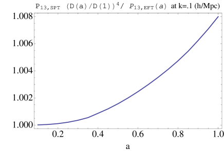
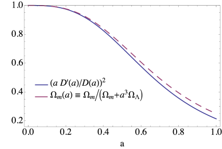
Refer to caption
Refer to caption
Figure 7: We plot the ratio as a function of time of P13subscript𝑃13P_{13} and P22subscript𝑃22P_{22} as obtained using the rigorous time dependence and the approximate one. The ratio goes to 1 at early times when dark energy is irrelevant and the approximate treatment becomes exact. The results at redshift zero agree well, at percent level.
Refer to caption
Refer to caption
Figure 8: Plot of the ratio Ωm(a)/(logD/loga)2subscriptΩ𝑚𝑎superscript𝐷𝑎2\Omega_{m}(a)/({\partial}\log D/{\partial}\log a)^{2}. This being equal to one would justify the approximations done in this appendix. We see that at late times the difference is quite large. Since this is a correction to the one-loop term, this error can be acceptable for a one-loop calculation. On the contrary the approximation can become more harmful if one goes to higher loops. The actual result on the power spectrum of the approximation is even better than what shown in the plot, as more of the clustering happens before dark energy domination.

Appendix D Measuring in N𝑁N-body simulations

D.1 Efficient calculation

We break the calculation into three parts: the calculation of primary fields, the calculation of secondary fields, and the calculation of correlations. Primary fields are dependent solely upon the positions or velocities of the simulation particles, and secondary fields are dependent upon the primary fields, and we care about correlations between particular secondary fields.

The immediate goal is to calculate the following expressions:

cs2(r)superscriptsubscript𝑐𝑠2𝑟\displaystyle c_{s}^{2}(r) =PAΘ2PδΘPAδ2PΘΘ(2PδΘ)22Pδδ2PΘΘabsentsubscript𝑃𝐴Θsuperscript2subscript𝑃𝛿Θsubscript𝑃𝐴𝛿superscript2subscript𝑃ΘΘsuperscriptsuperscript2subscript𝑃𝛿Θ2superscript2subscript𝑃𝛿𝛿superscript2subscript𝑃ΘΘ\displaystyle=\frac{P_{A\Theta}\partial^{2}P_{\delta\Theta}-P_{A\delta}\partial^{2}P_{\Theta\Theta}}{(\partial^{2}P_{\delta\Theta})^{2}-\partial^{2}P_{\delta\delta}\partial^{2}P_{\Theta\Theta}} (85)
cv2(r)superscriptsubscript𝑐𝑣2𝑟\displaystyle c_{v}^{2}(r) =PAδ2PδΘPAΘ2Pδδ(2PδΘ)22Pδδ2PΘΘabsentsubscript𝑃𝐴𝛿superscript2subscript𝑃𝛿Θsubscript𝑃𝐴Θsuperscript2subscript𝑃𝛿𝛿superscriptsuperscript2subscript𝑃𝛿Θ2superscript2subscript𝑃𝛿𝛿superscript2subscript𝑃ΘΘ\displaystyle=\frac{P_{A\delta}\partial^{2}P_{\delta\Theta}-P_{A\Theta}\partial^{2}P_{\delta\delta}}{(\partial^{2}P_{\delta\Theta})^{2}-\partial^{2}P_{\delta\delta}\partial^{2}P_{\Theta\Theta}} (86)

based upon the two-point correlation functions: PIJ(r)subscript𝑃𝐼𝐽𝑟P_{IJ}(r). These two point correlation functions can be seen as the expectation value of the product of field I𝐼I with field J𝐽J, but with I𝐼I evaluated at all points a distance r𝑟r from all points rsuperscript𝑟r^{\prime}:

PIJ(r)I(r+r)J(r)Ω(r,r),r=limR316π2R30R𝑑r𝑑Ω𝑑Ωr2I(r+r)J(r).subscript𝑃𝐼𝐽𝑟subscriptdelimited-⟨⟩𝐼𝑟superscript𝑟𝐽superscript𝑟Ωsuperscript𝑟𝑟superscript𝑟subscript𝑅316superscript𝜋2superscript𝑅3superscriptsubscript0𝑅differential-dsuperscript𝑟differential-dsuperscriptΩdifferential-dΩsuperscript𝑟2𝐼𝑟superscript𝑟𝐽superscript𝑟P_{IJ}(r)\equiv\langle I(\vec{r}+\vec{r}\,^{\prime})J(\vec{r}\,^{\prime})\rangle_{\Omega(r^{\prime},r),r^{\prime}}=\lim_{R\rightarrow\infty}\frac{3}{16\pi^{2}R^{3}}\int_{0}^{R}\,dr^{\prime}\,d\Omega^{\prime}\,d\Omega\,r^{\prime 2}\,I(\vec{r}+\vec{r}\,^{\prime})\,J(\vec{r}\,^{\prime}). (87)

In the quantities being calculated the overall normalization cancels. The cost of evaluating each of these fields at all positions is prohibitive, so we approximate these correlations by measuring some large N𝑁N number of pairs of points (pseudo)-randomly chosen but at fixed r𝑟r:

P^IJ(r)N1{ra,rb}Nset(r)I(ra)J(rb)subscript^𝑃𝐼𝐽𝑟superscript𝑁1subscriptsuperscriptsubscript𝑟𝑎superscriptsubscript𝑟𝑏subscript𝑁set𝑟𝐼superscriptsubscript𝑟𝑎𝐽superscriptsubscript𝑟𝑏\hat{P}_{IJ}(r)\approx N^{-1}\!\!\!\!\!\!\!\!\sum_{\{\vec{r}_{a}\,^{\prime},\vec{r}_{b}\,^{\prime}\}\in N_{\rm set}(r)}\!\!\!\!\!\!\!\!I(\vec{r}_{a}\,^{\prime})~{}J(\vec{r}_{b}\,^{\prime}) (88)

where Nset(r)subscript𝑁set𝑟N_{\rm set}(r) is a set of N𝑁N pairs of points randomly selected from the space to be separated by a distance r𝑟r.

The following are the specific correlation functions used:

PAδ(r)subscript𝑃𝐴𝛿𝑟\displaystyle P_{A\delta}(r) =As(r+r)δl(r)Ω(r,r),rabsentsubscriptdelimited-⟨⟩subscript𝐴𝑠𝑟superscript𝑟subscript𝛿𝑙superscript𝑟Ωsuperscript𝑟𝑟superscript𝑟\displaystyle=\langle A_{s}(\vec{r}+\vec{r}\,^{\prime})\delta_{l}(\vec{r}\,^{\prime})\rangle_{\Omega(r^{\prime},r),r^{\prime}} (89)
PAΘ(r)subscript𝑃𝐴Θ𝑟\displaystyle P_{A\Theta}(r) =As(r+r)Θl(r)Ω(r,r),rabsentsubscriptdelimited-⟨⟩subscript𝐴𝑠𝑟superscript𝑟subscriptΘ𝑙superscript𝑟Ωsuperscript𝑟𝑟superscript𝑟\displaystyle=\langle A_{s}(\vec{r}+\vec{r}\,^{\prime})\Theta_{l}(\vec{r}\,^{\prime})\rangle_{\Omega(r^{\prime},r),r^{\prime}} (90)
Pδδ(r)subscript𝑃𝛿𝛿𝑟\displaystyle P_{\delta\delta}(r) =δl(r+r)δl(r)Ω(r,r),rabsentsubscriptdelimited-⟨⟩subscript𝛿𝑙𝑟superscript𝑟subscript𝛿𝑙superscript𝑟Ωsuperscript𝑟𝑟superscript𝑟\displaystyle=\langle\delta_{l}(\vec{r}+\vec{r}\,^{\prime})\delta_{l}(\vec{r}\,^{\prime})\rangle_{\Omega(r^{\prime},r),r^{\prime}} (91)
PδΘ(r)subscript𝑃𝛿Θ𝑟\displaystyle P_{\delta\Theta}(r) =δl(r+r)Θl(r)Ω(r,r),rabsentsubscriptdelimited-⟨⟩subscript𝛿𝑙𝑟superscript𝑟subscriptΘ𝑙superscript𝑟Ωsuperscript𝑟𝑟superscript𝑟\displaystyle=\langle\delta_{l}(\vec{r}+\vec{r}\,^{\prime})\Theta_{l}(\vec{r}\,^{\prime})\rangle_{\Omega(r^{\prime},r),r^{\prime}} (92)
PΘΘ(r)subscript𝑃ΘΘ𝑟\displaystyle P_{\Theta\Theta}(r) =Θl(r+r)Θl(r)Ω(r,r),rabsentsubscriptdelimited-⟨⟩subscriptΘ𝑙𝑟superscript𝑟subscriptΘ𝑙superscript𝑟Ωsuperscript𝑟𝑟superscript𝑟\displaystyle=\langle\Theta_{l}(\vec{r}+\vec{r}\,^{\prime})\Theta_{l}(\vec{r}\,^{\prime})\rangle_{\Omega(r^{\prime},r),r^{\prime}} (93)
2Pδδ(r)superscript2subscript𝑃𝛿𝛿𝑟\displaystyle\partial^{2}P_{\delta\delta}(r) =2δl(r+r)δl(r)Ω(r,r),rabsentsubscriptdelimited-⟨⟩superscript2subscript𝛿𝑙𝑟superscript𝑟subscript𝛿𝑙superscript𝑟Ωsuperscript𝑟𝑟superscript𝑟\displaystyle=\langle\partial^{2}\delta_{l}(\vec{r}+\vec{r}\,^{\prime})\,\delta_{l}(\vec{r}\,^{\prime})\rangle_{\Omega(r^{\prime},r),r^{\prime}} (94)
2PδΘ(r)superscript2subscript𝑃𝛿Θ𝑟\displaystyle\partial^{2}P_{\delta\Theta}(r) =2δl(r+r)Θl(r)Ω(r,r),rabsentsubscriptdelimited-⟨⟩superscript2subscript𝛿𝑙𝑟superscript𝑟subscriptΘ𝑙superscript𝑟Ωsuperscript𝑟𝑟superscript𝑟\displaystyle=\langle\partial^{2}\delta_{l}(\vec{r}+\vec{r}\,^{\prime})\,\Theta_{l}(\vec{r}\,^{\prime})\rangle_{\Omega(r^{\prime},r),r^{\prime}} (95)
2PΘΘ(r)superscript2subscript𝑃ΘΘ𝑟\displaystyle\partial^{2}P_{\Theta\Theta}(r) =2Θl(r+r)Θl(r)Ω(r,r),rabsentsubscriptdelimited-⟨⟩superscript2subscriptΘ𝑙𝑟superscript𝑟subscriptΘ𝑙superscript𝑟Ωsuperscript𝑟𝑟superscript𝑟\displaystyle=\langle\partial^{2}\Theta_{l}(\vec{r}+\vec{r}\,^{\prime})\,\Theta_{l}(\vec{r}\,^{\prime})\rangle_{\Omega(r^{\prime},r),r^{\prime}} (96)

These are functions of the gravitational short-mode field Assubscript𝐴𝑠A_{s}, the over density δ𝛿\delta, and the velocity divergence ΘΘ\Theta, and relevant spatial derivatives. These fields are to be calculated from the observed (or simulated) positions and velocities of point-sources at a fixed moment in time (redshift=0 initially). We smear the observation of the position of these sources with a gaussian, introducing a (soft) ultraviolet cutoff.

To calculate cs2superscriptsubscript𝑐𝑠2c_{s}^{2} and cv2superscriptsubscript𝑐𝑣2c_{v}^{2} in terms of As,δ,Θ,2δ,2Θsubscript𝐴𝑠𝛿Θsuperscript2𝛿superscript2ΘA_{s},\delta,\Theta,\partial^{2}\delta,\partial^{2}\Theta we use a number of secondary fields. While it would be possible to numerically estimate the relative necessary spatial derivatives, it is simple enough to explicitly carry the operations out analytically, and treat them as independent secondary fields, avoiding the introduction of specious numerical error.

[δ](r)delimited-[]𝛿𝑟\displaystyle[\delta]({\vec{r}}) =[ρ](r)/ρb1,absentdelimited-[]𝜌𝑟subscript𝜌𝑏1\displaystyle=[\rho]({\vec{r}})/\rho_{b}-1\,, (97)
[Θ](r)delimited-[]Θ𝑟\displaystyle[\Theta]({\vec{r}}) =1Hai=13[ivi](r)absent1𝐻𝑎superscriptsubscript𝑖13delimited-[]subscript𝑖subscript𝑣𝑖𝑟\displaystyle=-\frac{1}{Ha}\sum_{i=1}^{3}{[\partial_{i}v_{i}]({\vec{r}})}\, (98)
[As](r)delimited-[]subscript𝐴𝑠𝑟\displaystyle[A_{s}]({\vec{r}}) =1ρbi=13([iiϕs](r)+j=13[ijκij](r)),absent1subscript𝜌𝑏superscriptsubscript𝑖13delimited-[]subscript𝑖subscript𝑖subscriptitalic-ϕ𝑠𝑟superscriptsubscript𝑗13delimited-[]subscript𝑖subscript𝑗subscript𝜅𝑖𝑗𝑟\displaystyle=\frac{1}{\rho_{b}}\sum_{i=1}^{3}{\left([\partial_{i}\partial_{i}\phi_{s}]({\vec{r}})+\sum_{j=1}^{3}[\partial_{i}\partial_{j}\kappa_{ij}]({\vec{r}})\right)}\,, (99)
[2δ](r)delimited-[]superscript2𝛿𝑟\displaystyle[\partial^{2}\delta]({\vec{r}}) =i=13[i2ρ](r)/ρb,absentsuperscriptsubscript𝑖13delimited-[]superscriptsubscript𝑖2𝜌𝑟subscript𝜌𝑏\displaystyle=\sum_{i=1}^{3}[\partial_{i}^{2}\rho]({\vec{r}})/\rho_{b}\,, (100)
[2Θ](r)delimited-[]superscript2Θ𝑟\displaystyle[\partial^{2}\Theta]({\vec{r}}) =1Hai=1,j=13[i2jvj](r)absent1𝐻𝑎superscriptsubscriptformulae-sequence𝑖1𝑗13delimited-[]superscriptsubscript𝑖2subscript𝑗subscript𝑣𝑗𝑟\displaystyle=-\frac{1}{Ha}\sum_{i=1,j=1}^{3}{[\partial_{i}^{2}\partial_{j}v_{j}]({\vec{r}})}\, (101)
[ijϕs](r)delimited-[]subscript𝑖subscript𝑗subscriptitalic-ϕ𝑠𝑟\displaystyle[\partial_{i}\partial_{j}\phi_{s}]({\vec{r}}) =[i[ρmjϕ]Λs)](r)+4πGa22Λ2([iρ](r)[jρ](r)+[ρ](r)[ijρ](r))\displaystyle=[\partial_{i}[\rho_{m}\partial_{j}\phi]_{\Lambda s})]({\vec{r}})+\frac{4\pi Ga^{2}}{2\Lambda^{2}}\left([\partial_{i}\rho]({\vec{r}})[\partial_{j}\rho]({\vec{r}})+[\rho]({\vec{r}})[\partial_{i}\partial_{j}\rho]({\vec{r}})\right) (102)
[ijκij](r)delimited-[]subscript𝑖subscript𝑗subscript𝜅𝑖𝑗𝑟\displaystyle[\partial_{i}\partial_{j}\kappa_{ij}]({\vec{r}}) =[ijσij](r)[jπi](r)[ivj](r)[iπi](r)[jvj](r)absentdelimited-[]subscript𝑖subscript𝑗subscript𝜎𝑖𝑗𝑟delimited-[]subscript𝑗subscript𝜋𝑖𝑟delimited-[]subscript𝑖subscript𝑣𝑗𝑟delimited-[]subscript𝑖subscript𝜋𝑖𝑟delimited-[]subscript𝑗subscript𝑣𝑗𝑟\displaystyle=[\partial_{i}\partial_{j}\sigma_{ij}]({\vec{r}})-[\partial_{j}\pi_{i}]({\vec{r}})\,[\partial_{i}v_{j}]({\vec{r}})-[\partial_{i}\pi_{i}]({\vec{r}})[\partial_{j}v_{j}]({\vec{r}}) (103)
[πi](r)[ijvj](r)[ijπi](r)[vj](r)delimited-[]subscript𝜋𝑖𝑟delimited-[]subscript𝑖subscript𝑗subscript𝑣𝑗𝑟delimited-[]subscript𝑖subscript𝑗subscript𝜋𝑖𝑟delimited-[]subscript𝑣𝑗𝑟\displaystyle~{}-[\pi_{i}]({\vec{r}})\,[\partial_{i}\partial_{j}v_{j}]({\vec{r}})-[\partial_{i}\partial_{j}\pi_{i}]({\vec{r}})\,[v_{j}]({\vec{r}})
[vi](r)delimited-[]subscript𝑣𝑖𝑟\displaystyle[v_{i}]({\vec{r}}) =[πi](r)/[ρ](r)absentdelimited-[]subscript𝜋𝑖𝑟delimited-[]𝜌𝑟\displaystyle=[\pi_{i}]({\vec{r}})/[\rho]({\vec{r}}) (104)
[ivj](r)delimited-[]subscript𝑖subscript𝑣𝑗𝑟\displaystyle[\partial_{i}v_{j}]({\vec{r}}) =[iπj](r)/[ρ](r)[πj](r)[iρ](r)/([ρ](r))2absentdelimited-[]subscript𝑖subscript𝜋𝑗𝑟delimited-[]𝜌𝑟delimited-[]subscript𝜋𝑗𝑟delimited-[]subscript𝑖𝜌𝑟superscriptdelimited-[]𝜌𝑟2\displaystyle=[\partial_{i}\pi_{j}]({\vec{r}})/[\rho]({\vec{r}})-[\pi_{j}]({\vec{r}})[\partial_{i}\rho]({\vec{r}})/([\rho]({\vec{r}}))^{2} (105)
[ijvk](r)delimited-[]subscript𝑖subscript𝑗subscript𝑣𝑘𝑟\displaystyle\ [\partial_{i}\partial_{j}v_{k}]({\vec{r}}) =[ijπk](r)/[ρ](r)[iπk](r)[jρ]/([ρ](r))2[jπk](r)[iρ]/([ρ](r))2absentdelimited-[]subscript𝑖subscript𝑗subscript𝜋𝑘𝑟delimited-[]𝜌𝑟delimited-[]subscript𝑖subscript𝜋𝑘𝑟delimited-[]subscript𝑗𝜌superscriptdelimited-[]𝜌𝑟2delimited-[]subscript𝑗subscript𝜋𝑘𝑟delimited-[]subscript𝑖𝜌superscriptdelimited-[]𝜌𝑟2\displaystyle=[\partial_{i}\partial_{j}\pi_{k}]({\vec{r}})/[\rho]({\vec{r}})-[\partial_{i}\pi_{k}]({\vec{r}})[\partial_{j}\rho]/([\rho]({\vec{r}}))^{2}-[\partial_{j}\pi_{k}]({\vec{r}})[\partial_{i}\rho]/([\rho]({\vec{r}}))^{2} (106)
[πk](r)[ijρ](r)/([ρ](r))2+2[πk](r)[iρ](r)[jρ](r)/([ρ](r))3delimited-[]subscript𝜋𝑘𝑟delimited-[]subscript𝑖subscript𝑗𝜌𝑟superscriptdelimited-[]𝜌𝑟22delimited-[]subscript𝜋𝑘𝑟delimited-[]subscript𝑖𝜌𝑟delimited-[]subscript𝑗𝜌𝑟superscriptdelimited-[]𝜌𝑟3\displaystyle-[\pi_{k}]({\vec{r}})[\partial_{i}\partial_{j}\rho]({\vec{r}})/([\rho]({\vec{r}}))^{2}+2[\pi_{k}]({\vec{r}})[\partial_{i}\rho]({\vec{r}})[\partial_{j}\rho]({\vec{r}})/([\rho]({\vec{r}}))^{3}
[i2jvj](r)delimited-[]superscriptsubscript𝑖2subscript𝑗subscript𝑣𝑗𝑟\displaystyle[\partial_{i}^{2}\partial_{j}v_{j}]({\vec{r}}) =([ρ](r))4{6([iρ](r))2[jρ](r)[πj](r)\displaystyle=([\rho]({\vec{r}}))^{-4}\Big{\{}-6\,([\partial_{i}\rho]({\vec{r}}))^{2}\,[\partial_{j}\rho]({\vec{r}})\,[\pi_{j}]({\vec{r}}) (107)
+2(([iρ](r))2[jπj](r)+[iiρ](r)[jρ](r)[πj](r)\displaystyle~{}+2\,\Big{(}([\partial_{i}\rho]({\vec{r}}))^{2}\,[\partial_{j}\pi_{j}]({\vec{r}})+[\partial_{i}\partial_{i}\rho]({\vec{r}})\,[\partial_{j}\rho]({\vec{r}})\,[\pi_{j}]({\vec{r}})
+2[ρ](r)[iρ](r)([iπj](r)[jρ](r)+[ijρ](r)[πj](r)))\displaystyle~{}+2\,[\rho]({\vec{r}})\,[\partial_{i}\rho]({\vec{r}})\,([\partial_{i}\pi_{j}]({\vec{r}})\,[\partial_{j}\rho]({\vec{r}})+[\partial_{i}\partial_{j}\rho]({\vec{r}})\,[\pi_{j}]({\vec{r}}))\Big{)}
([ρ](r))2(2[ijρ](r)[iπj](r)+2[ijπj](r)([iρ](r))\displaystyle~{}-\,\,([\rho]({\vec{r}}))^{2}\,\Big{(}2\,[\partial_{i}\partial_{j}\rho]({\vec{r}})\,[\partial_{i}\pi_{j}]({\vec{r}})+2\,[\partial_{i}\partial_{j}\pi_{j}]({\vec{r}})\,([\partial_{i}\rho]({\vec{r}}))
+[iiρ](r)[jπj](r)+[iiπj](r)[jρ](r)+[i2jρ](r)[πj](r))\displaystyle~{}+[\partial_{i}\partial_{i}\rho]({\vec{r}})\,[\partial_{j}\pi_{j}]({\vec{r}})+[\partial_{i}\partial_{i}\pi_{j}]({\vec{r}})\,[\partial_{j}\rho]({\vec{r}})+[\partial_{i}^{2}\partial_{j}\rho]({\vec{r}})\,[\pi_{j}]({\vec{r}})\Big{)}
+([ρ](r))3[iijπj](r)}\displaystyle~{}+([\rho]({\vec{r}}))^{3}\,[\partial_{i}\partial_{i}\partial_{j}\pi_{j}]({\vec{r}})\Big{\}}

These are, in turn, defined in terms of the following primary fields

[ρ](r)delimited-[]𝜌𝑟\displaystyle\left[\rho\right]({\vec{r}}) =mΛ3/(a3(2π)3/2)nη(r)W(rrn)absent𝑚superscriptΛ3superscript𝑎3superscript2𝜋32subscript𝑛𝜂𝑟𝑊𝑟subscript𝑟𝑛\displaystyle=m\Lambda^{3}/(a^{3}(2\pi)^{3/2})\sum_{n\in\eta({\vec{r}})}W({\vec{r}}-\vec{r}_{n}) (108)
[iρ](r)delimited-[]subscript𝑖𝜌𝑟\displaystyle\left[\partial_{i}\rho\right]({\vec{r}}) =mΛ3/(a3(2π)3/2)nη(r)iW(rrn)absent𝑚superscriptΛ3superscript𝑎3superscript2𝜋32subscript𝑛𝜂𝑟subscript𝑖𝑊𝑟subscript𝑟𝑛\displaystyle=m\Lambda^{3}/(a^{3}(2\pi)^{3/2})\sum_{n\in\eta({\vec{r}})}\partial_{i}W({\vec{r}}-\vec{r}_{n}) (109)
[ijρ](r)delimited-[]subscript𝑖subscript𝑗𝜌𝑟\displaystyle\left[\partial_{i}\partial_{j}\rho\right]({\vec{r}}) =mΛ3/(a3(2π)3/2)nη(r)ijW(rrn)absent𝑚superscriptΛ3superscript𝑎3superscript2𝜋32subscript𝑛𝜂𝑟subscript𝑖subscript𝑗𝑊𝑟subscript𝑟𝑛\displaystyle=m\Lambda^{3}/(a^{3}(2\pi)^{3/2})\sum_{n\in\eta({\vec{r}})}\partial_{i}\partial_{j}W({\vec{r}}-\vec{r}_{n}) (110)
[(i)2jρ](r)delimited-[]superscriptsubscript𝑖2subscript𝑗𝜌𝑟\displaystyle\left[(\partial_{i})^{2}\partial_{j}\rho\right]({\vec{r}}) =mΛ3/(a3(2π)3/2)nη(r)(i)2jW(rrn)absent𝑚superscriptΛ3superscript𝑎3superscript2𝜋32subscript𝑛𝜂𝑟superscriptsubscript𝑖2subscript𝑗𝑊𝑟subscript𝑟𝑛\displaystyle=m\Lambda^{3}/(a^{3}(2\pi)^{3/2})\sum_{n\in\eta({\vec{r}})}(\partial_{i})^{2}\partial_{j}W({\vec{r}}-\vec{r}_{n}) (111)
[πi](r)delimited-[]subscript𝜋𝑖𝑟\displaystyle\left[\pi_{i}\right]({\vec{r}}) =mΛ3/(a3(2π)3/2)nη(r)W(rrn)(vn)iabsent𝑚superscriptΛ3superscript𝑎3superscript2𝜋32subscript𝑛𝜂𝑟𝑊𝑟subscript𝑟𝑛subscriptsubscript𝑣𝑛𝑖\displaystyle=m\Lambda^{3}/(a^{3}(2\pi)^{3/2})\sum_{n\in\eta({\vec{r}})}W({\vec{r}}-\vec{r}_{n})(\vec{v}_{n})_{i} (112)
[iπj](r)delimited-[]subscript𝑖subscript𝜋𝑗𝑟\displaystyle\left[\partial_{i}\pi_{j}\right]({\vec{r}}) =mΛ3/(a3(2π)3/2)nη(r)iW(rrn)(vn)jabsent𝑚superscriptΛ3superscript𝑎3superscript2𝜋32subscript𝑛𝜂𝑟subscript𝑖𝑊𝑟subscript𝑟𝑛subscriptsubscript𝑣𝑛𝑗\displaystyle=m\Lambda^{3}/(a^{3}(2\pi)^{3/2})\sum_{n\in\eta({\vec{r}})}\partial_{i}W({\vec{r}}-\vec{r}_{n})(\vec{v}_{n})_{j} (113)
[ijπk](r)delimited-[]subscript𝑖subscript𝑗subscript𝜋𝑘𝑟\displaystyle\left[\partial_{i}\partial_{j}\pi_{k}\right]({\vec{r}}) =mΛ3/(a3(2π)3/2)nη(r)ijW(rrn)(vn)kabsent𝑚superscriptΛ3superscript𝑎3superscript2𝜋32subscript𝑛𝜂𝑟subscript𝑖subscript𝑗𝑊𝑟subscript𝑟𝑛subscriptsubscript𝑣𝑛𝑘\displaystyle=m\Lambda^{3}/(a^{3}(2\pi)^{3/2})\sum_{n\in\eta({\vec{r}})}\partial_{i}\partial_{j}W({\vec{r}}-\vec{r}_{n})(\vec{v}_{n})_{k} (114)
[(i)2jπk](r)delimited-[]superscriptsubscript𝑖2subscript𝑗subscript𝜋𝑘𝑟\displaystyle\left[(\partial_{i})^{2}\partial_{j}\pi_{k}\right]({\vec{r}}) =mΛ3/(a3(2π)3/2)nη(r)(i)2jW(rrn)(vn)kabsent𝑚superscriptΛ3superscript𝑎3superscript2𝜋32subscript𝑛𝜂𝑟superscriptsubscript𝑖2subscript𝑗𝑊𝑟subscript𝑟𝑛subscriptsubscript𝑣𝑛𝑘\displaystyle=m\Lambda^{3}/(a^{3}(2\pi)^{3/2})\sum_{n\in\eta({\vec{r}})}(\partial_{i})^{2}\partial_{j}W({\vec{r}}-\vec{r}_{n})(\vec{v}_{n})_{k} (115)
[ijσij](r)delimited-[]subscript𝑖subscript𝑗subscript𝜎𝑖𝑗𝑟\displaystyle\left[\partial_{i}\partial_{j}\sigma_{ij}\right]({\vec{r}}) =mΛ3/(a3(2π)3/2)nη(r)ijW(rrn)(vn)i(vn)jabsent𝑚superscriptΛ3superscript𝑎3superscript2𝜋32subscript𝑛𝜂𝑟subscript𝑖subscript𝑗𝑊𝑟subscript𝑟𝑛subscriptsubscript𝑣𝑛𝑖subscriptsubscript𝑣𝑛𝑗\displaystyle=m\Lambda^{3}/(a^{3}(2\pi)^{3/2})\sum_{n\in\eta({\vec{r}})}\partial_{i}\partial_{j}W({\vec{r}}-\vec{r}_{n})(\vec{v}_{n})_{i}(\vec{v}_{n})_{j} (116)
[i[ρmjϕ]Λs](r)delimited-[]subscript𝑖subscriptdelimited-[]subscript𝜌𝑚subscript𝑗italic-ϕΛ𝑠𝑟\displaystyle\left[\partial_{i}[\rho_{m}\partial_{j}\phi]_{\Lambda s}\right]({\vec{r}}) =m2G/a4(Λ/2π)3nη(r)(iW(rrn))(ξn)jabsentsuperscript𝑚2𝐺superscript𝑎4superscriptΛ2𝜋3subscript𝑛𝜂𝑟subscript𝑖𝑊𝑟subscript𝑟𝑛subscriptsubscript𝜉𝑛𝑗\displaystyle=m^{2}G/a^{4}(\Lambda/\sqrt{2\pi})^{3}\sum_{n\in\eta({\vec{r}})}(\partial_{i}W({{\vec{r}}-\vec{r}_{n}}))(\xi_{n})_{j} (117)

where μrmax𝜇subscript𝑟max\mu\equiv r_{\rm max} and η(r)={ns.t.|rrn|<rmax}\eta({\vec{r}})=\{n~{}{\rm s.t.}~{}\left|{{\vec{r}}-\vec{r}_{n}}\right|<r_{\rm max}\}, and we have introduced the following functions for notational convenience:

W(r)𝑊𝑟\displaystyle W(r) exp(Λ22r2)absentsuperscriptΛ22superscript𝑟2\displaystyle\equiv\exp\left(-\frac{\Lambda^{2}}{2}r^{2}\right) (118)
iW(r)subscript𝑖𝑊𝑟\displaystyle\ \partial_{i}W(r) Λ2riW(r)absentsuperscriptΛ2subscript𝑟𝑖𝑊𝑟\displaystyle\equiv-\Lambda^{2}r_{i}W(r) (119)
ijW(r)subscript𝑖subscript𝑗𝑊𝑟\displaystyle\partial_{i}\partial_{j}W(r) Λ2W(r)(Λ2rirjδkij)absentsuperscriptΛ2𝑊𝑟superscriptΛ2subscript𝑟𝑖subscript𝑟𝑗subscriptsuperscript𝛿𝑖𝑗k\displaystyle\equiv\Lambda^{2}W(r)(\Lambda^{2}r_{i}r_{j}-\delta^{ij}_{\rm k}) (120)
(i)2jW(r)superscriptsubscript𝑖2subscript𝑗𝑊𝑟\displaystyle(\partial_{i})^{2}\partial_{j}W(r) Λ2(iW(r)(Λ2rirjδkij)+W(r)Λ2(𝟏irj+δkijri)))\displaystyle\equiv\Lambda^{2}\left(\partial_{i}W(r)\left(\Lambda^{2}r_{i}r_{j}-\delta^{ij}_{\rm k}\right)+W(r)\Lambda^{2}({\mathbf{1}}_{i}\,r_{j}+\delta^{ij}_{\rm k}r_{i}))\right) (121)
(ξn)jsubscriptsubscript𝜉𝑛𝑗\displaystyle(\xi_{n})_{j} mηn(rnrm)jΓ(rnrm)(1|rnrm|erfc(Λ|rnrm|/2)\displaystyle\equiv\sum_{m\in\eta_{n}}(\vec{r}_{n}-\vec{r}_{m})_{j}\,\Gamma(\vec{r}_{n}-\vec{r}_{m})\,\Bigg{(}\frac{1}{|\vec{r}_{n}-\vec{r}_{m}|}{\rm erfc}(\Lambda|\vec{r}_{n}-\vec{r}_{m}|/\sqrt{2})
+2πΛW(rnrm)),\displaystyle~{}~{}~{}~{}+\sqrt{\frac{2}{\pi}}\,\Lambda\,W(\vec{r}_{n}-\vec{r}_{m})\Bigg{)}\,, (122)

where ηn={ms.t.|rmrn|<rmax}\eta_{n}=\{m~{}{\rm s.t.}~{}|r_{m}-r_{n}|<r_{\rm max}\}. We set rmax7Λsubscript𝑟max7Λr_{\rm max}\equiv 7\Lambda. It is efficient to precalculate and store (ξn)jsubscriptsubscript𝜉𝑛𝑗(\xi_{n})_{j} for a given downsample of particles and ΛΛ\Lambda. Given that each simulation particle has a limited radius of influence rmaxsubscript𝑟maxr_{\rm max}, a variety of parallelization strategies are available. We have presented these fields, in detail, to emphasize that all such secondary fields rely on a relatively small number of primary fields, and it is only the primary fields which need concern themselves with the explicit number of particles down sampled from the simulation.

D.2 Stability of Measurement and Region Selection

The fluid parameter of interest ccomb2subscriptsuperscript𝑐2comb{c^{2}_{\rm comb}} is calculated as a ratio of polynomial functions of correlations. In fig. 9 we plot the numerator and denominator of these ratios for Λ=1/3(h/Mpc)Λ13𝑀𝑝𝑐\Lambda=1/3\,(h/Mpc) and Λ=1/6(h/Mpc)Λ16𝑀𝑝𝑐\Lambda=1/6\,(h/Mpc). It is worth noting strong confirmation of the effective field theory description is how well the numerator and denominator of the ccomb2subscriptsuperscript𝑐2comb{c^{2}_{\rm comb}} ratio tracks each other. With these sorts of statistical measurements, one should be careful of small fluctuations causing misleading signal near zero over zero regions. For the measurements described in the paper we select a region where the denominator is 3σ3𝜎3\sigma above zero.

Refer to caption
Refer to caption
Figure 9: The numerator and denominators of ccomb2subscriptsuperscript𝑐2comb{c^{2}_{\rm comb}} as measured with smoothing parameter Λ=1/3Λ13\Lambda=1/3 (left) and Λ=1/6Λ16\Lambda=1/6 (right), scaled to similar heights. This allows us to choose a convenient region of measurement to avoid zero over zero contamination. Precision calculations in the future should extend measurements farther into the IR.

Appendix E Renormalizing at finite ΛΛ\Lambda

The procedure as outlined in the main text involves renormalization for Λ=Λ\Lambda=\infty at some chosen krensubscript𝑘renk_{\rm ren} by fitting Pδδ1loopsuperscriptsubscript𝑃𝛿𝛿1loopP_{\delta\delta}^{\rm 1-loop} for ccomb2(Λ)subscriptsuperscript𝑐2combΛ{c^{2}_{\rm comb}}(\Lambda) against observation at that particular krensubscript𝑘renk_{\rm ren}. The power spectrum at all other k𝑘k become predictions of the EFT. We could imagine to perform the same procedure at finite ΛΛ\Lambda. In this case, however, higher derivative terms suppressed by powers of k/Λ𝑘Λk/\Lambda should be included. These terms do indeed vanish as ΛΛ\Lambda\to\infty, but at finite ΛΛ\Lambda and k𝑘k they are not negligible. In fact, as shown in Fig. 10, without the addition of higher derivative terms, the power spectrum deviates from the Λ=Λ\Lambda=\infty as kΛ𝑘Λk\to\Lambda. One can indeed check that the values of ccomb2subscriptsuperscript𝑐2combc^{2}_{\rm comb} that is obtained by fitting in this way is off with respect to the correct value as obtained from running down to finite ΛΛ\Lambda the value of ccomb2subscriptsuperscript𝑐2combc^{2}_{\rm comb} at Λ=Λ\Lambda=\infty by about 15%, depending on the cutoff used, see Fig. 11. Instead, by allowing for higher derivative terms, the correct value of ccomb2subscriptsuperscript𝑐2combc^{2}_{\rm comb} is derived.

Refer to caption
Figure 10: Prediction of the non-linear power spectrum without the addition of higher derivative terms, as we send ΛΛ\Lambda\to\infty, normalized to the non-linear power spectrum. We see that if we keep ΛΛ\Lambda finite, non-included higher derivative terms that scale as powers of k/Λ𝑘Λk/\Lambda are important. Indeed the results improves as Λ=Λ\Lambda=\infty, which is the correct procedure.
Refer to caption
Figure 11: Ratio of the value of ccomb2(Λ,kren)superscriptsubscript𝑐comb2Λsubscript𝑘renc_{\rm comb}^{2}(\Lambda,k_{\rm ren}) as obtained from running from ccomb2(Λ=,kren)superscriptsubscript𝑐comb2Λsubscript𝑘renc_{\rm comb}^{2}(\Lambda=\infty,k_{\rm ren}) versus the one obtained by fitting directly the result of the EFT at finite ΛΛ\Lambda without the inclusion of higher derivative terms in k/Λ𝑘Λk/\Lambda. At low krensubscript𝑘renk_{\rm ren}, the error is particularly pronounced for Λ=1/6Λ16\Lambda=1/6, as in that case kren/Λsubscript𝑘renΛk_{\rm ren}/\Lambda is not very small. Inclusion of higher derivative terms reduces the mismatch to few percent.

References

  • [1] C. Cheung, P. Creminelli, A. L. Fitzpatrick, J. Kaplan and L. Senatore, “The Effective Field Theory of Inflation,” JHEP 0803 (2008) 014 [arXiv:0709.0293 [hep-th]]. L. Senatore and M. Zaldarriaga, “The Effective Field Theory of Multifield Inflation,” JHEP 1204 (2012) 024 [arXiv:1009.2093 [hep-th]].
  • [2] S. Weinberg, “The quantum theory of fields. Vol. 2: Modern applications,” Cambridge, UK: Univ. Pr. (1996) 489 p
  • [3] T. Baldauf, U. Seljak, L. Senatore and M. Zaldarriaga, “Galaxy Bias and non-Linear Structure Formation in General Relativity,” JCAP 1110 (2011) 031 [arXiv:1106.5507 [astro-ph.CO]].
  • [4] D. Baumann, A. Nicolis, L. Senatore and M. Zaldarriaga, “Cosmological Non-Linearities as an Effective Fluid,” arXiv:1004.2488 [astro-ph.CO].
  • [5] F. Bernardeau, S. Colombi, E. Gaztanaga and R. Scoccimarro, “Large scale structure of the universe and cosmological perturbation theory,” Phys. Rept.  367, 1 (2002) [arXiv:astro-ph/0112551].
  • [6] B. Jain and E. Bertschinger, “Second order power spectrum and nonlinear evolution at high redshift,” Astrophys. J.  431, 495 (1994) [arXiv:astro-ph/9311070].
  • [7] M. Shoji, E. Komatsu, “Third-order Perturbation Theory With Non-linear Pressure,” Astrophys. J.  700, 705-719 (2009). [arXiv:0903.2669 [astro-ph.CO]].
  • [8] D. Jeong and E. Komatsu, “Perturbation theory reloaded: analytical calculation of non-linearity in baryonic oscillations in the real space matter power spectrum,” Astrophys. J.  651, 619 (2006) [arXiv:astro-ph/0604075].
  • [9] M. Crocce and R. Scoccimarro, “Renormalized cosmological perturbation theory,” Phys. Rev.  D 73, 063519 (2006) [arXiv:astro-ph/0509418].
  • [10] M. Crocce and R. Scoccimarro, “Nonlinear Evolution of Baryon Acoustic Oscillations,” Phys. Rev.  D 77, 023533 (2008) [arXiv:0704.2783 [astro-ph]].
  • [11] T. Matsubara, “Resumming Cosmological Perturbations via the Lagrangian Picture: One-loop Results in Real Space and in Redshift Space,” Phys. Rev.  D 77 (2008) 063530 [arXiv:0711.2521 [astro-ph]].
  • [12] P. McDonald, “Dark matter clustering: a simple renormalization group approach,” Phys. Rev.  D 75, 043514 (2007) [arXiv:astro-ph/0606028].
  • [13] A. Taruya and T. Hiramatsu, “A Closure Theory for Non-linear Evolution of Cosmological Power Spectra,” arXiv:0708.1367 [astro-ph].
  • [14] K. Izumi and J. Soda, “Renormalized Newtonian Cosmic Evolution with Primordial Non-Gaussanity,” Phys. Rev.  D 76, 083517 (2007) [arXiv:0706.1604 [astro-ph]].
  • [15] S. Matarrese and M. Pietroni, “Baryonic Acoustic Oscillations via the Renormalization Group,” Mod. Phys. Lett.  A 23, 25 (2008) [arXiv:astro-ph/0702653].
  • [16] S. Matarrese and M. Pietroni, “Resumming Cosmic Perturbations,” JCAP 0706, 026 (2007) [arXiv:astro-ph/0703563].
  • [17] T. Nishimichi et al., “Characteristic Scales of Baryon Acoustic Oscillations from Perturbation Theory: Non-linearity and Redshift-Space Distortion Effects,” arXiv:0705.1589 [astro-ph].
  • [18] R. Takahashi, “Third Order Density Perturbation and One-loop Power Spectrum in a Dark Energy Dominated Universe,” Prog. Theor. Phys.  120, 549 (2008) [arXiv:0806.1437 [astro-ph]].
  • [19] J. Carlson, M. White and N. Padmanabhan, “A critical look at cosmological perturbation theory techniques,” Phys. Rev. D 80 (2009) 043531 [arXiv:0905.0479 [astro-ph.CO]].
  • [20] A. L. Fitzpatrick, L. Senatore and M. Zaldarriaga, “Contributions to the Dark Matter 3-Pt Function from the Radiation Era,” JCAP 1005 (2010) 004 [arXiv:0902.2814 [astro-ph.CO]].
  • [21] K. Enqvist and G. Rigopoulos, “Non-linear mode coupling and the growth of perturbations in LCDM,” JCAP 1103 (2011) 005 [arXiv:1008.2751 [astro-ph.CO]].
  • [22] M. Pietroni, G. Mangano, N. Saviano and M. Viel, “Coarse-Grained Cosmological Perturbation Theory,” JCAP 1201 (2012) 019 [arXiv:1108.5203 [astro-ph.CO]].
  • [23] S. Tassev and M. Zaldarriaga, “The Mildly Non-Linear Regime of Structure Formation,” JCAP 1204 (2012) 013 [arXiv:1109.4939 [astro-ph.CO]].
  • [24] S. Tassev and M. Zaldarriaga, “Estimating CDM Particle Trajectories in the Mildly Non-Linear Regime of Structure Formation. Implications for the Density Field in Real and Redshift Space,” arXiv:1203.5785 [astro-ph.CO].
  • [25] S. Tassev and M. Zaldarriaga, “Towards an Optimal Reconstruction of Baryon Oscillations,” arXiv:1203.6066 [astro-ph.CO].
  • [26] L. Senatore and M. Zaldarriaga, “On Loops in Inflation,” JHEP 1012 (2010) 008 [arXiv:0912.2734 [hep-th]].
    L. Senatore and M. Zaldarriaga, “On Loops in Inflation II: IR Effects in Single Clock Inflation,” arXiv:1203.6354 [hep-th].
    G. L. Pimentel, L. Senatore and M. Zaldarriaga, “On Loops in Inflation III: Time Independence of zeta in Single Clock Inflation,” arXiv:1203.6651 [hep-th].
  • [27] J. J. Carrasco, S. Foreman, L. Senatore “1.5 Loops in the Effective Field Theory for Large Scale Structures,” in progress.
  • [28] McBride et al. 2012, in prep.
    P. S. Behroozi, R. H. Wechsler, H. -Y. Wu, M. T. Busha, A. A. Klypin and J. R. Primack, “Gravitationally Consistent Halo Catalogs and Merger Trees for Precision Cosmology,” arXiv:1110.4370 [astro-ph.CO]. http://lss.phy.vanderbilt.edu/lasdamas/simulations.html
  • [29] H. Martel and W. Freudling “Second-order perturbation theory in Omega is not equal to Friedmann models,” Astrophys. J.  371 (1991) 1
  • [30] F. Bernardeau, “Skewness and Kurtosis in large scale cosmic fields,” Astrophys. J.  433 (1994) 1 [astro-ph/9312026].
  • [31] R. Scoccimarro, S. Colombi, J. N. Fry, J. A. Frieman, E. Hivon and A. Melott, “Nonlinear evolution of the bispectrum of cosmological perturbations,” Astrophys. J.  496 (1998) 586 [astro-ph/9704075].