CLaSPS: a new methodology for knowledge extraction from complex astronomical datasets

Abstract

In this paper we present the Clustering-Labels-Score Patterns Spotter (CLaSPS), a new methodology for the determination of correlations among astronomical observables in complex datasets, based on the application of distinct unsupervised clustering techniques. The novelty in CLaSPS is the criterion used for the selection of the optimal clusterings, based on a quantitative measure of the degree of correlation between the cluster memberships and the distribution of a set of observables, the labels, not employed for the clustering. CLaSPS has been primarily developed as a tool to tackle the challenging complexity of the multi-wavelength complex and massive astronomical datasets produced by the federation of the data from modern automated astronomical facilities. In this paper we discuss the applications of CLaSPS to two simple astronomical datasets, both composed of extragalactic sources with photometric observations at different wavelengths from large area surveys. The first dataset, CSC+, is composed of optical quasars spectroscopically selected in the SDSS data, observed in the X-rays by Chandra and with multi-wavelength observations in the near-infrared, optical and ultraviolet spectral intervals. One of the results of the application of CLaSPS to the CSC+ is the re-identification of a well-known correlation between the $\alpha_{\mathrm{OX}}$ parameter and the near ultraviolet color, in a subset of CSC+ sources with relatively small values of the near-ultraviolet colors. The other dataset consists of a sample of blazars for which photometric observations in the optical, mid and near infrared are available, complemented for a subset of the sources, by Fermi $\gamma$-ray data. The main results of the application of CLaSPS to such datasets have been the discovery of a strong correlation between the multi-wavelength color distribution of blazars and their optical spectral classification in BL Lacs and Flat Spectrum Radio Quasars (FSRQs) and a peculiar pattern followed by blazars in the WISE mid-infrared colors space. This pattern and its physical interpretation have been discussed in details in other papers by one of the authors.

1. Introduction

The advancement of discovery in astronomy, from the statistical point of view, can be described as the successful application of several distinct Knowledge Discovery (KD) techniques to increasingly larger data samples. These techniques include: the classification of sources according to one or more observational quantities; pattern recognition for the discovery of correlations among observable quantities; outlier selection for highlighting rare and/or unknown sources; regression, for the estimation of derived empirical properties from observed quantities. The discovery of new or unexpected correlations between observable quantities at different wavelengths, for example, has propelled the understanding of the nature of astronomical sources and their physical modeling (see, for example, the discovery of the fundamental plane of elliptical galaxies (Djorgovski & Davis, 1987)), and the discovery of the link of the galaxy X-ray emission with different stellar populations (Fabbiano & Trinchieri, 1985; Fabbiano & Shapley, 2002).

The effectiveness of pattern recognition techniques for the determination of correlations in low dimensional spaces (two or three dimensions) has usually relied on the ability of the astronomers to visualize the distribution of data and make informed guesses about the nature of these patterns, based on theoretical models, reasonableness and intuition. However, this approach becomes more and more ineffectual with the increase in complexity and size of the explored datasets. This difficulty has led to the introduction of KD techniques in the astronomical context. Such techniques are based on statistical and computational methodologies capable of automatically identifying useful correlations among parameters in a N-dimensional dataset without any a priori assumption on the nature of both data and the sought out patterns. Using these techniques, the focus of the astronomer can shift to the definition of the general problem to be investigated, the selection of the interesting patterns and their physical interpretation. In this paper, we present CLaSPS, a new methodology based on KD techniques for the exploration of complex and massive astronomical datasets and the detection of correlations among observational parameters. While CLaSPS is designed for datasets containing very large number of sources, it is also well suited to handle small datasets, as will be shown in this paper.

The adoption of KD methodologies in astronomy has only recently surged, due to the increasing availability of massive and complex datasets that would be almost intractable if tackled with the knowledge extractions techniques classically employed in astronomical research. A review of the advantages and most interesting applications of KD to astronomical problems can be found in (Ball & Brunner, 2010). The main reasons for the delay in the adoption of such methods in astronomy are: a) datasets for which KD has an edge over classical methods (because of their size and complexity) have become frequent only in the last $\!\sim$15 years; b) slow transition from model-driven to data-driven research; c) lack of interdisciplinary expertise required for the application of KD techniques. Other disciplines for which the problem of dealing with massive datasets arose earlier, instead, have seen a steadier and faster growth of the number and importance of the KD tools employed on a regular basis. For example, the study of financial markets and complex networks and systems (applied to the WWW, advertisement placement, epidemiology, genetics, proteomics and security) have been on the forefront of application and development of KD techniques. Thorough reviews of the applications of KD methodologies to specific financial topics, i.e. customer management and financial fraud detection, can be found in (Ngai et al., 2009) and (Ngai et al., 2011) respectively, while a general review of the role of KD in bio-informatics is provided in (Natarajan et al., 2005). Even if a certain degree of inter-disciplinary expertise is desired, domain-specific knowhow is crucial to narrow down the types and number of techniques that can be used to address the specific problems encountered in each field, and to interpret correctly the results of the application of such techniques to the data. Furthermore, KD is only one of the skills necessary to tackle the new problems arising with the onset of data-driven astronomy, the other being astrostatistics (e.g. Babu & Feigelson, 2007), visualization techniques (Comparato et al., 2007; Way et al., 2011; Hassan & Fluke, 2011) and advanced signal processing (Scargle, 2003; Protopapas et al., 2006). All these fields are currently the subject of a new discipline: the Astroinformatics (Borne et al., 2011).

In this paper, we have focused our attention on the broad question of how efficiently the physical nature of astronomical sources can be characterized by multi-wavelength photometric data. We have applied CLaSPS to two datasets representing specific cases where such assumption can be tested and verified. CLaSPS assumes that low dimensional patterns in data are associated with aggregations (clusters) in the structure of the data in the high-dimensional “feature space” generated by all the observables of the source. These clusters are defined by the degree of correlation between the distribution of features (i.e., the observables used to build the feature space where clusters have been selected) and a set of external quantities, usually observables, metadata or a priori constraints that have not been used for clustering.

The CLaSPS method, based on the KD techniques for unsupervised clustering and the use of external information to label the clusters members, has been designed to tackle the problem of the extraction of information from two distinct classes of datasets: a) inhomogeneous large area datasets. The advancements in the Virtual Observatory (VO) technology are facilitating the access to datasets obtained by the combination of multiple observations from different surveys with different observational features (e.g., depth, spatial coverage and resolution, spectral resolution). Such datasets are, by construction, inherently incomplete and are affected by the inconsistency of the observational features of each set of observations used to create them. We expect these datasets to grow in complexity as new data becomes available. KD techniques can facilitate the extraction of the available knowledge contained in these “federated” inhomogeneous samples. b) Large homogeneous datasets from multi-wavelength surveys of well-defined areas of the sky observed with similar depths at different wavelengths. These surveys typically yield large samples of sources, complete to a given flux. These datasets span limited but well characterized regions of the N-dimensional observable feature space. The exploration of the structure of the multi-dimensional distribution of sources in the feature space may lead to the discovery of high dimensional correlations and patterns in the data that have been overlooked (or, simply, could not be established) in lower dimensional studies.

This paper is organized as follows: in Sec. 2 we describe the CLaSPS method, in Sec. 3 its application to the CSC+ dataset, and in Sec. 4 its application to a sample of blazars with multi-wavelength photometry available. We discuss the future developments of CLaSPS in Sec. 5.

2. CLaSPS

CLaSPS is based on well established data mining techniques for unsupervised clustering. These techniques search for spontaneous and inherent aggregations of data in the feature space generated by their observables. Table LABEL:tab:definitions summarizes the terms that will be used below. These techniques have been complemented by the use of external data (labels). Labels are observables not used for the clustering which can be used to characterize the content of the set of clusters or of single clusters. D’Abrusco et al. (2009) used these techniques for the selection of optical candidate quasars from photometric datasets. They employ as label the spectroscopic classification available for a subset of the photometric sources. This method can be extended to use multiple labels, both numerical (e.g., fluxes, magnitudes, colors) and categorial (spectral classification flags, morphological types). From a methodological standpoint, the two tools required for this KD methodology are:

1. one or more unsupervised clustering algorithms, to determine multiple sets of partitions of the data. (the specific methods used in this paper are discussed in Sec. 2.2);

2. a quantitative measure of the degree of correlation between cluster populations and the values of the label associated with the members of the clusters (see Sec. 2.3 for more details);

Once multiple clusterings of a dataset in a given feature space have been produced, the choice of the most interesting partition of the dataset is performed considering a quantitative evaluation of the degree of correlation between the distribution of the label and the cluster population in each clustering. Unlike most classical criteria selection that rely only on the intrinsic statistical properties of the clusterings, our method selects clusterings based on both the distributions of features and of the associated labels. The degree of correlation between features and labels can be generically expressed by a numerical quantity (the “score”, see Sec. 2.3) that can be defined and calculated for every single clustering and cluster.

Table 1Definitions of the KD-related terms used in the paper.

Term	Definition
Observation	An astronomical source as defined by
	a vector of its observables
Feature	Any observable quantity of a given source
	used to determine a set of clusters
Feature space	An abstract space where each sample is
	represented as points in a N-dimensional space
Cluster	A set of sources (or observations) aggregated
	by a generic clustering algorithm
Clustering	A set of clusters representing a complete
	partition of a sample of observations
Unsupervised	In KD, unsupervised clustering refers to the
clustering	techniques used to determine the spontaneous
	aggregations of sources not using examples
Label	An observable of a set of observations used to
	label the members of the clusters (as defined
	in this paper)
Score	A quantitative diagnostic of the correlation
	between cluster membership and the distribution
	of labels (as defined in this paper)

2.1. CLaSPS and cluster ensembles

The task of combining multiple clusterings into a single partition is known, in the statistical/data mining literature, as the search for the “consensus clustering”. This problem has been thoroughly studied, and is discussed in several papers (e.g. Ghosh & Acharya (2011)). The main reasons for the use of cluster ensembles techniques are: the improvement of the quality of the clustering, increased robustness of the clustering and the ability to combine “multiview” clusterings (i.e. of clusterings obtained with nonidentical sets of sources and/or features) (Ghosh & Acharya, 2011). CLaSPS selects the optimal clustering(s) from the point of view of the astrophysical interpretation of the correlations, according to the values of the scores (Sec. 2.3). The scores are evaluated on the basis the clustering memberships and a given partition the label, an external quantity not used to produce the clusterings. For this reason, CLaSPS neither tries to determine a “consensus clustering” nor attempts to combine clusterings or improve the properties of each distinct clustering produced by the UC methods used. All the clusterings retain their own properties, biases and weaknesses, that have to be taken into account when interpreting the results of the application of CLaSPS. The CLaSPS method could be nonetheless improved by the application of cluster ensembles techniques, as discussed in Sec. 5.

2.2. Unsupervised clustering

In statistical terms, the cluster analysis of a sample is the determination of a segmentation of the data in groups or clusters, each group representing objects with similar properties (Hastie et al., 2009; Hartigan, 1975). The cluster analysis depends on the definition of a “dissimilarity” employed to assign the objects to different clusters. Usually, the dissimilarity is evaluated on general attributes (or features) of the objects. E.g., the values of the observed fluxes in a given filter represent one of the features of an astronomical dataset. The pairwise dissimilarity between the $i$-th and $k$-th observations on the values of the $j$-attribute can be defined as:

$$D(x_{i},x_{k})=\sum_{j=i}^{p}d_{j}(x_{ij},x_{kj})$$ (1)

For quantitative attributes, the pairwise dissimilarity can be evaluated using the squared distance $d_{j}(x_{ij},x_{ik})\!=\!(x_{ij}\!-\!x_{ik})^{2}$. The individual dissimilarities evaluated for each attribute are then combined to produce a single overall dissimilarity between objects. The goal of the clustering algorithm is to partition the sources into clusters so that the pairwise dissimilarities between objects assigned to the same cluster are generally smaller that those in different clusters. In KD the term unsupervised refers to learning algorithm that do not require an example or a “teacher” to infer the properties of the probability density associated with a given dataset (Hastie et al., 2009). The use of unsupervised techniques is relatively new in astronomy, while supervised learning techniques are very common and are usually applied to classification and regression problems. An early example of an application of unsupervised clustering to the problem of the classification of gamma-ray bursts can be found in (Mukherjee et al., 1998). The estimation of photometric redshifts for extragalactic sources, based on the spectroscopic redshifts measured for a subset of the sources has been tackled with several distinct KD methods, for example connectivity analysis (Freeman et al., 2009), gaussian processes (Bonfield et al., 2010; Way & Srivastava, 2006) and neural networks (Yèche et al., 2010; Collister & Lahav, 2004). A further example of the combined use of unsupervised clustering and supervised learning techniques for photometric redshifts estimation can be found in (Laurino et al., 2011). In general, unsupervised learning can be used to highlight the intrinsic structure of the data and as an exploratory tool. For some of these techniques, the only information that has to be provided before the clustering is performed is the final number of clusters. In the following subsections, we will shortly describe the three unsupervised clustering algorithms used in this work.

2.2.1 K-means

The K-means algorithm (Lloyd, 1957) is one of the most frequently used clustering methods. It is applicable when the attributes are quantitative and the dissimilarity measure is defined as the squared euclidean distance: $d(x_{i},x_{k})\!=\!\sum_{j=1}^{p}(x_{ij}\!-\!x_{kj})^{2}\!=\!||x_{ij}\!-\!x_{kj}||^{2}$. The N observations are associated with K clusters so that in a cluster the average dissimilarity of the observations from the cluster mean is minimized. $C^{*}$ is the optimal clustering and $N_{k}$ is the number of observations assigned to the $k$-th cluster, defined as:

$$C^{*}\!=\!\mathrm{min}\!\sum_{k=1}^{K}N_{K}\!\sum_{C(i)=k}\!||x_{i}\!-\!x_{k}||^{2}$$ (2)

2.2.2 Hierarchical clustering

The result of the application of the K-means clustering technique (Sec. 2.2.1) to a dataset depends on $K$, the number of clusters to be searched. Hierarchical clustering methods do not require this number to be specified, instead they do require the user to specify a measure of dissimilarity between groups of observations based on the pairwise dissimilarities among the observations in the two groups. Overall, there are two strategies for hierarchical clustering: agglomerative and divisive.

In the agglomerative strategy, the algorithm starts aggregating at the lowest level possible (each group is composed by only one observation) and at each level (or generation), a pair of clusters is recursively merged into a single cluster. In the divisive strategy, the starting point is the top of the “tree” (all observations in one cluster) and at each level each cluster is recursively split into two new clusters. The merging in the agglomerative method, at each level, involves the aggregation of the two groups with the smallest intergroup dissimilarity. In the divisive methods, instead, at each level the splitting produces two new clusters with the largest possible between-group dissimilarity. Recursive splitting/agglomeration can be represented by a rooted binary tree, where the nodes represent groups. The root node is associated with the whole dataset and each terminal node represents one of the individual observations. A common representation of the hierarchical structure called dendrogram (Hartigan, 1975) is obtained by plotting the binary tree so that the height of each node is proportional to the value of the intergroup dissimilarity between its “children” nodes. Hierarchical clustering techniques impose a hierarchical structure to the data even when such structure does not exists in the data. For this reason, in this paper we will not interpret the clusterings in terms of the properties of the hierarchical structure they belong to, but only in terms of the properties of their feature distribution and of the properties of the distribution of the labels associated with the cluster members.

Agglomerative hierarchical clustering depends on: a) the choice of the definition of pairwise dissimilarity (i.e., dissimilarity between the members of a pair of observations), and b) the agglomeration or “linking” strategy, i.e. the definition of the inter-group dissimilarity, usually based on the pairwise dissimilarity adopted. Several pairwise dissimilarity definitions have been used for the method described in this paper; these include the Euclidean distance (see Eq. (4)), the Manhattan distance (Eq. (5)) (also known as the taxicab distance) and the maximum (or Chebyshev’s) distance (Eq. (6))

$$D(x_{i},x_{k})=\sqrt{\sum_{j=1}^{N}(x_{ij}\!-\!x_{kj})^{2}}$$ (4)

$$D(x_{i},x_{k})=\sum_{j=1}^{N}(\|x_{ij}\!-\!x_{kj}\|)$$ (5)

$$D(x_{i},x_{k})=\mathrm{max}_{i}(\|x_{ij}\!-\!x_{kj}\|)$$ (6)

All the above metrics are suited for continuous measurements associated with the observations. The linking strategies used in this work are described below. The descriptions of the distinct linkage strategies are given in the case of agglomerative clusterings, but they are also valid for divisive clustering methods:

a)

Single linkage: the inter-clusters dissimilarity between two generic clusters $A$ and $B$ can be defined as the minimum pairwise dissimilarity between observations of each cluster:

$$D(A,B)\!=\!\mathrm{min}\{D(x,y):x\in\!A,y\in\!B\}$$ (7)

The clusters are grouped on the basis of the closest couple of members. For this reason, clusters which, on average, are not the closest but which share few nearby observations, can be merged. This is similar to what happens in clustering methods based on the “friends-of-friends” algorithm (Hartigan, 1975);

b)

Complete linkage: the inter-cluster dissimilarity between two clusters $A$ and $B$ can be defined as the maximum pairwise dissimilarity between observations belonging to the two clusters, namely:

$$D(A,B)\!=\!\mathrm{max}\{D(x,y):x\in\!A,y\in\!B\}$$ (8)

In this case, clusters are merged when globally very close to each other, since the condition is on the farthest pair of observations.

c)

Average linkage: the inter-clusters dissimilarity between the two clusters $A$ and $B$ can be defined as the pairwise dissimilarity between the average observations for each clusters:

$$D(A,B)\!=<\!(D(x,y):x\in\!A,y\in\!B)\!>$$ (9)

This case is intermediate between the single linkage and complete linkage strategies. Clusters are merged when they are on average close to each other, i.e. most of observations of each cluster are close to each other. This strategy produces the stablest configuration because it is not sensitive to “outliers”.

d)

Ward’s linkage: the inter-clusters dissimilarity can be defined as a measure of the increase of variance of the cluster obtained by merging the parents clusters compared to the sum of the variances of the two separate clusters:

$$D(A,B)\!=\!\mathrm{ESS}(A,B)-[\mathrm{ESS}(A)\!+\!\mathrm{ESS}(B)]$$ (10)

where:

$$\mathrm{ESS}(A)\!=\!\sum_{i=1}^{N_{A}}\|x_{i}-\frac{1}{N_{A}}\sum_{j=1}^{N_{A}}x_{j}\|^{2}$$ (11)

This linkage strategy provides compact and spherical clusters which, intrinsically, have minimal internal variance (Ward, 1963).

2.2.3 Self Organizing Maps

Self Organizing Maps (SOM) (Kohonen, 1990; Vesanto & Alhoniemi, 2000) are a constrained version of the K-means clustering. In SOM, the “prototypes”, template observations determined on the basis of the initialization of the algorithm, are encouraged to lie on a two-dimensional surface. This manifold is called a constrained topological map, since all the observations in the original feature space are mapped to a two-dimensional coordinate system. A two dimensional grid of prototypes is “bended” by the SOM algorithm to adapt to the observations as accurately as possible. Once reached optimal mapping, the observations can be mapped down onto the “prototypes”, and each observation is assigned to the cluster represented by the closest prototype. Given the $K$ prototypes $m_{k}$ and the $i$-th observation in the p-dimensional feature space $x_{i}$, the closest prototype $m_{j}$ is picked using euclidean distance (4). In the simplest version of the SOM, the position of the prototype is updated according to the rule:

$$m_{k}\leftarrow m_{k}+\alpha(x_{i}-m_{k})$$ (12)

where $\alpha$ is a number called learning rate that changes at each iteration and, usually, goes from $\sim 1$ to 0 over few thousands iterations. The positions of the prototypes are updated until the distance of each observation associated with prototype becomes smaller that a given “distance threshold” $r$. The distance threshold $r$ decreases linearly with each new observation considered, according to the empirical rule followed to update the value of $r$. As in the case of the K-means clustering, the number of prototypes, i.e. of final number of clusters, must be specified by the user. SOM becomes an online version of the K-means algorithm for small $r$ distances, yielding only one observation associated with each prototype. The SOM algorithm can also be used as a supervised classification and regression method, using the stable prototypes definitions obtained using a training, so that “new” sources will be associated with the closest prototype in the feature space. Because of their versatility, SOM have recently been applied to astronomical data to address distinct problems: the selection and classification of extragalactic sources from large surveys data using their photometric attributes (Geach, 2012), the evaluation of photometric redshifts (Geach, 2012; Way & Klose, 2012), spectral classification of stars (Bazarghan, 2012) and the reconstruction of large scale structure of galaxy distribution (Way et al., 2011).

2.3. The Score

As discussed in Sec. 2, the originality of the CLaSPS method lies in the criterion used to select the most meaningful aggregations of sources in the feature space, which is based on the correlation with the labels, i.e. other observables not used to produce the clustering. This correlation is evaluated using a novel indicator, called the score.

Each one of the methods described in the previous paragraphs provides us with one or more clusterings when applied to a given dataset. Each observation is uniquely associated with one of the clusters in the clustering (i.e., each observation belongs to one and only one cluster for each clustering). Additional information available for each source in the dataset, but not used for the clustering (i.e. not used to build the feature space) can be used to label the content of the clusters of each clustering. Categorial labels provide a natural binning; continuous labels, in our method, must be binned for the evaluation of the scores. The binning can be either a set of continuous intervals (for continuous labels) or a set of (single or grouped) values (for categorial labels). The distribution of labels values for the members of each cluster is used to determine the level of correlation between the label and the single cluster. The degrees of correlation between the label distribution and each cluster of a clustering are then combined to provide a measure of the degree of correlation of the label distribution with the clustering as a whole.

The score provides a quantitive measure of the correlation between a label and the cluster membership for a given clustering. For any label $L$ in the set of $N_{L}$ labels available, a binning of $L$ is represented by a set of $M^{(L)}$ classes, either quantitative intervals or categorial values $\{C^{(L)}_{1},C^{(L)}_{2},...,C^{(L)}_{M}\}$. The basic element of the score definition is the fraction $f_{ij}$ of the $i$-th cluster members with values of the label falling in the $j$-th class:

$$f_{ij}=\frac{n_{ij}(L_{i}\in C^{(L)}_{j})}{N_{i}}$$ (13)

where $L_{i}$ is the set of values of the label $L$ associated with the members of the $i$-th cluster, $n_{ij}$ is the number of members of the $i$-th cluster with label values belonging to the $j$-th label class, and $N_{i}$ is the number of members of the $i$-th cluster of the clustering. $F_{ij}=\{F_{i1},F_{i2},...,F_{iM^{(L)}}\}$ can be defined as the arrangement of the fractions $f_{ij}$ sorted in increasing order. The score of the $i$-th cluster of a clustering composed of $N_{\mathrm{clust}}$ clusters relative to the label $L$ can be defined as follows:

$$S_{i}\!=\!\sum_{j=2}^{M^{(L)}}\|F_{ij}\!-\!F_{i(j\!-\!1)}\|$$ (14)

Using the definition of score for a single cluster, the total score of the clustering relative to the label $L$ can be defined as:

$$S_{\mathrm{tot}}\!=\!\frac{1}{N_{\mathrm{clust}}}\!\times\!\sum_{i=1}^{N_{\mathrm{clust}}}S_{i}\!=\!\frac{1}{N_{\mathrm{clust}}}\sum_{i=1}^{N_{\mathrm{clust}}}\!\big{(}\!\sum_{j=2}^{M^{(j)}}\!\|F_{ij}-F_{i(j\!-\!1)}\!\|\big{)}$$ (15)

where $S_{i}$ is the score evaluated for the $i$-th cluster of the clustering defined in (14). By definition, the total score $S_{\mathrm{tot}}$ and each single cluster score $S_{i}$ are normalized to unity.

The weighted total score $S_{\mathrm{tot}}^{{}^{\prime}}$ can be defined as the total normal score $S_{\mathrm{tot}}$ where the score of each cluster is weighted according to the number of sources of the cluster:

$$S_{\mathrm{tot}}^{{}^{\prime}}\!=\!\frac{1}{N_{\mathrm{clust}}}\frac{\sum_{i=1}^{N_{\mathrm{clust}}}N_{i}\!\times\!S_{i}}{\sum_{i=1}^{N_{\mathrm{clust}}}N_{i}}\!=\!\frac{1}{N_{\mathrm{clust}}}\frac{\sum_{i=1}^{N_{\mathrm{clust}}}N_{i}\!\times\!S_{i}}{N_{\mathrm{tot}}}$$ (16)

where $N_{\mathrm{tot}}$ is the total number of sources in the clustering.

The contributions of all clusters to the total $S_{\mathrm{tot}}$ score are equally weighed. For this reason, $S_{\mathrm{tot}}$ is sensitive to small clusters with few members with a large degree of correlation with the label (for example singletons, i.e. clusters composed by only one observation). Instead, the contribution of each cluster to the weighted total score $S_{\mathrm{tot}}^{{}^{\prime}}$ is proportional to the ratio of its members to the total number of observations in the clustering. By definition, $S_{\mathrm{tot}}^{{}^{\prime}}$ is a declining function of the total number of clusters of the clustering. The weighted total score $S_{\mathrm{tot}}^{{}^{\prime}}$ is heavily influenced by the largest clusters and, as a consequence, is a measure of the “mass-weighted” degree of correlation of the dataset. Both $S_{\mathrm{tot}}$ and $S_{\mathrm{tot}}^{{}^{\prime}}$ are used to select the optimal clusterings because they represent complementary measures of distinct aspects of the clusterings, namely the level of correlation of the largest clusters and of the existence of less populated groups of sources.

2.3.1 Score assessment

Before applying the scores to the real astronomical datasets described in Sec. 3 and Sec. 4, we have tested the effectiveness of this method with simulated clusterings. In these simulations, we assume that the final structure of a generic clustering is independent from the unsupervised clustering algorithm used to produce the clustering. This assumption is reasonable because the algorithm depends on the topological relations among the sources of the dataset in the feature space where the clustering has been generated and on the linking strategy used to associate the sources (see Sec. 2.2 for more details). Both the properties of the clustering algorithm and the actual values of the features and labels associated with the simulated sources are of no importance in an idealized description of the clustering, where topological and relational properties of the observations are condensed in the membership, a categorial information, for each source. On these premises, the fundamental parameters describing simulated clusterings are: the total number $N^{\mathrm{(sim)}}_{\mathrm{Tot}}$ of observations of the sample of the simulated clustering; the number of clusters in the clustering $N_{\mathrm{clust}}^{\mathrm{(sim)}}$; the number of members of each cluster, normalized to the total number of observations in the sample $N_{\mathrm{i}}^{\mathrm{(sim)}}$ where $i\in\{1,...,N_{\mathrm{clust}}^{\mathrm{(sim)}}\}$ is associated with the spread of the sizes of the clusters measured with the variance $\sigma^{2}(N_{i}^{(\mathrm{sim})})$; the number of classes of the label $M_{L}^{\mathrm{(sim)}}$; and a prescription to assign the label values to the cluster members.

Three different scenarios have been considered in order to create realistic simulated clusterings. These scenarios have inspired distinct association rules between classes of label values and observations in the clusters that have been used to generate the simulated clusterings. These scenarios are: a) label values belonging to any label class are randomly associated with the observations, regardless of their membership; b) label values of each label class are assigned only to sources belonging to a fixed small number of randomly selected clusters; and c) label values of each label class are assigned to observations in only one randomly selected cluster in the clustering.

We produced simulated clusterings with different degrees of correlation between label values and clusters memberships by mixing the previous three prescriptions in different percentages. Thus, we obtained “recipes” to simulate weak, moderate and strong correlations in clusterings. For the fraction of class label values not randomly associated, each value was assigned only to sources belonging to a randomly picked number of clusters, with one, two or three clusters being the most likely options by definition. The remaining fraction of label values was randomly assigned to sources of the clusterings independently from their cluster memberships.

The weakly correlated clusterings have a 0%-30% not randomly assigned class, the moderately correlated clusterings have 30% to 70% and the extremely correlated clusterings have 70% to 100%. These intervals have been selected in order to verify the effectiveness of the score to express the level of correlation among label distribution and cluster memberships in realistic scenarios where the classes are partially correlated with a subset of clusters, and in the extreme cases with total correlation (100% of not randomly assigned classes) and no correlation (0% of not randomly assigned classes), as a function of the parameters of the simulated clusterings. We produced equal numbers of simulated clusterings for each of the three prescriptions described above. All the parameters of the simulations were free to vary in the intervals described in Table 2, where also the composition of the three classes of clusters is summarized.

Table 2Ranges of the parameters of the simulated clusterings used to validate the effectiveness of the score definitions in capturing the degree of correlation between label value classes and clusters membership distributions

Parameter	Value(s)
$\mathrm{N}^{\mathrm{sim}}$	1000
$\mathrm{N}^{\mathrm{sim}}_{\mathrm{Tot}}$	[30, 200]
$\mathrm{N}^{\mathrm{sim}}_{\mathrm{clust}}$	[3, 12]
$\mathrm{M}^{\mathrm{sim}}_{\mathrm{(L)}}$	[2, 10]
Type of clustering	% not-random/random
Weakly/not corr.	[0%, 30%],[100%, 70%]
Moderately corr.	[30%, 70%],[70%, 30%]
Strongly corr.	[70%, 100%],[30%, 0%]

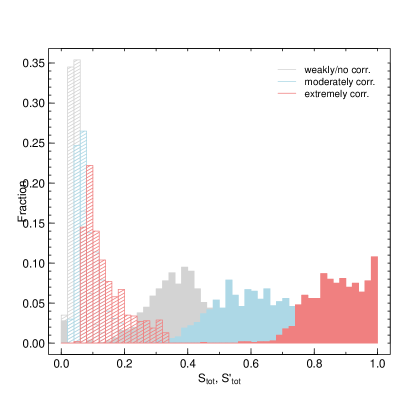
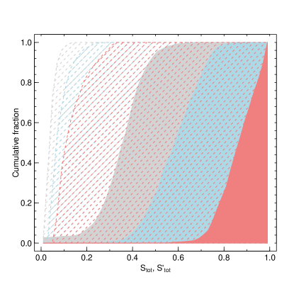
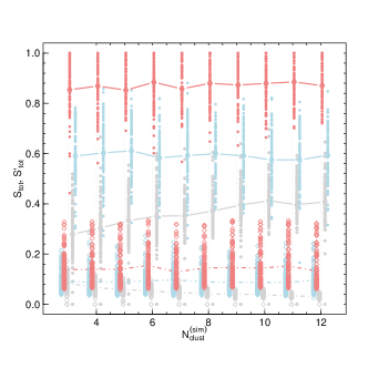
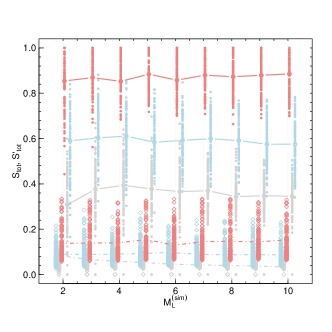
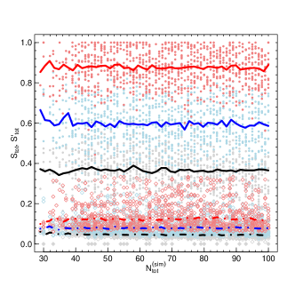
Both normal scores (Eq. (15)) and weighted scores (Eq. (16)) were evaluated in each family of simulated clusterings. The histograms of the distributions of values of $S_{\mathrm{tot}}$ and $S_{\mathrm{tot}}^{{}^{\prime}}$ for the simulated clusterings are shown in Figure 1. The scatterplots of the values of the scores as functions of the parameters of the simulations $N_{\mathrm{tot}}^{(\mathrm{sim})}$, $N_{\mathrm{clust}}^{(\mathrm{sim})}$, $M_{L}^{(\mathrm{sim})}$ and $\sigma^{2}(N_{i}^{(\mathrm{sim})})$ are shown in Figure 2.

Figure 1.— Left: the normalized histograms of the values of weighted and unweighted scores for the three classes of simulated clusterings (gray: weakly correlated clusterings, blue: moderately correlated clusterings, red: extremely correlated clusterings) are shown as solid and open bars respectively. Right: cumulative distributions of the scores for the three classes of clusters are shown.

Figure 2.— Plots of the score values for simulated clusterings as functions of the general parameters of the simulated clusterings. In all plots, the gray, blue and red symbols are associated with the scores evaluated for the three families of clusterings with weakly, moderately and extremely correlated association of the values of label classes to the members of the clusters. Top left: the values of the scores are plotted as functions of the number of clusters $\mathrm{N}^{\mathrm{(sim)}}_{\mathrm{clust}}$ of the simulated clusterings; top right: score values as function of the number of classes of the labels $M_{L}^{\mathrm{(sim)}}$. Bottom left: score values plotted as function of the total number of observations $N_{\mathrm{tot}}^{\mathrm{(sim)}}$ of the simulated clusterings; bottom right: the score values as function of the variance of the sizes of the clusters belonging to the simulated clusterings. In all plots, weighted and normal scores are represented by open and filled symbols respectively, know while the continuous lines show the average and to the moving window medians of the scores distributions for each class of simulated clusterings, in the upper and lower plots respectively.

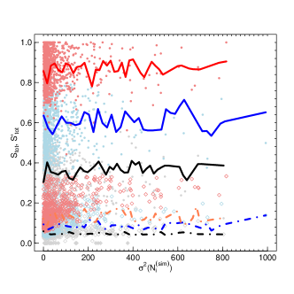From the differential and cumulative histograms shown in the plots in Figure 1, it is evident that the normal score $S_{\mathrm{tot}}$ (filled bars) spans the whole range $[0,1]$ with the values of the extremely correlated simulated clusterings ranging from 0.6 to 1, the moderately correlated with scores values between $\sim 0.4$ and 0.7, and weakly correlated clusterings have values of the total normal scores smaller than 0.5. In the same plots, the values of the total weighted scores $S^{{}^{\prime}}_{\mathrm{tot}}$ (dashed bars) are consistently smaller than $S_{\mathrm{tot}}$ and are not normalized to unity (as remarked in Sec. 2.3). The weighted total scores $S^{{}^{\prime}}_{\mathrm{tot}}$ for the three families of simulated clusterings are separated less clearly than in the case of the normal total scores, as the weights depend on the sizes of the clusters $N_{i}^{(\mathrm{sim})}$ and, consequently, the total value of the score depends on their variance $\sigma^{2}(N_{i}^{(\mathrm{sim})})$ of the sizes of the clusters. Even so, the strongly correlated clusterings are associated with values of $S^{{}^{\prime}}_{\mathrm{tot}}$ on average larger than the $S^{{}^{\prime}}_{\mathrm{tot}}$ values for partially correlated simulated clusterings and randomly drawn clusterings. The four plots in Figure 2 show that the values of the scores do not show significant dependencies over any of the four parameters describing the simulated clusterings: $N_{\mathrm{tot}}^{(\mathrm{sim})}$, $N_{\mathrm{clust}}^{(\mathrm{sim})}$, $M_{L}^{(\mathrm{sim})}$ and $\sigma^{2}(N_{i}^{(\mathrm{sim})})$. The results of the simulations demonstrate that the scores as defined in this paper, are unbiased diagnostics of the degree of correlation between the distribution of observations in a clustering and the label class values.

2.4. Choice of Clustering

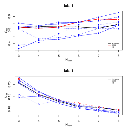
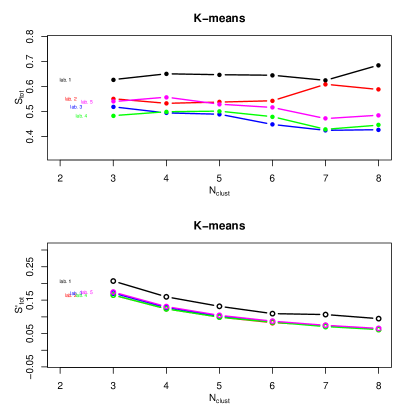
Given a label $L$ and a set of label classes $M_{L}$, CLaSPS produces distinct values of the total scores $S_{\mathrm{tot}}$ and $S^{{}^{\prime}}_{\mathrm{tot}}$ for each clustering produced by any clustering method employed (see Sec. 2.2). The clusterings produced by a single method differ for the total number of clusters $N_{\mathrm{clust}}$. The scores can be plotted as a function of the number of clusters and the clustering method, as shown in the left side of Figure 3, to identify the clusterings with the largest degree of correlation between the label classes and the clustering members. A similar plot can be used to immediately determine the clustering with the largest correlation between the features distribution of the clusters and each of the whole set of labels at once (right side plot in Figure 3).

Figure 3.— Plots of the normal and weighted total score distributions for a generic dataset for distinct total number of clusters $N_{\mathrm{clust}}$ of the clustering and type of unsupervised clustering algorithm used to produce the clusterings. Left: the total scores distributions, evaluated for a specific label $L$, are plotted as a function of the total number of clusters of the clusterings for all unsupervised clustering algorithms; right: both total score distributions are plotted as a function of the total number of clusters $N_{\mathrm{clust}}$ of the clusterings for multiple labels. In both plots, the total normal scores $S_{\mathrm{tot}}$ and weighted scores $S^{{}^{\prime}}_{\mathrm{tot}}$ are plotted separately for the sake of clarity.

Since the total scores are averaged over all the clusters in a given clustering, they can only provide information on the global degree of correlation of the distribution of label classes and the clustering membership. Information about the local correlations is carried by the value of the scores for each cluster contained in the clustering separately.

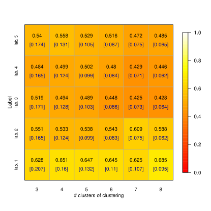
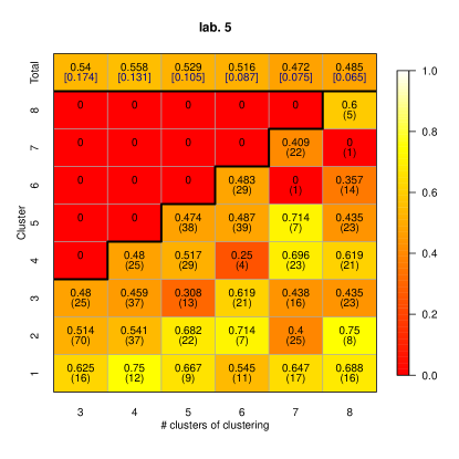
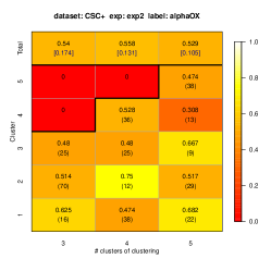
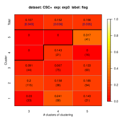
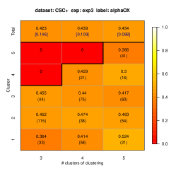
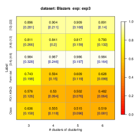
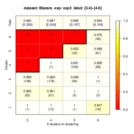
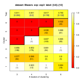
For a given label $L$ and a set of clusterings produced by the same clustering algorithm but with different number of clusters, the values of the scores and the number of members of each cluster is shown in the “heatmap” plot on the right side of Figure 4. This specific type of plot is useful to select large cluster score values that may not be reflected in the global scores, which are averaged over all clusters of the clustering (see equations (15) and (16)). The left side plot in Figure 4 shows the values of the total normal and weighted scores for distinct clusterings produced by a given clustering method as a function of the total number of clusters $N_{\mathrm{clust}}$, for a whole set of labels. These plots can be used to determine whether multiple labels show similar trends in their degrees of correlation with the distribution of members of the clusters of each clustering. In this way, correlated attributes can be selected on the basis of the result of the clustering and labeling procedure and their dependences can be taken into account during the interpretation of the results.

Figure 4.— Example of “heatmap” plots for a generic dataset and set of clusterings extracted using a given clustering method for one set of labels and one particular label class distribution. Left: each cell represents a whole distinct clustering obtained using a given clustering algorithm, and the value $S_{\mathrm{tot}}$ and $S_{\mathrm{tot}}^{{}^{\prime}}$ (in square brackets) of the total normal and weighted scores respectively are reported for a set of labels. Right: each cell (except for the cells in the upper row) represents a cluster and contains the cluster score value and the number of members of the cluster (in parentheses). The upper row shows the total normal and weighted (in square brackets) score values of each clustering.

2.5. Uncertainties

The uncertainty on the features of a dataset can affect the result of the clustering and the selection of correlations among the cluster distributions and the labels. The clustering methods discussed in Sec. 2.2 do not take into account the presence of uncertainties on the attributes. The effect of the errors on the features can be evaluated by applying CLaSPS to multiple realizations of the same dataset obtained by “perturbing” the features distribution and evaluating the spread of the scores distribution relative to the different clusterings.

In the case of the experiments described in this paper, multiple realizations of the dataset feature distributions have been obtained by assuming that the error $\sigma_{\mathrm{x_{i}}}$ on the $i$-th feature $x_{i}$ can be interpreted as the standard deviation of a normal error distribution. While this is a reasonable assumption for the uncertainties on the photometric quantities from large area surveys like the SDSS (e.g., Fukugita et al., 1996) from which the features of the datasets discussed in this paper have been extracted, this method is general. For example, if the uncertainties on distinct features have to be modeled with distinct distributions, the perturbations can be independently extracted for every single feature, according to the same procedure described in the following for gaussian distributions. For the experiments discussed in this paper we randomly extracted a distinct perturbing number $p_{i}$ from a gaussian distribution centered around zero and with width equal to twice the uncertainty $\sigma_{x_{i}}$ on the value of the attribute $x_{i}$, for any given source of the dataset. The new realization of the $i$-th feature $x_{i}$ is defined as follows:

$$x_{i}\!\rightarrow\!x^{{}^{\prime}}_{i}\!=\!x_{i}\!+\!p_{i}$$ (17)

where $p_{i}$ can be positive or negative: $p_{i}\!\in\![-\sigma_{\mathrm{x_{i}}},\!\sigma_{\mathrm{x_{i}}}]$. This approach, in general, can be time-consuming as it requires CLaSPS to be run multiple times on slightly different realizations of the same multi-dimensional features distribution. However, the high dimensionality of the feature space where clustering methods are applied usually guarantees that the results of the clustering are robust. This statement can be verified by observing the distribution of total and cluster scores values for several distinct realizations of the dataset obtained by perturbing the values of the features as described above (see Figure 5 for an example of the distribution of the values of the clusters and total scores distributions for 50 realizations obtained with the above procedure).

Figure 5.— Total scores $S_{\mathrm{tot}}$ and $S^{{}^{\prime}}_{\mathrm{tot}}$ distributions for 50 realizations of the features of a generic dataset, as described in Sec. 2.5 (solid points). In the upper panel, the cluster and total normal scores distributions for 4 distinct clusters and their clustering are plotted in full and open points respectively. In the lower panel, the weighted total scores for the same clusterings are plotted. The $\pm 5\%$ and $\pm 10\%$ intervals around the mean values of the total and clusters scores are drawn for reference in both panels. The variations of the cluster normal scores can reach 10% of their unperturbed values (open circles in the upper panel), but the variations in the total normal and weighted (solid circles in upper and lower panels) scores barely reach 5% of their values. This fact shows the robustness of the total scores values relatively to the presence of uncertainties on the features.

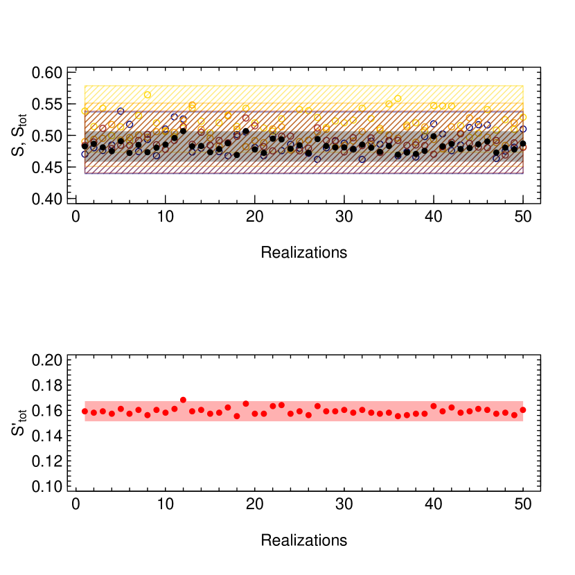
In the case of the datasets discussed in this paper and described in Sec. 3 and 4, arbitrary thresholds of 5% and 10% variation over the mean value of each total and cluster scores respectively have been set to evaluate the stability of the clusterings. The results obtained confirmed that all clusterings are insensitive to the “perturbations” to the values of the features within these values of the threshold. This result was expected, since the datasets considered in this paper are sparse in the feature space where the clustering methods are applied, leading to intrinsically stable clustering configurations.

3. Application to the CSC+ dataset

The CSC+ is an example of the class of inhomogeneous datasets that have become common thanks to the emerging VO technology. As discussed in Sec. 1, KD methods can improve the extraction of useful correlations from such samples, by minimizing the influence of biases and selection effects inherent to federated data. In this specific case, we will show that the application of the CLaSPS method leads to the determination of simple well known relations between observables from distinct spectral regions.

3.1. The CSC+ dataset

CSC+ is a sample of spectroscopically selected optical quasars with X-ray observations in the Chandra Source Catalog (Evans et al., 2010) (CSC) for which additional multi-wavelength photometric data are available. These sources have been classified as quasars using the Sloan Digital Sky Survey (Aihara et al., 2011) (SDSS) spectroscopic observations. In addition, the sources of the CSC+ sample have been selected so that both near-infrared and ultraviolet photometric observations can be retrieved from the UKIRT Infrared Deep Sky Survey (Lawrence et al., 2007) (UKIDSS) and the Galaxy Evolution Explorer (Martin et al., 2005) (GALEX) catalogs respectively.

The GALEX and UKIDSS counterparts to the sources and upper limits in both the CSC and SDSS surveys have been determined using pre-selected crossmatched catalogs containing all sources detected in the SDSS and in each of the two datasets discussed. More specifically, we have used the SDSS-GALEX crossmatched sample of sources (Budavári et al., 2009) to determine the UV counterparts of the SDSS-Chandra sources, and the crossmatched table of the UKIDSS counterparts of the SDSS stellar sources for the IR photometry, available through the web interface to the GALEX database.

The total number of sources of the CSC+ sample is 112 when considering only detection in the CSC (dataset used in experiments 1 and 2 of Table LABEL:tab:featureslabels1) and 192 including all sources with reliable Chandra upper limits for the flux in the Broad Chandra energy band as returned by the CSC sensitivity map service (dataset used in experiment 3). The final CSC+ sample is composed of radio-quiet quasars, except for two sources that can be found in the VLA FIRST Survey Catalog (Becker et al., 1995). More details on the specific data used to build the set of features and labels of the CSC+ sample described above and listed in Table LABEL:tab:featureslabels1 are discussed below.

CSC, the Chandra Source Catalog (Evans et al., 2010) includes $\sim\!1.06\times 10^{5}$ unique unresolved or slightly extended X-ray sources with 5-band photometry. The total cumulative sky coverage is 320 deg², but since the majority of sources have broad band fluxes of $\sim$10-14 cgs, the effective coverage is $\sim$260 deg². The sensitivity varies in different regions. A catalog containing CSC-SDSS positionally cross-matched sources(Evans et al., 2010) covers $\sim$133 deg², including $\sim$ 1.7$\times 10^{4}$ Chandra sources, of which $\sim$9000 have stellar and $\sim$7800 extended optical counterparts, mostly galaxies.

SDSS DR8 (Aihara et al., 2011) has observed $\sim\!1.4\times 10^{4}$ deg² of the sky in 5 bands ugriz, with photometric limiting magnitude of 22.2 in the r band (95% completeness for point sources). It includes spectra of $\sim\!1.8\!\times$10⁶ sources in the 380-920 nm wavelength range. Classification in quasar, high-redshift quasars, galaxy, star and late-type stars classes and spectroscopic redshifts are available for these spectroscopically observed sources, based on the measured lines of the optical spectra. If emission lines are observed and if the source has a final redshift larger than 2.3, it is classified as a high-redshift quasars.

UKIDSS (Lawrence et al., 2007) has been designed to be the infrared counterpart to the SDSS and covers $\sim$7500 deg² of the sky in JHK near-infrared bands to K=18.3. The Large Area Survey (LAS) has imaged $\sim$ 4000 deg² (overlapping with the SDSS), with the additional Y band to a limiting magnitude of 20.5. The final area of the overlap between CSC and UKIDSS LAS will be $\sim$50 deg².

GALEX (Martin et al., 2005) is a 2-band survey (far and near UV) that has observed the whole sky up to a limiting magnitude $\emph{nuv}\!=\!20.5$. It includes deep fields to magnitude 25 with spectroscopic observations.

3.2. CSC+ dataset: features and labels

Three different experiments have been performed on the CSC+ sample using distinct combinations of features for the clustering and labels for the evaluation of the scores. The features have all been extracted from the overall set of colors obtained from consecutive photometric filters, while the labels are either photometric measurements (not used for the clustering, in these cases) or the spectroscopic redshifts, classification flags and other parameters related to the shape of the spectral energy distributions of the sources. For example, the $\alpha_{OX}$ parameter (Avni & Tananbaum, 1982) has been used as a label. The $\alpha_{OX}$ parameter measures the relative amount of energy emitted in the optical and X-rays and is defined as the spectral slope between the optical/UV and X-rays monochromatic luminosities at $\mathrm{E}\!=\!2$ KeV and $\lambda\!=\!2500$ Å respectively:

$$\alpha_{OX}\!=\!-\frac{\log{(\nu L_{\mathrm{\nu}})}_{\mathrm{Opt}}\!-\!\log{(\nu L_{\mathrm{\nu}}})_{\mathrm{X}}}{\log{(\nu_{\mathrm{Opt}})}\!-\!\log{(\nu_{\mathrm{X}}})}\!+\!1$$ (18)

The features of the experiments performed using the CSC+ sample are described in detail in Table LABEL:tab:featureslabels1.

Table 3List of the experiments performed on the CSC+ sample. A short description of dataset, the number of sources of the dataset, the total number of clusters for the clustering produced and the list of features and labels used are provided for each experiment. In the Labels column, each label is followed, in curly brackets, by the binning used to evaluated the scores. For categorial labels, the binning is specified by providing the actual values corresponding to the distinct classes; for continuous labels, the extremes of the bins defining the classes are provided.

Experiment	Dataset	# sources	# clusters	Features	Labels
Exp. 1	SDSS quasars with	112	{3, 4, 5}	$fuv$-$nuv$,$nuv$-$u$,$u$-$g$,	$z_{\mathrm{spec}}${0.4,1.1,1.9},$HR(ms)${-0.4,-0.2,0},
	CSC detection			$g$-$r$,$r$-$i$,$i$-$z$,$z$-$Y$,	$HR(hm)${-0.1,0,0.2},
				$Y$-$J$,$J$-$H$,$H$-$K$	$L(B)${2,4,6,8}$\times 10^{43}$ erg s-1,
					$\alpha_{\mathrm{OX}}${1.3}
Exp. 2	SDSS quasars with	112	{3, 4, 5}	$fuv$-$nuv$,$nuv$-$u$,$u$-$g$,	$z_{\mathrm{spec}}${0.4,1.1,1.9},
	CSC detections			$g$-$r$,$r$-$i$,$i$-$z$,$z$-$Y$,	$\alpha_{\mathrm{OX}}${1.3},
				$Y$-$J$,$J$-$H$,$H$-$K$,	$L(B)${2,4,6,8}$\times 10^{43}$ erg s-1
				$HR(ms)$,$HR(hm)$
Exp. 3	SDSS quasars with	192	{3, 4, 5}	$fuv$-$nuv$,$nuv$-$u$,$u$-$g$,	$z_{\mathrm{spec}}${0.4,1.1,1.9},
	CSC detections and			$g$-$r$,$r$-$i$,$i$-$z$,$z$-$Y$,	$\alpha_{\mathrm{OX}}${1.3},$f_{\mathrm{Xdet}}${0,1}
	upper limits			$Y$-$J$,$J$-$H$,$H$-$K$	$L(B)${2,4,6,8}$\times 10^{43}$ erg s-1

3.3. Results of the application of CLaSPS to CSC+

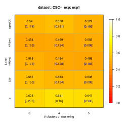
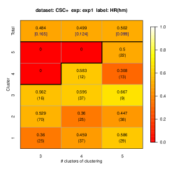
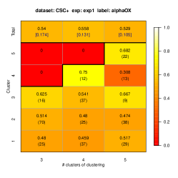
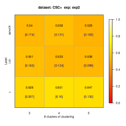
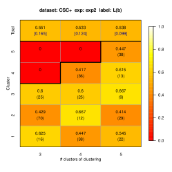
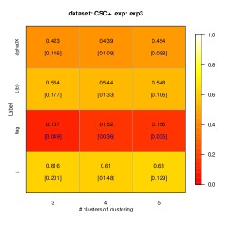
The main results of the application of CLaSPS to the two different datasets based on the CSC+ sample are summarized in the plots in Figures 7 and 6.

In the first experiment (see Table LABEL:tab:featureslabels1), we have found a significant correlation between the near-infrared, optical and ultraviolet colors, used as features, and the $\alpha_{\mathrm{OX}}$ index for two clusterings, composed of 4 and 5 clusters respectively and produced using the K-means and SOM methods (see leftmost plot in the upper row of Figure 6). Even if the total normal and weighted scores values for the clustering composed of 5 total clusters are smaller than the scores for the other two clusterings, this clustering has been considered more interesting because of the larger number of sources contained in clusters with significantly large values of the cluster scores. We will discuss here the correlation involving the members of the second, third and fourth clusters of the clustering composed of five total clusters (see upper-left plot in Figure 6).

Figure 6.— Results of the application of the CLaSPS method to the datasets based on the CSC+ sample (for details see Sec. 3). In the upper row, plots from the Exp.1 are shown. From left to right: total scores distribution for the clusterings obtained with the K-means method; cluster scores distribution for the label X-ray hardness ratio $HR(hm)$; cluster scores distribution for the $\alpha_{\mathrm{OX}}$ index. The right plot, in particular, has been discussed extensively in Sec. 3.3. In the central row, plots from the results of Exp.2 are showed. From left to right: total scores distribution for the clusterings obtained with the K-means method; cluster score distribution for the total X-ray luminosity used as label; cluster scores distribution for the $\alpha_{\mathrm{OX}}$ index. In the lower row, the plots from the Exp.3 are shown. From left to right: total score distributions of the clusterings obtained using the SOM method; cluster scores distribution for the label represented by the X-ray detection flag; cluster scores distribution for the $\alpha_{\mathrm{OX}}$ index (for more details, see Sec. LABEL:tab:featureslabels1). The discussion in Sec. 3.3 and Figure 7 are based on the clustering with five total clusters of the second experiment (mid-left plot in this figure), using as label the $\alpha_{\mathrm{OX}}$ spectral index.

In order to determine whether there is a subset of features responsible for the correlation observed, a Principal Component Analysis (Hartigan, 1975) (PCA) has been performed on the feature distribution of these three clusters. The PCA finds that the correlation is mostly due to the blue optical/UV colors $nuv-u$ and $u-g$.

The correlation between the optical blue and near-UV features of quasars and the $\alpha_{\mathrm{OX}}$ spectral index has been discussed in several papers in the literature (see, for example Vignali et al., 2003; Lusso et al., 2010), and can be explained on the basis of the definition of the $\alpha_{\mathrm{OX}}$ spectral index itself (given in Sec. 3.2), and the characteristics of the spectral energy distributions (SED) of homogeneous samples of radio-quiet quasars observed in the X-rays. In particular, the presence of this correlation is usually associated with the presence of a prominent component of the SED of the quasars at near-UV wavelengths, called “big-blue-bump”.

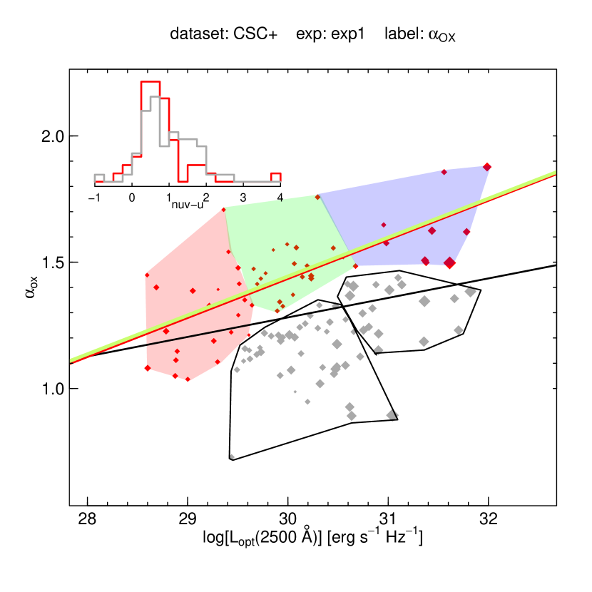
In Figure 7, we show the $L_{\mathrm{opt}}(2500\AA)$ vs $\alpha_{\mathrm{OX}}$ distribution of the sample used in the first experiment for the clustering composed of five clusters. The projections of the five clusters are plotted as shaded colored regions and closed black lines for the three clusters with large score values (clusters one, three and five in the upper-right plot in Figure 6) and the remaining two clusters (clusters two and four in the upper-right plot in Figure 6) respectively.

The clusters with large scores are those for which the correlation between the optical mono-chromatic luminosity and the $\alpha_{\mathrm{OX}}$ index is more significant. In fact, while the significance of finding a correlation between the two parameters for the whole sample is low ($\sim 43\%$), the significance is larger for the subset of points of the three clusters selected ($\sim 90\%$). In Figure 7, the size of the symbols are proportional to $nuv-u$ color values of the sources, and it is evident that the members of the correlated clusters have, on average, lower values of $nuv-u$. This suggests that the SEDs of the sources belonging to the three clusters with large scores values are dominated by the “big blue bump” component (the red and black lines are associated with the best fitting linear relations for the members of the three clusters and the total sample respectively, and are shown only for reference). In this regard, we conclude that, despite the fact that the CSC+ sample used for this experiment is highly inhomogeneous, CLaSPS select a subset of clusters whose members show a significant degree of correlation between the optical mono-chromatic luminosity $L_{\mathrm{opt}}(2500\AA)$ and the $\alpha_{\mathrm{OX}}$ spectral index. The behavior of this subset of sources, is in agreement with the results found and discussed in literature for homogeneously drawn samples of X-ray emitting radio-quiet optically selected quasars.

Figure 7.— Distribution of the sources in the first experiment (Exp. 1) with the CSC+ sample in the $L_{\mathrm{opt}}(2500\AA)$ vs $\alpha_{\mathrm{OX}}$ plane. The shaded regions containing the red symbols correspond to the projections of the three clusters (clusters one, three and five shown in the upper-right plot in Figure 6) with large scores values for the label $\alpha_{\mathrm{OX}}$ in the first experiment (Exp. 1 in Table LABEL:tab:featureslabels1). The two black polygons represent the projections of the remaining two clusters (clusters two and four in the mid-left heatmap in Figure 6) with small scores values. The size of the symbols used for the plots is proportional to the near-ultraviolet color $nuv-u$ of each source, and in the inset of the plot the histograms of the $nuv-u$ color distribution for sources belonging to the three interesting clusters and the two unselected clusters is shown. The red and black lines represent the linear regression for the points in the correlated clusters and the whole sample, respectively. The red line is in perfect agreement with the best-fit relation from (Lusso et al., 2010) (green line), derived from a sample of 545 AGNs.

A similar correlation pattern, weaker than the one observed for the $\alpha_{\mathrm{OX}}$ index though, is observed in the distribution of score values for the hardness ratio $HR(hm)$ used as label (see central plot of the upper row in Figure 6).

In the second experiment (Exp. 2 in Table LABEL:tab:featureslabels1), the hardness ratios $HR(hm)$ and $HR(ms)$ have been used as features, together with the other variables used as features in the first experiment. Correlations similar to those observed in the first experiment are observed for in the clusterings with 4 and 5 total clusters each in the second experiment (see central and left plots of the central row in Figure 6).

The PCA of the feature distribution of the clusters with larger values of the scores showed that the correlation can be mostly attributed to a subset of features including the $nuv-u$ and $u-g$ colors and both the X-rays hardness ratios.

In the third experiment (Exp. 3 in Table LABEL:tab:featureslabels1), we have used as label the values of upper limits for X-ray luminosity and considered them as detections in order to test whether the distribution of not-X-ray colors of the sample correlates with either the detections or the upper limits observed in X-rays. As shown in the plots of the lower row in Figure 6, no interesting correlations among the set of features and the labels considered is visible. In particular, the X-ray detection flag is not correlated with the near-infrared, optical and ultraviolet colors used as features, regardless of the clustering methods and total number of clusters of the clusterings.

4. Application to the Blazars dataset

CLaSPS has also been applied to a sample of blazars with available photometric data spanning from the mid-infrared to optical wavelengths, with additional information in the $\gamma$-ray spectral range. Blazars are a peculiar family of AGNs characterized by rapid variability at all frequencies. The other distinguishing observational properties of blazars include flat radio spectra, high observed luminosity and highly variable radio to optical polarization. Blazars are a dominant class of extragalactic sources at radio, microwave and $\gamma$-ray frequencies. The observational characterization of this class of galaxies is interesting as a tool to shed some light on the physical mechanisms responsible for the emission. The experiments described have aimed at the characterization of the blazars population in the infrared bands, extending the type of analysis already performed on 2MASS (Skrutskie et al., 2006) data (e.g. Chen et al., 2005) to longer wavelengths, using the recently released WISE (Wright et al., 2010) mid-infrared photometric data.

4.1. The Blazars dataset

The Blazars sample is based on the ROMA-BZCAT (Massaro et al., 2009) list of blazars. This catalog assembles blazars known in the literature and confirmed by the inspection of their multi-wavelength emission. The members of the ROMA-BZCAT catalog are selected on the basis of a set of criteria involving the presence of detection in the radio band down to 1 mJy flux density at 1.4 GHz (2.1 $\mu m$), the optical identification and availability of an optical spectrum for further spectral classification and the detection of isotropic X-ray luminosity $L_{X}\geq 10^{43}$ erg $\times s^{-1}$. Such criteria do not yield a statistically homogeneous or complete sample of blazars but provide the largest and more carefully selected sample of confirmed blazars available to date. In the ROMA-BZCAT, blazars are also divided in three spectral classes, based on the prominence of the emission features in the optical spectra of these sources: BZB for the BL Lac sources, i.e. AGNs with featureless optical spectra and narrow emission lines; BZQ for flat-spectrum radio quasars with optical spectra showing broad emission lines and typical blazars behavior; BZU for blazars of uncertain type, associated with sources with peculiar characteristics but also showing typical traits of the blazars (a more detailed description of on the Blazars sample can be found in (Massaro et al., 2011; D’Abrusco et al., 2012)). This sample includes $\sim 800\ \gamma$-ray sources from the 2FLG Nolan et al. (2012) associated with members of the catalog to a high level of confidence, and 571 of these blazars are also present in the ROMA-BZCAT. More details on the specific data used as features and labels of the Blazars sample can be found below (for SDSS data, see Sec. 3.1).

2MASS (Skrutskie et al., 2006) has uniformly scanned the whole near-infrared sky in three bands $H$, $J$ and $K_{s}$ detecting points sources brighter than $\sim 1$ mJy in each filter, with with positional accuracy of $0.4^{\prime\prime}$, to a magnitude limit (for stellar sources in unconfused regions and outside of the galactic plane) of 15.8 in the $J$ band;

The WISE mission (Wright et al., 2010) has observed the entire sky in the mid-infrared spectral interval at 3.4, 4.6, 12, and 22 $\mu$m with an angular resolution of 6.1^′′, 6.4^′′, 6.5^′′ & 12.0^′′ in the four bands, achieving 5$\sigma$ point source sensitivities of 0.08, 0.11, 1 and 6 mJy in unconfused regions on the ecliptic, respectively. The astrometric accuracy of WISE is $\sim 0.50^{\prime\prime},0.26^{\prime\prime},0.26^{\prime\prime}$, and 1.4^′′ for the four WISE bands respectively.

The 2FLG catalog (Nolan et al., 2012) contains primarily unresolved sources detected in the all-sky Fermi observations obtained throughout the second year of operation. The sources, after detection and the localization in the sky, are assigned, among other parameters, an integrated flux in the 100 MeV to 100 GeV energy range, a spectral shape and a significance parameter TS based on how significantly each source emerges from the background. Only sources with TS $\geq$ 25, corresponding to a significance of $4\sigma$, have been included in the catalog. Each of the 1873 2FLG sources have been considered for identification with already known astronomical sources available in literature multi-wavelength observations. For 127 of the 2FLG sources firm identifications have been produced (namely, reliable identifications based on synchronous periodic variability of the sources, coincident spatial morphologies for extended sources or correlated aperiodic variability). The remaining sources have been investigated for association with sources contained in a list of source catalogs based on different multi-wavelength observations. The BZCAT (Massaro et al., 2009) catalog is one of the catalogs used for the association of the 2FLG sources, and 571 2FGL sources have been associated with a BZCAT blazar. The $\gamma$-ray detection flags used in the experiments described in this paper are based on the official associations of the 2FLG sources from (Nolan et al., 2012).

4.2. Blazars dataset: features and labels

In the first experiment, we have used as features the colors calculated with consecutive filters from mid-infrared (WISE) to the optical (SDSS). As labels, we have used the spectroscopic classification in BZB, BZQ and BZU from the ROMA-BZCAT catalog (Massaro et al., 2009), the radio flux density at the frequency $\nu=1.4$ GHz and a $\gamma$-ray detection flag. Such flag is equal to 1 for the ROMA-BZCAT sources than have been associated with a $\gamma$-ray source from 2FGL catalog (Nolan et al., 2012), and 0 for all the other sources.

In the second experiment, the labels used for the first experiment Exp. 1 in Table LABEL:tab:featureslabels2 have been complemented by WISE colors, not used as features in this case, while the Fermi detection flags have not been used as label because this sample is composed of all the blazars of our sample associated with Fermi detections. In the third experiment, only the optical and near-infrared colors from SDSS and UKIDSS respectively have been used as features, while the WISE mid-infrared colors and the Fermi detection flag have been added to the set of labels already used in the first experiment for all blazars, regardless of their association with Fermi detections. The parameters of the two experiments are shown in details in Table LABEL:tab:featureslabels2.

Table 4Characteristics of the experiments performed on the Blazars sample. For a detailed description of the columns, refer to the caption of the Table LABEL:tab:featureslabels2.

Experiment	Dataset	# sources	# clusters	Features	Labels
Exp. 1	BZCAT blazars with	241	{3, 4, 5, 6}	$u$-$g$,$g$-$r$,$r$-$i$,	source class{BZB, BZQ, BZU},
	FIR, NIR and Optical			$i$-$z$,$z$-$J$,$J$-$H$,	$f(1.4\mathrm{GHz})${103,3$\times 10^{3}$}
	photometry			$H$-$K$,$K$-$[3.4]$,$[3.4]$-$[4.6]$,
				$[4.6]$-$[12]$,$[12]$-$[22]$
Exp. 2	$\gamma$-ray detected	241	{3, 4, 5, 6}	$u$-$g$,$g$-$r$,$r$-$i$,	source class{BZB, BZQ, BZU},
	BZCAT blazars with			$i$-$z$,$z$-$J$,$J$-$H$,	$f(1.4\mathrm{GHz})${103,3$\times 10^{3}$},
	FIR, NIR and Optical			$H$-$K$,$K$-$[3.4]$,$[3.4]$-$[4.6]$,
	photometry
Exp. 3	BZCAT blazars with	241	{3, 4, 5, 6}	$u$-$g$,$g$-$r$,$r$-$i$,	source class{BZB, BZQ, BZU},
	NIR and Optical			$i$-$z$,$z$-$J$,$J$-$H$,	$f(1.4\mathrm{GHz})${103,3$\times 10^{3}$},
	photometry			$H$-$K$	$f_{\mathrm{\gamma det}}${0,1},$[3.4]$-$[4.6]${0,0.5,1,
					1.5,2},$[4.6]$-$[12]${0,1,2,3,4,5},
					$[12]$-$[22]${0,1,2,3,4}

4.3. Results of the application of CLaSPS to Blazars dataset

The results of the application of CLaSPS to the three experiments based on the Blazars sample and described in Table LABEL:tab:featureslabels2 are shown in the plots in Figure 8.

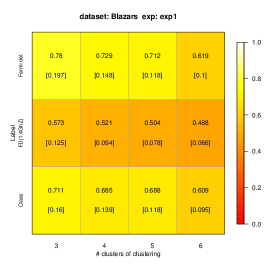
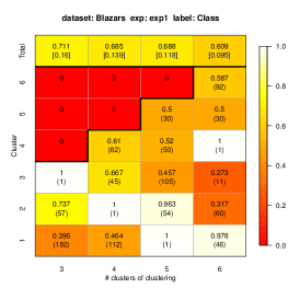
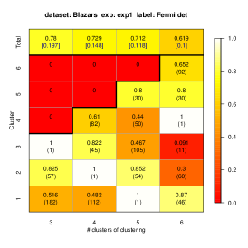
The main conclusion that can be drawn from the results of the first experiment (plots in the upper row in Figure 8), is that the distribution of blazars in the optical+near-infrared+mid-infrared colors feature space, consistently throughout the distinct clustering methods, strongly correlates with the spectral classification of the Blazars. The correlation is noticeable, based on the large values of the total normal and weighted scores evaluated using the blazars spectral class as label for all clustering (upper-mid plot in Figure 8). In particular, the largest total normal and weighted score values for this label are both obtained for the clustering with total three clusters and produced with the K-means algorithm (upper-mid plot in Figure 8).

Figure 8.— Results of the application of the CLaSPS method to the datasets based on the Blazars sample (for details see Sec. 4). In the upper row, plots from the Exp.1 are shown. From left to right: total scores distributions for clustering obtained with the K-means method; cluster scores distributions for the spectral class of the blazars used as label; cluster scores distributions for the $\gamma$-ray detection flag used as label. In the lower row, plots from the results of Exp.3 are shown. From left to right: total score distributions for clusterings created by the K-means method; cluster scores distribution for the $[3.4]-[4.6]$ WISE color used as label; cluster scores distribution for the $[4.6]-[12]$ WISE color used as label.

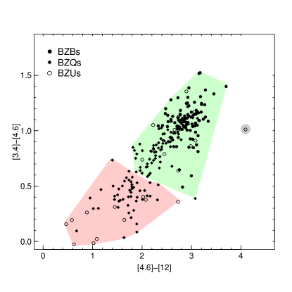
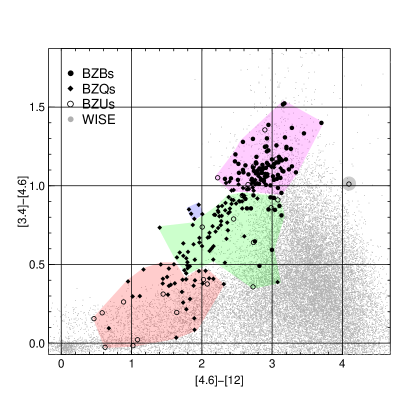
In order to verify whether there is a smaller subset of features responsible for the correlation, a PCA was carried out on the feature distribution of the two clusters with more than one member, of the clustering with three total clusters produced by the K-means with the (BZB, BZQ, BZU) spectral classes used as labels. This analysis has shown that the spectral classification of the sources of the Blazars sample correlates very strongly with the mid-infrared colors from WISE. The projection of the feature space distribution of the sources in the Blazars sample onto the WISE $[4.6]-[12]$ vs $[3.4]-[4.6]$ color-color space is shown in the left plot in Figure 9. In this plot, the sources are plotted with different symbols according to the value of the label, the spectral class (BZB, BZQ or BZU), and the three regions occupied by the projections of the three clusters of the clustering with total three clusters are represented as shaded colored areas. This finding has been discussed in detail in (Massaro et al., 2011), where an explanation of the new correlation has been proposed, in terms of the currently accepted emission mechanisms of blazars.

The same correlation between the distribution of features of the clusterings and the spectral classification has been observed in the second experiment. In this case, the dataset used contains only blazars from the ROMA-BZCAT catalog which have been associated with $\gamma$-ray sources in the 2FLG (Nolan et al., 2012). Similarly at what found for the second experiment (Exp. 2 in Table LABEL:tab:featureslabels2), the correlation can be almost entirely ascribed to the peculiar WISE colors distribution of the blazars.

An even stronger correlation has been observed in the third experiment. The third experiment has involved the same dataset used in the first experiment, comprising blazars from the BZCat with optical and near-infrared colors as features and the WISE infrared colors $[3.4]-[4.6]$, $[4.6]\!-\![12]$ and $[12]\!-\![22]$ as labels instead. The three WISE colors, used as labels, have been binned as shown in Table LABEL:tab:featureslabels2.

The lower central and left plots in Figure 8 show the scores values distributions for the clusterings produced by the K-means method on the third experiment (Exp. 3 in Table LABEL:tab:featureslabels2) calculated using as labels the two colors $[3.4]\!-\![4.6]$ and $[4.6]\!-\![12]$ from WISE. The large values of the scores for all clusterings indicate that a strong correlation exists between the distribution of sources in the clusterings and their mid-IR colors. Based on the binning used in this experiment for these two labels (see Table LABEL:tab:featureslabels2), this result suggests that the distribution of blazars in the mid-infrared colors is peculiar, as most blazars are contained in a narrow region of the mid-IR WISE colors space.

This fact is evident in the right plot of Figure 9, where the projection onto the WISE $[3.4]\!-\![4.6]$ vs $[4.6]\!-\![12]$ color-color plane of the distribution of the blazars in the feature space of the third experiment (Exp. 3 in Table LABEL:tab:featureslabels2) is shown. The regions occupied by the projections of the clusters of the clustering with five total clusters produced by the K-means algorithm (see lower central and left plots in Figure 8) are represented by shaded colored areas. The symbols of the points, as in the left plot in Figure 9, reflect the spectral classification. The horizontal and vertical black lines correspond to the bin limits of the bins used for the $[3.4]\!-\![4.6]$ and $[4.6]\!-\![12]$ WISE colors used as labels (see Table LABEL:tab:featureslabels2 for more details about the experiment). The clusters in this plot are associated with the values of the total and cluster scores shown in the column corresponding to the clustering with total five clusters in both the lower central and left plots in Figure 8, for the two WISE colors respectively. The red, green and magenta large regions correspond to the second, third and fifth clusters of the clustering respectively, while the small five-members group corresponds to the first cluster and the single-source cluster is the fourth cluster in the two plots of Figure 8. Multiple generic sources from the WISE catalog, drawn from a region of the sky at high galactic latitude, are plotted as small gray points to show that the locus occupied by the blazars is clearly separated from the high-density regions of the overall distribution of WISE sources in the same color-color plane.

In this case, the application of CLaSPS has helped to determine a previously unknown correlation between a class of astronomical sources and a small number of features, as the clusters of all clusterings follow a narrow locus in the WISE $[3.4]-[4.6]$ vs $[4.6]-[12]$ color-color plane, occupied by the whole sample of blazars. While this pattern is clearly visible also in the low-dimensional two/three dimensional distribution of the blazars WISE colors, it has been discovered during the exploration of the multi-dimensional feature space generated by the multi-wavelength color of BZCat blazars. This is an example of low-dimensional pattern that had gone, so far, unnoticed and that a general method for the determination of correlations in complex feature spaces, like CLaSPS, has helped to single out and characterize further.

A thorough investigation of the spectral mid-infrared and $\gamma$-ray properties of this sample of blazars that result in this peculiar pattern, has been presented in (D’Abrusco et al., 2012). Some of the authors of this paper have also developed a method, based on the mid-infrared properties of BZCat blazars discussed above (Massaro et al., 2012), for the selection of blazars candidates from WISE photometric data.

Figure 9.— Left plot: projection of the distribution in the multi-dimensional feature space of the Blazars sample used in the first experiment (Exp. 1 in Table LABEL:tab:featureslabels2) onto the $[4.6]\!-\![12]$ vs $[3.4]\!-\![4.6]$ $\mu$m WISE color-color plane. Blazars of different spectral classes (BZB, BZQ and BZU) according to the BZCat are plotted with different symbols. The shaded regions correspond to the projections of the three clusters of the clustering with three total clusters obtained with the K-means algorithm using the spectral class as label (upper-mid plot of Figure 8). The interpretation of the clustering is discussed in Sec. 4.3. Right plot: plot of the distribution of the Blazars sample used in experiment three (Exp. 3) in the WISE color-color plane generated by the colors $[4.6]\!-\![12]$ and $[3.4]\!-\![4.6]$, used as labels. The horizontal and vertical black lines represent the edges of the label bins used in the experiment three for the $[3.4]\!-\![4.6]$ and $[4.6]\!-\![12]$ WISE colors respectively (the distribution of scores associated with these two labels are shown in the lower central and left plots in Figure 8). The background grey dots are shown for reference and correspond to 453420 WISE generic sources detected at high Galactic latitude. This plot has been adapted from a similar plot in (D’Abrusco et al., 2012).

5. Summary and future developments

In this paper we have presented CLaSPS, a new method for the determination of correlations in complex astronomical datasets, based on KD techniques for unsupervised clustering supplemented by the use of external information to label and characterize the content of the clusters (Sec. 2). We have introduced the score (Sec. 2.3) and shown the reliability of the score as a measure of the degree of correlation among the membership distribution of sources in a clustering and the distribution of a quantitative or categorial label in distinct classes, using simulated clusterings (Sec. 2.4).

We have also discussed the applications of CLaSPS to two different samples composed of extragalactic sources with multi-wavelength photometry used as features: the first dataset, CSC+ (Sec. 3), is composed of spectroscopically confirmed quasars from the SDSS DR8 with multi-wavelength observations in the near-infrared, optical and ultraviolet, and detected (or with reliable upper limits) in the Chandra X-ray CSC catalog; the second dataset (Sec. 4) is composed of optically confirmed blazars with mid-infrared, near-infrared and optical observations, complemented, for a subset of the sources, by $\gamma$-ray data from the 2FGL.

The main result of the application of CLaSPS to the CSC+ dataset has been the confirmation of a well known correlation (see, for example Lusso et al., 2010) between the near-ultraviolet/blue optical luminosity of optically selected radio-quiet quasars and the spectral index $\alpha_{\mathrm{OX}}$ (Sec. 3.3) in a subset of the highly inhomogeneous CSC+ sample. CLaSPS has narrowed the CSC+ sample to three specific clusters that show significant correlation between the $L_{\mathrm{opt}}(2500\AA)$ mono-chromatic luminosity and the $\alpha_{\mathrm{OX}}$ spectral index, based on the clustering of the CSC+ sample in the feature space generated by the near-infrared, optical and ultraviolet photometric data. Further analysis of the results have shown that the correlation for the subset of sources contained in the correlated clusters is driven by the values of the $nuv-u$ color, as an indicator of the presence of the “big-blue-bump” component in the SEDs of the sources.

In the case of the experiments performed on the blazars sample, CLaSPS has revealed an unknown correlations between the spectral classification of the blazars in BZQs, BZBs and BZUs (Sec. 4.1) and their distribution in the feature space generated by mid-infrared, near-infrared and optical colors. Further investigation has shown that the correlation is almost entirely attributable to the peculiar pattern followed by BZCat and $\gamma$-ray detected blazars follow in the WISE mid-infrared color space (Sec. 4.3). The implications of this pattern on the modeling of blazars emission mechanism and a novel method for the selection of candidate blazars from mid-infrared survey photometric data based on such pattern have been investigated in other works by some of the authors (Massaro et al., 2011; D’Abrusco et al., 2012; Massaro et al., 2012).

While in this paper we have described applications of CLaSPS to inhomogeneous samples obtained by federating data from general purpose large area surveys, we plan to apply the method to large homogeneous samples of extragalactic sources, like the Chandra-COSMOS dataset (Elvis et al., 2009; Civano et al., 2012).

CLaSPS selects the optimal clustering based on the scores, a measure of the correlation between the clustering membership and a given partition of one external observable used as label. For this reason, as discussed in Sec. 2.1, CLaSPS differentiate itself from “cluster ensembles” techniques. Nonetheless, three different aspects of the current CLaSPS method could be improved by the application of cluster ensembles techniques: 1) the limited number of clustering techniques used may bias the exploration of the clusterings towards particular aspects of the feature distribution of the dataset considered. Moreover, CLaSPS does not to take into account the properties and, potentially, weaknesses of each distinct clustering techniques; 2) the choice of the optimal clustering is based on a single label at the time. Correlations between a given set of clusterings and multiple labels cannot be captured by CLaSPS, but are left to the interpretation of multiple distinct label experiments; 3) the choice of the optimal clusterings in CLaSPS is based on a single “view” of the dataset, i.e. on clusterings obtained using a single set of sources and/or features.

The first point could be easily addressed by widening the portfolio of clustering methods used by CLaSPS. Then, cluster ensembles methods could be applied to subsets of clusterings (grouped by total number of clusters or by type of clustering method) to determine the “consensus clustering” of each subset of clusterings. The scores would then be evaluated on the set of consensus clusterings determined in this way. The second point could be similarly addressed by searching for the “consensus clusterings” of the set of optimal clusterings selected through the scores values for different labels.

The third point is particularly important for astronomy, because most astronomical datasets present different number of features available for different members of the dataset. In its current implementation, CLaSPS can be applied only to clusterings obtained with a fixed given subset of sources and features. CLaSPS, in this scenario, can be applied separately to distinct groups of sources in the dataset with a set of common features. In order to overcome this limitation, distinct sets of clusterings could be obtained for different “views” of the dataset, i.e. different subsets of the datasets with the same set of features available. Then, the multiple clusterings obtained with on the different views of the dataset with different clustering techniques could be consolidated into a single set of clusterings through the application of cluster ensembles technique on the groups of clustering obtained with the same clustering technique on distinct views of the dataset. This approach is similar to “features distributed clustering” and “object distributed clustering” scenarios typical of practical application of clustering ensemble (Strehl & Ghosh, 2003).

A further improvement to the CLaSPS method is related to the choice of the classes of the labels. In the frequent case of quantitative continuous labels, the choice of the binning is crucial for the evaluation of the scores and, in turn, for the determination of the correlations among features and labels, if any. While the astronomer deciding the binning of the labels on the basis of a priori knowledge of the specific topic considered is a viable option for most cases where the astronomer tries to generalize an already known correlation or a generic problem (e.g. the characterization of astronomical sources based on their photometric parameters for this paper) is investigated, this can be a limitation to the generality of the method when the aim of the experiments is a “blind” exploration of multi-dimensional astronomical datasets. In order to improve this aspect of the CLaSPS method, we are exploring the possibility of complementing the astronomer’s definition of classes of labels with spontaneous classes that can be determined from the intrinsic distribution of the labels themselves by the application of non-parametric KD techniques.

References

- Aihara et al. (2011) Aihara, H., Allende Prieto, C., An, D., et al. 2011, ApJS, 193, 29
- Avni & Tananbaum (1982) Avni, Y., & Tananbaum, H. 1982, ApJ, 262, L17
- Babu & Feigelson (2007) Babu, G. J., & Feigelson, E. D. 2007, Statistical Challenges in Modern Astronomy IV, 371
- Ball & Brunner (2010) Ball, N. M., & Brunner, R. J. 2010, International Journal of Modern Physics D, 19, 1049
- Bazarghan (2012) Bazarghan, M. 2012, Ap&SS, 337, 93
- Becker et al. (1995) Becker, R. H., White, R. L., & Helfand, D. J. 1995, ApJ, 450, 559
- Bonfield et al. (2010) Bonfield, D. G., Sun, Y., Davey, N., et al. 2010, MNRAS, 405, 987
- Borne et al. (2009) Borne, K., Accomazzi, A., Bloom, J., et al. 2009, astro2010: The Astronomy and Astrophysics Decadal Survey, 2010, 6P
- Borne et al. (2011) Borne, K. D., Stassun, K., Brunner, R. J., et al. 2011, Bulletin of the American Astronomical Society, 43, #252.09
- Budavári et al. (2009) Budavári, T., Heinis, S., Szalay, A. S., et al. 2009, ApJ, 694, 1281
- Chen et al. (2005) Chen, P. S., Fu, H. W., & Gao, Y. F. 2005, NewA, 11, 27
- Civano et al. (2012) Civano, F. et al., submitted.
- Collister & Lahav (2004) Collister, A. A., & Lahav, O. 2004, PASP, 116, 345
- Comparato et al. (2007) Comparato, M., Becciani, U., Costa, A., et al. 2007, PASP, 119, 898
- D’Abrusco et al. (2009) D’Abrusco, R., Longo, G., & Walton, N. A. 2009, MNRAS, 396, 223
- D’Abrusco et al. (2012) D’Abrusco, R., Massaro, F., Ajello, M., et al. 2012, ApJ, 748, 68
- Djorgovski & Davis (1987) Djorgovski, S. G. & Davis, M. 1987, ApJ, 313, 59.
- Elvis et al. (2009) Elvis, M., Civano, F., Vignali, C., et al. 2009, ApJS, 184, 158
- Evans et al. (2010) Evans, I. N., Primini, F. A., Glotfelty, K. J., et al. 2010, ApJS, 189, 37
- Fabbiano & Trinchieri (1985) Fabbiano, G. & Trinchieri, G. 1985 ApJ, 296, 430-457.
- Fabbiano & Shapley (2002) Fabbiano, G. & Shapley, A. 2002 ApJ, 565, 908-920.
- Freeman et al. (2009) Freeman, P. E., Newman, J. A., Lee, A. B., Richards, J. W., & Schafer, C. M. 2009, MNRAS, 398, 2012
- Fukugita et al. (1996) Fukugita, M., Ichikawa, T., Gunn, J. E., et al. 1996, AJ, 111, 1748
- Geach (2012) Geach, J. E. 2012, MNRAS, 419, 2633
- Ghosh & Acharya (2011) Ghosh, J. & Acharya, A. 2011, Cluster ensembles, in Wiley Interdisciplinary Reviews: Data Mining and Knowledge Discovery, 1, 4, 305-315, John Wiley & Sons, Inc.
- Hassan & Fluke (2011) Hassan, A., & Fluke, C. J. 2011, PASA, 28, 150
- Hartigan (1972) Hartigan, J. A. 1972, Journal of the American Statistical Association, 67, 337, 123-129.
- Hartigan (1975) Hartigan, J. A. 1975, Clustering Algorithms, Wiley, New York.
- Hastie et al. (2009) Hastie, T., Tibshirani, R., & Friedman, J. 2009, The Elements of statistical learning, Springer.
- Kohonen (1990) Kohonen, T. 1990, Proceedings of the IEEE, 78, 1464.
- Laurino et al. (2011) Laurino, O., D’Abrusco, R., Longo, G., & Riccio, G. 2011, MNRAS, 418, 2165
- Lawrence et al. (2007) Lawrence, A., Warren, S. J., Almaini, O., et al. 2007, MNRAS, 379, 1599
- Lloyd (1957) Lloyd, S. 1957, Least squares quantization in PCM, Technical report, Bell Laboratories, pub. in 1982 IEEE Transaction on Information Theory 28, 128.
- Lusso et al. (2010) Lusso, E., Comastri, A., Vignali, C., et al. 2010, A&A, 512, A34
- Martin et al. (2005) Martin, D. C., Fanson, J., Schiminovich, D., et al. 2005, ApJ, 619, L1
- Massaro et al. (2009) Massaro, E., Giommi, P., Leto, C., et al. 2009, A&A, 495, 691
- Massaro et al. (2011) Massaro, F., D’Abrusco, R., Ajello, M., Grindlay, J. E., & Smith, H. A. 2011, ApJ, 740, L48
- Massaro et al. (2012) Massaro, F., D’Abrusco, R., Tosti, G., et al. 2012, ApJ, 750, 138
- Massaro et al. (2012) Massaro, F., D’Abrusco, R., et al., accepted for publication, ApJ
- Mukherjee et al. (1998) Mukherjee, S., Feigelson, E. D., Jogesh Babu, G., et al. 1998, ApJ, 508, 314
- Natarajan et al. (2005) Natarajan, J., Berrar, D., Hack, C. J. & Dubitzky, W. 2005, Critical Reviews in Biotechnology, 25, 1-2, 31-52
- Ngai et al. (2009) Ngai, E. W. T., Xiu, L. & Chau, D. C. K. 2009, Expert Systems with Applications, 36, 2, 2592-2602
- Ngai et al. (2011) Ngai, E. W. T., Hu, Y. et al. 2011, Decision Support Systems, 50, 3, 559-569
- Nolan et al. (2012) Nolan, P. L., Abdo, A. A., Ackermann, M., et al. 2012, ApJS, 199, 31
- Protopapas et al. (2006) Protopapas, P., Giammarco, J. M., Faccioli, L., et al. 2006, MNRAS, 369, 677
- R Development Core Team (2012) R Development Core Team 2012, R: A language and environment for statistical computing, R Foundation for Statistical Computing, Vienna, Austria
- Scargle (2003) Scargle, J. D. 2003, Statistical Challenges in Astronomy, 293
- Skrutskie et al. (2006) Skrutskie, M. F., Cutri, R. M., Stiening, R., et al. 2006, AJ, 131, 1163
- Strehl & Ghosh (2003) Strehl, A. & Ghosh, J. 2003, J. Mach. Learn. Res., 3, 1532-4435, 583-617
- Taylor (2005) Taylor, M. B. 2005, Astronomical Data Analysis Software and Systems XIV, 347, 29
- Vesanto & Alhoniemi (2000) Vesanto, J, & Alhoniemi, E. 2000, Clustering of the Self-Organizing Map, IEEE Transactions on Neural Networks, 11, 586.
- Vignali et al. (2003) Vignali, C., Brandt, W. N., & Schneider, D. P. 2003, AJ, 125, 433
- Way & Srivastava (2006) Way, M. J., & Srivastava, A. N. 2006, ApJ, 647, 102
- Way et al. (2011) Way, M. J., Gazis, P. R., & Scargle, J. D. 2011, ApJ, 727, 48
- Way & Klose (2012) Way, M. J., & Klose, C. D. 2012, arXiv:1201.1098
- Ward (1963) Ward, J. H. 1963, Journal of the American Statistical Association 58, 236.
- Wright et al. (2010) Wright, E. L., Eisenhardt, P. R. M., Mainzer, A. K., et al. 2010, AJ, 140, 1868
- Yèche et al. (2010) Yèche, C., Petitjean, P., Rich, J., et al. 2010, A&A, 523, A14