Time-dependent stabilization in AdS/CFT

Abstract

We consider theories with time-dependent Hamiltonians which alternate between being bounded and unbounded from below. For appropriate frequencies dynamical stabilization can occur rendering the effective potential of the system stable. We first study a free field theory on a torus with a time-dependent mass term, finding that the stability regions are described in terms of the phase diagram of the Mathieu equation. Using number theory we have found a compactification scheme such as to avoid resonances for all momentum modes in the theory. We further consider the gravity dual of a conformal field theory on a sphere in three spacetime dimensions, deformed by a doubletrace operator. The gravity dual of the theory with a constant unbounded potential develops big crunch singularities; we study when such singularities can be cured by dynamical stabilization. We numerically solve the Einstein-scalar equations of motion in the case of a time-dependent doubletrace deformation and find that for sufficiently high frequencies the theory is dynamically stabilized and big crunches get screened by black hole horizons.

1 Introduction

One of the main challenges facing string theory is to uncover what is to actually become of various types of classical gravitational singularities. The AdS/CFT framework is a particularly useful setup for such a study. On the one hand it provides complete non-perturbative information and on the other hand, decays from a false vacuum in AdS CdL generically result classically in a big crunch. This was studied in HH1 ; HH2 ; Craps ; Elitzur:2005kz ; Elitzur:2007zz ; Craps:2009qc ; Bernamonti:2009dp ; de Haro:2006nv ; Barbon:2010gn ; Barbon:2011ta ; Harlow:2010az ; Maldacena:2010un ; in particular it was argued in Barbon:2010gn ; Barbon:2011ta that there are cases were the singular nature of a crunch is a question of observables and conformal frame used to describe them. The description of a big crunch as a boundary theory can be singular in one frame and non-singular in another. In the bulk the singularity is not resolved and yet infinite entropy is encoded on the boundary. In one frame the Hamiltonian is always bounded and in the other it is bounded as long as it exists. There are other more radical crunches which involve infinite energies and unbounded Hamiltonians on the boundary HH1 ; HH2 ; Elitzur:2005kz ; Elitzur:2007zz ; Barbon:2010gn ; Barbon:2011ta . In those cases there is no clear expectation that the crunch would or should be cured. In this work we analyze boundary and bulk behavior in a class of cases in which the boundary Hamiltonian’s properties are somewhat midway between the bounded and unbounded cases. We study here a class of time-dependent Hamiltonians which are unbounded ”half” of an infinite time and bounded during the other ”half” of time. This in an oscillatory manner. A butterfly flapping its wings. Such systems are interesting to discuss in their own right. In some range of parameters it turns out that the energy of such systems is effectively bounded from below. We will survey how the stability or instability features of these boundary potentials manifest themselves in the bulk. When crunches would occur, would black holes form to shield the singularities? In particular, one could pose the question if it is possible to turn the mentioned big crunch into a near-crunch by means of such a dynamical stabilization. As a prototype example we will consider in this paper the same unbounded potential, however, multiplied by an oscillating function such that half of the time the potential is bounded and half it is not. Concretely we will consider an unbounded potential of the dual boundary theory, oscillating with frequency $\omega$ as follows

$$V(\phi,t)=-V_{0}(\phi)\cos(\omega t)\,,$$ (1)

where $\phi$ is the field in the problem at hand. An example of dynamical stabilization is Kapitza’s pendulum Kapitza which is stabilized for frequencies above some critical frequency $\omega>\omega_{c}$. This was done using the method of separation of time scales.

In order to acquire some intuition we will first consider the example of a free field theory. For the free field theory it will prove convenient to break down the problem to the zero mode and higher momentum modes. This leads us to study analogous quantum mechanics problems before considering the field theory cases at hand. We find in the case of a free massive field theory, when compactified on a torus, that it will indeed be stabilized when the (angular) frequency is larger than an order one number times the inverse compactification radius. There is though an unwanted side effect coming about by means of our treatment, i.e. dynamically stabilizing the system with oscillatory behavior, will in general lead to a secondary effect of resonances. This is a different type of instability not present in the initially static unbounded potential. An analysis in terms of number theory shows that in the case of the free field theory it is possible to avoid the resonances by choosing certain values of the compactification radius.

The free massive field theory has the Mathieu equation as its equation of motion, which shows up many places in time-dependent physical problems. Tacoma bridge and the Paul trap are classic examples. Other more recent phenomena involving the Mathieu equation include reheating in the context of cosmology Traschen:1990sw ; Dolgov:1989us ; Kofman:1994rk ; Kofman:1997yn , relativistic ion traps Durin:2003gj as well as trapping of particles using lasers Rahav:2003c .

In the interacting field theory the story is somewhat more complicated and we do not have concrete proofs at hand. Intuition and the method of separation of time scales provide evidence for the same to occur in this case as well. A difference between the free and the interacting theory is the expected thermalization in the latter. However for sufficiently high frequencies we have indications from the zero mode by means of the quantum mechanics problem as well as from the bulk that the boundary theory is dynamically stabilized.

Concretely we solve the Einstein-scalar equations numerically in global AdS₄ deformed by a time-dependent doubletrace operator finding that the big crunch may or may not appear depending on the choice of frequency. In all cases we start by having a smooth initial field configuration given by a Coleman-de Luccia (CdL) instanton CdL (restricted to the equator).

Most of the numerical studies in AdS space concerning Einstein-scalar equations so far have focused on a massless scalar field (e.g. Pretorius ; Bizon ; Bizon2 ; GPZ ; GPZ2 ). In order to be able to introduce a (non-irrelevant) multitrace deformation Witten:2001ua ; BSS ; SS in the case of AdS_d+1, it is required that the mass squared of the scalar obeys

$$-\frac{d^{2}}{4}\leq m^{2}<-\frac{d^{2}}{4}+1\,,$$ (2)

such that both possible fall offs of the scalar field

$$\phi\rightarrow\frac{\alpha}{r^{\Delta_{-}}}+\frac{\beta}{r^{\Delta_{+}}}\,,\qquad\Delta_{\pm}=\frac{d}{2}\pm\sqrt{\frac{d^{2}}{4}+m^{2}}\,,$$ (3)

are normalizable KW . The multitrace deformation is then realized as a boundary condition relating $\alpha$ and $\beta$. Hence it proves crucial to consider an AdS field with a mass squared in the range (2) in order to allow the introduction of an external time-dependent potential. A doubletrace deformation in the boundary theory (which is proportional to $H(t)\mathcal{O}^{2}/2$, where $\mathcal{O}$ is an operator dual to the bulk field $\phi$) corresponds to the boundary condition $\beta=H(t)\alpha$. We numerically solve the Einstein-scalar equations subject to the latter boundary condition with $H(t)=h_{0}\cos(\omega t)$. This enables us to monitor the circumstances under which black holes are formed. We are particularly interested in the $\omega$ dependence of the formation.

Having set the scene we will start out by recalling the method of separation of time scales classically (Sec. 2) and quantum mechanically (Sec. 3) which we generalize to field theory in Sec. 4 for both a free massive field theory as well as for a quartically interacting theory. In Sec. 5 we study in detail the bulk manifestations of the stabilities and instabilities on the boundary. We will present evidence for big crunches which in some cases are indeed shielded by black hole horizons. This provides evidence that thermalization indeed occurs and is responsible for the dynamical stabilization in the case of interest. Specifically we will consider a system in global AdS₄ being dual to a 4D CFT on a sphere deformed by a doubletrace operator.

2 Classical mechanics

In this section we will review the merits of the method of separation of time scales. This method was used by Kapitza Kapitza to understand the dynamical stability of a vertically rapidly oscillating suspension holding a pendulum. The system is stabilized with the pendulum pointing straight upwards due to the kinetic energy of the very fast oscillations. Whenever the pendulum is slightly displaced from the point of equilibrium the effective potential pushes the pendulum back into the straight upwards position with damped slow oscillations.

Here we review the derivation of the effective Hamiltonian (viz. the Hamiltonian describing the drift part of the system) of a rapidly oscillating potential using the method of separation of time scales following LL ; Rahav:2003a ; Rahav:2003b ; Rahav:2004 but specialized to the Hamiltonian

$$H=\frac{p^{2}}{2m}-V_{0}(x)\cos(\omega t)\,.$$ (4)

We decompose the particle $x(t)$ into a slowly moving part $X$ and a rapidly moving part $\xi$ as

$$x(t)=X(t)+\xi(X,\dot{X},\omega t)\,,\qquad\xi(X,\dot{X},\omega t)=\sum_{i=1}^{\infty}\omega^{-i}\xi_{i}(X,\dot{X},\omega t)\,,$$ (5)

where $\xi$ is periodic with vanishing average in $\omega t$ and the functions $\xi_{i}$ are chosen such that $X$ is independent of $\omega t$. From the equation of motion

$$m\big{(}\ddot{X}+\ddot{\xi}\big{)}=V_{0}^{\prime}(X+\xi)\cos(\omega t)\,,$$ (6)

we can use the chain rule on derivatives of $\xi$ and in turn determine $\xi_{i}$ order by order in $1/\omega$. Doing so up till order $\omega^{-4}$, it is possible to determine the drifting part of the equation of motion, i.e. the terms that do not average to zero and hence are not absorbed into the $\xi_{i}$s. Expanding out the left hand side of (6) does not give any non-vanishing terms upon time averaging (by definition), hence we need to expand the right hand side

$$V_{0}^{\prime}(X)\cos(\omega t)+\xi V_{0}^{\prime\prime}(X)\cos(\omega t)+\frac{1}{2}\xi^{2}V_{0}^{(3)}(X)\cos(\omega t)+\cdots$$ (7)

The non-vanishing terms to 4th order upon time averaging are

$$\frac{1}{\omega^{2}}\overline{\xi_{2}V_{0}^{\prime\prime}(X)\cos(\omega t)}+\frac{1}{\omega^{4}}\overline{\xi_{4}V_{0}^{\prime\prime}(X)\cos(\omega t)}\,,$$ (8)

where the bar denotes average with respect to time: $\overline{x}\equiv\int_{0}^{2\pi}d(\omega t)x/(2\pi)$. Calculating the coefficients of $\xi$

$$\xi =-\frac{V_{0}^{\prime}\cos(\omega t)}{m\omega^{2}}+\frac{2V_{0}^{\prime\prime}\dot{X}\sin(\omega t)}{m\omega^{3}}+\frac{V_{0}^{\prime}V_{0}^{\prime\prime}\cos(2\omega t)}{8m^{2}\omega^{4}}+\frac{3V_{0}^{(3)}\dot{X}^{2}\cos(\omega t)}{m\omega^{4}}+\mathcal{O}(\omega^{-5})\,,$$ (9)

we obtain the drifting part of the equation of motion

$$m\ddot{X}=-\frac{1}{2m\omega^{2}}V_{0}^{\prime}V_{0}^{\prime\prime}+\frac{3}{2m\omega^{4}}V_{0}^{\prime\prime}V_{0}^{(3)}\dot{X}^{2}+\mathcal{O}(\omega^{-5})\,.$$ (10)

This equation of motion can be obtained from the following effective Hamiltonian

$$H_{\rm eff}=\frac{P^{2}}{2m}+\frac{1}{4m\omega^{2}}[V_{0}^{\prime}]^{2}+\frac{3}{4m^{3}\omega^{4}}[V_{0}^{\prime\prime}]^{2}P^{2}+\mathcal{O}(\omega^{-5})\,,$$ (11)

with $P$ being the momentum conjugate of $X$. Physically we can explain this effective Hamiltonian as follows. Since our choice of potential averages out to zero in time, to leading order the theory is free. The correction to the potential equals $\frac{1}{2}m\overline{\dot{\xi}^{2}}$ up to 4th order in $1/\omega$, i.e. it is the kinetic energy of the rapid oscillations LL . This leading order potential is always confining. Notice that the dynamics of the drift degree of freedom $X$ happens to be conservative in spite of the fact that the original system has an explicit time-dependent Hamiltonian (4). For an alternative derivation of the effective potential and an explanation of the effective conservation of energy, see app. C.

2.1 Parameter counting

Considering a monomial of the coordinate in a one dimensional classical mechanics system

$$H=\frac{p^{2}}{2m}-\lambda^{n+1}x^{n}\cos(\omega t)\,,$$ (12)

we can infer that $\lambda$ has dimension of mass. Performing a rescaling we can write

$$H=\Lambda\left[\frac{\tilde{p}^{2}}{2}-q\,\tilde{x}^{n}\cos(2\tau)\right]\,,\qquad\tilde{p}\equiv\frac{d\tilde{x}}{d\tau}\,,\qquad\Lambda\equiv\frac{1}{4}m\omega^{2}L^{2}\,,\qquad q\equiv\frac{4\lambda^{n+1}L^{n-2}}{m\omega^{2}}\,,$$ (13)

where $\Lambda$ (with unit of mass) sets the overall scale of the problem and $q$ is a dimensionless parameter determining the rapidness of the oscillations (small $q$ corresponds to fast oscillations). Finally $\tilde{x}\equiv x/L$ and $\tau\equiv\omega t/2$ are dimensionless spatial and time coordinates, respectively. This shows that the system at hand has two parameters to dial (for fixed boundary conditions). It is not possible to use $\Lambda$ as an expansion parameter while it is indeed possible to expand in small $q$ – it is exactly the $1/\omega$ expansion.

2.2 Quadratic potential

Let us consider the $n=2$ case of the Hamiltonian (13), i.e. the case of the quadratic potential. Applying the general expansion, the effective Hamiltonian using eq. (11) for $V_{0}=\lambda^{3}x^{2}$ reads

$$H_{\rm eff}=\frac{P^{2}}{2m}+\frac{\lambda^{6}}{m\omega^{2}}X^{2}+\frac{3\lambda^{6}}{m^{3}\omega^{4}}P^{2}+\mathcal{O}(\omega^{-5})\,.$$ (14)

The last term can be interpreted as modifying the effective mass with respect to the bare mass due to the oscillations. The potential under consideration is very special though. In fact it is not needed to make any expansion as the classical problem is completely solvable. The equation of motion coming from eq. (13) with $n=2$ (dropping the tilde) reads

$$\ddot{x}-2q\cos(2\tau)\,x=0\,,$$ (15)

which is the Mathieu equation (28) with $a=0$. Let us dwell on this classical problem for a while. The general solution to this linear ordinary differential equation is given in terms of the so-called Floquet solution, which can be expressed as

$$F(\tau)=e^{i\nu\tau}P(\tau)\ ,$$ (16)

where $P(\tau)$ is a periodic function with period $\pi$ and $\nu$ is the characteristic exponent which is in general complex. Hence, the existence of an imaginary part of the characteristic exponent implies that the solution either blows up in the infinite future or the infinite past. The general solution is given by a linear combination of $F(\tau)$ and $F(-\tau)$ and therefore, unless one of the coefficients is tuned to zero, the solution will blow up in the future if the imaginary part of $\nu$ is non-zero.

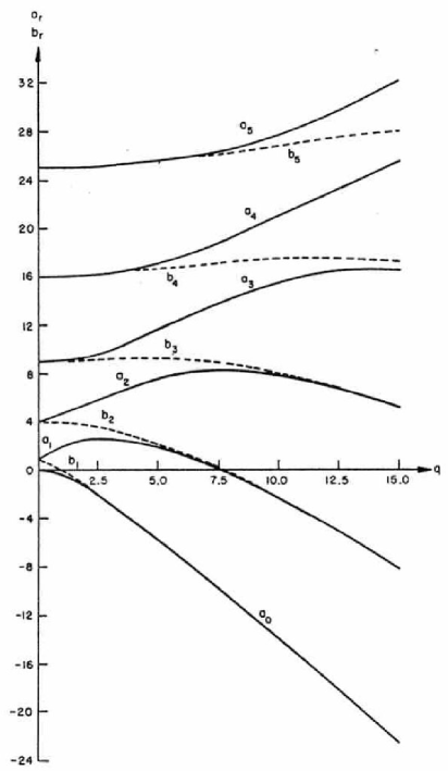
Figure 1: Phase diagram of the Mathieu equation (28). The stable regions are between the lines $a_{i}$ and $b_{i+1}$. For small $q\ll 1$ there are almost only stable regions except for thin resonance bands, while for large $q>a$ there are almost only unstable regions, except for thin stable bands. In the unstable regions the characteristic exponent $\nu$ will have a non-zero imaginary part. This figure is taken from Abramowitz .

Now we will first pose the question of stability. Let us define stability by boundedness of the generalized coordinate $x$, i.e. one could interpret it as the classical “particle” not running off to infinity exponentially fast. The answer in the classical case is given by the phase diagram of the Mathieu equation Abramowitz , see fig. 1. The first few stable bands are shown in table 1.

band # $s$	$q_{s,{\rm start}}$	$q_{s,{\rm end}}$
$1$	$0$	$0.908046$
$2$	$7.51361$	$7.57969$
$3$	$21.2986$	$21.3032$
$4$	$41.9272$	$41.9274$
$5$	$69.4284$	$69.4284$

Table 1: Stable bands in the variable $q$ of the Mathieu equation (28) for $a=0$.

As compatible with physical intuition, the stable region is roughly only given by small $q\lesssim 0.9$, except for very narrow bands in $q$. According to eq. (13) large frequencies correspond to small $q$. Thus when the potential is oscillating very rapidly, the forces practically cancel and we are left with a “free particle”. This agrees with intuition as well as the $1/\omega$ expansion. For an estimate of the amplitude of the particle position, see app. B.

2.3 Quartic potential

Turning to the $n=4$ case of the Hamiltonian (13) and applying the expansion we obtain for $V_{0}=\lambda^{5}x^{4}$ the effective Hamiltonian

$$H_{\rm eff}=\frac{P^{2}}{2m}+\frac{4\lambda^{10}}{m\omega^{2}}X^{6}+\frac{108\lambda^{10}}{m^{3}\omega^{4}}X^{4}P^{2}+\mathcal{O}(\omega^{-5})\,.$$ (17)

To our knowledge this case is not exactly solvable and hence we have nothing to add to the results of the $1/\omega$ expansion, i.e. the effective potential is confining.

3 Quantum mechanics

Following the work of Grozdanov-Raković Grozdanov:1988 and Rahav-Gilary-Fishman Rahav:2003a ; Rahav:2003b it is possible to use the method of separation of time scales also to calculate the quantum corrections to the Hamiltonian considered previously. This gives basically the effective Hamiltonian (11) (with appropriate ordering of the operators) as well as an extra quantum correction (to 4th order). The spirit of the calculation is to find a unitary transformation of the quantum Hamiltonian rendering it time independent. Again, doing so exactly is a highly non-trivial task but order by order in $1/\omega$ this can be done systematically and the resulting effective quantum Hamiltonian reads Rahav:2003a ; Rahav:2003b

$$H=\frac{p^{2}}{2m}+\frac{1}{4m\omega^{2}}[V_{0}^{\prime}]^{2}+\frac{3}{16m^{3}\omega^{4}}\left\{p,\left\{p,[V_{0}^{\prime\prime}]^{2}\right\}\right\}+\frac{\hbar^{2}}{16m^{3}\omega^{4}}\big{[}V_{0}^{(3)}\big{]}^{2}+\mathcal{O}(\omega^{-5})\,,$$ (18)

where $x$ and $p$ are now operators. Let us apply this formula to two cases in turn in the following.

3.1 Quadratic potential

In the case of $V_{0}=\lambda^{3}x^{2}$ the effective quantum Hamiltonian reads

$$H=\frac{p^{2}}{2m}+\frac{\lambda^{6}}{m\omega^{2}}x^{2}+\frac{3\lambda^{6}}{m^{3}\omega^{4}}p^{2}+\mathcal{O}(\omega^{-5})\,.$$ (19)

Note that the quantum Hamiltonian to 4th order in the $1/\omega$ expansion is exactly equal to its classical counterpart (eq. (14)) and hence also the quantum effective potential is confining. As before this is a special case and we can say a lot more than what is given by the $1/\omega$ expansion. In fact the problem can be solved also in quantum mechanics. Lewis and Riesenfeld (LR) Lewis:1968tm found a method of invariants to solve time-dependent harmonic oscillator problems. They considered the generic Hamiltonian

$$H=\frac{1}{2m}\left(p^{2}+\Omega^{2}(\tau)\,x^{2}\right)\,,$$ (20)

with $\Omega^{2}(\tau)\in\mathbb{R}$ (not positive definite) and the corresponding classical equation of motion

$$\ddot{x}+\Omega^{2}(\tau)\,x=0\,,\qquad\dot{x}=p\,.$$ (21)

Let us make a lightening review of the results of the LR-method. First we split time into three regions: a past ($\tau<\tau_{1}$) and a future ($\tau>\tau_{2}$) where the frequency of the harmonic oscillator is constant; in between we turn on the time-dependent frequency $\Omega(\tau)$, see fig. 2. If one desires, it is possible to send $-\tau_{1},\tau_{2}$ to infinity.

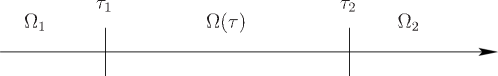
Figure 2: The frequency of the time-dependent harmonic oscillator as function of time $\tau$.

This problem admits the construction of an invariant operator called the Lewis invariant Lewis:1967

$$I=\frac{1}{2}\left[\frac{x^{2}}{\rho^{2}}+\left(\rho p-m\dot{\rho}x\right)^{2}\right]\,,$$ (22)

which obeys Heisenberg’s equation of motion while

$$m^{2}\ddot{\rho}+\Omega^{2}(\tau)\rho-\frac{1}{\rho^{3}}=0\,,$$ (23)

is the Ermakov-Pinney equation. The eigenvalues of $I$ can be shown to be time independent Lewis:1968tm , while its eigenstates are time dependent. The trick is that the eigenstates of the invariant operator $I$ can be mapped to those of the Hamiltonian and hence the transition probabilities for any given system can be calculated in terms of the eigenstates of the original Hamiltonian (20). The general solution to eq. (23) for constant $\Omega$ is Lewis:1967

$$\rho(\tau)=\pm\sqrt{|\Omega|^{-1}\left[\cosh\delta\pm\sinh\delta\sin\left(2\Omega\tau/m+\varphi\right)\right]}\ ,$$ (24)

where $\delta,\varphi\in\mathbb{R}$ are real parameters. The parameter $\delta$ encodes all information for calculating the transition probabilities from any given state at time $\tau<\tau_{1}$ to any state at time $\tau_{2}$. Unfortunately, $\delta$ is not analytically calculable, it can however be computed numerically.

For our purposes, we do not really need to calculate the occupation of particular states in detail, we merely would like to know if the quantum system is bounded in the sense that the wave function yields a bounded expectation value of the position operator, or alternatively that the average number of created particles remains bounded. The solution to the Ermakov-Pinney equation (23) can be written as follows Pinney:1950 ; Leach:2008

$$\rho(\tau)=\sqrt{au^{2}(\tau/m)+cv^{2}(\tau/m)+2bu(\tau/m)v(\tau/m)}\ ,$$ (25)

where $u(\tau/m),v(\tau/m)$ are two linearly independent solutions to eq. (21) and $ac-b^{2}=1/W^{2}$, where $W=u\dot{v}-v\dot{u}$ is the constant Wronskian of the solutions.

The argument now goes as follows, if the classical system satisfies our demand on boundedness, then the two solutions $u(\tau/m),v(\tau/m)$ are necessarily bounded and hence for any set of finite constants $\{a,b,c\}$ implied by any finite boundary condition for the quantum auxiliary function $\rho(\tau)$, its behavior will also obey the demand on boundedness. This establishes equality between boundedness of the classical and the quantum systems.

3.2 Quartic potential

In this case, $V_{0}=\lambda^{5}x^{4}$ and hence we have

$$H=\frac{p^{2}}{2m}+\frac{4\lambda^{10}}{m\omega^{2}}x^{6}+\frac{27\lambda^{10}}{m^{3}\omega^{4}}\left\{p,\left\{p,x^{4}\right\}\right\}+\frac{36\hbar^{2}\lambda^{10}}{m^{3}\omega^{4}}x^{2}+\mathcal{O}(\omega^{-5})\,.$$ (26)

This theory cannot be solved analytically and we have to rely on the assumption that the $1/\omega$ expansion is valid and equivalently the effective quantum potential is confining.

4 Field theory

4.1 Quadratic potential

Consider the Lagrangian density

$$\mathcal{L}=\frac{1}{2}(\partial_{\mu}\phi)^{2}+\frac{1}{2}m^{2}\cos(\omega t)\,\phi^{2}\,,$$ (27)

where $\phi(t,\vec{x})\in\mathbb{R}$ is a real-valued scalar field in $(d+1)$-dimensional flat spacetime, $m^{2}\in\mathbb{R}_{>0}$ and $\omega$ is an externally given fixed frequency. For convenience we choose the field to be tachyonic at time $t=0$. The equation of motion is

$$\ddot{\phi}+\left[a-2q\cos(2\tau)\right]\phi=0\,,\qquad\phi=\phi(\tau,\vec{k})\,,$$ (28)

where we have Fourier transformed the field in the spatial directions and rescaled time as $\tau\equiv\omega t/2$ while the double-dot in eq. (28) denotes the second derivative with respect to $\tau$. Eq. (28) is the Mathieu equation on canonical form Mathieu , while the parameters are related to the original Lagrangian density as follows

$$a\equiv\frac{4\vec{k}^{2}}{\omega^{2}}\,,\qquad q\equiv\frac{2m^{2}}{\omega^{2}}\,.$$ (29)

The external frequency $\omega$ sets the scale of the problem, while the parameter $q$ corresponds to the mass squared and finally the parameter $a$ corresponds to the two-norm squared of the momentum vector. $a$ is the parameter in the equation adding structure to the system due to the quantum field theory as compared to the quantum mechanics case.

There are two types of impinging instabilities threatening the system. The first is the unboundedness of the potential which we have chosen to cure by making the potential oscillate rapidly (i.e. we consider $q\ll 1$, see fig. 1). The second issue concerns resonant modes appearing upon this dynamical stabilization of the potential (i.e. for $a$ taking on integer values resonant modes appear, see fig. 1). Let us emphasize that this instability is not that of the potential being negative but merely a secondary effect due to the oscillatory behavior of the potential providing opportunity for resonances in the system at hand. The critical momentum magnitude above which all momentum modes render the potential of the theory stable is

$$k_{i}^{2}>k_{\rm critical}^{2}=m^{2}\,.$$ (30)

Above this critical momentum only the resonances reside. For a continuum of momentum modes, some modes are bound to hit the resonances, which suggests that if we want stability we should compactify space. For simplicity we will consider only toroidal compactification of the spatial dimensions. Our spacetime manifold is therefore $\mathbb{R}\times T^{d}$ and we denote the compactification radii as $R_{i}$, $i=1,\ldots,d$. Now the momenta are given in terms of a set of integers $\{n_{i}\}$ as follows

$$k_{i}=\frac{n_{i}}{R_{i}}\,,$$ (31)

and hence

$$a=\sum_{i=1}^{d}\theta_{i}n_{i}^{2}\,,\qquad\theta_{i}\equiv\frac{4}{\omega^{2}R_{i}^{2}}\,.$$ (32)

According to eq. (30) the potential becomes positive definite if we choose the compactification radii such that

$$\frac{1}{R_{i}^{2}}>m^{2}\,,\;\;\forall i=1,\ldots,d\,.$$ (33)

This ensures that there is no instability due to the potential in the theory while it does not guarantee the absence of resonances which can and do occur in general. In the remainder of this section we will study a compactification scheme such as to avoid the resonant modes entirely.

Avoiding the resonant momentum modes corresponds to choosing the parameters $\theta_{i}$ such that the quantized momentum modes hit only stable zones of the phase diagram 1; this means they should avoid hitting any integer squared $s^{2}$, $s\in\mathbb{Z}_{>0}$. The size of the unstable band can be estimated for large $s$ as Abramowitz

$$\Delta_{s}\sim\frac{q^{s}}{s^{s-1}}\,,$$ (34)

which also calls for very small $q\ll 1$. The stability condition now amounts to the following inequality

$$\left|\sum_{i=1}^{d}\theta_{i}n_{i}^{2}-s^{2}\right|>\Delta_{s}\,,$$ (35)

which we will simplify by setting all the $\theta$s equal $\theta_{i}=\theta$ (hence $R_{i}=R$) and thus

$$\left|\sum_{i=1}^{d}\frac{n_{i}^{2}}{s^{2}}-\frac{1}{\theta}\right|>\frac{e^{-sA}}{\theta\,s^{s+1}}\equiv\psi(s)\,,$$ (36)

where $A\equiv-\log q>0$.

Instead of addressing this problem directly, let us consider an easier but as we shall see, more general problem, viz. consider the stability condition

$$\left|\frac{p}{q}-\frac{1}{\theta}\right|>\psi(q)\,,$$ (37)

where $p,q\in\mathbb{Z}_{>0}$ are integers. Now the strategy is to find the best approximation $p/q$ to $1/\theta$ and try to estimate how big their difference will be as function of $q$. If it will be big enough, i.e. bigger than $\psi(q)$, then we are guaranteed absence of resonances.

Let us define $\theta^{\prime}\equiv 1/\theta$ and consider the Diophantine approximation to $\theta^{\prime}$

$$\left|\frac{p}{q}-\theta^{\prime}\right|<\frac{1}{Mq^{2}}\,,$$ (38)

where $M$ is a constant of order one depending on $\theta^{\prime}$. In general $\theta^{\prime}$ is a real number but we will consider the case where it is an irrational number, $\theta^{\prime}\in\mathbb{R}\backslash\mathbb{Q}$ and positive. It will prove convenient to utilize the continued fraction as a method for obtaining the Diophantine approximation $p/q$ to the irrational number $\theta^{\prime}$. The continued fraction is given by

$$\frac{p_{n}}{q_{n}}=a_{0}+\frac{1}{a_{1}+\frac{1}{\begin{array}[]{lll}a_{2}+\\[-9.0pt] &\ddots\\[-9.0pt] &&a_{n-1}+\frac{1}{a_{n}}\end{array}}}\,,$$ (42)

where $\{a_{i}\}$ are positive integers and $p_{n}/q_{n}$ is called the $n$-th principal convergent, while it holds that

$$\lim_{n\to\infty}\frac{p_{n}}{q_{n}}=\theta^{\prime}\,.$$ (43)

Hence if $\theta^{\prime}$ is rational a solution exists. On the other hand, if $\theta^{\prime}$ is irrational, there will only exist an arbitrarily good approximation in form of a rational number. The question is how fast it converges, viz. how good the rational number $p/q$ approximates $\theta^{\prime}$ as function of $q$. We need to invoke a few theorems due to Euler and Lagrange in order to answer that question.

Theorem 1

Lang ; Cassels For $n\geq 0$ we have

$$q_{n}p_{n-1}-p_{n}q_{n-1}=(-1)^{n}\,.$$ (44)

Corollary 1

Lang ; Cassels If $a_{1},a_{2},\ldots$ are positive integers, then $p_{n}$ and $q_{n}$ are relatively prime and $0<q_{1}<q_{2}<\cdots$ forms a strictly increasing sequence of integers.

Theorem 2

Lang ; Cassels The best approximations to $\theta^{\prime}$ are the principal convergents to $\theta^{\prime}$. In fact for $n\geq 1$, $q_{n}$ is the smallest integer $q>q_{n-1}$ such that $||q\theta^{\prime}||<||q_{n-1}\theta^{\prime}||$.

In view of the above theorem and the fact that $\{q_{n}\}$ is a strictly increasing sequence of integers, we just need to determine how good the continued fraction approximates $\theta^{\prime}$ for a given $q_{n}$.

Theorem 3

Lang ; Cassels For even $n$, the $n$-th principal convergents of $\theta^{\prime}$ form a strictly increasing sequence converging to $\theta^{\prime}$. For odd $n$, the $n$-th principal convergents of $\theta^{\prime}$ form a strictly decreasing sequence converging to $\theta^{\prime}$. Furthermore, we have

$$\frac{1}{2q_{n+1}}<\frac{1}{q_{n+1}+q_{n}}<|q_{n}\theta^{\prime}-p_{n}|<\frac{1}{q_{n+1}}\,.$$ (45)

It then follows from theorem 3 that

$$\left|\theta^{\prime}-\frac{p_{n}}{q_{n}}\right|>\frac{1}{2q_{n+1}q_{n}}\,,$$ (46)

which gives us an estimate on how bad the approximation is iff we know how much larger $q_{n+1}$ will be compared to $q_{n}$. It can be shown that

$$q_{n+1}=a_{n+1}q_{n}+q_{n-1}\,,$$ (47)

holds. Using corollary 1 we can infer that

$$q_{n+1}<(a_{n+1}+1)q_{n}\,,$$ (48)

and hence we can write eq. (46) as

$$\left|\theta^{\prime}-\frac{p_{n}}{q_{n}}\right|>\frac{1}{2(a_{n+1}+1)q_{n}^{2}}\,.$$ (49)

Comparing the two right-hand sides of eqs. (49) and (37) we arrive at the following condition

$$a_{n+1}+1<\frac{\theta}{2}q_{n}^{q_{n}-1}\exp(q_{n}A)\,,$$ (50)

which when satisfied guaranties absence of resonances.

An example which satisfies the condition (50) is the golden ratio: $1/\theta=\frac{1+\sqrt{5}}{2}$ which has the integers $a_{i}=1,i=1,2,\ldots$ and is therefore the slowest converging irrational number. Using eq. (47) it is seen the $q_{n}$s form a Fibonacci series and hence $q_{n}<q_{n+1}<2q_{n+1}$. Plugging the $a_{i}$s into eq. (50) the left-hand side is constant while the right-hand side is rapidly growing with $n$. Another example is $1/\theta=e$ having cyclic $a_{i}$s: $[a_{0},a_{1},\cdots]=[2,1,2,1,1,4,1,1,6,1,1,8,1,1,10,\cdots]$. This number also satisfies the inequality (50). Square roots of integers always have a periodic series in $\{a_{i}\}$ and hence are easy to check if they satisfy eq. (50).

The condition (50) is valid for eq. (37) which is a generalization of the problem we want to solve, namely that of eq. (36). $\sum_{i=1}^{d}n_{i}^{2}/s^{2}$ is not an arbitrary rational number $p/q$ but (for finite dimensions $d<\infty$) it is a subset of rational numbers, so the condition (50) is stronger than what we need. Thus if it is satisfied also eq. (36) is satisfied and hence there will not exist any momentum mode in the compactified field theory hitting the instability bands of the phase diagram of the Mathieu equation (no resonant modes).

4.2 Damage control

Let us consider how bad things go if one should not take our advise on the suitable values of $\theta$. We will here consider the consequences in the case that the chosen value of $\theta$ gives rise to one or more modes hitting a resonance band. We can estimate the time $t_{\Lambda}$ it takes until the norm of the unstable mode has reached the size $\Lambda$ as

$$t_{\Lambda}\sim\frac{2}{\omega|\Im(\nu)|}\log\Lambda=\frac{R\sqrt{\theta}}{|\Im(\nu)|}\log\Lambda\,.$$ (51)

In addition we need an estimate of the size of the imaginary part of the characteristic exponent $\nu$, which can be found in the literature McLachlan , valid for $q\ll a$ (an alternative method for estimating $\nu$ can be found in app. A)

$$\Im(\nu)\sim\pm\frac{\sqrt{(a_{s}-a)(a-b_{s})}}{2s}\,,$$ (52)

where $a$ is the parameter of the Mathieu equation, while $a_{s}$ ($b_{s}$) is the upper (lower) boundary of the $s$-th instability band. Let us assume the worst case scenario, i.e. the mode hitting right in the middle of the instability band giving the maximal imaginary part of $\nu$ in which case (for $q\ll 1$) $a=(a_{s}+b_{s})/2$ and hence

$$\Im(\nu_{\rm max})\sim\frac{\Delta_{s}}{4s}=\frac{q^{s}}{4s^{s}}\,,$$ (53)

where $\Delta_{s}$ is the size of the $s$-th instability band (34). This value is a rapidly decreasing function of $s$ and hence the “lifetime” in eq. (51) will be parametrically large for high enough $s$. Now that one can tolerate the large life times associated with large values of $s$, one needs to remove the thread of resonances for smaller values of $s$. There are two tools available for that; an appropriate choice of $\theta$ or a sufficiently small $R\omega$.

4.3 Quantizing the compactified field theory

We have now obtained a classical field theory which under certain conditions is stable in the sense that for each momentum mode, the equation of motion gives a – from the other modes decoupled – bounded wave function under time evolution. For a single time dependent harmonic oscillator we have seen in sec. 3.1 that the quantum state evolves in a controlled manner basically determined by the classical behavior. Let us remark that $\Omega^{2}(\tau)$ of eq. (21) is allowed to contain a non-zero constant term $a$ which is appearing in eq. (28). The time evolution of the quantum field theory state can be explicitly calculated Vergel:2009st which is basically done by acting with the Hamiltonian on a state vector living in a Schwartz space in the Schrödinger representation and finally composing an infinite product of these over all momentum modes. With respect to our stability/boundedness criteria, we are basically home free due to the fact that we are dealing with a free (i.e. non-interacting) field theory whose infinitely many harmonic oscillators are mutually uncoupled. We would however like to address the question of whether the average number of particles created remains finite, summing over all momentum modes. For that we use the solution (25) subject to the boundary conditions $\rho(0)=(\theta n^{2}-2q)^{-1/4}$ and $\dot{\rho}(0)=0$ which in turn we choose to feed with the Mathieu cosine and sine functions expanded in small $q$ (see app. B). For the characteristic exponent $\nu$ we use the approximation (106). In order to calculate the transition probability we need a quantum mechanical integration constant $\delta$ calculated for each mode $n$. The following integrated form of eq. (23) Lewis:1968tm (for $m=1$)

$$\dot{\rho}^{2}+\Omega^{2}\rho^{2}+\frac{1}{\rho^{2}}=2|\Omega|\cosh\delta\,,\qquad\Omega^{2}=\theta n^{2}-2q\cos(2\tau)\,,$$ (54)

defines $\delta$. Plugging in the above described solution $\rho$ we find

$$\cosh\delta-1= \,\frac{q^{2}}{4\theta^{2}n^{4}\left(1-\theta n^{2}\right)^{2}}\Big{\{}3+\theta n^{2}+(1-\theta n^{2})\cos(4\tau)$$ (55)

$$-2(1+\sqrt{\theta}n)\cos\left[2(1-\sqrt{\theta}n)\tau\right]-2(1-\sqrt{\theta}n)\cos\left[2(1+\sqrt{\theta}n)\tau\right]\Big{\}}+\mathcal{O}(q^{3})\,,$$

with $\tau>0$. The average number of particles $N$ Lewis:1968tm is then

$$\langle N\rangle=\sum_{n_{1},\ldots,n_{d}=1}^{\infty}\frac{1}{2}\left(\cosh\delta-1\right)\,,$$ (56)

with $n\equiv\sqrt{n_{1}^{2}+\cdots+n_{d}^{2}}$. Expanding the above expression in large $n\gg 1$ we obtain the average number of created particles

$$\langle N\rangle=\sum_{n_{1},\ldots,n_{d}=1}^{\infty}q^{2}\left(\frac{1-\cos(4\tau)}{8\theta^{3}n^{6}}+\mathcal{O}(n^{-7})\right)+\mathcal{O}(q^{3})\,,$$ (57)

from which it is seen that $\langle N\rangle$ converges for $d\leq 5$ spatial dimensions. Similarly we can calculate the total energy of the system, neglecting the mass of the created particles, as

$$E_{\rm tot}\simeq\frac{1}{R}\sum_{n_{1},\ldots,n_{d}=1}^{\infty}\frac{n}{2}\left(\cosh\delta-1\right)\,,$$ (58)

which then converges for $d\leq 4$ spatial dimensions.

4.4 Quartic potential

For the field theory

$$\mathcal{L}=\frac{1}{2}(\partial_{\mu}\phi)^{2}-\frac{\lambda}{4}\cos(\omega t)\phi^{4}\,,$$ (59)

the detailed information which was available for the quadratic potential is not readily accessible. In the following we will take a leap of faith and assume that the system thermalizes due to the fact that it is an interacting theory. The actual calculations we will perform will be related to the ABJM theory ABJM on a sphere. In the next section we consider the gravitational dual of such a theory with time-dependent couplings. In the process we will provide evidence from the bulk that the theory indeed thermalizes.

5 AdS/CFT

We will study the gravitational bulk manifestations in the regions of (in-)stabilities obtained for the boundary field theory. Our expectations are that the gravitational dual of an unstable boundary potential will result in a big crunch. For those values of parameters for which the boundary theory is eventually stable, we expect that a black hole (BH) horizon will form. We will consider the setup of 11-dimensional supergravity in AdS${}_{4}\times(S^{7}/\mathbb{Z}_{k})$ as a ground on which to identify the appropriate bulk field configurations, corresponding to the different types of boundary potentials we study. $\mathcal{N}=8$ supergravity in four dimensions describes the massless sector of the compactified 11-dimensional supergravity on $S^{7}$. It is possible to introduce a consistent truncation involving only gravity as well as a single scalar field $\phi$ Duff:1999gh . We thus consider the following effective action

$$S=\int d^{4}x\,\sqrt{-g}\left(\frac{R}{2}-\frac{1}{2}\partial_{\mu}\phi\partial^{\mu}\phi-V(\phi)\right)\,,$$ (60)

with $V(\phi)=-2-\cosh(\sqrt{2}\phi)\approx-3-\phi^{2}+O(\phi^{4})$. As pointed out in Craps:2009qc ; Bernamonti:2009dp , the same consistent truncation can be used for the more general compactification of 11-dimensional supergravity on the quotient space $S^{7}/\mathbb{Z}_{k}$. The scalar field $\phi$ has a mass squared $m^{2}=-2$, which is above the Breitenlohner-Freedman bound BF $m_{\rm BF}^{2}=-9/4$. The AdS metric in global coordinates can be written as

$$ds^{2}=-(1+r^{2})\,dt^{2}+\frac{dr^{2}}{1+r^{2}}+r^{2}\,d\Omega_{2}^{2}=-\frac{dt^{2}}{\cos^{2}x}+\frac{dx^{2}}{\cos^{2}x}+\tan^{2}x\,d\Omega_{2}^{2}\,,$$ (61)

where $r=\tan x$. The scalar field goes to zero asymptotically as

$$\phi(r)\approx\frac{\alpha}{r}+\frac{\beta}{r^{2}}\,.$$ (62)

According to the AdS/CFT correspondence, M-theory in global ${\rm AdS}_{4}\times(S^{7}/\mathbb{Z}_{k})$ is dual to ABJM theory ABJM on $S^{2}\times\mathbb{R}$, i.e. a ${\rm U}(N)\times{\rm U}(N)$ superconformal Chern-Simons (CS) theory with matter and CS levels $+k$ and $-k$. It contains four $\mathcal{N}=2$ chiral superfields $Y_{s}$ transforming in the $(N,\bar{N})$ representation of the gauge group. Due to the conformal coupling, the four scalars $Y_{s}$ acquire masses proportional to $1/R_{S^{2}}$ which we set to unity. The field $\phi$ of the consistent truncation in eq. (60) corresponds to the following scalar mass operator in ABJM theory

$$\mathcal{O}=\frac{1}{N}{\rm Tr}\left(Y_{1}Y_{1}^{\dagger}+Y_{2}Y_{2}^{\dagger}-Y_{3}Y_{3}^{\dagger}-Y_{4}Y_{4}^{\dagger}\right)\,.$$ (63)

Multitrace deformations Witten:2001ua ; BSS of the form $S=S_{0}-N^{2}W(\mathcal{O})$, correspond to the following boundary condition

$$\beta=W^{\prime}(\alpha)\,.$$ (64)

This is possible due to the fact that the mass of the scalar field lies in the interval

$$-\frac{9}{4}<m^{2}<-\frac{5}{4}\,,$$ (65)

and hence both scalar-wave fall offs of eq. (62) are normalizable.

By appropriately choosing $W(\mathcal{O})$, it is possible to construct unbounded potentials in the boundary theory for which $Y_{s}=0$ is a metastable vacuum; for instance by choosing $W=H_{3}\mathcal{O}^{3}/3$ with an arbitrary sign for $H_{3}$, or alternatively $W=H_{2}\mathcal{O}^{2}/2$ with $H_{2}<0$. The first case corresponds to AdS-invariant boundary conditions Hertog:2004dr . We first study the case of a time-independent unstable potential and identify the bulk signature of that and then we introduce time dependence HH1 .

5.1 Instantons and crunches

Let us first consider the case of a time-independent multitrace operator. When the multitrace operator renders the boundary theory metastable, this metastability manifests itself in the bulk as a Coleman-de Luccia instanton CdL when the multitrace operator is marginal and by some other type of bubble when it is a relevant operator Barbon:2010gn ; Barbon:2011ta . In the AdS₄ setting we are considering, instantons were studied in detail in HH1 ; HH2 . The following spherically symmetric Ansatz for the metric is used

$$ds^{2}=\left(\frac{d\rho^{2}}{b^{2}(\rho)}+\rho^{2}d\Omega_{3}^{2}\right)\,.$$ (66)

The Euclidean action reads

$$S=\int d^{4}x\,\sqrt{g}\left(-\frac{R}{2}+\frac{1}{2}\partial_{\mu}\phi\partial^{\mu}\phi+V(\phi)\right)-\int_{\partial}d^{3}x\sqrt{h_{c}}K+\,S_{\rm ct}\,+\,S_{\partial}\,,$$ (67)

where $h_{c}$ is the induced metric on the cutoff surface, $K$ is the trace of the extrinsic curvature of the boundary (giving the Gibbons-Hawking term), $S_{\rm ct}$ and $S_{\partial}$ contain counter terms and the boundary terms, respectively. In the AdS₄ setup with $m^{2}=-2$ which we study, $S_{\rm ct}$ and $S_{\partial}$ take the forms Balasubramanian:1999re ; Papadimitriou:2007sj

$$S_{\rm ct}=\int_{\partial}d^{3}x\,\sqrt{h_{c}}\left(2+\frac{R(h_{c})}{2}+\frac{1}{2}\Delta_{-}\phi^{2}\right)\,,\qquad S_{\partial}=\int_{\partial}d^{3}x\,\sqrt{h}\left(W(\alpha)-\alpha W^{\prime}(\alpha)+\alpha\beta\right)\,,$$

where $\Delta_{-}=1$, $h$ is the induced metric on the boundary and $R(h_{c})$ is the Ricci scalar of the induced metric on the cutoff surface.

Using the $\rho$ coordinate, the equation of motion for the instanton is

$$b^{2}=\frac{2\rho^{2}V(\phi)-6}{\rho^{2}(\phi^{\prime})^{2}-6}\,,\qquad b^{2}\phi^{\prime\prime}+\left(bb^{\prime}+\frac{3b^{2}}{\rho}\right)\phi^{\prime}-V^{\prime}(\phi)=0\,.$$ (68)

For numerical convenience we make a change of variables as follows; instead of $\rho$ we will use $x=\tan^{-1}\rho$; and instead of $b$, $A=b^{2}/(\rho^{2}+1)$. The equation of motion for the instanton then reads

$$\phi^{\prime\prime}+\left(\frac{2+\cos^{2}x}{\sin x\cos x}+\frac{A^{\prime}}{2A}\right)\phi^{\prime}-\frac{V^{\prime}(\phi)}{A\,\cos^{2}x}=0\,,\qquad A=\frac{2V(\phi)\sin^{2}x-6\cos^{2}x}{\sin^{2}x\cos^{2}x(\phi^{\prime})^{2}-6}\,.$$ (69)

which is sometimes conveniently written as

$$\phi^{\prime\prime}=\frac{1}{A}\left(\frac{V^{\prime}}{\cos^{2}x}+\frac{\sin 2x}{6}(V+3)\phi^{\prime}\right)-\frac{2+\cos^{2}x}{\sin x\cos x}\phi^{\prime}+\frac{\sin 2x}{12}\left(2+\sin^{2}x\right)(\phi^{\prime})^{3}\,.$$ (70)

Fig. 3 shows an example of an instanton solution. The family of solutions is parametrized by the value $\phi_{0}\equiv\phi(0)$, i.e. the value of the scalar field at the origin. Each of these solutions corresponds to a particular value of $(\alpha,\beta)$ of eq. (62) at infinity; see fig. 4. The limit $\phi_{0}\rightarrow 0$ corresponds to $H_{3}\rightarrow\pm\infty$ for tripletrace deformations, while for doubletrace deformations $H_{2}\rightarrow-1$.

 

(a) $\phi(x)$

(b) $A(x)$

Figure 3: Instanton solution with $\phi_{0}=0.1$.

Figure 4: Left panel: $\alpha$ (solid line) and $\beta$ (dashed line) for the instanton as function of $\phi_{0}$. Right panel: $H_{2}=\beta/\alpha$ as function of $\phi_{0}$.

The decay rate can be computed in terms of the Euclidean action of the instanton, using the Coleman-de Luccia CdL method. The relevant quantity determining the tunneling rate is $e^{-(S-S_{\rm AdS})/\hbar}$, with $S$ being the instanton action and $S_{\rm AdS}$ the void AdS action. In the tripletrace case, it was checked in HH1 that $S-S_{\rm AdS}$ is a finite quantity and hence the tunneling occurs in a finite time. We checked that this is also the case for the doubletrace deformation with negative $H_{2}$.

After the tunneling occurs, the initial condition is obtained by restricting the instanton solution to the equator. In the case of AdS-invariant boundary conditions with a tripletrace deformation, time evolution can be obtained directly via analytical continuation of the instanton. Inside the lightcone the metric has the form of a Friedmann-Robertson-Walker solution

$$ds^{2}=-dt^{2}+a^{2}(t)\left(dr^{2}+\sinh^{2}r\,d\Omega_{2}^{2}\right)\,,$$ (71)

with equations of motion

$$\dot{a}^{2}=1+\frac{a^{2}}{3}\left(\frac{\dot{\phi}^{2}}{2}+V(\phi)\right)\,,\qquad\ddot{\phi}+3\frac{\dot{a}}{a}\dot{\phi}+V^{\prime}(\phi)=0\,,$$ (72)

describing a universe which is initially expanding but then eventually contracting; thus developing a big crunch singularity within a finite time CdL .

5.2 Black holes

We recall that the Einstein-scalar theory (60) has also other time-independent solutions than empty AdS. For all values of $H_{2}$ and $H_{3}$ the AdS-Schwarzschild BH is a solution with the metric

$$ds^{2}=-\frac{Ae^{-2\delta}}{\cos^{2}x}\,dt^{2}+\frac{dx^{2}}{A\,\cos^{2}x}+\tan^{2}x\,d\Omega^{2}_{2}\,,\qquad A=1-\frac{M_{\rm BH}}{4\pi}\frac{\cos^{2}x}{\tan x}\,,$$ (73)

with $\delta=0$. The mass and the temperature as a function of the horizon $x_{h}$ are

$$M_{\rm BH}=4\pi\frac{\tan x_{h}}{\cos^{2}x_{h}}\,,\qquad T_{\rm BH}=\frac{1}{4\pi}\left(3\tan x_{h}+\frac{1}{\tan x_{h}}\right)\,,$$ (74)

and the specific heat is negative for $x_{h}<\pi/6$.

More general BH solutions with scalar hair have been studied in Hertog:2004dr ; among the time-independent solutions, there are also solitons without horizons, see e.g. HH1 ; Hertog:2004ns . The time-independent equations of motion read

$$\frac{1}{\tan^{2}x}\left(\tan^{2}xAe^{-\delta}\Psi\right)^{\prime}-\frac{d\,V}{d\,\phi}e^{-\delta}\frac{1}{\cos^{2}x}=0\,,\qquad\delta^{\prime}=-\frac{\sin x\cos x}{2}\,\Psi^{2}\,,$$ (75)

$$A^{\prime}=\frac{1+2\sin^{2}x}{\sin x\cos x}(1-A)-\frac{\sin x\cos x}{2}A\Psi^{2}-(V(\phi)+3)\tan x\,,$$ (76)

where $\Psi\equiv d\phi/dx$. At the horizon $x_{h}$ (defined by $A(x_{h})=0$) the following boundary condition should be imposed

$$\Psi=\frac{\tan x}{1-V(\phi)\tan^{2}x}\frac{1}{\cos^{2}x}\frac{d\,V}{d\,\phi}\,.$$ (77)

All these time-independent solutions Hertog:2004dr ; HH1 ; Hertog:2004ns have a negative ratio $H_{2}=\beta/\alpha<0$. The only time-independent solution compatible with $H_{2}\geq 0$ is the Schwarzschild BH, which is a solution for arbitrary $H_{2}$.

We will next proceed to uncovering the duals of time-dependent boundary theories; the BH will be a good candidate to screen the big-crunch singularity for those cases where we will find that dynamical stabilization occurs.

5.3 Time-dependent equations of motion

We now turn to matching the gravitational solutions to time-dependent boundary conditions. This requires in turn, that the bulk solutions be time dependent. To this end we consider a spherically symmetric setup, with the metric

$$ds^{2}=-\frac{e^{-2\delta(x,t)}A(x,t)}{\cos^{2}x}dt^{2}+\frac{dx^{2}}{A(x,t)\,\cos^{2}x}+\tan^{2}x\,d\Omega^{2}_{2}\,.$$ (78)

as well as a scalar field $\phi(x,t)$. The cross term $dx\,dt$ is absent from the metric due to the choice of gauge. There is still some freedom in shifting the variable $\delta$ by a function of time; this corresponds a time re-parametrization. In the following we will set $\delta=0$ at $x=\pi/2$, such that $t$ is the global time coordinate in asymptotic AdS space.

Let us introduce the auxiliary variables $\Psi=\phi^{\prime}$ and $\Pi=A^{-1}e^{\delta}\dot{\phi}\,$ (where $\,{}^{\prime}\,$ denotes derivative with respect $x$ and $\,\dot{}\,$ with respect to $t$) for which the equations of motion read

$$(Ae^{-\delta}\Pi)^{\prime}=\dot{\Psi}\,,\qquad\frac{1}{\tan^{2}x}\left(\tan^{2}xAe^{-\delta}\Psi\right)^{\prime}-\frac{d\,V}{d\,\phi}e^{-\delta}\frac{1}{\cos^{2}x}=\dot{\Pi}\,,$$ (79)

$$A^{\prime}=\frac{1+2\sin^{2}x}{\sin x\cos x}(1-A)-\frac{\sin x\cos x}{2}A(\Psi^{2}+\Pi^{2})-(V(\phi)+3)\tan x\,,$$ (80)

$$\delta^{\prime}=-\frac{\sin x\cos x}{2}(\Pi^{2}+\Psi^{2})\,,\qquad\phi^{\prime}=\Psi\,,$$ (81)

$$\dot{\phi}=\Pi Ae^{-\delta}\,,\qquad\dot{A}+(\sin x\cos x)A^{2}e^{-\delta}\Psi\Pi=0\,.$$ (82)

The last equation of (82) is a consequence of the other ones.

In order for the solution to be smooth, we must require that $\Psi|_{x=0}=\Pi^{\prime}|_{x=0}=A^{\prime}|_{x=0}=\Pi|_{x\to\pi/2}=A^{\prime}|_{x\to\pi/2}=0$ and $A|_{x=0}=A|_{x\to\pi/2}=1$; both $\Pi|_{x=0}$ and $\Psi|_{x\to\pi/2}$ are non-vanishing functions of time. The quantities $(\alpha,\beta)$ are directly related to the values of $\Psi$ and $\Psi^{\prime}$ at the boundary

$$\Psi(\pi/2)=-\alpha\,,\qquad\Psi^{\prime}(\pi/2)=2\beta\,.$$ (83)

Near the boundary, $\phi$ is going to zero linearly in $(\pi/2-x)$, while $\Psi$ is finite. In the following we will specialize our treatment to time-dependent boundary conditions of the form

$$W=\frac{H(t)}{2}\mathcal{O}^{2}\,,\qquad H(t)=H_{2}(t)=\frac{\beta(t)}{\alpha(t)}\,,$$ (84)

corresponding to doubletrace operators. The boundary conditions at $x\rightarrow\pi/2$ are

$$\Psi^{\prime}=-2H\Psi\,,\qquad\Pi^{\prime\prime}=-2\dot{H}\Psi-2H\Pi^{\prime}\,.$$ (85)

5.4 Observables

In this section we will define some useful observables describing geometric features of the numerical solutions. The first observable we address is the scalar curvature, which by means of the equations of motion, is

$$R=4V(\phi)+A(\Psi^{2}-\Pi^{2})\cos^{2}x\,.$$ (86)

The second observable we need is the total energy for which it proves convenient to express the metric component $g_{rr}$ in terms of the function $A(x)$. Setting $A(\pi/2)=1$ and $A^{\prime}(\pi/2)=0$ we get

$$g_{rr}=\frac{1}{r^{2}}-\left(1+\frac{A^{\prime\prime}(\pi/2)}{2}\right)\frac{1}{r^{4}}+\frac{A^{(3)}(\pi/2)}{6}\frac{1}{r^{5}}+\ldots$$ (87)

Expanding eq. (80) in series around $x=\pi/2$, it follows that $A^{\prime\prime}(\pi/2)=\Psi^{2}(\pi/2)=\alpha^{2}$. Using an expression for the total energy given in Hertog:2004ns , we obtain

$$M=4\pi\left(\frac{A^{(3)}(\pi/2)}{6}+\alpha\beta+\int_{0}^{\alpha}\beta(\tilde{\alpha})d\tilde{\alpha}\right)=4\pi\left(\frac{A^{(3)}(\pi/2)}{6}+\frac{3}{2}H\alpha^{2}\right)\,.$$ (88)

This quantity is in general not constant, because the time-dependent multitrace operator acts as an external source of energy for the conformal field theory described by the AdS₄ geometry.

A trapped two-surface $\mathcal{S}$ (see e.g. book ) is defined as a closed surface with the property that the expansion scalars

$$\theta_{l}=(g^{ab}+l^{a}n^{b}+l^{b}n^{a})\nabla_{a}l_{b}\,,\qquad\theta_{n}=(g^{ab}+l^{a}n^{b}+l^{b}n^{a})\nabla_{a}n_{b}\,.$$ (89)

in each of the two forward-in-time null directions $l_{a},n_{b}$ (normal to $\mathcal{S}$) are both negative. We use the cross normalization $l_{a}n^{a}=-1$. Then, considering a foliation by spacelike three-surfaces $\Sigma_{t}$, a point $q\in\Sigma_{t}$ is said to be trapped if it lies on a trapped two-surface $\mathcal{S}$ in $\Sigma_{t}$. The apparent horizon in $\Sigma_{t}$ is thus constructed as the boundary of the union of all the trapped points. Let us consider the following null direction of ingoing and outgoing wave fronts in the $(t,x)$ direction

$$l_{a}=\frac{1}{\sqrt{2A}e^{\delta}\cos x}\{-A,-e^{\delta},0,0\}\,,\qquad n_{a}=\frac{1}{\sqrt{2A}e^{\delta}\cos x}\{-A,e^{\delta},0,0\}\,.$$ (90)

An explicit calculation gives

$$\theta_{l,n} =\mp\frac{\sqrt{2A}}{\sin x}\,.$$ (91)

This shows that no apparent horizon forms as long as $A$ remains positive.

The metric (78) is an example of polar coordinates, which are in general defined by the condition $\mathcal{K}^{\theta}_{\theta}=\mathcal{K}^{\phi}_{\phi}=0$, where $\mathcal{K}$ is the extrinsic curvature tensor. It is a general feature of polar coordinates that they can not be used to parametrize events happening inside apparent horizons (see e.g. lectures ; book for a discussion); instead they become singular when an apparent horizon forms. Apparent horizons are then detected by the condition that the metric (78) is singular lectures ; book , which is therefore given by a vanishing $A$. An alternative foliation and metric Ansatz should be used in order to penetrate the apparent horizons.

5.5 Numerical results

In this section we present numerical solutions of eqs. (79-82) obtained for different time-dependent boundary conditions, specified by the function $H(t)$ in eq. (84). As initial condition we use the instanton obtained by eqs. (69,70) restricted to the equator. We imagine that $H(t)$ is constant for $t<0$ and that the system is in a metastable vacuum. We then assume that a tunneling occurs at $t=0$ from where we introduce time dependence to the doubletrace deformations. As a parametrization of the instanton solutions, we fix $\phi_{0}$, corresponding to the value of the scalar field at the origin of the instanton. The relation between $\phi_{0}$ and the initial value of $H(t)=H_{2}$ is shown in fig. 4.

We first consider the case of constant $H(t)=h_{0}<0$ for which the solution corresponds to big crunch geometries. A curvature singularity (which extends to the boundary) develops in a finite time. The energy can be computed via eq. (88) which we have checked is diverging at the time when the crunch singularity forms. A plot of the time it takes for each instanton to evolve into a crunch as function of $\phi_{0}$ is shown in fig. 5. This quantity increases with the steepness of the potential. The reason for this is that the larger the value of $\phi_{0}$ is, the larger is the energy which causes the crunch. Note on the other hand the smaller the value of $\phi_{0}$ is, the faster is the decay of the vacuum. This behavior can be seen in the right-hand part of fig. 4.

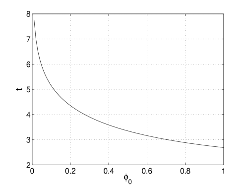
Figure 5: The time it takes for an instanton to evolve into a big crunch singularity for constant and negative $H(t)=h_{0}<0$ as function of $\phi_{0}$.

Let us next consider a boundary condition of the type

$$H(t)=h_{0}\left(2e^{-t^{2}}-1\right)\,,\qquad h_{0}<0\,,$$ (92)

which from the boundary point of view corresponds to a negative and unbounded potential at the initial time, but is then lifted in a finite time $\approx 2$ to a positive definite one. A solution within this class is shown in fig. 6. For a massless particle in AdS space, it takes the time $\pi$ to reach the boundary and come back to the origin, corresponding to a frequency $\omega_{0}=2$. Indeed in the plots both the fields and the curvature oscillate with a frequency of roughly $2$.

   

(a) $\phi(x,t)$

(b) $A(x,t)$

(c) $\delta(x,t)$

(d) scalar curvature $R(x,t)$

Figure 6: A solution with boundary condition (92) and $\phi_{0}=0.1$. The initial negative unbounded potential is lifted to a constant positive definite one in a finite time $t\approx 2$ much before the time when the crunch singularity would have formed if the unbounded potential were kept constant (see figure 5). The resulting configuration in this case is just a scalar wave reflected by the AdS boundary conditions.

At late times we expect a BH to form due to the weak turbulent instability discussed in Bizon ; Dias ; deOliveira:2012ac . However, in the regime of small $\phi_{0}$ the horizon forms only after a very long time and after the scalar field has bounced off the AdS boundary many times. The time of BH formation as function of $\phi_{0}$ is shown in fig. 7. For computational constraints we computed the solutions only till time $t_{\rm max}=40$. In the cases where a horizon has formed during the finite calculation time, we have checked that the final configuration is, to a good approximation, a Schwarzschild BH outside the horizon.

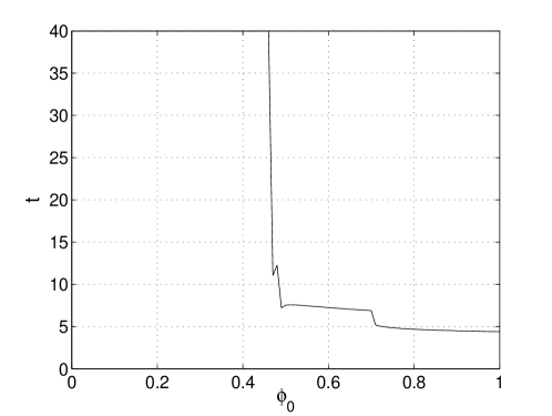
Figure 7: The time after which a BH is formed as function of $\phi_{0}$, for the boundary condition (92). The simulation is run until $t_{\rm max}=40$. For $\phi_{0}\leq 0.46$ we notice a very sharp transition: no horizon forms before $t_{\rm max}$; for $\phi_{0}=0.46$, it is found that a BH horizon forms at $t\approx 882$.

We are now ready to study the boundary conditions related to dynamical stabilization. These alternate between a negative, unbounded potential and a positive one

$$H(t)=h_{0}\cos(\omega t)\,,\qquad h_{0}<0\,.$$ (93)

For sufficiently small $\omega$ a crunch will occur, otherwise given a general point in the parameter space $(\phi_{0},\omega)$ a crunch may or may not form at some point in the future. A plot of the parameters for which a big crunch singularity forms (before time $t_{\rm max}=40$) is shown in fig. 8.

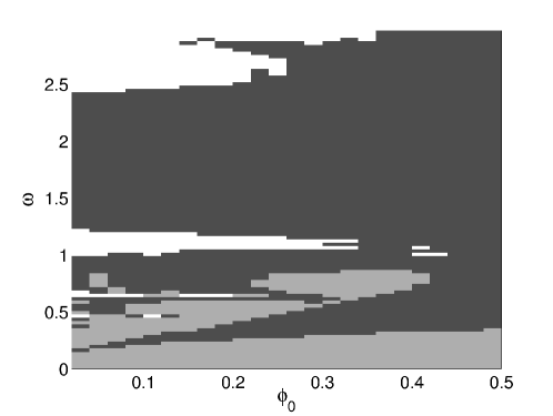
Figure 8: Shown in light gray, points in parameter space giving rise to a crunch before $t_{\rm max}=40$, for the boundary condition in eq. (93). The points for which a BH is formed before $t_{\rm max}$ are shown in dark gray. Points in parameter space for which neither a crunch nor a BH is formed before $t_{\rm max}$ are shown in white.

The transition between the crunch and the BH regime should correspond to a BH with infinite mass. This regime however is challenging to study numerically as it is sensitive to the UV cutoff $x_{\rm max}$ which in turn requires increasingly small finite difference steps.

An example of a solution where a horizon forms is shown in fig. 9. As explained in section 5.4, a horizon can be detected by virtue of a vanishing $A$. The scalar curvature $R$ becomes quite large inside the horizon. The time evolution after the time where $A$ vanishes cannot be trusted, because the metric becomes singular and hence cannot be used to parametrize events inside the apparent horizon.

 

(a) $\phi(x,t)$

(b) $A(x,t)$

(c) $\delta(x,t)$

(d) scalar curvature $R(x,t)$

Figure 9: A solution where a BH forms for $\phi_{0}=0.1$ and $\omega=0.9$, corresponding to a dark gray point in fig. 8. Dynamical stabilization is at work: the big crunch singularity does not reach the boundary in a finite time as it is screened by an apparent horizon, which is where $A=0$. The absolute value of the scalar curvature (d) becomes large (signaling the formation of a singularity), but it happens inside the horizon.

An example of a parameter point where no horizon forms before time $t_{\rm max}=40$ is shown in fig. 10. Here the scalar curvature remains rather small everywhere. The curvature and the scalar field at $x=0$ are shown as function of time in fig. 11.

   

(a) $\phi(x,t)$

(b) $A(x,t)$

(c) $\delta(x,t)$

(d) scalar curvature $R(x,t)$

Figure 10: A solution where no BH forms before $t_{\rm max}=40$ for $\phi_{0}=0.1$ and $\omega=3.0$, corresponding to a white point in fig. 8. Dynamical stabilization is also at work here, even if no BH horizon has formed before $t_{\rm max}$. The solution corresponds to a scalar wave being reflected many times by the time-dependent boundary condition, without a dramatic increase of the total energy. The field configuration is similar to that of fig. 6, even though the stabilization in the latter case is not dynamical.

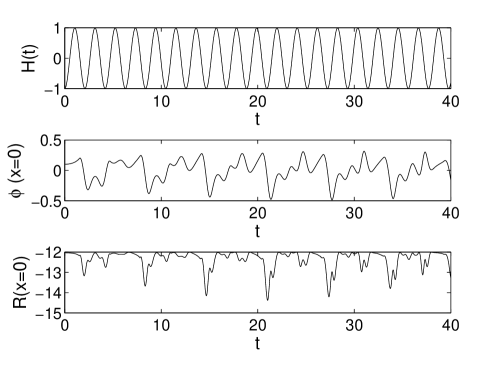
Figure 11: The value of $\phi$ and the scalar curvature $R$ at $x=0$ are shown as functions of time for $\omega=3$ and $\phi_{0}=0.1$. For comparison also the driving potential $H(t)$ is shown.

For sufficiently large frequencies, we have checked that in the case that no horizon has formed before $t_{\max}$, the maximum of the energy and the maximum of $|R|$ remained small (see figure 12). When a horizon forms, the scalar curvature $|R|$ tends to become large; however this all happens inside of the horizon. The energy of the resulting BH does not diverge, on the contrary it tends to become smaller for increasingly larger frequencies. In fig. 13 is shown the time of horizon formation as function of $\omega$ for $\phi_{0}=0.1$.

There are sharp transitions in the time of BH formation as a function of $\omega$ (see fig. 13). For frequencies $\omega$ around even integer values, a BH forms rather quickly, whereas for frequencies $\omega$ near odd integer values, we have observed no BH formation before stopping the numerical code at $t=800$. A field propagating with the speed of light takes the time $\pi$ to reach the boundary and return from $x=0$; this corresponds exactly to the frequency $\omega_{0}=2$. Perhaps this provides some qualitative explanation for how come BHs form more easily subject to even frequencies.

Figure 12: Left panel: Maximum of the energy as function of $\omega$ for $\phi_{0}=0.1$. Right panel: Maximum and minimum of the scalar curvature $R$ as functions of $\omega$. The $*$s correspond to the minimum of $A$ in some units, showing the correlation between the latter quantities and the formation of a horizon.

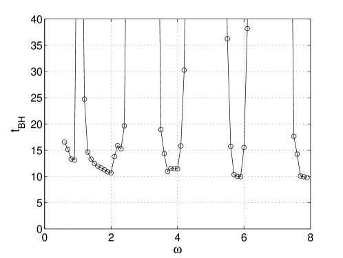
Figure 13: The time of horizon formation as function of $\omega$ for $\phi_{0}=0.1$. In some intervals of frequency centered around $\omega$ taking on even integer values, a BH horizon formation occurs rather quickly. On the other hand, we have observed no BH formation for odd integer values, $\omega=3,5,7$, in calculations running up to the time $t=800$. Horizon formation at $t=220$ is observed for $\omega=1$, while no BH formation is observed up to $t=800$ for $\omega=1.17$.

Two options are possible upon horizon formation. Either the solution tends to a Schwarzschild BH at late times, as it is the only time-independent solution compatible with our boundary conditions or alternatively the BH will be time-dependent and its size and mass will increase indefinitely – we are effectively pumping energy into the system. Unfortunately our choice of metric Ansatz (78) is not permitting us to study this issue, because it becomes singular as soon as the horizon has formed.

In the case of a massless scalar in flat 4-dimensional spacetime, Choptuik found for an arbitrary family of solutions parametrized by $p$, that both the critical horizon radius and the BH mass scale as $(p-p_{*})^{\gamma}$, where $\gamma\approx 0.37$ and $p_{*}$ is the critical value for BH formation Choptuik . An identical scaling was found for AdS₄ with a massless scalar in Husain:2002nk ; Bizon . For a massive field in flat space (e.g. Brady:1997fj ), depending on the class of solutions considered, it is also possible that BH formation begins at finite mass and radius (type I transition), instead of beginning at infinitesimal mass (type II transition). In the case of a type II transition, the same critical exponent $\gamma$ was found as in the massless case. The exponent $\gamma$ is not universal for all kinds of matter; for example, in the case of type II transitions in Einstein-Yang-Mills equations Choptuik:1996yg , $\gamma\approx 0.2$, (for a review of critical gravitational collapse with various kinds of matter, see Gundlach:2007gc ).

In AdS₄ with a tachyonic scalar in the mass range (65), it is in principle possible to study both the critical behavior as function of the initial field profile, as well as function of the boundary condition at $x\rightarrow\pi/2$. The boundary condition (92) gives rise to a type II transition, which we have observed due to the formation of arbitrarily small BH horizons with critical value $\phi_{0c}\approx 0.468$. On the other hand, for the boundary conditions (93) and fixed $\phi_{0}=0.1$, there are several type I transitions as a function of $\omega$: for example, BH formation begins at radius $\approx 0.5$ and $t=64$ for $\omega=1.175>\omega_{c}$, while no BH horizon has formed before $t=800$ for $\omega=1.17<\omega_{c}$. We leave a more accurate study of these transitions and a determination of the critical exponents in case of a type II transition for future work.

5.6 Numerical scheme

We solve the time-dependent PDEs using the leapfrog method with a five-point – 4th order difference stencil for the spatial derivatives, a grid of $2500$ points and Courant number $0.5$. Explicit dissipative terms are added. The instanton solution (taken as the initial condition) is obtained by solving eqs. (69,70) using 5th order Runge-Kutta. In order to initialize the leapfrog algorithm, we need to provide the first and second order time derivatives of the initial instanton profile function. We set all the first order time derivatives to zero, except

$$\dot{\Pi}=-\frac{\Psi e^{-\delta}}{\tan x}\,.$$ (94)

The second derivatives read

$$\ddot{\Psi}=-e^{-2\delta}\left(\frac{V^{\prime}(\phi)}{\cos x\sin x}+\left(V(\phi)-\frac{4}{\tan^{2}x}\right)\Psi\right)\,,\qquad\ddot{\phi}=-\frac{\Psi Ae^{-2\delta}}{\tan x}\,,$$

$$\ddot{A}=A^{2}e^{-2\delta}\Psi^{2}\cos^{2}x\,,$$ (95)

and $\ddot{\Pi}=0$. No simple expression for $\ddot{\delta}$ is available and hence $\delta$ is recalculated using eq. (81). For practical reasons we introduce an IR and a UV cutoff $x_{\rm min}=0.001$ and $x_{\rm max}=1.565$ (if we use values of $x_{\rm max}$ closer to $\pi/2$, the corresponding boundary conditions make the numerics unstable). In order to update $\phi$ at the boundary $x_{\rm max}$ and $A$ at the origin $x_{\rm min}$ we use eqs. (82). Subsequently eqs. (80,81) are solved using a 5th order Runge-Kutta method. The boundary value $\delta(x_{\rm max})$ is fixed to be zero. The eqs. (82) are then used to estimate the numerical accuracy.

6 Discussion

In this note we have discussed the issue of dynamical stability in various examples of theories with time-dependent potentials which are periodically unbounded from below. Considering an oscillating quadratic potential in the case of classical and quantum mechanics as well as in field theory, the stability regions are encoded by the phase diagram of the Mathieu equation. The zero mode is stabilized when the frequency is high enough. In addition we found a compactification scheme relying on number theory such as to avoid resonances in all momentum modes of the field theory. The effective Hamiltonian for periodically driven systems Rahav:2003a ; Rahav:2003b suggests that a similar dynamical stabilization occurs also for interacting theories. We have found numerical evidence for this in a theory with an AdS/CFT dual; for sufficiently large $\omega$ the big-crunch singularity is screened by a black hole horizon, preventing the crunch singularity to reach the boundary in a finite time. We have observed sharp transitions in the black hole formation time as function of the frequency $\omega$. For frequencies near even integer values, horizons form rather quickly while for those near odd integer values, we have observed black hole formation at very late times or not at all, due to finite simulation time.

In fact we would be curious to see if such a potential could be a holographic description of a universe oscillating between bangs and crunches or healed bangs and healed crunches. An analytic study of such system was carried out in Nappi:1992kv ; Kounnas:1992wc ; Liu:2002ft ; Elitzur:2002rt ; Gasperini:2002bn and references therein, but there the system had an infinite amount of boundaries and in the presence of closed time-like curves. One could wish that all this could be encapsulated on a single boundary without redundant features. This could have been a system for which the time-dependent couplings on the boundary are appropriate. Unfortunately, for this, the numerical analysis is not a substitute for an exact solution. It is worthwhile to study such systems non-perturbatively even if there is a lack of a strong phenomenological motivation at this stage.

Let us comment on possible topics of future directions:

• For the free field theory part one could consider different compactifications of the spatial dimensions to see if this gives rise to additional structure.

• It would be challenging to follow the black hole evolution after the horizon has formed; for this it might be necessary to use a different (non-polar) metric Ansatz and also introduce a singularity excision, e.g. as in Pretorius ; Chesler:2008hg ; Heller:2012je .

• We did not address here the precise nature of the transition between the big crunch and black hole of infinite mass; for example, it would be interesting to determine the dependence of the black hole mass near the critical frequency $\omega_{c}$ separating the black hole regime from the crunch.

• A more detailed study of the transition type (I or II) at the threshold of black hole formation, both as a function of initial field profile $\phi_{0}$ and of the time-dependent boundary condition $\omega$, would be worthwhile to investigate; in particular calculating the critical exponents for the type II transition.

Appendix A Estimating the characteristic exponent

The characteristic exponent $\nu$ can be estimated numerically by calculating the solution $y(\tau)$ to eq. (28) subject to the boundary conditions $y(0)=1$, $\dot{y}(0)=0$, and then evaluated at $\tau=\pi$ Abramowitz

$$\cos(\nu\pi)=y(\pi)\ ,$$ (96)

where $\nu$ is implicitly a function of $a,q$.

Appendix B Estimating the amplitude

From the interpretation that the generalized coordinate $x$ describes a particle, a natural question would be how far the particle goes. Let us first consider the simple example of a particle at rest and situated at position $x(0)=1$ at time $\tau=0$. Using an expansion valid for small $q\ll 1$ and $\nu$ real but not an integer, the solution reads Abramowitz

$$C(\tau)= \;\frac{\cos[\nu\tau]-\frac{q\cos\left[(\nu+2)\tau\right]}{4(\nu+1)}+\frac{q\cos\left[(\nu-2)\tau\right]}{4(\nu-1)}+\frac{q^{2}\cos\left[(\nu+4)\tau\right]}{32(\nu+1)(\nu+2)}+\frac{q^{2}\cos\left[(\nu-4)\tau\right]}{32(\nu-1)(\nu-2)}-\frac{q^{2}(\nu^{2}+1)\cos(\nu\tau)}{16(\nu^{2}-1)^{2}}}{1-\frac{q}{4(\nu+1)}+\frac{q}{4(\nu-1)}+\frac{q^{2}}{32(\nu+1)(\nu+2)}+\frac{q^{2}}{32(\nu-1)(\nu-2)}-\frac{q^{2}(\nu^{2}+1)}{16(\nu^{2}-1)^{2}}}$$

$$+\mathcal{O}(q^{3})\,,$$ (97)

which is called the Mathieu cosine function and from this we can estimate the amplitude

$$\max(|C|)= \;1+\frac{q}{\alpha}+\frac{\beta q^{2}}{8(\nu^{2}-1)^{2}}+\mathcal{O}(q^{3})\,,\qquad$$ (98)

$$\left\{\begin{array}[]{ll}\alpha=1-\nu^{2}\,,\beta=5+\nu^{2}\,,&{\rm for}\ \nu<1\,,\\ \alpha=2+2\nu\,,\beta=\frac{-11+15\nu-9\nu^{2}+\nu^{3}}{2(\nu-2)}\,,&{\rm for}\ 1<\nu<2\,,\\ \alpha=2+2\nu\,,\beta=3-2\nu+\nu^{2}\,,&{\rm for}\ \nu>2\,.\end{array}\right.$$ (102)

Let us first consider $a=0$. Using

$$\cos(\nu\pi)\simeq\cos(\sqrt{a}\pi)+\frac{\pi q^{2}\sin(\sqrt{a}\pi)}{4\sqrt{a}(a-1)}\,,$$ (103)

we obtain

$$\nu\simeq\frac{q}{\sqrt{2}}+\mathcal{O}(q^{3})\,,$$ (104)

which upon insertion in the amplitude (98) gives

$$\max(|C|)=1+q+\frac{5q^{2}}{8}+\mathcal{O}(q^{3})\,.$$ (105)

For $a>0$, the expansion of $\nu$ changes according to

$$\nu\simeq\sqrt{a}-(-1)^{[\sqrt{a}]}\frac{q^{2}}{4\sqrt{a}(a-1)}\,,$$ (106)

which to order $q^{2}$ then gives rise to the amplitude (98) with $\nu=\sqrt{a}$. The above amplitudes tell us how far the particle will go, i.e. the absolute value of the largest value that the coordinate $|x(t)|$ will take on, with the initial condition that the particle starts at rest at $x(0)=1$ and time $\tau=0$, assuming that $(a,q)$ are in a stability band of the phase diagram, see fig. 1. If one wishes to start with the particle situated at $x_{0}$, it suffices to multiply the solution (97) by $x_{0}$ since the equation of motion is linear and hence also the amplitude scales accordingly.

A similar situation can be estimated as well, namely considering the particle situated at the origin $x(0)=0$ but having velocity $\dot{x}(0)=1$ at time $\tau=0$

$$S(\tau)= \;\frac{\sin[\nu\tau]-\frac{q\sin\left[(\nu+2)\tau\right]}{4(\nu+1)}+\frac{q\sin\left[(\nu-2)\tau\right]}{4(\nu-1)}+\frac{q^{2}\sin\left[(\nu+4)\tau\right]}{32(\nu+1)(\nu+2)}+\frac{q^{2}\sin\left[(\nu-4)\tau\right]}{32(\nu-1)(\nu-2)}-\frac{q^{2}(\nu^{2}+1)\sin(\nu\tau)}{16(\nu^{2}-1)^{2}}}{1-\frac{q(\nu+2)}{4(\nu+1)}+\frac{q(\nu-2)}{4(\nu-1)}+\frac{q^{2}(\nu+4)}{32(\nu+1)(\nu+2)}+\frac{q^{2}(\nu-4)}{32(\nu-1)(\nu-2)}-\frac{q^{2}(\nu^{2}+1)\nu}{16(\nu^{2}-1)^{2}}}$$

$$+\mathcal{O}(q^{3})\,,$$ (107)

which is called the Mathieu sine function. From this solution we can similarly estimate the amplitude of the particle’s movement as

$$\max(|S|)= \;\frac{1}{\nu}\left(1+\frac{\alpha q}{2(\nu-1)}+\frac{\beta q^{2}}{8(\nu^{2}-1)^{2}}\right)+\mathcal{O}(q^{3})\,,$$ (108)

$$\left\{\begin{array}[]{ll}\alpha=0\,,\beta=\frac{(\nu^{2}-2)(\nu^{2}+5)}{\nu^{2}-4}\,,&{\rm for}\ \nu<1\,,\\ \alpha=1\,,\beta=\frac{17+15\nu+3\nu^{2}+\nu^{3}}{2(\nu+2)}\,,&{\rm for}\ 1<\nu<2\,,\\ \alpha=1\,,\beta=\frac{-18-8\nu+5\nu^{2}+2\nu^{3}+\nu^{4}}{\nu^{2}-4}\,,&{\rm for}\ \nu>2\,.\end{array}\right.$$ (112)

For $a=0$, it can be expressed as

$$\max(|S|)=\frac{\sqrt{2}}{q}+\frac{5q}{8\sqrt{2}}-\frac{5q^{2}}{16\sqrt{2}}+\mathcal{O}(q^{3})\,,$$ (113)

while for $a>0$ we obtain

$$\max(|S|)= \;\frac{1}{\sqrt{a}}+\frac{\alpha q}{2\sqrt{a}(\sqrt{a}-1)}+\frac{\beta q^{2}}{8(a-1)^{2}a^{3/2}}+\mathcal{O}(q^{3})\,,$$ (114)

$$\left\{\begin{array}[]{ll}\alpha=0\,,\beta=\frac{2(-1)^{[\sqrt{a}]}(a-4)(a-1)+a(a-2)(a+5)}{a-4}\,,&{\rm for}\ a<1\,,\\ \alpha=1\,,\beta=\frac{4(-1)^{[\sqrt{a}]}\left(-2-\sqrt{a}+2a+a^{3/2}\right)+a\left(17+15\sqrt{a}+3a+a^{3/2}\right)}{2(\sqrt{a}+2)}\,,&{\rm for}\ 1<a<4\,,\\ \alpha=1\,,\beta=\frac{2(-1)^{[\sqrt{a}]}(a-4)(a-1)+a\left(-18-8\sqrt{a}+5a+2a^{3/2}+a^{2}\right)}{a-4}\,,&{\rm for}\ a<4\,,\end{array}\right.$$ (118)

where $[\sqrt{a}]$ denotes the integer part of $\sqrt{a}$. The above amplitudes tell us how far the particle will go, i.e. the absolute value of the largest value that the coordinate $|x(t)|$ will take on, with the initial condition that the particle starts from $x(0)=0$ with velocity $\dot{x}(0)=1$ at time $\tau=0$. If one wishes to start with the velocity $v_{0}$, it suffices to multiply the solution (107) by $v_{0}$ since the equation of motion is linear and hence also the amplitude scales accordingly.

Appendix C A diagrammatic derivation of the effective potential

Let us consider the classical mechanics problem

$$L=\frac{1}{2}m\dot{X}^{2}-gX^{n}\cos(\omega t)\,,$$ (119)

with $n\geq 2$. Carrying out a Fourier transform of the field $X(t)=\int d\nu X(\nu)e^{i\nu t}$ and integrating the Lagrangian over time to obtain the action, we get

$$S= \;\frac{1}{2}m\int d\nu\;\nu^{2}X(\nu)X^{*}(\nu)$$ (120)

$$-\frac{g}{2}\int d\nu_{1}d\nu_{2}\cdots d\nu_{n}\;X(\nu_{1})X(\nu_{2})\cdots X(\nu_{n})\delta(\nu_{1}+\nu_{2}+\cdots+\nu_{n}-\omega)$$

$$-\frac{g}{2}\int d\nu_{1}d\nu_{2}\cdots d\nu_{n}\;X(\nu_{1})X(\nu_{2})\cdots X(\nu_{n})\delta(\nu_{1}+\nu_{2}+\cdots+\nu_{n}+\omega)\,.$$

To obtain the effective action, we will split the field $X(\nu)$ into two fields according to whether $|\nu|<\Delta\ll\omega$ in which case we will call the field still $X(\nu)$ or whether $|\nu|>\Delta$ where we call it $\xi(\nu)$. This splits the field into the drift part $X$ and the rapidly moving part $\xi$ and leads to the action

$$S= \;\frac{1}{2}m\int_{|\nu|<\Delta}d\nu\;\nu^{2}X(\nu)X^{*}(\nu)+\frac{1}{2}m\int_{|\nu|>\Delta}d\nu\;\nu^{2}\xi(\nu)\xi^{*}(\nu)$$ (121)

$$-\frac{g}{2}\int_{|\nu_{i}|<\Delta}d\nu_{1}d\nu_{2}\cdots d\nu_{n}\;X(\nu_{1})X(\nu_{2})\cdots X(\nu_{n})\delta(\nu_{1}+\nu_{2}+\cdots+\nu_{n}-\omega)$$

$$-\frac{g}{2}\int_{|\nu_{i}|<\Delta}d\nu_{1}d\nu_{2}\cdots d\nu_{n}\;X(\nu_{1})X(\nu_{2})\cdots X(\nu_{n})\delta(\nu_{1}+\nu_{2}+\cdots+\nu_{n}+\omega)$$

$$-\frac{gn}{2}\int_{\begin{subarray}{l}|\nu_{1}|>\Delta\\ |\nu_{i}|<\Delta\end{subarray}}d\nu_{1}d\nu_{2}\cdots d\nu_{n}\;\xi(\nu_{1})X(\nu_{2})\cdots X(\nu_{n})\delta(\nu_{1}+\nu_{2}+\cdots+\nu_{n}-\omega)$$

$$-\frac{gn}{2}\int_{\begin{subarray}{l}|\nu_{1}|>\Delta\\ |\nu_{i}|<\Delta\end{subarray}}d\nu_{1}d\nu_{2}\cdots d\nu_{n}\;\xi(\nu_{1})X(\nu_{2})\cdots X(\nu_{n})\delta(\nu_{1}+\nu_{2}+\cdots+\nu_{n}+\omega)$$

$$-\frac{gn(n-1)}{4}\int_{\begin{subarray}{l}|\nu_{1}|>\Delta\\ |\nu_{2}|>\Delta\\ |\nu_{i}|<\Delta\end{subarray}}d\nu_{1}d\nu_{2}\cdots d\nu_{n}\;\xi(\nu_{1})\xi(\nu_{2})X(\nu_{3})\cdots X(\nu_{n})\delta(\nu_{1}+\nu_{2}+\cdots+\nu_{n}-\omega)$$

$$-\frac{gn(n-1)}{4}\int_{\begin{subarray}{l}|\nu_{1}|>\Delta\\ |\nu_{2}|>\Delta\\ |\nu_{i}|<\Delta\end{subarray}}d\nu_{1}d\nu_{2}\cdots d\nu_{n}\;\xi(\nu_{1})\xi(\nu_{2})X(\nu_{3})\cdots X(\nu_{n})\delta(\nu_{1}+\nu_{2}+\cdots+\nu_{n}+\omega)$$

$$\phantom{-\ }\vdots$$

$$-\frac{g}{2}\int_{|\nu_{i}|>\Delta}d\nu_{1}d\nu_{2}\cdots d\nu_{n}\;\xi(\nu_{1})\xi(\nu_{2})\cdots\xi(\nu_{n})\delta(\nu_{1}+\nu_{2}+\cdots+\nu_{n}-\omega)$$

$$-\frac{g}{2}\int_{|\nu_{i}|>\Delta}d\nu_{1}d\nu_{2}\cdots d\nu_{n}\;\xi(\nu_{1})\xi(\nu_{2})\cdots\xi(\nu_{n})\delta(\nu_{1}+\nu_{2}+\cdots+\nu_{n}+\omega)\,.$$

To get the effective action one solves $\xi$ in terms of $X$ and substitutes back into the action. Typically the energy $\nu$ of $\xi(\nu)$ is of order $\omega$ so $\xi$ is of order $1/\omega^{2}$. The solution of $\xi$ in terms of $X$ can then be done iteratively and be presented by diagrams. From this action we can read off the propagator as well as the vertices for calculating Feynman diagrams in order to construct the effective action in terms of the field $X(\nu)$. Let us note that the second and third lines in the above action tell us that to zeroth order in $\xi$ there is no interaction among the drift part of the field $X$ as the sum of $\nu_{1}+\nu_{2}+\cdots+\nu_{n}$ is also much smaller than $\omega$ unless $n$ is a huge integer. At this point we have established for finite (and reasonable) $n$, the effective action has no potential to order $g$. Let us now calculate the leading correction (at order $g^{2}$) to the effective potential case by case.

C.1 Quadratic case

For $n=2$ there is a subtlety that there is some sort of mass term. We will not sum up the mass insertions but instead consider them as interactions and hence the propagator of $\xi$ is

$$D=-\frac{i}{m\nu^{2}}\,,$$ (122)

while the leading vertices are

$$\oplus=-ig\delta(\nu_{1}+\nu_{2}+\omega)\,,\qquad\ominus=-ig\delta(\nu_{1}+\nu_{2}-\omega)\,.$$ (123)

To order $g^{2}$ there are two tree-level diagrams

which gives the amplitude when taking into account the appropriate symmetry factor

$$\frac{g^{2}}{2m(\omega-\nu)^{2}}X^{2}(\nu)+\frac{g^{2}}{2m(\omega+\nu)^{2}}X^{2}(\nu)=\frac{g^{2}}{m}\left[\frac{1}{\omega^{2}}+\frac{3\nu^{2}}{\omega^{4}}+\mathcal{O}(\omega^{-6})\right]X^{2}(\nu)\,.$$ (124)

To obtain the effective potential we need to make the inverse Fourier transform, such that $\nu X$ becomes $\dot{X}$. Finally we get

$$V_{\rm eff}=\frac{g^{2}}{m\omega^{2}}X^{2}+\frac{3g^{2}}{m\omega^{4}}\dot{X}^{2}\,,$$ (125)

which equals that of eq. (14) when identifying $g=\lambda^{3}$.

C.2 Quartic case

The $n=4$ case is analogous but involves slightly more combinatorics. The propagator of $\xi$ is still that of eq. (122) and the leading vertices are

$$\oplus=-i12g\delta(\nu_{1}+\nu_{2}+\nu_{3}+\nu_{4}+\omega)\,,\qquad\ominus=-i12g\delta(\nu_{1}+\nu_{2}+\nu_{3}+\nu_{4}-\omega)\,.$$ (126)

To order $g^{2}$ there are two tree-level diagrams:

and the same with $\ominus$ and $\oplus$ interchanged. Taking into account the appropriate symmetry factor, the sum of the above diagrams gives the amplitude

$$\left[\frac{2g^{2}}{m(\omega-\nu_{1}-\nu_{2}-\nu_{3})^{2}}+\frac{2g^{2}}{m(\omega+\nu_{1}+\nu_{2}+\nu_{3})^{2}}\right]\times$$

$$\qquad X(\nu_{1})X(\nu_{2})X(\nu_{3})X(\nu_{1}^{\prime})X(\nu_{2}^{\prime})X(\nu_{3}^{\prime})\delta(\nu_{1}+\nu_{2}+\nu_{3}-\nu_{1}^{\prime}-\nu_{2}^{\prime}-\nu_{3}^{\prime})$$

$$=\frac{4g^{2}}{m}\left[\frac{1}{\omega^{2}}+\frac{3(\nu_{1}+\nu_{2}+\nu_{3})^{2}}{\omega^{4}}+\mathcal{O}(\omega^{-6})\right]\times$$

$$\qquad X(\nu_{1})X(\nu_{2})X(\nu_{3})X(\nu_{1}^{\prime})X(\nu_{2}^{\prime})X(\nu_{3}^{\prime})\delta(\nu_{1}+\nu_{2}+\nu_{3}-\nu_{1}^{\prime}-\nu_{2}^{\prime}-\nu_{3}^{\prime})\,.$$ (127)

As before, to obtain the effective potential we need to make the inverse Fourier transform, such that $\nu X$ becomes $\dot{X}$. Finally we get

$$V_{\rm eff}=\frac{4g^{2}}{m\omega^{2}}X^{6}+\frac{108g^{2}}{m\omega^{4}}X^{4}\dot{X}^{2}\,,$$ (128)

which equals that of (17) when identifying $g=\lambda^{5}$.

The above effective potentials are conservative and independent of time even though the original Lagrangian was time-dependent. This effective conservation of energy can be understood as follows. By means of our approximation, we have $|\nu_{i}|\ll\omega$. If we look at the above tree-level diagram we can see that by starting with a $\ominus$ vertex, the only way to obey the constraint that $|\nu_{i}^{\prime}|$ be $\ll\omega$ is to end the diagram with a $\oplus$ vertex. We can construct bigger tree diagrams (to higher order in $g$ and in $1/\omega$) by inserting for instance a vertex with two $X$s and two $\xi$s (which comes with a $g$). As long as the number of inserted vertices $k$ is small enough we need the same number of $\ominus$ as $\oplus$ vertices

Hence, to this order the effective action conserves the energy of the drift degrees of freedom $X$ and does not have explicit time dependence. This diagram is just an example, many other tree-level diagrams of different shape can be constructed. We can now estimate for how large $k$ we will be able to end the diagram with $\ominus$ vertex and hence introduce $\omega$ dependence in the effective action. Generically, when the number of $\ominus$ vertices is different from the number of $\oplus$ vertices, the effective action re-acquires time dependence. If $\omega/\Delta$ is of order of the number of external legs $L=2(3+k)$ which corresponds to order $\omega^{-2(k+1)}$ and $g^{2+k}$, that is to order $\omega/\Delta-4$ in $1/\omega$, then the effective potential will not be conservative. The argument holds for any diagram and not only the presented example.

References

- (1) S. R. Coleman and F. De Luccia, “Gravitational Effects on and of Vacuum Decay,” Phys. Rev. D 21 (1980) 3305.
- (2) T. Hertog and G. T. Horowitz, “Towards a big crunch dual,” JHEP 0407 (2004) 073 [hep-th/0406134].
- (3) T. Hertog and G. T. Horowitz, “Holographic description of AdS cosmologies,” JHEP 0504 (2005) 005 [hep-th/0503071].
- (4) S. Elitzur, A. Giveon, M. Porrati and E. Rabinovici, “Multitrace deformations of vector and adjoint theories and their holographic duals,” JHEP 0602 (2006) 006 [hep-th/0511061].
- (5) S. Elitzur, A. Giveon, M. Porrati and E. Rabinovici, “Multitrace deformations of vector and adjoint theories and their holographic duals,” Nucl. Phys. Proc. Suppl. 171, 231 (2007).
- (6) B. Craps, T. Hertog and N. Turok, “Quantum Resolution of Cosmological Singularities using AdS/CFT,” arXiv:0712.4180 [hep-th].
- (7) B. Craps, T. Hertog and N. Turok, “A Multitrace deformation of ABJM theory,” Phys. Rev. D 80 (2009) 086007 [arXiv:0905.0709 [hep-th]].
- (8) A. Bernamonti and B. Craps, “D-Brane Potentials from Multi-Trace Deformations in AdS/CFT,” JHEP 0908 (2009) 112 [arXiv:0907.0889 [hep-th]].
- (9) S. de Haro, I. Papadimitriou and A. C. Petkou, “Conformally Coupled Scalars, Instantons and Vacuum Instability in AdS(4),” Phys. Rev. Lett. 98 (2007) 231601 [hep-th/0611315].
- (10) J. L. F. Barbon and E. Rabinovici, “Holography of AdS vacuum bubbles,” JHEP 1004 (2010) 123 [arXiv:1003.4966 [hep-th]].
- (11) D. Harlow, “Metastability in Anti de Sitter Space,” arXiv:1003.5909 [hep-th].
- (12) J. Maldacena, “Vacuum decay into Anti de Sitter space,” arXiv:1012.0274 [hep-th].
- (13) J. L. F. Barbon and E. Rabinovici, “AdS Crunches, CFT Falls And Cosmological Complementarity,” JHEP 1104 (2011) 044 [arXiv:1102.3015 [hep-th]].
- (14) P. L. Kapitza, “Dynamical stability of a pendulum when its point of suspension vibrates,” Zhur. Eksp. i Teoret. Fiz. 21, 588 (1951); Collected Papers, ch. 45, p. 714.
- (15) J. H. Traschen and R. H. Brandenberger, “Particle Production During Out-of-equilibrium Phase Transitions,” Phys. Rev. D 42, 2491 (1990).
- (16) A. D. Dolgov and D. P. Kirilova, “On Particle Creation By A Time Dependent Scalar Field,” Sov. J. Nucl. Phys. 51, 172 (1990) [Yad. Fiz. 51, 273 (1990)].
- (17) L. Kofman, A. D. Linde and A. A. Starobinsky, “Reheating after inflation,” Phys. Rev. Lett. 73 (1994) 3195 [hep-th/9405187].
- (18) L. Kofman, A. D. Linde and A. A. Starobinsky, “Towards the theory of reheating after inflation,” Phys. Rev. D 56 (1997) 3258 [hep-ph/9704452].
- (19) B. Durin and B. Pioline, “Open strings in relativistic ion traps,” JHEP 0305, 035 (2003) [hep-th/0302159].
- (20) I. Gilary, N. Moiseyev, S. Rahav and S. Fishman, “Trapping of particles by lasers: the quantum Kapitza pendulum,” J. Phys. A36, (2003) L406-L415.
- (21) F. Pretorius and M. W. Choptuik, “Gravitational collapse in (2+1)-dimensional AdS space-time,” Phys. Rev. D 62 (2000) 124012 [gr-qc/0007008].
- (22) P. Bizon and A. Rostworowski, “On weakly turbulent instability of anti-de Sitter space,” Phys. Rev. Lett. 107 (2011) 031102 [arXiv:1104.3702 [gr-qc]].
- (23) J. Jalmuzna, A. Rostworowski and P. Bizon, “A Comment on AdS collapse of a scalar field in higher dimensions,” Phys. Rev. D 84 (2011) 085021 [arXiv:1108.4539 [gr-qc]].
- (24) D. Garfinkle and L. A. Pando Zayas, “Rapid Thermalization in Field Theory from Gravitational Collapse,” Phys. Rev. D 84 (2011) 066006 [arXiv:1106.2339 [hep-th]].
- (25) D. Garfinkle, L. A. Pando Zayas and D. Reichmann, “On Field Theory Thermalization from Gravitational Collapse,” JHEP 1202 (2012) 119 [arXiv:1110.5823 [hep-th]].
- (26) E. Witten, “Multitrace operators, boundary conditions, and AdS / CFT correspondence,” hep-th/0112258.
- (27) M. Berkooz, A. Sever and A. Shomer, “’Double trace’ deformations, boundary conditions and space-time singularities,” JHEP 0205 (2002) 034 [hep-th/0112264].
- (28) A. Sever and A. Shomer, “A Note on multitrace deformations and AdS/CFT,” JHEP 0207 (2002) 027 [hep-th/0203168].
- (29) I. R. Klebanov and E. Witten, “AdS / CFT correspondence and symmetry breaking,” Nucl. Phys. B 556 (1999) 89 [hep-th/9905104].
- (30) L. D. Landau, and E. M. Lifshitz, “Mechanics,” Pergamon Press (1960).
- (31) S. Rahav, I. Gilary, and S. Fishman, “Effective Hamiltonians for periodically driven systems,” Phys. Rev. A68, (2003) 013820. [nlin/0301033].
- (32) S. Rahav, I. Gilary, and S. Fishman, “Time independent description of rapidly oscillating potentials,” Phys. Rev. Lett. 91, (2003) 110404. [nlin/0301033].
- (33) S. Rahav, E. Geva, and S. Fishman, “Time-independent approximations for periodically driven systems with friction,” Phys. Rev. E 71 (2005) 036210. [nlin/0408030].
- (34) M. Abramowitz and I. A. Stegun, “Handbook of Mathematical Functions”, National Bureau of Standard, Applied Mathematics Series 55, Tenth edition, (1972).
- (35) T. P. Grozdanov, and M. J. Raković, “Quantum system driven by rapidly varying periodic perturbation,” Phys. Rev. A38, 1739 (1988).
- (36) H. R. Lewis and W. B. Riesenfeld, “An Exact quantum theory of the time dependent harmonic oscillator and of a charged particle time dependent electromagnetic field,” J. Math. Phys. 10 (1969) 1458.
- (37) H. R. Lewis, “Classical and Quantum Systems with Time-dependent Harmonic-oscillator-type Hamiltonians,” Phys. Rev. Lett. 18, 510-512 (1967).
- (38) E. Pinney, “The nonlinear differential equation ,” Proceedings of the American Mathematical Society, 1, 681 (1950).
- (39) P. G. L. Leach, and K. Andriopoulos, “The Ermakov Equation: A Commentary,” Appl. Anal. Discrete Math. 2, 146-157 (2008).
- (40) E. Mathieu, “Mémoire sur Le Mouvement Vibratoire d’une Membrane de forme Elliptique,” Journal des Mathématiques Pures et Appliquées, 137–203 (1868).
- (41) S. Lang, “An introduction to Diophantine approximations,” Addison-Wesley Pub. Co. (1966).
- (42) J. W. S. Cassels, “An introduction to Diophantine approximation,” Haffner Pub. Co., NY (1957, reprinted 1972).
- (43) N. W. McLachlan, “Theory and Application of Mathieu Functions,” Oxford University Press (1951).
- (44) D. Gomez Vergel and E. J. S. Villasenor, “The Time-dependent quantum harmonic oscillator revisited: Applications to Quantum Field Theory,” Annals Phys. 324 (2009) 1360 [arXiv:0903.0289 [math-ph]].
- (45) O. Aharony, O. Bergman, D. L. Jafferis and J. Maldacena, “N=6 superconformal Chern-Simons-matter theories, M2-branes and their gravity duals,” JHEP 0810 (2008) 091 [arXiv:0806.1218 [hep-th]].
- (46) M. J. Duff and J. T. Liu, “Anti-de Sitter black holes in gauged N = 8 supergravity,” Nucl. Phys. B 554 (1999) 237 [hep-th/9901149].
- (47) P. Breitenlohner and D. Z. Freedman, “Stability in Gauged Extended Supergravity,” Annals Phys. 144 (1982) 249.
- (48) T. Hertog and K. Maeda, “Black holes with scalar hair and asymptotics in N = 8 supergravity,” JHEP 0407 (2004) 051 [hep-th/0404261].
- (49) V. Balasubramanian and P. Kraus, “A Stress tensor for Anti-de Sitter gravity,” Commun. Math. Phys. 208 (1999) 413 [hep-th/9902121].
- (50) I. Papadimitriou, “Multi-Trace Deformations in AdS/CFT: Exploring the Vacuum Structure of the Deformed CFT,” JHEP 0705 (2007) 075 [hep-th/0703152].
- (51) T. Hertog and G. T. Horowitz, “Designer gravity and field theory effective potentials,” Phys. Rev. Lett. 94 (2005) 221301 [hep-th/0412169].
- (52) T. W. Baumgarte, and S. L. Shapiro, “Numerical Relativity: Solving Einstein’s Equations on the Computer,” Cambridge University Press.
- (53) Matthew W. Choptuik, “Numerical Analysis with Applications in Theoretical Physics,” Lectures for Taller de Verano 1999 de FENOMEC.
- (54) O. J. C. Dias, G. T. Horowitz and J. E. Santos, “Gravitational Turbulent Instability of Anti-de Sitter Space,” arXiv:1109.1825 [hep-th].
- (55) H. P. de Oliveira, L. A. P. Zayas and C. A. Terrero-Escalante, “Turbulence and Chaos in Anti-de-Sitter Gravity,” arXiv:1205.3232 [hep-th].
- (56) M. W. Choptuik, “Universality and scaling in gravitational collapse of a massless scalar field,” Phys. Rev. Lett. 70 (1993) 9.
- (57) V. Husain, G. Kunstatter, B. Preston and M. Birukou, “Anti-de Sitter gravitational collapse,” Class. Quant. Grav. 20 (2003) L23 [gr-qc/0210011].
- (58) P. R. Brady, C. M. Chambers and S. M. C. V. Goncalves, “Phases of massive scalar field collapse,” Phys. Rev. D 56 (1997) 6057 [gr-qc/9709014].
- (59) M. W. Choptuik, T. Chmaj and P. Bizon, “Critical behavior in gravitational collapse of a Yang-Mills field,” Phys. Rev. Lett. 77 (1996) 424 [gr-qc/9603051].
- (60) C. Gundlach and J. M. Martin-Garcia, “Critical phenomena in gravitational collapse,” Living Rev. Rel. 10 (2007) 5 [arXiv:0711.4620 [gr-qc]].
- (61) C. R. Nappi and E. Witten, “A Closed, expanding universe in string theory,” Phys. Lett. B 293, 309 (1992) [hep-th/9206078].
- (62) C. Kounnas and D. Lust, “Cosmological string backgrounds from gauged WZW models,” Phys. Lett. B 289, 56 (1992) [hep-th/9205046].
- (63) H. Liu, G. W. Moore and N. Seiberg, “Strings in a time dependent orbifold,” JHEP 0206 (2002) 045 [hep-th/0204168].
- (64) S. Elitzur, A. Giveon, D. Kutasov and E. Rabinovici, “From big bang to big crunch and beyond,” JHEP 0206, 017 (2002) [hep-th/0204189].
- (65) M. Gasperini and G. Veneziano, “The Pre - big bang scenario in string cosmology,” Phys. Rept. 373, 1 (2003) [hep-th/0207130].
- (66) M. P. Heller, R. A. Janik and P. Witaszczyk, “A numerical relativity approach to the initial value problem in asymptotically Anti-de Sitter spacetime for plasma thermalization - an ADM formulation,” arXiv:1203.0755 [hep-th].
- (67) P. M. Chesler and L. G. Yaffe, “Horizon formation and far-from-equilibrium isotropization in supersymmetric Yang-Mills plasma,” Phys. Rev. Lett. 102 (2009) 211601 [arXiv:0812.2053 [hep-th]].