Optimal Control of Nonlocal Thermistor Equations

Abstract

We are concerned with the optimal control problem of the well known nonlocal thermistor problem, i.e., in studying the heat transfer in the resistor device whose electrical conductivity is strongly dependent on the temperature. Existence of an optimal control is proved. The optimality system consisting of the state system coupled with adjoint equations is derived, together with a characterization of the optimal control. Uniqueness of solution to the optimality system, and therefore the uniqueness of the optimal control, is established. The last part is devoted to numerical simulations.

Mathematics Subject Classification 2010: 49K20, 35Q93, 49J20.

1 Introduction

Let $\Omega$ be a bounded domain in $\mathbb{R}^{N}$ with a sufficiently smooth boundary $\partial\Omega$, and let $Q_{T}=\Omega\times(0,T)$. In this work we are interested to study an optimal control problem to the following nonlocal parabolic boundary value problem:

$$\begin{gathered}\frac{\partial u}{\partial t}-\triangle u=\frac{\lambda f(u)}{(\int_{\Omega}f(u)\,dx)^{2}}\,,\mbox{ in }Q_{T}=\Omega\times(0,T)\,,\\ \frac{\partial u}{\partial\nu}=-\beta u\,,\mbox{ on }S_{T}=\partial\Omega\times(0,T)\,,\\ u(0)=u_{0}\,,\mbox{ in }\Omega,\end{gathered}$$ (1)

where $\triangle$ is the Laplacian with respect to the spacial variables, $f$ is supposed to be a smooth function prescribed below, and $T$ a fixed positive real. Here $\nu$ denotes the outward unit normal and $\frac{\partial}{\partial\nu}=\nu.\nabla$ is the normal derivative on $\partial\Omega$. Such problems arise in many applications, for instance, in studying the heat transfer in a resistor device whose electrical conductivity $f$ is strongly dependent on the temperature $u$. The equation (1) describes the diffusion of the temperature with the presence of a nonlocal term. Constant $\lambda$ is a dimensionless parameter, which can be identified with the square of the applied potential difference at the ends of the conductor. Function $\beta$ is the positive thermal transfer coefficient, which can depend only in spatial variables $x$ or time $t$, but for the sake of generality we take $\beta$ depending in both $x$ and $t$. The given value $u_{0}$ is the initial condition for temperature. Boundary conditions are derived from Newton cooling law, sometimes called Robin conditions or third type boundary conditions. In the particular case when $\beta=0$, we obtain an homogeneous Neumann condition or an adiabatic condition. Other boundary conditions appear naturally, but for the sake of simplicity we consider in this paper mixed conditions only. Recall that under restrictive conditions, (1) is obtained by reducing the elliptic-parabolic system of partial differential equations modelling the so-called thermistor:

$$\begin{gathered}u_{t}=\nabla.(k(u)\nabla u)+\sigma(u)|\nabla\varphi|^{2},\\ \nabla(\sigma(u)\nabla\varphi)=0,\end{gathered}$$ (2)

where $u$ represents the temperature generated by the electric current flowing through a conductor, $\varphi$ the electric potential, and $\sigma(u)$ and $k(u)$ the electric and thermal conductivities, respectively. For more description, we refer to (Lacey, 1995; Tzanetis, 2002). A throughout discussion about the history of thermistors, and more detailed accounts of their advantages and applications to industry, can be found in (Maclen, 1979; Shi et al., 1993; Kwok, 1995; Cimatti, 2011). Since the paper of Rodrigues (1992), which apparently was the first who proved the existence of weak solutions to the system (2), several results were obtained. In (Antontsev and Chipot, 1994) existence and regularity of weak solutions to the thermistor problem were established. We remember that existence and uniqueness of solution to (1) under hypotheses (H1)–(H3) below (cf. Sec. 2) has been established in (El Hachimi and Sidi Ammi, 2005). For more on existence and uniqueness we refer to (Sidi Ammi, 2010; Zhou and Liu, 2010; Cimatti, 2011).

Optimal control of problems governed by partial differential equations is a fertile field of research and a source of many challenging mathematical issues and interesting applications (Lions, 1971; Arantes and Muñoz Rivera, 2010; Tröltzsch, 2010). Among essential points in the theory we mention: (i) existence, regularity, and uniqueness of the optimal control problem; (ii) necessary optimality conditions, which consist of the equation under consideration and an adjoint system. Existence and regularity theory of elliptic and parabolic equations was developed since (Ladyzenskaya et al., 1971). Optimal control theory for the system (2) received recently an important increase of interest. Results for (1) are, however, scarcer and underdeveloped. To the best of the author’s knowledge, known results on the optimal control of a thermistor problem reduce to the ones of (Lee and Shilkin, 2005), where the term source is taken to be the control. In (Cimatti, 2007) the problem of finding the optimal difference of applied potential to the thermistor problem (2), in the sense of minimizing a suitable cost functional involving the temperature, is studied. Main result of (Cimatti, 2007) gives the optimal system in the simplest case of a constant electric conductivity. In addition, a theorem of existence of the optimal solution is given in the general case of conductivities depending on the temperature. Paper (Sidi Ammi, 2007) investigates a parabolic-elliptic system similar to (2), assuming a particular structure of the controls. In (Hrynkiv et al., 2008), authors considered the optimal control of a two dimensional steady state thermistor problem. An optimal control problem of a two dimensional time dependent thermistor system is considered in (Hrynkiv, 2009). In (Sidi Ammi and Torres, 2007) a similar problem to (2) is studied, consisting of nonlinear partial differential equations resulting from the traditional modelling of oil engineering within the framework of the mechanics of a continuous medium. The main technique of (Sidi Ammi and Torres, 2007) is the adjoint state and disturbance method to derive the necessary optimality conditions. Recently, the authors in (Hömberg et al., 2009/10) investigated the state-constrained optimal control of the thermistor problem with the restriction to two-dimensional domains, while in (Cimatti, 2011) some applications to the thermistor problem, and to certain problems of filtration of fluids in a porous medium in the presence of the so-called Soret–Dufour effect, are given. However, we are not aware of any work or study about the optimal control of (1).

It is known that large temperature gradients may cause a thermistor to crack. Numerical experiments in (Fowler et al., 1992; Zhou and Westbrook, 1997; Nikolopoulos and Zouraris, 2008) show that low values of the heat transfer coefficient $\beta$ results in small temperature variations. On the other hand, low values of the heat transfer coefficient leads to high operating temperatures of a thermistor, which is undesirable from the point of view of applications. This motivates the choice of the heat transfer coefficient as the control, and to consider the optimal control problem of minimizing the heat transfer coefficient while keeping the operating temperature of the thermistor not too high.

2 Outline of the paper and Hypotheses

We consider an optimal control problem with the partial differential equations (1):

(i) The control $\beta$ belongs to the set of admissible controls

$$U_{M}=\left\{\beta\in L^{\infty}(\Omega\times(0,T))\,,0<m\leq\beta\leq M\right\}.$$

(ii) The goal is to minimize a cost functional $J(\beta)$ defined in terms of $u(\beta)$ and $\beta$ as

$$J(\beta)=\int_{Q_{T}}udxdt+\int_{S_{T}}\beta^{2}dsdt\,.$$

More precisely, we intend to find $\overline{\beta}\in U_{M}$ such that

$$J(\overline{\beta})=\min_{\beta\in U_{M}}J(\beta).$$ (3)

In Section 3, existence and regularity of the optimal control are established through a minimizing sequence argument. The energy estimates, in an appropriate space, and then the class of weak solutions obtained, allow us to study, in Section 4, the optimal control problem and to derive the optimality system. The obtained necessary optimality conditions consist of the original state parabolic equation (1) coupled with the adjoint equations together with a characterization of the optimal control. In general terms, the approach used here is close to the method used in (Hrynkiv, 2009) for investigation of the time dependent thermistor problem. Since our objective functional depends on $u$, it is differentiated with respect to the control. We calculate the Gâteaux derivative of $J$ with respect to $\beta$ in the direction $l$ at the minimizer control $\beta$. We also need to differentiate $u$ with respect to the control $\beta$. The difference quotient $\left(u(\beta+\varepsilon l)-u(\beta)\right)/\varepsilon$ is proved to converge weakly in $H^{1}(\Omega)$ to $\psi$. As a result, the function $\psi$ verifies a linear PDE which gives the adjoint system, and an explicit form of the optimal control is determined. Section 5 is devoted to the uniqueness of the solution to the optimality system, and therefore the uniqueness of the optimal control. Finally, in Section 6 we solve the optimality system numerically for a constant case of the optimization parameter.

In the sequel we shall assume the following assumptions:

(H1) $f:\mathbb{R}\rightarrow\mathbb{R}$ is a positive Lipshitzian continuous function.

(H2) There exist positive constants $c$ and $\alpha$ such that $c\leq f(\xi)\leq c|\xi|^{\alpha+1}+c$ for all $\xi\in\mathbb{R}$.

(H3) $u_{0}\in L^{\infty}(\Omega)$.

We say that $u$ is a weak solution to (1) if

$$\int_{\Omega}\frac{\partial u}{\partial t}vdx+\int_{\Omega}\nabla u\nabla vdx+\int_{\partial\Omega}\beta uvds=\frac{\lambda}{(\int_{\Omega}f(u)\,dx)^{2}}\int_{\Omega}f(u)vdx\,,$$ (4)

for all $v\in H^{1}(\Omega)$. We use the standard notation for Sobolev spaces. We denote $\|\cdot\|_{L^{p}(\Omega)}=\|\cdot\|_{p}$ for each $p\in[1,\infty]$. Along the text constants $c$ are generic, and may change at each occurrence.

3 Existence of an optimal control

The proof of existence of an optimal control (Theorem 3.1) is done using proper estimates (Lemma  3.3).

Theorem 3.1.

Assume that the assumptions (H1)–(H3) hold. Then, there exists at least an optimal solution $\beta\in L^{\infty}(Q_{T})$ of (3). Function $u=u(\beta)$ verifies (1), in the sense of distributions, with the following regularity: $u\in C(0,T,L^{2}(\Omega))$, $\frac{\partial u}{\partial t}\in L^{2}(0,T,H^{-1}(\Omega))$, $u\in L^{2}(0,T,H^{1}(\Omega))$.

Proof 3.2.

Let $(\beta_{n})_{n}$ be a minimizing sequence of $J(\beta)$ in $U_{M}$. In other words, we have

$$\lim_{n\rightarrow+\infty}J(\beta_{n})=\inf_{\beta\in U_{M}}J(\beta)\,.$$

In order to continue the proof we proceed with the derivation of a priori estimates:

Lemma 3.3.

Let $u_{n}=u(\beta_{n})$ be the corresponding solutions to the weak formulation of (1). Then $\|u_{n}\|^{2}_{L^{2}(0,T,H^{1}(\Omega))}+\|u_{n}\|_{2}^{2}\leq c$, where $c$ is a constant independent of $n$.

Proof 3.4.

Multiplying the corresponding equations of (1) by $u_{n}$ and using the fact that $u_{n}\in L^{\infty}(\Omega)$, we obtain

$$\begin{split}\frac{1}{2}\frac{\partial}{\partial t}\|u_{n}\|_{2}^{2}+\int_{\Omega}|\nabla u_{n}|^{2}dx+\int_{\partial\Omega}\beta_{n}u_{n}^{2}ds&\leq c\int_{\Omega}|f(u_{n})u_{n}|dx\\ &\leq c\int_{\Omega}\left(|u_{n}|^{\alpha+1}+c\right)|u_{n}|dx\\ &\leq c\|u_{n}\|_{1}\\ &\leq c\|u_{n}\|_{2}\\ &\leq c\|u_{n}\|_{H^{1}(\Omega)}.\end{split}$$

Using the fact that $0<m\leq\beta_{n}$, we have

$$\frac{1}{2}\frac{\partial}{\partial t}\|u_{n}\|_{2}^{2}+\int_{\Omega}|\nabla u_{n}|^{2}dx+m\int_{\partial\Omega}u_{n}^{2}ds\leq c\|u_{n}\|_{H^{1}(\Omega)}.$$ (5)

Now denote

$$\|v\|^{2}_{*}=\int_{\Omega}|\nabla v|^{2}dx+m\int_{\partial\Omega}v^{2}ds.$$ (6)

It is well known that $\|v\|_{*}$ defines a norm on $H^{1}(\Omega)$ which is equivalent to the $\|\cdot\|_{H^{1}(\Omega)}$ norm (Zeidler, 1988). Then, there exists a constant $\mu>0$ such that

$$\mu\|u_{n}\|^{2}_{H^{1}(\Omega)}\leq\|u_{n}\|^{2}_{*}\leq c\|u_{n}\|^{2}_{H^{1}(\Omega)}.$$ (7)

It follows from (5)–(7) that

$$\frac{1}{2}\frac{\partial}{\partial t}\|u_{n}\|_{2}^{2}+\mu\|u_{n}\|^{2}_{H^{1}(\Omega)}\leq\frac{1}{2}\frac{\partial}{\partial t}\|u_{n}\|_{2}^{2}+\|u_{n}\|^{2}_{*}\leq c\|u_{n}\|_{H^{1}(\Omega)}\leq\frac{\mu}{2}\|u_{n}\|^{2}_{H^{1}(\Omega)}+c.$$

We obtain $\|u_{n}(t)\|_{2}^{2}+\mu\|u_{n}\|^{2}_{L^{2}(0,T,H^{1}(\Omega))}\leq c$ integrating over $(0,T)$.

We now continue the proof of Theorem 3.1. By Lemma 3.3 we have, for all $n$, that

$$u_{n}\in L^{\infty}(0,T,L^{2}(\Omega))\bigcap L^{2}(0,T,H^{1}(\Omega)).$$

Therefore, from (1), $\frac{\partial u_{n}}{\partial t}$ is bounded in $L^{2}(0,T,H^{-1}(\Omega))$. Using compacity arguments of Lions (Lions, 1969) and Aubin’s lemma, we have that $(u_{n})$ is compact in $L^{2}(Q_{T})$. Hence we can extract from $(u_{n})$ a subsequence, not relabeled, and there exists $\beta\in U_{M}$ such that

$$\begin{gathered}u_{n}\rightarrow u\mbox{ weakly in }L^{2}(0,T,H^{1}(\Omega)),\\ \frac{\partial u_{n}}{\partial t}\rightarrow\frac{\partial u_{n}}{\partial t}\mbox{ weakly in }L^{2}(0,T,H^{-1}(\Omega)),\\ u_{n}\rightarrow u\mbox{ strongly in }L^{2}(Q_{T}),\\ u_{n}\rightarrow u\mbox{ a.e. in }L^{2}(Q_{T}),\\ \beta_{n}\rightarrow\beta\mbox{ weakly in }L^{2}(\partial\Omega),\\ \beta_{n}\rightarrow\beta\mbox{ weakly star in }L^{\infty}(\partial\Omega).\end{gathered}$$ (8)

Our task consists now to prove that $u=u(\beta)$ is a weak solution of (1) with control $\beta$. From the weak formulation of $u_{n}$ we have

$$\int_{\Omega}\frac{\partial u_{n}}{\partial t}vdx+\int_{\Omega}\nabla u_{n}\nabla vdx+\int_{\partial\Omega}\beta_{n}u_{n}vds=\frac{\lambda}{(\int_{\Omega}f(u_{n})\,dx)^{2}}\int_{\Omega}f(u_{n})vdx.$$

We first show that for any test function $v\in H^{1}(\Omega)$ and $n\rightarrow\infty$ we have

$$\int_{\partial\Omega}\beta_{n}u_{n}vds\rightarrow\int_{\partial\Omega}\beta uvds.$$

Indeed,

$$\begin{split}\left|\int_{\partial\Omega}\beta_{n}u_{n}vds-\int_{\partial\Omega}\beta uvds\right|&\leq\left|\int_{\partial\Omega}(\beta_{n}u_{n}v-\beta_{n}uv)ds\right|+\left|\int_{\partial\Omega}(\beta_{n}uv-\beta uv)ds\right|\\ &\leq M\int_{\partial\Omega}|u_{n}-u||v|ds+\left|\int_{\partial\Omega}(\beta_{n}-\beta)uvds\right|\\ &\leq M\|u_{n}-u\|_{L^{2}(\partial\Omega)}\|v\|_{L^{2}(\partial\Omega)}|+\left|\int_{\partial\Omega}(\beta_{n}-\beta)uvds\right|\\ &\leq M\|u_{n}-u\|_{H^{1}(\Omega)}\|v\|_{L^{2}(\partial\Omega)}|+\left|\int_{\partial\Omega}(\beta_{n}-\beta)uvds\right|,\end{split}$$ (9)

where we used here the trace inequality $\|u\|_{L^{2}(\partial\Omega)}\leq c\|u\|_{H^{1}(\Omega)}$, which gives that $u\in H^{1}(\Omega)$ implies $u\in L^{2}(\partial\Omega)$. It is obvious from limits (8) that the right hand side of the above inequality (9) goes to $0$ when $n\rightarrow\infty$. On the other hand, we have $u_{n}\rightarrow u$ a.e. in $\Omega\times(0,T)$. Since $f$ is continuous, $f(u_{n})\rightarrow f(u)\,a.e.\mbox{ in }L^{2}(\Omega)$. It follows that

$$\int_{\Omega}f(u_{n})dx\rightarrow\int_{\Omega}f(u)dx,$$

and

$$\int_{\Omega}f(u_{n})vdx\rightarrow\int_{\Omega}f(u)vdx,\,\,\forall v\in H^{1}(\Omega).$$

We conclude that $u=u(\beta)$ is a weak solution of (1). Using the fact that $J(\beta)$ is weak lower semicontinuous with respect to the $L^{2}$ norm, it follows that the infimum is achieved at $\beta$.

4 Characterization of the optimal control

To study the optimal control we derive an optimality system consisting of equation (1) coupled with an adjoint system. Then, in order to obtain necessary conditions for the optimality system, we differentiate the cost functional and the temperature $u$ with respect to the control $\beta$. Here, besides (H1)–(H3), we further suppose that

(H4) $f$ is of class $C^{1}$.

Theorem 4.1.

Assume hypotheses (H1)–(H4). Then $\beta\mapsto u(\beta)$ is differentiable in the sense that as $\varepsilon\rightarrow 0$

$$\frac{u(\beta+\varepsilon l)-u(\beta)}{\varepsilon}\rightarrow\psi\mbox{ weakly in }H^{1}(\Omega),$$

for any $\beta,l\in U_{M}$ such that $(\beta+\varepsilon l)\in U_{M}$ for small $\varepsilon$. Moreover, $\psi$ verifies

$$\begin{gathered}\frac{\partial\psi}{\partial t}-\triangle\psi=\frac{-2\lambda f(u)}{(\int_{\Omega}f(u)\,dx)^{3}}\int_{\Omega}f^{\prime}(u)\psi dx+\frac{\lambda f^{\prime}(u)\psi}{(\int_{\Omega}f(u)\,dx)^{2}}\quad\mbox{ in }\Omega,\\ \frac{\partial\psi}{\partial\nu}+\beta\psi+lu=0\mbox{ on }\partial\Omega.\end{gathered}$$ (10)

The proof of Theorem 4.1 passes by several steps.

4.1 A priori estimates and convergence

Denote $u=u(\beta)$ and $u_{\varepsilon}=u(\beta_{\varepsilon})$, where $\beta_{\varepsilon}=\beta+\varepsilon l$. Before the derivation of the optimality system, we need to establish an $H^{1}$ norm estimate of $\frac{u_{\varepsilon}-u}{\varepsilon}$.

Lemma 4.2.

We have

$$\left\|\frac{u_{\varepsilon}-u}{\varepsilon}\right\|_{2}^{2}+\left\|\frac{u_{\varepsilon}-u}{\varepsilon}\right\|^{2}_{L^{2}(0,T,H^{1}(\Omega))}\leq c.$$

Proof 4.3.

Subtracting equation (1) from the corresponding equation of $u_{\varepsilon}$, we have

$$\frac{\partial}{\partial t}\left(\frac{u_{\varepsilon}-u}{\varepsilon}\right)-\triangle\left(\frac{u_{\varepsilon}-u}{\varepsilon}\right)=\frac{\lambda}{\epsilon}\frac{\left(f(u_{\varepsilon})-f(u)\right)}{(\int_{\Omega}f(u_{\varepsilon})\,dx)^{2}}+\frac{\lambda}{\epsilon}f(u)\left(\frac{1}{(\int_{\Omega}f(u_{\varepsilon})\,dx)^{2}}-\frac{1}{(\int_{\Omega}f(u)\,dx)^{2}}\right).$$ (11)

Multiplying the equation (11) by $\frac{u_{\varepsilon}-u}{\varepsilon}$, we obtain that

$$\begin{split}\frac{1}{2}&\frac{\partial}{\partial t}\left\|\frac{u_{\varepsilon}-u}{\varepsilon}\right\|_{2}^{2}+\int_{\Omega}\left|\nabla(\frac{u_{\varepsilon}-u}{\varepsilon})\right|^{2}\,dx-\int_{\partial\Omega}\nabla\left(\frac{u_{\varepsilon}-u}{\varepsilon}\right).\left(\frac{u_{\varepsilon}-u}{\varepsilon}\right)\nu\,ds\\ &=\frac{1}{2}\frac{\partial}{\partial t}\left\|\frac{u_{\varepsilon}-u}{\varepsilon}\right\|_{2}^{2}+\int_{\Omega}\left|\nabla(\frac{u_{\varepsilon}-u}{\varepsilon})\right|^{2}\,dx-\int_{\partial\Omega}\frac{\partial}{\partial\nu}\left(\frac{u_{\varepsilon}-u}{\varepsilon}\right)\left(\frac{u_{\varepsilon}-u}{\varepsilon}\right)\,ds\\ &=\frac{1}{2}\frac{\partial}{\partial t}\left\|\frac{u_{\varepsilon}-u}{\varepsilon}\right\|_{2}^{2}+\int_{\Omega}\left|\nabla(\frac{u_{\varepsilon}-u}{\varepsilon})\right|^{2}\,dx+\int_{\partial\Omega}\beta\left(\frac{u_{\varepsilon}-u}{\varepsilon}\right)^{2}\,ds+\int_{\partial\Omega}lu_{\varepsilon}\left(\frac{u_{\varepsilon}-u}{\varepsilon}\right)\,ds\\ &\leq\frac{\lambda}{(\int_{\Omega}f(u)\,dx)^{2}}\left\langle\frac{f(u_{\varepsilon})-f(u)}{\varepsilon},\frac{u_{\varepsilon}-u}{\varepsilon}\right\rangle\\ &\qquad+\left\langle\lambda\frac{f(u)}{\varepsilon}\left(\frac{1}{(\int_{\Omega}f(u_{\varepsilon})\,dx)^{2}}-\frac{1}{(\int_{\Omega}f(u)\,dx)^{2}}\right),\frac{u_{\varepsilon}-u}{\varepsilon}\right\rangle\,.\end{split}$$

Since $0<m\leq\beta$, we get

$$\begin{split}\frac{1}{2}&\frac{\partial}{\partial t}\left\|\frac{u_{\varepsilon}-u}{\varepsilon}\right\|_{2}^{2}+\int_{\Omega}\left|\nabla\left(\frac{u_{\varepsilon}-u}{\varepsilon}\right)\right|^{2}\,dx-\int_{\partial\Omega}\nabla\left(\frac{u_{\varepsilon}-u}{\varepsilon}\right)\left(\frac{u_{\varepsilon}-u}{\varepsilon}\right)\nu\,ds\\ &\leq\frac{1}{2}\frac{\partial}{\partial t}\left\|\frac{u_{\varepsilon}-u}{\varepsilon}\right\|_{2}^{2}+\int_{\Omega}\left|\nabla\left(\frac{u_{\varepsilon}-u}{\varepsilon}\right)\right|^{2}\,dx+m\int_{\partial\Omega}\left(\frac{u_{\varepsilon}-u}{\varepsilon}\right)^{2}\,ds+\int_{\partial\Omega}lu_{\varepsilon}\left(\frac{u_{\varepsilon}-u}{\varepsilon}\right)\,ds\\ &\leq\frac{\lambda}{(\int_{\Omega}f(u)\,dx)^{2}}\left\langle\frac{f(u_{\varepsilon})-f(u)}{\varepsilon},\frac{u_{\varepsilon}-u}{\varepsilon}\right\rangle\\ &\qquad+\left\langle\lambda\frac{f(u)}{\varepsilon}\left(\frac{1}{(\int_{\Omega}f(u_{\varepsilon})\,dx)^{2}}-\frac{1}{(\int_{\Omega}f(u)\,dx)^{2}}\right),\frac{u_{\varepsilon}-u}{\varepsilon}\right\rangle\,.\end{split}$$

Using the fact that $f$ is Lipschitzian, it follows from the $L^{\infty}$ boundedness of $u$ and $u_{\varepsilon}$ that

$$\begin{split}\frac{1}{2}&\frac{\partial}{\partial t}\left\|\frac{u_{\varepsilon}-u}{\varepsilon}\right\|_{2}^{2}+\int_{\Omega}\left|\nabla(\frac{u_{\varepsilon}-u}{\varepsilon})\right|^{2}\,dx+m\int_{\partial\Omega}\left(\frac{u_{\varepsilon}-u}{\varepsilon}\right)^{2}\,ds+\int_{\partial\Omega}lu_{\varepsilon}\left(\frac{u_{\varepsilon}-u}{\varepsilon}\right)\,ds\\ &\leq c\int_{\Omega}\left(\frac{u_{\varepsilon}-u}{\varepsilon}\right)^{2}\,dx+\frac{\lambda}{\varepsilon}\frac{(\int_{\Omega}f(u)\,dx)^{2}-\left(\int_{\Omega}f(u_{\varepsilon})\,dx\right)^{2}}{(\int_{\Omega}f(u_{\varepsilon})\,dx)^{2}\left(\int_{\Omega}f(u)\,dx\right)^{2}}\left\langle f(u),\frac{u_{\varepsilon}-u}{\varepsilon}\right\rangle\\ &\leq c\left\|\frac{u_{\varepsilon}-u}{\varepsilon}\right\|_{2}^{2}+\frac{c}{\varepsilon}\left(\int_{\Omega}(f(u)-f(u_{\varepsilon}))\,dx\right)\left(\int_{\Omega}(f(u)+f(u_{\varepsilon}))\,dx\right)\left\|\frac{u_{\varepsilon}-u}{\varepsilon}\right\|_{1}\\ &\leq c\left\|\frac{u_{\varepsilon}-u}{\varepsilon}\right\|_{2}^{2}+c\left\|\frac{u_{\varepsilon}-u}{\varepsilon}\right\|_{1}\int_{\Omega}\left(\frac{u_{\varepsilon}-u}{\varepsilon}\right)\,dx\leq c\left\|\frac{u_{\varepsilon}-u}{\varepsilon}\right\|_{2}^{2}+c\left\|\frac{u_{\varepsilon}-u}{\varepsilon}\right\|_{1}^{2}.\end{split}$$

Since $L^{2}(\Omega)\subseteq L^{1}(\Omega)$, then

$$\frac{1}{2}\frac{\partial}{\partial t}\left\|\frac{u_{\varepsilon}-u}{\varepsilon}\right\|_{2}^{2}+\int_{\Omega}\left|\nabla\left(\frac{u_{\varepsilon}-u}{\varepsilon}\right)\right|^{2}\,dx+m\int_{\partial\Omega}\left(\frac{u_{\varepsilon}-u}{\varepsilon}\right)^{2}\,ds+\int_{\partial\Omega}lu_{\varepsilon}\left(\frac{u_{\varepsilon}-u}{\varepsilon}\right)\,ds\\ \leq c\left\|\frac{u_{\varepsilon}-u}{\varepsilon}\right\|_{2}^{2}.$$

Using the trace inequality $\|u_{\varepsilon}\|_{L^{2}(\partial\Omega)}\leq c\|u_{\varepsilon}\|_{H^{1}(\Omega)}$, we have

$$\begin{split}\frac{1}{2}\frac{\partial}{\partial t}&\left\|\frac{u_{\varepsilon}-u}{\varepsilon}\right\|_{2}^{2}+\int_{\Omega}\left|\nabla\left(\frac{u_{\varepsilon}-u}{\varepsilon}\right)\right|^{2}\,dx+m\int_{\partial\Omega}\left(\frac{u_{\varepsilon}-u}{\varepsilon}\right)^{2}\,ds\\ &\leq\int_{\partial\Omega}|l|\left|u_{\varepsilon}\right|\left|(\frac{u_{\varepsilon}-u}{\varepsilon})\right|ds+c\left\|\frac{u_{\varepsilon}-u}{\varepsilon}\right\|_{2}^{2}\\ &\leq c\left\|u_{\varepsilon}\right\|_{L^{2}(\partial\Omega)}\left\|\frac{u_{\varepsilon}-u}{\varepsilon}\right\|_{L^{2}(\partial\Omega)}+c\left\|\frac{u_{\varepsilon}-u}{\varepsilon}\right\|_{2}^{2}\\ &\leq c\left\|u_{\varepsilon}\right\|_{H^{1}(\Omega)}\left\|\frac{u_{\varepsilon}-u}{\varepsilon}\right\|_{H^{1}(\Omega)}+c\left\|\frac{u_{\varepsilon}-u}{\varepsilon}\right\|_{2}^{2}.\end{split}$$

Thus,

$$\frac{1}{2}\frac{\partial}{\partial t}\left\|\frac{u_{\varepsilon}-u}{\varepsilon}\right\|_{2}^{2}+\left\|\frac{u_{\varepsilon}-u}{\varepsilon}\right\|^{2}_{*}\leq c\left\|u_{\varepsilon}\right\|_{H^{1}(\Omega)}\left\|\frac{u_{\varepsilon}-u}{\varepsilon}\right\|_{H^{1}(\Omega)}+c\left\|\frac{u_{\varepsilon}-u}{\varepsilon}\right\|_{2}^{2}.$$

On the other hand, by the equivalence of $\|\cdot\|_{*}$ and $\|\cdot\|_{H^{1}}$, we have for a positive constant $c$ that

$$c\left\|\frac{u_{\varepsilon}-u}{\varepsilon}\right\|^{2}_{H^{1}(\Omega)}\leq\left\|\frac{u_{\varepsilon}-u}{\varepsilon}\right\|^{2}_{*}\,.$$

It follows from Young’s inequality that

$$\begin{split}\frac{1}{2}\frac{\partial}{\partial t}\left\|\frac{u_{\varepsilon}-u}{\varepsilon}\right\|_{2}^{2}+c\left\|\frac{u_{\varepsilon}-u}{\varepsilon}\right\|^{2}_{H^{1}(\Omega)}&\leq c\left\|u_{\varepsilon}\right\|_{H^{1}(\Omega)}\left\|\frac{u_{\varepsilon}-u}{\varepsilon}\right\|_{H^{1}(\Omega)}+c\left\|\frac{u_{\varepsilon}-u}{\varepsilon}\right\|_{2}^{2}\\ &\leq c\left\|\frac{u_{\varepsilon}-u}{\varepsilon}\right\|_{H^{1}(\Omega)}+c\left\|\frac{u_{\varepsilon}-u}{\varepsilon}\right\|_{2}^{2}\\ &\leq\frac{c}{2}\left\|\frac{u_{\varepsilon}-u}{\varepsilon}\right\|_{H^{1}(\Omega)}^{2}+c\left\|\frac{u_{\varepsilon}-u}{\varepsilon}\right\|_{2}^{2}+c.\end{split}$$

Therefore,

$$\frac{\partial}{\partial t}\left\|\frac{u_{\varepsilon}-u}{\varepsilon}\right\|_{2}^{2}+c\left\|\frac{u_{\varepsilon}-u}{\varepsilon}\right\|^{2}_{H^{1}(\Omega)}\leq c.$$

We get the intended result of Lemma 4.2 integrating this inequality with respect to time.

Using the energy estimates of Lemma 4.2 we have, up to a subsequence of $\varepsilon\rightarrow 0$, that there exists $\psi$ such that

$$\begin{gathered}\frac{u_{\varepsilon}-u}{\varepsilon}\rightarrow\psi\mbox{ weakly in }L^{\infty}(0,T,L^{2}(\Omega)),\\ \frac{u_{\varepsilon}-u}{\varepsilon}\rightarrow\psi\mbox{ weakly in }L^{2}(0,T,H^{1}(\Omega)),\\ \frac{\partial}{\partial t}\left(\frac{u_{\varepsilon}-u}{\varepsilon}\right)\rightarrow\frac{\partial\psi}{\partial t}\mbox{ weakly in }L^{2}(0,T,H^{-1}\Omega)),\\ \frac{u_{\varepsilon}-u}{\varepsilon}\rightarrow\psi\mbox{ weakly in }L^{\infty}(0,T,L^{2}(\partial\Omega)),\\ \beta_{\varepsilon}\rightarrow\beta\mbox{ weakly in }L^{2}(\partial\Omega)\mbox{ as }\varepsilon\rightarrow 0,\\ \beta_{\varepsilon}\rightarrow\beta\mbox{ weakly in }L^{\infty}(\Omega)\mbox{ as }\varepsilon\rightarrow 0.\end{gathered}$$ (12)

4.2 Proof of Theorem 4.1

We are now ready to derive system (10). We have

$$\begin{split}\int_{\Omega}&\frac{\partial}{\partial t}\left(\frac{u_{\varepsilon}-u}{\varepsilon}\right)vdx+\int_{\Omega}\nabla\left(\frac{u_{\varepsilon}-u}{\varepsilon}\right)\nabla vdx+\int_{\partial\Omega}\beta\left(\frac{u_{\varepsilon}-u}{\varepsilon}\right)vds+\int_{\partial\Omega}lu_{\varepsilon}vds\\ &=I+II\end{split}$$ (13)

with

$$I:=\frac{\lambda}{\left(\int_{\Omega}f(u_{\varepsilon})\,dx\right)^{2}}\int_{\Omega}\frac{f(u_{\varepsilon})-f(u)}{\varepsilon}\cdot vdx$$

and

$$II:=\frac{\lambda}{\varepsilon}\left(\frac{1}{\left(\int_{\Omega}f(u_{\varepsilon})\,dx\right)^{2}}-\frac{1}{\left(\int_{\Omega}f(u)\,dx\right)^{2}}\right)\int_{\Omega}f(u)v\,dx.$$

We can write $II$ as follows:

$$\begin{split}II&=\frac{\lambda}{\varepsilon}\frac{(\int_{\Omega}f(u)\,dx)^{2}-(\int_{\Omega}f(u_{\varepsilon})\,dx)^{2}}{(\int_{\Omega}f(u)\,dx)^{2}(\int_{\Omega}f(u_{\varepsilon})\,dx)^{2}}\int_{\Omega}f(u)vdx\\ &=\lambda\int_{\Omega}\frac{(f(u)-f(u_{\varepsilon}))}{\varepsilon}dx\times\frac{\int_{\Omega}(f(u)+f(u_{\varepsilon}))dx}{(\int_{\Omega}f(u_{\varepsilon})\,dx)^{2}(\int_{\Omega}f(u)\,dx)^{2}}\int_{\Omega}f(u)vdx\,.\end{split}$$

One can show, using weak convergence (12), that

$$II\rightarrow\frac{-2\lambda\int_{\Omega}f(u)vdx}{(\int_{\Omega}f(u)\,dx)^{3}}\int_{\Omega}f^{\prime}(u)\psi dx\mbox{ as }\varepsilon\rightarrow 0.$$

In the same manner we have

$$I\rightarrow\frac{\lambda}{(\int_{\Omega}f(u)\,dx)^{2}}\int_{\Omega}f^{\prime}(u)\psi vdx\mbox{ as }\varepsilon\rightarrow 0.$$

Again, from the weak convergence (12), we conclude that, as $\varepsilon\rightarrow 0$, (13) converges to

$$\int_{\Omega}\frac{\partial\psi}{\partial t}vdx+\int_{\Omega}\nabla\psi\nabla v+\int_{\partial\Omega}\beta\psi vds+\int_{\partial\Omega}luvds\\ =\frac{-2\lambda\int_{\Omega}f(u)vdx}{(\int_{\Omega}f(u)\,dx)^{3}}\int_{\Omega}f^{\prime}(u)\psi dx+\frac{\lambda}{(\int_{\Omega}f(u)\,dx)^{2}}\int_{\Omega}f^{\prime}(u)\psi vdx$$

for every $v\in H^{1}(\Omega)$. In other words,

$$\int_{\Omega}\frac{\partial\psi}{\partial t}vdx+\int_{\Omega}\nabla\psi\nabla vdx+\int_{\partial\Omega}(\beta\psi+lu)vds\\ =\frac{-2\lambda\int_{\Omega}f(u)vdx}{(\int_{\Omega}f(u)\,dx)^{3}}\int_{\Omega}f^{\prime}(u)\psi dx+\frac{\lambda}{(\int_{\Omega}f(u)\,dx)^{2}}\int_{\Omega}f^{\prime}(u)\psi vdx.$$ (14)

We can rewrite (14) as follows:

$$\int_{\Omega}\frac{\partial\psi}{\partial t}vdx+\int_{\Omega}-\triangle\psi vdx+\int_{\partial\Omega}(\frac{\partial\psi}{\partial\nu}+\beta\psi+lu)vds\\ =\frac{-2\lambda\int_{\Omega}f(u)vdx}{(\int_{\Omega}f(u)\,dx)^{3}}\int_{\Omega}f^{\prime}(u)\psi dx+\frac{\lambda}{(\int_{\Omega}f(u)\,dx)^{2}}\int_{\Omega}f^{\prime}(u)\psi vdx.$$

We conclude that $\psi$ satisfies the system

$$\begin{gathered}\frac{\partial\psi}{\partial t}-\triangle\psi=\frac{-2\lambda\int_{\Omega}f^{\prime}(u)\psi dx}{(\int_{\Omega}f(u)\,dx)^{3}}f(u)+\frac{\lambda f^{\prime}(u)\psi}{(\int_{\Omega}f(u)\,dx)^{2}}\quad\mbox{ in }\Omega\,,\\ \frac{\partial\psi}{\partial\nu}+\beta\psi+lu=0\quad\mbox{ on }\partial\Omega.\end{gathered}$$

This completes the proof of Theorem 4.1.

4.3 Derivation of the adjoint system

In order to derive the optimality system and to characterize the optimal control, we introduce an adjoint function $\varphi$, defined in $Q_{T}$ and enough smooth, and the adjoint operator associated with $\psi$. Multiplying the first equation of (10) by $\varphi$ and integrating in space and time, we have

$$\int_{Q_{T}}\frac{\partial\psi}{\partial t}\cdot\varphi dxdt+\int_{Q_{T}}-\triangle\psi\cdot\varphi dxdt\\ =\frac{-2\lambda\int_{\Omega}f^{\prime}(u)\psi dx}{(\int_{\Omega}f(u)\,dx)^{3}}\int_{Q_{T}}f(u)\varphi dxdt+\frac{\int_{Q_{T}}\lambda f^{\prime}(u)\psi\varphi dxdt}{(\int_{\Omega}f(u)\,dx)^{2}}\mbox{ in }\Omega\,.$$ (15)

Integrating by parts (15) with respect to time, and imposing the boundary and initial conditions

$$\frac{\partial\varphi}{\partial\nu}+\beta\varphi=0\mbox{ on }\partial\Omega\times(0,T),\quad\varphi(T)=0\,,\quad\varphi(0)=0\,,$$

we obtain

$$\int_{\Omega}\psi(T)\varphi(T)dx-\int_{\Omega}\psi(0)\varphi(0)dx+\int_{Q_{T}}-\frac{\partial\varphi}{\partial t}.\psi dxdt+\int_{Q_{T}}-\triangle\varphi.\psi dxdt\\ =\frac{-2\lambda\int_{Q_{T}}f(u)\varphi dxdt}{(\int_{\Omega}f(u)\,dx)^{3}}\int_{\Omega}f^{\prime}(u)\psi dx+\frac{\lambda\int_{Q_{T}}f^{\prime}(u)\varphi\psi dxdt}{(\int_{\Omega}f(u)\,dx)^{2}}.$$

Thus, the function $\varphi$ satisfies the adjoint system given by

$$\begin{gathered}-\frac{\partial\varphi}{\partial t}-\triangle\varphi=\frac{-2\lambda\int_{\Omega}f(u)\varphi dx}{(\int_{\Omega}f(u)\,dx)^{3}}f^{\prime}(u)+\frac{\lambda f^{\prime}(u)\varphi}{(\int_{\Omega}f(u)\,dx)^{2}}+1\mbox{ in }Q_{T},\\ \frac{\partial\varphi}{\partial\nu}+\beta\varphi=0\mbox{ on }\partial\Omega\times(0,T),\\ \varphi(0)=0\,,\quad\varphi(T)=0\,,\end{gathered}$$ (16)

where the $1$ appears from differentiation of the integrand of $J(\beta)$ with respect to the state $u$.

Theorem 4.4 ((Existence of solution to the adjoint system) ).

Given an optimal control $\beta\in U_{M}$ and the corresponding state $u$, there exists a solution $\varphi$ to the adjoint system (16).

Proof 4.5.

Follows by the arguments in (Sidi Ammi and Torres, 2007).

4.4 Derivation of the optimality system

Gathering equation (1) and the adjoint system (16), we obtain the following optimality system:

$$\begin{gathered}u_{t}-\triangle u=\frac{\lambda f(u)}{(\int_{\Omega}f(u)\,dx)^{2}},\\ -\frac{\partial\varphi}{\partial t}-\triangle\varphi=\frac{-2\lambda\int_{\Omega}f(u)\varphi dx}{(\int_{\Omega}f(u)\,dx)^{3}}f^{\prime}(u)+\frac{\lambda f^{\prime}(u)\varphi}{(\int_{\Omega}f(u)\,dx)^{2}}+1\mbox{ in }Q_{T},\\ \frac{\partial u}{\partial\nu}+\beta u=0\mbox{ on }\partial\Omega\times(0,T),\\ \frac{\partial\varphi}{\partial\nu}+\beta\varphi=0\mbox{ on }\partial\Omega\times(0,T),\\ \varphi(0)=0\,,\quad\varphi(T)=0,\\ u(0)=u_{0}.\end{gathered}$$ (17)

Remark 4.6.

The existence of solution to the optimality system (17) follows from the existence of solution to the state system (1) and the adjoint system (16), gathered with the existence of optimal control.

We characterize the optimal control with the help of the arguments of (Hrynkiv, 2009).

Lemma 4.7.

The optimal control $\beta$ is explicitly given by

$$\beta(x,t)=\min\left(\max\left(-\frac{u\varphi}{2},m\right),M\right).$$ (18)

Proof 4.8.

Because the minimum of the cost functional $J$ is achieved at $\beta$, using (10), the convergence results (12), and the second equation of the system (17), we have, for a variation $l\in U_{M}$ with $\beta+\epsilon l\in U_{M}$ and $\epsilon>0$ sufficiently small, that

$$\begin{split}0&\leq\lim_{\epsilon\rightarrow 0}\frac{J(\beta+\epsilon l)-J(\beta)}{\epsilon}\\ &=\lim_{\epsilon\rightarrow 0}\frac{1}{\epsilon}\left\{\int_{Q_{T}}\left(u(\beta+\epsilon l)-u(\beta)\right)dxdt+\int_{\partial\Omega\times(0,T)}\left((\beta+\epsilon l)^{2}-\beta^{2}\right)\,ds\,dt\right\}\\ &\leq\lim_{\epsilon\rightarrow 0}\int_{Q_{T}}\frac{u(\beta+\epsilon l)-u(\beta)}{\epsilon}dxdt+2\int_{\partial\Omega\times(0,T)}\beta l\,ds\,dt\\ &\leq\int_{Q_{T}}\psi dxdt+2\int_{\partial\Omega\times(0,T)}\beta l\,ds\,dt=\int_{Q_{T}}(\psi,\varphi)(1,0)dxdt+2\int_{\partial\Omega\times(0,T)}\beta l\,ds\,dt\\ &\leq\int_{\partial\Omega\times(0,T)}\left(2\beta l+lu\varphi\right)\,ds\,dt\\ &\leq\int_{\partial\Omega\times(0,T)}l\left(2\beta+u\varphi\right)\,ds\,dt.\end{split}$$

Using the arguments and techniques in (Hrynkiv, 2009) involving choices of the variation function $l$, we have three cases to distinguish. (i) Take the variation $\ell$ to have support on the set $\{x\in\partial\Omega:m<\beta(x,t)<M\}$. The variation $\ell(x,t)$ can be of any sign, therefore we obtain $2\beta+u\varphi=0$, whence $\beta=-\frac{u\varphi}{2}$. (ii) On the set $\{(x,t)\in S_{T}=\partial\Omega\times(0,T):\beta(x,t)=M\}$, the variation must satisfy $\ell(x,t)\leq 0$ and therefore we get $2\beta+u\varphi\leq 0$, implying $M=\beta(x,t)\leq-\frac{u\varphi}{2}$. (iii) On the set $\{(x,t)\in\partial\Omega\times(0,T):\beta(x,t)=m\}$, the variation must satisfy $\ell(x,t)\geq 0$. This implies $2\beta+u\varphi\geq 0$ and hence $m=\beta(x)\geq-\frac{u\varphi}{2}$. Combining cases (i), (ii), and (iii) gives

$$\beta=\begin{cases}-\frac{u\varphi}{2}&\mbox{ if }m<-\frac{u\varphi}{2}<M,\\ M,&\mbox{ if }-\frac{u\varphi}{2}\geq M,\\ m&\mbox{ if }-\frac{u\varphi}{2}\leq m.\end{cases}$$

This can be written compactly as (18).

4.5 Particular case: a constant heat transfer coefficient

Let us consider now the case when the heat transfer coefficient $\beta$ is a constant, i.e., when $\beta$ is independent of $x$ and $t$, and

$$J=\int_{\Omega}udx+\beta^{2}.$$ (19)

We need to adjust the parameter $\beta\in U_{M}$ in such way that the new form of the functional (19) is minimized. Then, all the theory of existence of optimal control and derivation of the optimality system, that one needs to put into the proofs of the previous sections carries over to this case and are simpler. As for the characterization of optimal control, we have:

Lemma 4.9.

The optimal parameter characterization related to (19) is

$$\beta=\min\left(\max\left(m,-\frac{1}{2}\int_{\partial\Omega}u\varphi ds\right),M\right).$$ (20)

Proof 4.10.

For the characterization of the optimal control we take into account the new expression of the cost functional (19):

$$\begin{split}0&\leq\lim_{\epsilon\rightarrow 0}\frac{J(\beta+\epsilon l)-J(\beta)}{\epsilon}\\ &=\lim_{\epsilon\rightarrow 0}\frac{1}{\epsilon}\left\{\int_{\Omega}u(\beta+\epsilon l)dx+(\beta+\epsilon l)^{2}-\int_{\Omega}u(\beta)dx-\beta^{2}\right\}\\ &=\lim_{\epsilon\rightarrow 0}\left\{\int_{\Omega}\frac{u(\beta+\epsilon l)-u(\beta)}{\epsilon}dx+\frac{(\beta+\epsilon l)^{2}-\beta^{2}}{\epsilon}\right\}\\ &=\int_{\Omega}\psi dx+2\beta l\\ &=\int_{\Omega}(\psi,\varphi)(1,0)dx+2\beta l.\end{split}$$

Multiplying the optimality system (17) with the test function $\psi$, integrating by parts, and using (10), we find that

$$\begin{split}0&\leq\lim_{\epsilon\rightarrow 0}\frac{J(\beta+\epsilon l)-J(\beta)}{\epsilon}=l\int_{\partial\Omega}u\varphi ds+2\beta l.\end{split}$$

Therefore,

$$l\left(\int_{\partial\Omega}u\varphi ds+2\beta\right)\geq 0.$$

Repeating all the steps as those yielding to (18), we obtain that the optimal parameter $\beta$ is characterized by (20).

5 Uniqueness of the optimal control

The uniqueness of the optimal control is mainly based on the $L^{\infty}$ boundedness of $u$ and $\varphi$. These are quite realistic assumptions since physical quantities are always bounded. It has been shown in (Sidi Ammi, 2010) that $u\in L^{\infty}(\Omega)$. It remains to establish that $\varphi$ is also essentially bounded.

Lemma 5.1.

Under hypotheses (H1)–(H4) one has $\varphi\in L^{\infty}(\Omega)$.

Proof 5.2.

Multiplying the second equation of (17), governed by $\varphi$, by $-\varphi^{k+1}$ for some enough big integer $k>2$, we have by the $L^{\infty}$ estimate of $u$ and Young’s inequality that

$$\begin{split}\frac{1}{k+2}\frac{\partial}{\partial t}\|\varphi\|_{k+2}^{k+2}+\int_{\Omega}\nabla\varphi\nabla(|\varphi|^{k+1})dx&\leq c\|\varphi\|_{L^{1}(\Omega)}\|\varphi\|_{L^{k+1}(\Omega)}^{k+1}+c\|\varphi\|_{L^{k+2}(\Omega)}^{k+2}+\|\varphi\|_{L^{k+1}(\Omega)}^{k+1}\\ &\leq c\|\varphi\|_{L^{k+1}(\Omega)}^{k+2}+c\|\varphi\|_{L^{k+2}(\Omega)}^{k+2}+c\|\varphi\|_{L^{k+2}(\Omega)}^{k+1}\\ &\leq c\|\varphi\|_{L^{k+2}(\Omega)}^{k+2}+c\|\varphi\|_{L^{k+2}(\Omega)}^{k+1}.\end{split}$$

Then,

$$\frac{1}{k+2}\frac{\partial}{\partial t}\|\varphi\|_{k+2}^{k+2}+(k+1)\int_{\Omega}|\varphi|^{k-2}|\nabla\varphi|^{2}dx\leq c\|\varphi\|_{L^{k+2}(\Omega)}^{k+2}+c\|\varphi\|_{L^{k+2}(\Omega)}^{k+1}.$$

Taking into account that the second term of the left hand side is positive, we have

$$\frac{1}{k+2}\frac{\partial}{\partial t}\|\varphi\|_{k+2}^{k+2}\leq c\|\varphi\|_{L^{k+2}(\Omega)}^{k+2}+c\|\varphi\|_{L^{k+2}(\Omega)}^{k+1}.$$

Setting $y_{k}=\|\varphi\|_{L^{k+2}(\Omega)}$, it follows that

$$y_{k}^{k+1}\frac{\partial y_{k}}{\partial t}\leq cy_{k}^{k+2}+cy_{k}^{k+1}.$$

In other words,

$$\frac{\partial y_{k}}{\partial t}\leq cy_{k}+c.$$

By the Gronwall Lemma we have $y_{k}=\|\varphi\|_{L^{k+2}(\Omega)}\leq c$, where $c$ are constants independent of $k$. Letting $k\rightarrow\infty$, we have $\|\varphi\|_{L^{\infty}(\Omega)}\leq c$.

Theorem 5.3.

If the hypotheses (H1)–(H4) hold, then the solution of the optimality system (17) is unique and, therefore, the optimal control $\beta$ is unique.

Proof 5.4.

Let $u_{1}$, $\varphi_{1}$ and $u_{2}$, $\varphi_{2}$ be two solutions to the optimality system (17) and $\beta_{1}$, $\beta_{2}$ be two optimal controls. Denote $w=u_{1}-u_{2}$ and $\varphi=\varphi_{2}-\varphi_{1}$. Upon subtracting and estimating the difference between the equations governed by $u_{1}$ and $u_{2}$, we have

$$\frac{\partial}{\partial t}w-\triangle w=\frac{\lambda f(u_{1})}{(\int_{\Omega}f(u_{1})\,dx)^{2}}-\frac{\lambda f(u_{2})}{(\int_{\Omega}f(u_{2})\,dx)^{2}}=g(u_{1},u_{2})w,$$ (21)

where

$$g(u_{1},u_{2})=\left(\frac{\lambda f(u_{1})}{(\int_{\Omega}f(u_{1})\,dx)^{2}}-\frac{\lambda f(u_{2})}{\int_{\Omega}f(u_{2})\,dx}\right)/\left(u_{2}-u_{1}\right).$$

By using hypotheses (H1)–(H4) and the $L^{\infty}$ estimate of $u_{i}$, $i=1,2$, we have $g(u_{1},u_{2})\in L^{\infty}(\Omega)$. Multiplying (21) by $w$ yields

$$\frac{1}{2}\frac{\partial\|w\|_{2}^{2}}{\partial t}+\int_{\Omega}|\nabla w|^{2}dx+\int_{\partial\Omega}\beta_{2}|w|^{2}ds+\int_{\partial\Omega}(\beta_{2}-\beta_{1})u_{1}wds\leq c\|w\|_{2}^{2}.$$

Since $m\leq\beta_{2}$, we have

$$\frac{1}{2}\frac{\partial}{\partial t}\|w\|_{2}^{2}+\int_{\Omega}|\nabla w|^{2}dx+m\int_{\partial\Omega}|w|^{2}ds\leq c\|w\|_{2}^{2}+\int_{\partial\Omega}|\beta_{2}-\beta_{1}||u_{1}||w|ds.$$

It follows from $\beta_{i}=\min\left(\max(-\frac{u_{i}\varphi_{i}}{2},m),M\right)$, $i=1,2$, that

$$|\beta_{2}-\beta_{1}|\leq\frac{1}{2}|u_{2}\varphi_{2}-u_{1}\varphi_{1}|\leq\frac{1}{2}(|u_{2}\varphi|+|w\varphi_{1}|).$$

Then we get

$$\begin{split}\frac{1}{2}&\frac{\partial}{\partial t}\|w\|_{2}^{2}+\int_{\Omega}|\nabla w|^{2}dx+m\int_{\partial\Omega}|w|^{2}ds\\ &\leq c\|w\|_{2}^{2}+\frac{1}{2}\int_{\partial\Omega}|u_{2}\varphi_{2}-u_{1}\varphi_{1}|\,|u_{1}|\,|w|ds\\ &\leq c\|w\|_{2}^{2}+\frac{1}{2}\int_{\partial\Omega}(|u_{2}\varphi|+|w\varphi_{1}|)\,|u_{1}|\,|w|ds\\ &\leq c\|w\|_{2}^{2}+\frac{1}{2}\|u_{1}\|_{\infty}\|u_{2}\|_{\infty}\|\varphi\|_{L^{2}(\partial\Omega)}\|w\|_{L^{2}(\partial\Omega)}+\frac{1}{2}\|u_{1}\|_{\infty}\|\varphi_{1}\|_{\infty}\|w\|^{2}_{L^{2}(\partial\Omega)}\end{split}$$

and, using Young’s inequality,

$$\frac{1}{2}\frac{\partial}{\partial t}\|w\|_{2}^{2}+\int_{\Omega}|\nabla w|^{2}dx+\left(m-\frac{1}{2}\|u_{1}\|_{\infty}\|\varphi_{1}\|_{\infty}-c\right)\|w\|^{2}_{L^{2}(\partial\Omega)}\leq c\|w\|_{2}^{2}+c\|\varphi\|_{L^{2}(\partial\Omega)}^{2}.$$ (22)

On the other hand, using the adjoint system, we have

$$-\frac{\partial\varphi_{2}}{\partial t}-\triangle\varphi_{2}=h_{2}(u_{1},u_{2},\varphi_{1},\varphi_{2})(\varphi_{2}-\varphi_{1})$$ (23)

and

$$-\frac{\partial\varphi_{1}}{\partial t}-\triangle\varphi_{1}=h_{1}(u_{1},u_{2},\varphi_{1},\varphi_{2})(\varphi_{2}-\varphi_{1})\,,$$ (24)

where

$$h_{1}(u_{1},u_{2},\varphi_{1},\varphi_{2})=\left(-\frac{2\lambda\int_{\Omega}f(u_{1})\varphi_{1}dx}{(\int_{\Omega}f(u_{1})\,dx)^{3}}f^{\prime}(u_{1})+\frac{\lambda f^{\prime}(u_{1})\varphi_{1}}{(\int_{\Omega}f(u_{1})\,dx)^{2}}+1\right)/(\varphi_{2}-\varphi_{1})$$

and

$$h_{2}(u_{1},u_{2},\varphi_{1},\varphi_{2})=\left(-\frac{2\lambda\int_{\Omega}f(u_{2})\varphi_{2}dx}{(\int_{\Omega}f(u_{2})\,dx)^{3}}f^{\prime}(u_{2})+\frac{\lambda f^{\prime}(u_{2})\varphi_{2}}{(\int_{\Omega}f(u_{2})\,dx)^{2}}+1\right)/(\varphi_{2}-\varphi_{1})\,.$$

Note that $h_{1}(u_{1},u_{2},\varphi_{1},\varphi_{2}),h_{2}(u_{1},u_{2},\varphi_{1},\varphi_{2})\in L^{\infty}(\Omega)$. Subtracting (23) from (24), we get

$$\frac{\partial(\varphi_{2}-\varphi_{1})}{\partial t}+\triangle(\varphi_{2}-\varphi_{1})=\left(h_{1}(u_{1},u_{2},\varphi_{1},\varphi_{2})-h_{2}(u_{1},u_{2},\varphi_{1},\varphi_{2})\right)(\varphi_{2}-\varphi_{1})\,.$$

Multiplying the above equation by $\varphi=\varphi_{2}-\varphi_{1}$, using hypotheses, and the $L^{\infty}$ estimates of $u_{1},u_{2},\varphi_{1},\varphi_{2},h_{1},h_{2}$, we get

$$\frac{1}{2}\frac{\partial}{\partial t}\|\varphi_{2}-\varphi_{1}\|_{2}^{2}-\left\{\int_{\Omega}|\nabla(\varphi_{2}-\varphi_{1})|^{2}dx-\int_{\partial\Omega}\frac{\partial}{\partial\nu}(\varphi_{2}-\varphi_{1})(\varphi_{2}-\varphi_{1})ds\right\}\leq c\|\varphi_{2}-\varphi_{1}\|_{2}^{2}.$$

Then

$$\begin{split}\frac{1}{2}\frac{\partial}{\partial t}\|\varphi\|_{2}^{2}-\int_{\Omega}|\nabla\varphi|^{2}dx+\int_{\partial\Omega}\left(\beta_{1}\varphi_{1}-\beta_{2}\varphi_{2}\right)(\varphi_{2}-\varphi_{1})ds&\leq c\|\varphi\|_{2}^{2}\end{split}$$

and it follows that

$$\frac{1}{2}\frac{\partial}{\partial t}\|\varphi\|_{2}^{2}-\int_{\Omega}|\nabla\varphi|^{2}dx+\int_{\partial\Omega}\beta_{2}|\varphi|^{2}ds+\int_{\partial\Omega}(\beta_{2}-\beta_{1})\varphi_{1}\varphi ds\leq c\|\varphi\|_{2}^{2}.$$

We have $\beta_{i}=\max\left(\min(m,-\frac{u_{i}\varphi_{i}}{2}),M\right)$. Therefore,

$$|\beta_{2}-\beta_{1}|\leq|u_{2}\varphi_{2}-u_{1}\varphi_{1}|\leq\frac{1}{2}(|\varphi_{2}w|+|u_{1}\varphi|).$$

Using the fact that $m\leq\beta_{2}$, we have

$$\begin{split}\frac{1}{2}&\frac{\partial}{\partial t}\|\varphi\|_{2}^{2}+m\int_{\partial\Omega}|\varphi|^{2}ds\\ &\leq\int_{\Omega}|\nabla\varphi|^{2}dx+c\|\varphi\|_{2}^{2}+\frac{1}{2}\int_{\partial\Omega}|u_{2}\varphi_{2}-u_{1}\varphi_{1}|\,|\varphi_{1}\varphi|ds\\ &\leq\int_{\Omega}|\nabla\varphi|^{2}dx+c\|\varphi\|_{2}^{2}+\frac{1}{2}\int_{\partial\Omega}(|\varphi_{2}w|+|u_{1}\varphi|)\,|\varphi_{1}\varphi|ds\\ &\leq\int_{\Omega}|\nabla\varphi|^{2}dx+c\|\varphi\|_{2}^{2}+\frac{1}{2}\|\varphi_{2}\|_{\infty}\|\varphi_{1}\|_{\infty}\|w\|_{L^{2}(\partial\Omega)}\|\varphi\|_{L^{2}(\partial\Omega)}+\frac{1}{2}\|\varphi_{1}\|_{\infty}\|u_{1}\|_{\infty}\|\varphi\|_{L^{2}(\partial\Omega)}^{2}.\end{split}$$

Using again Young’s inequality, we get

$$\frac{1}{2}\frac{\partial}{\partial t}\|\varphi\|_{2}^{2}+\left\{m-\frac{1}{2}\|\varphi_{1}\|_{\infty}\|u_{1}\|_{\infty}-c\right\}\|\varphi\|_{L^{2}(\partial\Omega)}^{2}\leq\int_{\Omega}|\nabla\varphi|^{2}dx+c\|\varphi\|_{2}^{2}+c\|w\|_{L^{2}(\partial\Omega)}^{2}$$ (25)

and, from Poincaré’s inequality and the fact that the operator trace from $H^{1}(\Omega)$ to the boundary space $L^{2}(\partial\Omega)$ is linear and compact, we have from (22) and (25) that

$$\frac{1}{2}\frac{\partial}{\partial t}\left(\|w\|_{2}^{2}+\|\varphi\|_{2}^{2}\right)+\left(m-\frac{1}{2}\|u_{1}\|_{\infty}\|\varphi_{1}\|_{\infty}-c\right)\|w\|^{2}_{L^{2}(\partial\Omega)}\\ +\left\{m-\frac{1}{2}\|\varphi_{1}\|_{\infty}\|u_{1}\|_{\infty}-c\right\}\|\varphi\|_{L^{2}(\partial\Omega)}^{2}\leq\int_{\Omega}|\nabla\varphi|^{2}dx+c\|w\|_{2}^{2}+c\|\varphi\|_{2}^{2}+c\|w\|^{2}_{L^{2}(\partial\Omega)}+c\|\varphi\|_{L^{2}(\partial\Omega)}^{2}.$$

Then,

$$\frac{1}{2}\frac{\partial}{\partial t}\left(\|w\|_{2}^{2}+\|\varphi\|_{2}^{2}\right)+\left(m-\frac{1}{2}\|u_{1}\|_{\infty}\|\varphi_{1}\|_{\infty}-c\right)\|w\|^{2}_{L^{2}(\partial\Omega)}\\ +\left\{m-\frac{1}{2}\|\varphi_{1}\|_{\infty}\|u_{1}\|_{\infty}-c\right\}\|\varphi\|_{L^{2}(\partial\Omega)}^{2}\leq c\|w\|_{2}^{2}+c\|\varphi\|_{2}^{2}$$

and for $m$ sufficiently large one has

$$\frac{\partial}{\partial t}\left(\|w\|_{2}^{2}+\|\varphi\|_{2}^{2}\right)\leq c(\|w\|_{2}^{2}+\|\varphi\|_{2}^{2}).$$ (26)

Gronwall’s inequality leads to $\|w\|_{2}^{2}+\|\varphi\|_{2}^{2}\leq 0$. Then $u_{1}=u_{2}$ and $\varphi_{2}=\varphi_{1}$, which gives the uniqueness of solutions to the optimality system and therefore the uniqueness of the optimal control, since we have the existence of an optimal control and corresponding state and adjoint, which satisfy the optimality system. This completes the proof of Theorem 5.3.

Remark 5.5.

The uniqueness of the optimal control can be obtained from

$$|\beta_{2}-\beta_{1}|\leq\frac{1}{2}|u_{2}\varphi_{2}-u_{1}\varphi_{1}|\leq\frac{1}{2}(|u_{2}\varphi|+|w\varphi_{1}|),$$

since $\varphi=w=0$.

6 Numerical Example

We now give a numerical example for a particular problem. We use a finite element approach based on the Galerkin method to obtain approximate steady state solutions of the optimality system in the one-dimensional case. The formulation of the finite element method is based on a variational formulation of the continuous optimality system. The optimality system is discretized by finite differences. We then obtain the following one-dimensional nonlocal thermistor problem:

$$\frac{\partial u}{\partial t}-\Delta u=\frac{\lambda f(u)}{(\int_{\Omega}f(u)\,dx)^{2}},\,\quad 0<x<1,\,\quad t>0,$$

subject to the boundary and initial conditions

$$\frac{\partial u}{\partial x}=-\beta u\,\quad\mbox{ on }\partial\Omega\times(0,T),$$

$$u(x,0)=0,\,\quad 0\leq x\leq 1.$$

We divide the interval $\Omega=[0,1]$ into $N$ equal finite elements $0=x_{0}<x_{1}<\ldots<x_{N}=1$. Let $(x_{j},x_{j+1})$ be a partition of $\Omega$ and $x_{j+1}-x_{j}=h=\frac{1}{N}$ the step length. By $S$ we denote a basis of the usual pyramid functions:

$$v_{j}=\begin{cases}\frac{1}{h}x+(1-j)&\mbox{ on }[x_{j-1},x_{j}],\\ -\frac{1}{h}x+(1+j)&\mbox{ on }[x_{j},x_{j+1}],\\ 0&\mbox{ otherwise}.\end{cases}$$

First, we write the problem in weak or variational form. We multiply the parabolic equation by $v_{j}$ (for $j$ fixed), integrate over $(0,1)$, and apply Green’s formula on the left-hand side, to obtain

$$\int_{\Omega}\frac{\partial u}{\partial t}v_{j}\,dx+\int_{\Omega}\nabla u\nabla v_{j}\,dx-\int_{\partial\Omega}\frac{\partial u}{\partial\nu}v_{j}\,ds=\frac{\lambda\int_{\Omega}f(u)v_{j}dx}{(\int_{\Omega}f(u)\,dx)^{2}}\,.$$

Using the boundary condition we get

$$\int_{\Omega}\frac{\partial u}{\partial t}v_{j}\,dx+\int_{\Omega}\nabla u\nabla v_{j}\,dx+\int_{\partial\Omega}\beta uv_{j}\,ds=\frac{\lambda\int_{\Omega}f(u)v_{j}dx}{(\int_{\Omega}f(u)\,dx)^{2}}.$$ (27)

We now turn our attention to the solution of system (27) by discretization with respect to the time variable. We introduce a time step $\tau$ and time levels $t_{n}=n\tau$, where $n$ is a nonnegative integer, and denote by $u^{n}$ the approximation of $u(t_{n})$ to be determined. We use the backward Euler–Galerkin method, which is defined by replacing the time derivative in (27) by a backward difference $\frac{u^{n+1}-u^{n}}{\tau}$. So the approximations $u^{n+1}$ admit a unique representation,

$$u^{n+1}=\sum_{i=-1}^{N}\alpha_{i}^{n+1}v_{i}\,,$$

where $\alpha_{i}^{n+1}$ are unknown real coefficients to be determined. Thus,

$$\int_{\Omega}\frac{u^{n+1}-u^{n}}{\tau}v_{j}\,dx+\int_{\Omega}\nabla u^{n+1}\nabla v_{j}\,dx+\int_{\partial\Omega}\beta u^{n+1}v_{j}\,ds=\frac{\lambda\int_{\Omega}f(u^{n})v_{j}dx}{(\int_{\Omega}f(u^{n})\,dx)^{2}}.$$

The scheme may be stated in terms of the functions $v_{i}$: find the coefficients $\alpha_{i}^{n+1}$ in $u^{n+1}=\sum_{i=-1}^{N}\alpha_{i}^{n+1}v_{i}$ such that

$$\sum_{i=-1}^{N}\alpha_{i}^{n+1}\int_{\Omega}v_{i}v_{j}\,dx+\tau\sum_{i=-1}^{N}\alpha_{i}^{n+1}\int_{\Omega}\nabla v_{i}\nabla v_{j}\,dx+\tau\int_{\partial\Omega}\beta u^{n+1}v_{j}\,ds\\ =\sum_{i=-1}^{N}\alpha_{i}^{n}\int_{\Omega}v_{i}v_{j}\,dx+\tau\frac{\lambda\int_{\Omega}f(u^{n})v_{j}dx}{\left(\int_{\Omega}f(u^{n})\,dx\right)^{2}}.$$ (28)

In matrix notation, this may be expressed as $\left(A+\tau B\right)\alpha^{n+1}=g^{n}=g(n\tau)$, where

$$A=(a_{ij})\mbox{ with element }a_{ij}=\int_{\Omega}v_{i}v_{j}\,dx\,,$$

$$B=(b_{ij})\mbox{ with }b_{ij}=\int_{\Omega}\nabla v_{i}\nabla v_{j}\,dx\,,$$

and $\alpha^{n+1}$ is the vector of unknowns $(\alpha_{i}^{n+1})_{i=-1}^{N}$. Since the matrix $A$ and $B$ are Gram matrices, in particular they are positive definite and invertible. Thus, the above system of ordinary differential equations has obviously a unique solution. We solve the system (28) for each time level. Estimating each term of (28) separately, we have:

$$\begin{split}\sum_{i=-1}^{N}&\alpha_{i}^{n+1}\int_{\Omega}v_{i}v_{j}\,dx\\ &=\sum_{i=-1}^{N}\alpha_{i}^{n+1}\int_{0}^{1}v_{i}v_{j}\,dx\\ &=\alpha_{j-1}^{n+1}\int_{x_{j-1}}^{x_{j}}v_{j-1}v_{j}\,dx+\alpha_{j}^{n+1}\int_{x_{j-1}}^{x_{j+1}}v_{j}^{2}\,dx+\alpha_{j+1}^{n+1}\int_{x_{j}}^{x_{j+1}}v_{j}v_{j+1}\,dx\\ &=\alpha_{j-1}^{n+1}\int_{x_{j-1}}^{x_{j}}v_{j-1}v_{j}\,dx+\alpha_{j}^{n+1}\left(\int_{x_{j-1}}^{x_{j}}v_{j}^{2}\,dx+\int_{x_{j}}^{x_{j+1}}v_{j}^{2}\,dx\right)+\alpha_{j+1}^{n+1}\int_{x_{j}}^{x_{j+1}}v_{j}v_{j+1}\,dx.\end{split}$$

Using the expression of $v_{j-1},v_{j}$ and $v_{j+1}$, we obtain

$$\sum_{i=-1}^{N}\alpha_{i}^{n+1}\int_{\Omega}v_{i}v_{j}\,dx=\frac{h}{6}\alpha_{j-1}^{n+1}+\frac{2h}{3}\alpha_{j}^{n+1}+\frac{h}{6}\alpha_{j+1}^{n+1}.$$ (29)

Similarly, we have

$$\begin{split}\sum_{i=-1}^{N}&\alpha_{i}^{n+1}\int_{\Omega}\nabla v_{i}\nabla v_{j}\,dx\\ &=\sum_{i=-1}^{N}\alpha_{i}^{n+1}\int_{\Omega}\frac{\partial v_{i}}{\partial x}\frac{\partial v_{j}}{\partial x}\,dx\\ &=\alpha_{j-1}^{n+1}\int_{x_{j-1}}^{x_{j}}\frac{\partial v_{j-1}}{\partial x}\frac{\partial v_{j}}{\partial x}\,dx+\alpha_{j}^{n+1}\int_{x_{j-1}}^{x_{j+1}}\left(\frac{\partial v_{j}}{\partial x}\right)^{2}\,dx+\alpha_{j+1}^{n+1}\int_{x_{j}}^{x_{j+1}}\frac{\partial v_{j}}{\partial x}\frac{\partial v_{j+1}}{\partial x}\,dx,\\ &=-\frac{\alpha_{j-1}^{n+1}}{h^{2}}\int_{x_{j-1}}^{x_{j}}dx+\frac{\alpha_{j}^{n+1}}{h^{2}}\int_{x_{j-1}}^{x_{j+1}}dx-\frac{\alpha_{j+1}^{n+1}}{h^{2}}\int_{x_{j}}^{x_{j+1}}dx\\ &=-\frac{1}{h}\alpha_{j-1}^{n+1}+\frac{2}{h}\alpha_{j}^{n+1}-\frac{1}{h}\alpha_{j+1}^{n+1}.\end{split}$$ (30)

On the other hand,

$$\int_{\Omega}u^{n}v_{j}=\sum_{i=-1}^{N}\alpha_{i}^{n}\int_{\Omega}v_{i}v_{j}\,dx=\frac{h}{6}\alpha_{j-1}^{n}+\frac{2h}{3}\alpha_{j}^{n}+\frac{h}{6}\alpha_{j+1}^{n}$$ (31)

and

$$\begin{split}\beta\int_{\partial\Omega=\{0,1\}}u^{n+1}v_{j}&\simeq\frac{1}{2}\left(\beta u^{n+1}(1)v_{j}(1)+\beta u^{n+1}(0)v_{j}(0)\right)\\ &=\frac{1}{2}\left(\beta\alpha_{N}^{n+1}v_{j}(1)+\beta\alpha_{0}^{n+1}v_{j}(0)\right)\\ &=\begin{cases}\frac{1}{2}\beta\alpha_{0}^{n+1}&\mbox{ if }j=0,\\ 0&\mbox{ if }j=1\ldots N-2,\\ 0&\mbox{ if }j=N-1.\end{cases}\end{split}$$ (32)

Furthermore,

$$\frac{\lambda\int_{\Omega}f(u^{n})v_{j}dx}{\left(\int_{\Omega}f(u^{n})\,dx\right)^{2}}\simeq\begin{cases}\frac{2\lambda f(\alpha_{0}^{n})}{(f(\alpha_{0}^{n}+f(\alpha_{N}^{n}))^{2}}&\mbox{ if }j=0,\\ 0&\mbox{ if }j=1,\ldots N-2,\\ 0&\mbox{ if }j=N-1.\\ \end{cases}$$ (33)

Using the boundary conditions, we have

$$\begin{split}\alpha_{-1}^{n+1}&=\alpha_{1}^{n+1}+\left(h\beta+1\right)\alpha_{0}^{n+1},\\ \alpha_{-1}^{n}&=\alpha_{1}^{n}+\left(h\beta+1\right)\alpha_{0}^{n},\\ \alpha_{N}^{n+1}&=\frac{1}{\beta h+1}\alpha_{N-1}^{n+1},\\ \alpha_{N}^{n}&=\frac{1}{\beta h+1}\alpha_{N-1}^{n}.\end{split}$$

From the initial condition we get $\alpha_{0}^{0}=\alpha_{N}^{0}=0$. Setting

$$a=\frac{h}{6}-\frac{\tau}{h},\quad b=\frac{2h}{3}+\frac{2\tau}{h},$$

and using together (28)–(33), we then get the following system of $N-1$ linear algebraic equations:
for $j=0$,

$$\left(a(1+h\beta)+b+\frac{\tau\beta}{2}\right)\alpha_{0}^{n+1}+2a\alpha_{1}^{n+1}=\frac{h}{6}\left(5+h\beta\right)\alpha_{0}^{n}+\frac{h}{3}\alpha_{1}^{n}+\frac{2\lambda\tau f(\alpha_{0}^{n})}{(f(\alpha_{0}^{n})+f(\alpha_{N}^{n}))^{2}},$$

for $j=1,\ldots,N-2$,

$$a\alpha_{j-1}^{n+1}+b\alpha_{j}^{n+1}+a\alpha_{j+1}^{n+1}=\frac{h}{6}\alpha_{j-1}^{n}+\frac{2h}{3}\alpha_{j}^{n}+\frac{h}{6}\alpha_{j+1}^{n}\,,$$

for $j=N-1$,

$$a\alpha_{N-2}^{n+1}+\left(b+\frac{a}{1+\beta h}\right)\alpha_{N-1}^{n+1}=\frac{h}{6}\alpha_{N-2}^{n}+\frac{2h}{3}\left(1+\frac{1}{4(1+\beta h)}\right)\alpha_{N-1}^{n}.$$

Similarly,

$$\varphi^{n+1}=\sum_{i=-1}^{N}\mu_{i}^{n+1}v_{i},$$

where $\mu_{i}^{n+1}$ are unknown real coefficients to be determined. The discretization of the boundary conditions with respect to $\varphi$ looks as follows:

$$\begin{split}\mu_{-1}^{n+1}&=\mu_{1}^{n+1}+(h\beta+1)\mu_{0}^{n+1},\\ \mu_{-1}^{n}&=\mu_{1}^{n}+(h\beta+1)\mu_{0}^{n},\\ \mu_{N}^{n+1}&=\frac{1}{1+\beta h}\mu_{N-1}^{n+1},\\ \mu_{N}^{n}&=\frac{1}{1+\beta h}\mu_{N-1}^{n}.\end{split}$$

If we set

$$c=-\frac{h}{6}-\frac{\tau}{h},\qquad d=-\frac{2h}{3}+\frac{2\tau}{h},$$

then the remaining discrete equations, approximating the optimality system, are as follows:
for $j=0$,

$$\left(c(1+h\beta)+d+\frac{\tau\beta}{2}-\frac{2\lambda\tau\beta f^{\prime}(\alpha_{0}^{n})}{\left(f(\alpha_{N}^{n})+f(\alpha_{0}^{n})\right)^{2}}\right)\mu_{0}^{n+1}+2c\mu_{1}^{n+1}\\ =-\frac{h}{6}(5+h\beta)\mu_{0}^{n}-\frac{h}{3}\mu_{1}^{n}+\tau h+\frac{2\lambda\tau(\mu_{0}^{1}+\mu_{1}^{N})f(\alpha_{0}^{n})}{\left(f(\alpha_{N}^{n})+f(\alpha_{0}^{n})\right)^{3}},$$

for $j=1,\ldots N-2$,

$$c\mu_{j-1}^{n+1}+d\mu_{j}^{n+1}+c\mu_{j+1}^{n+1}=\tau h-\frac{h}{6}\mu_{j-1}^{n}-\frac{2h}{3}\mu_{j}^{n}-\frac{h}{6}\mu_{j+1}^{n},$$

for $j=N-1$,

$$c\mu_{N-2}^{n+1}+\left(d+\frac{c}{1+\beta h}\right)\mu_{N-1}^{n+1}=\tau h-\frac{h}{6}\mu_{N-2}^{n}-\frac{2h}{3}\left(1+\frac{1}{4(1+\beta h)}\right)\mu_{N-1}^{n}.$$

Finally, we have the discretization of $\beta$ as follows:

$$\beta^{n+1}=min\left(max\left(m,-\frac{u^{n+1}\varphi^{n+1}}{2}\right),M\right).$$ (34)

The numerical experiments are in agreement with the results of (Sidi Ammi and Torres, 2008): we obtain stable steady-state (see Figure 2).

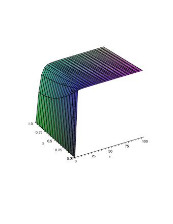
Figure 1: The evolution of temperature $u$

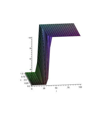
Figure 2: The control $\beta$

With an initial guess for the value of the control, the consecutive values of $\beta$ converge to the lower bound when time is small and to the upper bound when $t$ is big (see Figure 2).

References

- Antontsev and Chipot (1994) S. N. Antontsev and M. Chipot, The thermistor problem: existence, smoothness uniqueness, blowup, SIAM J. Math. Anal. 25 (1994), no. 4, 1128–1156.
- Arantes and Muñoz Rivera (2010) S. F. Arantes and J. E. Muñoz Rivera, Optimal control theory for ambient pollution, Internat. J. Control 83 (2010), no. 11, 2261–2275.
- Cimatti (2007) G. Cimatti, Optimal control for the thermistor problem with a current limiting device, IMA J. Math. Control Inform. 24 (2007), no. 3, 339–345.
- Cimatti (2011) G. Cimatti, Remarks on the existence, uniqueness and semi-explicit solvability of systems of autonomous partial differential equations in divergence form with constant boundary conditions, Proc. Roy. Soc. Edinburgh Sect. A 141 (2011), no. 3, 481–495.
- El Hachimi and Sidi Ammi (2005) A. El Hachimi and M. R. Sidi Ammi, Existence of global solution for a nonlocal parabolic problem, Electron. J. Qual. Theory Differ. Equ. 2005 (2005), no. 1, 9 pp.
- Fowler et al. (1992) A. C. Fowler, I. Frigaard and S. D. Howison, Temperature surges in current-limiting circuit devices, SIAM J. Appl. Math. 52 (1992), no. 4, 998–1011.
- Hömberg et al. (2009/10) D. Hömberg, C. Meyer, J. Rehberg and W. Ring, Optimal control for the thermistor problem, SIAM J. Control Optim. 48 (2009/10), no. 5, 3449–3481.
- Hrynkiv (2009) V. Hrynkiv, Optimal boundary control for a time dependent thermistor problem, Electron. J. Differential Equations 2009 (2009), no. 83, 22 pp.
- Hrynkiv et al. (2008) V. Hrynkiv, S. Lenhart and V. Protopopescu, Optimal control of a convective boundary condition in a thermistor problem, SIAM J. Control Optim. 47 (2008), no. 1, 20–39.
- Kwok (1995) K. Kwok, Complete guide to semiconductor devices, McGraw-Hill, New york, 1995.
- Lacey (1995) A. A. Lacey, Thermal runaway in a non-local problem modelling Ohmic heating. II. General proof of blow-up and asymptotics of runaway, European J. Appl. Math. 6 (1995), no. 3, 201–224.
- Ladyzenskaya et al. (1971) O. A. Ladyzenskaya, V. A. Solonikov and N. N. Uralceva, Linear and quasilinear equations of parabolic type, Trans. Math. Monographs, Vol. 23, Amer. Math. Soc., Providence, RI, 1971.
- Lee and Shilkin (2005) H.-C. Lee and T. Shilkin, Analysis of optimal control problems for the two-dimensional thermistor system, SIAM J. Control Optim. 44 (2005), no. 1, 268–282.
- Lions (1969) J.-L. Lions, Quelques méthodes de résolution des problèmes aux limites non linéaires, Dunod, 1969.
- Lions (1971) J.-L. Lions, Optimal control of systems governed by partial differential equations, Translated from the French by S. K. Mitter. Die Grundlehren der mathematischen Wissenschaften, Springer, New York, 1971.
- Maclen (1979) E. D. Maclen, Thermistors, Electrochemical publication, Glasgow, 1979.
- Nikolopoulos and Zouraris (2008) C. V. Nikolopoulos and G. E. Zouraris, Numerical solution of a non-local elliptic problem modeling a thermistor with a finite element and a finite volume method, in Progress in industrial mathematics at ECMI 2006, 827–832, Math. Ind., 12 Springer, Berlin, 2008.
- Rodrigues (1992) J.-F. Rodrigues, A nonlinear parabolic system arising in thermomechanics and in thermomagnetism, Math. Models Methods Appl. Sci. 2 (1992), no. 3, 271–281.
- Shi et al. (1993) P. Shi, M. Shillor and X. Xu, Existence of a solution to the Stefan problem with Joule’s heating, J. Differential Equations 105 (1993), no. 2, 239–263.
- Sidi Ammi (2007) M. R. Sidi Ammi, Optimal control for a nonlocal parabolic problem resulting from thermistor system, Int. J. Ecol. Econ. Stat. 9 (2007), no. F07, 116–122.
- Sidi Ammi (2010) M. R. Sidi Ammi, Application of the -energy method to the non local thermistor problem, Arab. J. Sci. Eng. Sect. A Sci. 35 (2010), no. 1D, 1–12.
- Sidi Ammi and Torres (2007) M. R. Sidi Ammi and D. F. M. Torres, Necessary optimality conditions for a dead oil isotherm optimal control problem, J. Optim. Theory Appl. 135 (2007), no. 1, 135–143. arXiv:math/0612376
- Sidi Ammi and Torres (2008) M. R. Sidi Ammi and D. F. M. Torres, Numerical approximation of the thermistor problem, Int. J. Math. Stat. 2 (2008), no. S08, 106–114. arXiv:0711.0597
- Tröltzsch (2010) F. Tröltzsch, Optimal control of partial differential equations, translated from the 2005 German original by Jürgen Sprekels, Graduate Studies in Mathematics, 112, Amer. Math. Soc., Providence, RI, 2010.
- Tzanetis (2002) D. E. Tzanetis, Blow-up of radially symmetric solutions of a non-local problem modelling Ohmic heating, Electron. J. Differential Equations 2002 (2002), no. 11, 26 pp.
- Zeidler (1988) E. Zeidler, Nonlinear functional analysis and its applications. IV, Translated from the German and with a preface by Juergen Quandt, Springer, New York, 1988.
- Zhou and Liu (2010) J. Zhou and B. Liu, Optimal control problem for stochastic evolution equations in Hilbert spaces, Internat. J. Control 83 (2010), no. 9, 1771–1784.
- Zhou and Westbrook (1997) S. Zhou and D. R. Westbrook, Numerical solutions of the thermistor equations, J. Comput. Appl. Math. 79 (1997), no. 1, 101–118.