Probing the physical and chemical structure of the CS core in LDN 673. Multitransitional and continuum observations

Abstract

High-angular resolution observations of dense molecular cores show that these cores can be clumpier at smaller scales, and that some of these clumps can also be unbound or transient. The use of chemical models of the evolution of the molecular gas provides a way to probe the physical properties of the clouds. We study the properties of the clump and inter-clump medium in the starless CS core in LDN 673 by carrying out a molecular line survey with the IRAM 30-m telescope toward two clumps and two inter-clump positions. We also observed the 1.2-mm continuum with the MAMBO-II bolometer at IRAM. The dust continuum map shows four condensations, three of them centrally peaked, coinciding with previously identified sub-millimetre sources. We confirm that the denser clump of the region, $n\sim 3.6\times 10^{5}$ cm^-3, is also the more chemically evolved, and it could still undergo further fragmentation. The inter-clump medium positions are denser than previously expected, likely $n\sim 1\times 10^{3}$–1$\times 10^{4}$ cm^-3 due to contamination, and are chemically young, similar to the gas in the lower density clump position. We argue that the density contrast between these positions and their general young chemical age would support the existence of transient clumps in the lower density material of the core. We were also able to find reasonable fits of the observationally derived chemical abundances to models of the chemistry of transient clumps.

1 Introduction

It has been long known that molecular clouds are highly structured (e.  g., Blitz & Stark, 1986) and their structure is greatly affected by the motions induced by supersonic turbulence (e. g., Scalo et al., 1998), self-gravity of the gas and magnetic fields inside the clouds (McKee & Ostriker, 2007; Kainulainen et al., 2009). All these processes control the formation and evolution of the density enhancements, of different scale sizes and densities, such as the cores and clumps that will finally give birth to stars. But there are still great uncertainties to identify the connection between starless cores and protostars (Johnstone et al., 2000; Smith et al., 2008). Starless cores are not all the same, despite their overall similarity in structure (Keto & Caselli, 2008), and differences in total mass, density and temperature might account for the differences in dynamical properties, structure, and future evolution of starless cores (Keto & Field, 2005; Keto & Caselli, 2008).

Higher-angular resolution observations are also finding that dense cores in molecular clouds that appeared homogeneous in single-dish observations, are clumpier at smaller scales (Peng et al., 1998; Morata et al., 2003), showing structures as small as 0.02 pc, and masses as low as 0.01$M_{\sun}$. Many of these smaller clumps are unbound and/or showing evidence of being transient (Peng et al., 1998; Morata et al., 2005), and will never be able to form low-mass stars or even brown dwarfs. The mix of bound and unbound structures in dense cores is also found in several regions, such as the Pipe Nebula, where recent molecular line and continuum observations (Lombardi et al., 2006; Muench et al., 2007; Rathborne et al., 2008; Frau et al., 2010) found numerous cores more than 100, most of which appear to be pressure confined, and gravitationally unbound (Lada et al., 2008).

Observations of the emission of molecular lines at millimetre and sub-millimetre wavelengths in cloud cores combined with the modelling of the chemistry of the gas provides a way of obtaining information on the physical structure and the chemical and physical evolutionary stages of the cores. We proposed a time-dependent chemical model that also explored the consequences of the presence of unresolved and transient structures in the gas that would form and disperse in a timescale of $\sim 1$–2 Myrs (Taylor et al., 1996), in order to explain the systematic differences between CS and NH₃ lines (Pastor et al., 1991; Morata et al., 1997). Simulations of the evolution of these cores (Garrod et al., 2005; Garrod et al., 2006) find that clouds that are ensembles of such transients have a clearly different chemistry from a ‘traditional’ static cloud. The gas chemistry appears to be “young” at all times, and the re-cycling of the material frozen out onto dust grains produces a general molecular enrichment of the clouds, even after re-expansion of the transient structures. The background gas in which these inhomogeneities are embedded would be fairly diffuse, but chemically enriched. These chemical enhancements might also account for the variety of chemistries observed in diffuse clouds.

We carried out interferometric high-angular resolution observations of several molecules (CS, HCO⁺  and N₂H⁺) (Morata et al., 2003, hereafter MGE03), which we later combined with single-dish intermediate-angular resolution maps (Morata et al., 2005, from now on MGE05) towards the starless CS core in LDN 673 ($d=300$ pc), in order to test the predictions of the chemical models. The combined single-dish and interferometer maps showed emission of both background and clumped gas, with a clear segregation of clump properties between the northern and southern halves of our observed region, and allowed us to identify 15 resolved clumps in our data cube. The derived clump masses are well below the virial mass, which would point to their being transient, except for the more massive one, which might have a mass, $\sim 1$$M_{\sun}$, closer to the virial mass. The starless core appears to be constituted by a heterogeneous medium of condensations, of various densities and at different stages of chemical evolution, in agreement with theoretical studies that postulate the existence of transient clumps or the transient nature of dense cores generated by dynamical flows within molecular clouds (see e.  g., Falle & Hartquist, 2002; Vázquez-Semadeni et al., 2005; Van Loo et al., 2008). Recently, Whyatt et al. (2010) also found evidence of a heterogeneous medium in scales of less than 0.1 pc near HH objects, as traced by strong HCO⁺ (3-2) emission. These clumps would have gas volume densities $\ga 3\times 10^{4}$ cm^-3.

Table 1: Lines observed with the 30-m IRAM telescope

Transition	Frequency	HPBW	$B_{\mathrm{eff}}$
	(GHz)	(arcsec)
CCH 1–0 $\frac{3}{2}$–$\frac{1}{2}$ $F$=2–1	087.316925	28	0.78
CCH 2–1 $\frac{5}{2}$–$\frac{3}{2}$ $F$=3–2	174.663222	14	0.64
CCH 3–2 $\frac{7}{2}$–$\frac{5}{2}$ $F$=4–3	262.004260	09	0.46
CN 1–0 $\frac{3}{2}$,$\frac{5}{2}$–$\frac{1}{2}$,$\frac{3}{2}$	113.490982	22	0.74
CN 2–1 $\frac{5}{2}$,$\frac{7}{2}$–$\frac{3}{2}$,$\frac{5}{2}$	226.874764	11	0.54
CS 5–4	244.935606	10	0.50
$c$-C3H2 $2_{1,2}$–$1_{0,1}$	085.338906	29	0.78
$c$-C3H2 $4_{1,4}$–$3_{0,3}$	150.851899	16	0.68
HCN 3–2	265.886432	09	0.45
H2CO $2_{1,2}$–$1_{1,1}$	140.839515	18	0.70
H2CO $3_{1,3}$–$2_{1,2}$	211.211448	12	0.57
H2CO $3_{1,2}$–$2_{1,1}$	225.697773	11	0.54
H13CO+ 1–0	086.754330	28	0.78
H13CO+ 2–1	173.506782	14	0.64
H13CO+ 3–2	260.255480	10	0.46
NO $\frac{3}{2}$,$\frac{5}{2}$–$\frac{1}{2}$,$\frac{3}{2}$ $\Pi^{+}$	150.176459	16	0.68
NO $\frac{5}{2}$,$\frac{7}{2}$–$\frac{3}{2}$,$\frac{5}{2}$ $\Pi^{+}$	250.436845	10	0.48
SO $3_{2}$–$2_{1}$	099.299905	25	0.76
SO $4_{5}$–$3_{4}$	206.176062	12	0.58
SO $6_{5}$–$5_{4}$	219.949433	11	0.55
SO $7_{6}$–$6_{5}$	261.843756	10	0.46
SO2 $3_{1,3}$–$2_{0,2}$	104.029410	24	0.76
SO2 $7_{1,7}$–$6_{0,6}$	165.225436	15	0.66

Table 2: Coordinates of the positions selected for the spectral line observation.

Position	Counterpart	R.A.(J2000)	Dec. (J2000)
CL1	N2H+ peak	19:20:51.747	11:13:49.50
CL6	CS peak	19:20:50.003	11:14:53.00
ICLN	Inter-clump N	19:20:51.701	11:15:30.00
ICLS	Inter-clump S	19:20:54.501	11:14:10.00

In order to study the properties of the clump and inter-clump gas in the starless CS core in LDN 673, we selected two positions associated with identified clumps (CL1 and CL6) and two positions where the inter-clump gas would be dominant (where we did not detect any clump). A multitransitional survey of several early- and late- type molecules in these positions allows us to sample the chemical composition of the gas and compare it to the predicted different chemistry of the pre- and post-clump gas in the models. We additionally observed the dust continuum emission in LDN 673. The structure of this paper is as follows: in Sect. 2, we describe the IRAM 30-m spectral line and continuum observations. In Sect. 3, we describe the characteristics of the detected spectra and of the dust continuum emission. The analysis of the observational results and the determination of the physical parameters of the gas and dust are shown in Sect. 4. Finally, Sect. 5 contains the discussion of the results of our analysis and how they can be related to the previous observations, the chemistry of the clouds and the structure of the core.

2 Observations

The spectral line observations were carried out in 2005 August using the 30-m IRAM telescope in Granada (Spain). We used the capability of the ABCD multi-receiver system to observe 10 different molecules (and a total of 23 transitions) with just 6 frequency setups in the 3, 2, and 1-mm bands. Table 1 shows the transitions and frequencies observed. We used the VESPA autocorrelator as a spectral backend, which provided a total bandwidth of 80 MHz, and selected a 20 kHz channel spacing for the receiver at 100 GHz, and a 40 kHz channel spacing for the other three receivers. The achieved velocity resolutions range from 0.4 to 0.07 km s^-1 from the 1 to the 3-mm bands. The main-beam efficiencies and the half-power beam widths at the observed frequencies are also listed in Table 1. We used the frequency-switching mode with a 7.9 MHz throw, except for the configuration that observed simultaneously the CCH (1–0), $c$-C₃H₂ ($4_{1,4}$–$3_{0,3}$), H₂CO ($3_{1,2}$–$2_{1,1}$), and SO ($7_{6}$–$6_{5}$) transitions, where we used a 15.8 MHz throw. We obtained system temperatures, in $T_{\textrm{a}}^{*}$ scale, of 85-160 K at 100 GHz, 215–465 K at 150 GHz, 230–320 K at 230 GHz, and 470–680 K at 270 GHz. We used the GILDAS package of IRAM to reduce, analyse, and display the spectral data.

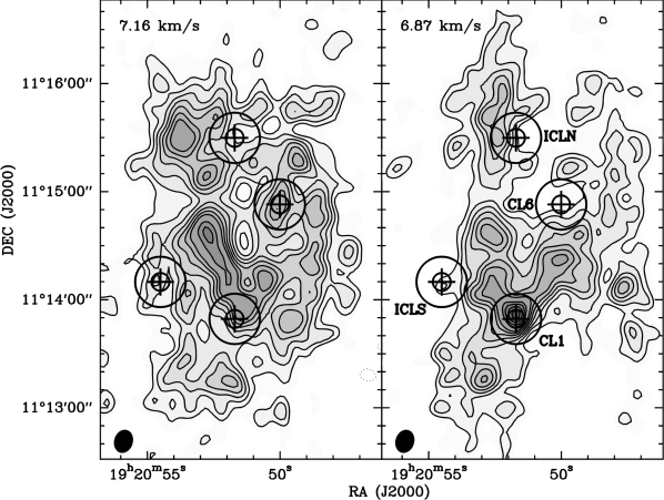
Figure 1: Positions observed with the 30-m telescope in the spectral line observation (crosses) overlapped with the greyscale and contour channel map of the CS (2–1) emission obtained by MGE05. The two concentric circles mark the approximate 30-m beam sizes at 1 and 3 mm, respectively.

Table 2 gives the coordinates and names of the four observed positions. Figure 1 plots the location of the observed positions over the combined BIMA-FCRAO map of the CS ($J$=2$\rightarrow$1) emission of MGE05. The four positions were selected according to the following criteria: (1) two positions centred in two of the CS clumps detected by MGE05: CL1, the most massive and chemically evolved clump, and CL6, a chemically young clump found in the northern region of the BIMA map; (2) two inter-clump positions, one in the northern region (ICLN) and another in the southern region (ICLS), selected from the study of clumpiness of the CS emission in MGE05.

Figure 2: Spectra of the detected transitions of the H₂CO, H¹³CO⁺, CN, $c$-C₃H₂, and CCH molecules at the four selected positions in the CS core of LDN 673, in the velocity range 3–11 km s^-1. The dotted vertical lines indicate the $V_{\mathrm{LSR}}$ of the H₂CO ($3_{1,3}$–$2_{1,2}$) transition for the respective position.

Figure 3: Same as Fig. 2 for the SO, SO₂, NO, and HCN molecules.

Figure 4: Spectra of the detected lines showing hyperfine structure: a) CN, CCH and NO lines at 3-mm; b) CCH (2–1) and CN (2–1) lines in CL1.

The continuum observations were carried out in February 2007 with the 30-m telescope using the MAMBO-II 117-channel bolometer at 1.2 mm. The bolometer effective frequency is 250 GHz and the half-power beam-width at 1.2-mm is $11^{\prime\prime}$. The source was observed using the On-the-fly mode, with a secondary chopping of $42^{\prime\prime}$. The telescope was scanning in azimuth at a speed of $8^{\prime\prime}$ s^-1. Total observation time was 1.4 h, with 57 minutes on source. During the observation, the zenith atmospheric opacity at 225 GHZ was 0.32. The resulting rms was $\simeq 6$ mJy beam^-1. The map was centred at $\alpha\mathrm{(J2000)}=19^{\mathrm{h}}20^{\mathrm{m}}52\aas@@fstack{s}20$; $\delta\mathrm{(J2000)}=11\mbox{${}^{\circ}$}14^{\prime}45\aas@@fstack{\prime\prime}5$ and it covers an effective area of about $9\aas@@fstack{\prime}0\times 6\aas@@fstack{\prime}5$ along the NE–SW direction. We used the MOPSIC package of IRAM to reduce the continuum data and the MIRIAD (Sault et al., 1995) and GILDAS software package to analyse and display the continuum data.

3 Results

3.1 Spectral line observations

Figures 2 and 3 show the spectra obtained in the four selected positions for the detected molecules (19 of the 23 lines observed). Tables 8 to 11 show the line parameters obtained using a Gaussian fit for the transitions detected in the CL1, CL6, ICLN, and ICLS positions, respectively. Table 12 shows the hyperfine structure fit parameters (obtained using the HFS method of the CLASS package) for the detected CN, CCH and NO transitions (Figure 4 shows the full spectra of all the detected hyperfine structure lines). Finally, Table 13 gives the upper limits for the line intensities of the transitions not detected at each position. The CCH (3$\rightarrow$2), CS (5$\rightarrow$4), SO ($7_{6}$$\rightarrow$$6_{5}$), and SO₂ $7_{1,7}$–$6_{0,6}$ lines were not detected at any position. The first three lie in the 1-mm band, which presents higher $T_{\textrm{sys}}$, and typically shows a higher rms than the 3- and 2-mm band values in our spectra.

All the 19 detected transitions are at the CL1 position, whereas the other three positions show detection in 10 (CL6 and ICLN) or 11 (ICLS) transitions. If we compare the intensity for the same line across the four positions, the emission is always more intense at the CL1 position. Lines at the CL6 position tend to be more intense than at ICLS, while lines at the ICLN position are typically the less intense ones.

There are not important differences in the line central velocities among the four positions. The four observed positions show $v_{\rm LSR}$ velocity differences of 0.1–0.2 km s^-1 between them, and are in agreement with the velocity pattern found by MGE05. Linewidths toward CL1 tend to be the narrowest ($\sim 0.4$–0.5 km s^-1, typically). This suggests that the turbulence is lower in CL1 than in the rest of the region.

3.2 Dust continuum emission

Figure 5 shows the 1.2-mm continuum map obtained with the MAMBO-II bolometer. We find four emission condensations with different degrees of extension and intensity. These four condensations were previously detected at 850 $\mu$m by Visser et al. (2002). Table 3 gives the emission parameters derived for these four condensations and the association with the sources of Visser et al. (2002). These four condensations were also recently identified by Tsitali et al. (2010) using the Spitzer Space Telescope, which they classify as starless cores.

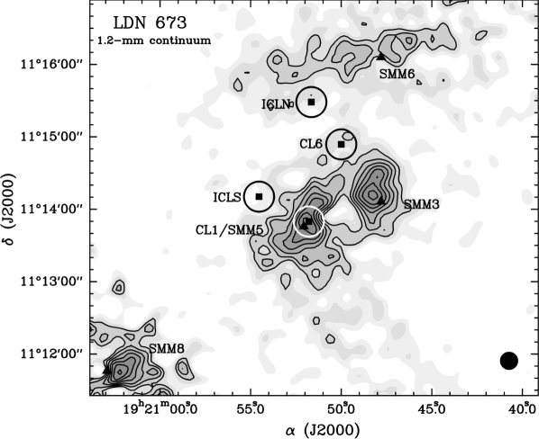
Figure 5: 1.2-mm dust continuum map obtained with the MAMBO-II bolometer after convolving with a $15^{\prime\prime}$ Gaussian beam. The rms noise of the map is 7 mJy beam^-1. The minimum contour is 21 mJy beam^-1, with increments of 7 mJy beam^-1. The circles show the beam size of the 30-m telescope at 3mm, $\sim 25^{\prime\prime}$, centred at each of the positions of the spectral line survey (solid squares). The solid triangles mark the positions of the SMM sources found by Visser et al. (2002).

The three southern condensations show an approximately rounded shape and with centrally peaked emission, whereas the northern condensation rather looks as an extended patch of weak emission. The most intense emission peak (the central clump in Fig. 5), SMM5, coincides with CL1 and with the N₂H⁺ emission of MGE03. Another, slightly smaller, bright condensation is SMM3, with a similar value of the emission peak and located about $\simeq 50^{\prime\prime}$ west of SMM5. A third condensation, again slightly smaller, but with a similar emission peak to the previous two, is SMM8, located $\sim 2\aas@@fstack{\prime}5$ SE of SMM5, near the edge of the 1.2 mm observation’s field of view. This condensation was also detected in H¹³CO⁺ (1–0) and C³⁴S (2–1) in single-dish observations (MGE05). The fourth condensation, associated with SMM6, presents diffuse and extended dust emission in an approximately E–W strip $\sim 2^{\prime}$ north of SMM5 that coincides with a ridge of molecular emission found in an E–W direction in the maps obtained with the FCRAO telescope (MGE05).

Among the four positions observed in spectral lines, only CL1 is associated with a dust peak matching very well with SMM5. CL6 and ICLN are associated with weak dust emission at $2\sigma$, and ICLS is associated with even weaker emission.

4 Analysis

Table 3: Parameters of the condensations found in the 1.2-mm dust emission

			Peak	Fluxa
	Position		intensity	density	FWHMb	Massc	$N(\mathrm{H_{2}})\,$d	$n(\mathrm{H_{2}})\,$d
No.	R.A.(J2000)	DEC.(J200)	( Jy beam-1)	(Jy)	(arcsec)	($M_{\sun}$)	($10^{22}$ cm-2)	($10^{5}$ cm-3)	Association$\,{}^{e}$
1	19:20:46.0	11:16:20.0	0.038	0.436	75	3.9	1.6	0.7	SMM6
2	19:20:48.2	11:14:10.5	0.066	0.253	41	2.9	4.0	3.3	SMM3
3	19:20:52.0	11:13:49.5	0.066	0.339	49	5.1	4.9	3.4	CL1/SMM5
4	19:21:02.4	11:11:43.5	0.065	0.186	35	1.6	3.0	2.8	SMM8

• Flux density integrated above the 2$\sigma$ level after convolving with a 15” Gaussian beam.

• FWHM of the dust emission condensation, $\theta_{\mathrm{FWHM}}=\sqrt{\theta_{s}^{2}-\theta_{b}^{2}}$, where $\theta_{b}$ is the beam-size and $\theta_{s}$ = $2\sqrt{A/\pi}$. $A$ is the area on the map of the pixels with intensity over half of the local continuum emission peak.

• Total mass calculated from the flux density integrated above the 2$\sigma$ level, using the expression from Frau et al. (2010), for a distance of 300 pc.

• $N(\mathrm{H_{2}})$ and $n(\mathrm{H_{2}})$ are the FWHM averaged values of column and volume densities, respectively, calculated using the expressions from Frau et al. (2010), assuming dust temperature, $T_{\mathrm{dust}}=10$ K, a standard dust-to-gas ratio of 100, a dust absorption coefficient at a frequency of 250 GHz, $\kappa_{250}=0.0065$ cm² g^-1 (taken as a medium value between dust grains with thin and thick ice mantles for a volume density of $\sim 10^{5}$ cm^-3, Ossenkopf & Henning (1994), which should be typical for starless cores.

• SMM: sub-millimetre sources from Visser et al. (2002).

4.1 Radiative transfer analysis

The detection of multiple transitions at the same position of some molecules allows us to constrain the physical properties of the emitting gas. We used the RADEX radiative transfer model code (Van der Tak et al., 2007), which treats optical depth effects with an escape probability method, to find the set of molecular column densities, $N(X)$, volume densities, $n$(H₂), and kinetical temperatures, $T_{\mathrm{K}}$, that best reproduced the observed lines. Appendix B gives more details on how the calculations were done.

Table 4: Physical parameters derived from the best-fit model defined by the minimum value of the $\chi^{2}_{\nu}$ function of a series of RADEX models compared to the lines of H₂CO, SO, and H¹³CO⁺ observed in the four positions.

Position	Species	$\theta_{s}$	$T_{K}$	$n(\mathrm{H}_{2})$	$N(\mathrm{X})^{a}$	Transition	$T_{\mathrm{ex}}^{b}$	$\tau^{b}$
		(′′)	(K)	($10^{5}$ cm-3)	(cm-2)		(K)
CL1	H2CO	50	10	3.6	$8.4\times 10^{12}$	$2_{1,2}$–$1_{1,1}$	6.3	1.0
	SO				$4.8\times 10^{13}$	$3_{2}$–$2_{1}$	8.2	2.0
	H13CO+				$8.3\times 10^{11}$	1–0	9.5	0.4
CL6	H2CO	50	10	0.7	$2.8\times 10^{13}$	$2_{1,2}$–$1_{1,1}$	4.7	4.4
	SO				$1.3\times 10^{14}$	$3_{2}$–$2_{1}$	6.7	7.2
	H13CO+				$4.6\times 10^{11}$	1–0	5.0	0.4
ICLN	H2CO	1000	20	0.2	$3.0\times 10^{13}$	$2_{1,2}$–$1_{1,1}$	3.9	3.6
	SO				$6.6\times 10^{13}$	$3_{2}$–$2_{1}$	4.9	2.9
	H13CO+				$4.0\times 10^{11}$	1–0	4.2	0.3
ICLS	H2CO	1000	20	0.2	$2.5\times 10^{13}$	$2_{1,2}$–$1_{1,1}$	4.0	6.1
	SO				$7.6\times 10^{13}$	$3_{2}$–$2_{1}$	5.0	4.9
	H13CO+				$4.0\times 10^{11}$	1–0	3.8	0.5

• Beam-averaged column densities.

• Calculated for the lower frequency transition (the best determined in the observations).

4.1.1 Results of the RADEX analysis: uncertainties

Table 4 shows the best-fit results we obtained from our $\chi_{\nu}^{2}$ analysis using RADEX on the set of lines from the H₂CO, SO, and H¹³CO⁺ molecules, for which at least 3 transitions have been detected at each position. Table 5 shows the best set of parameters that we found for $c$-C₃H₂, HCN, and SO₂, assuming the temperature, volume density and size derived from the previous best fit, plus the results from the hyperfine-line fitting for CCH, CN, and NO.

We estimate that the volume density determination has an uncertainty of 50–70% of the best fit value (shown in Table 4) at the 1-sigma level. The column densities, $N(X)$, are less well constrained than the volume density. The derived column densities of all the molecules have an uncertainty of $\sim 65$% on average from the best-fit value for the CL1 position. For the other positions, the column densities are only constrained within a factor of 2 of the best value.

We alternatively explored how well constrained were the results of our analysis by fixing the H₂CO column density and the filling-factor for each position to the best fit values, and running a range of models with different kinetical temperatures and volume densities. Figure 6 shows the goodness-of-fit over the parameter space spanned by $n(\mathrm{H_{2}}$) and $T_{\mathrm{K}}$. Similarly to the results in Table 4, $n(\mathrm{H_{2}}$) is relatively well-constrained for all positions, but, except for CL1, that is not the case for $T_{\mathrm{K}}$. Temperatures are rather badly determined for the two inter-clump positions, probably due to the lower volume density and the lower SNR of the 1-mm lines. The best fit values of $T_{\mathrm{K}}$ show clear differences between the CL1 and CL6 positions, $T_{\mathrm{K}}\simeq 10$ K, and the inter-clump positions, $T_{\mathrm{K}}\simeq 23$ K (see also Sect. 4.1.2). However, the uncertainties in the inter-clump positions are too large to be significant. We adopt a value of 20 K for the inter-clump gas, since their lower visual extinction may allow the interstellar UV radiation to heat the gas (see e.g., Nejad & Wagenblast, 1999).

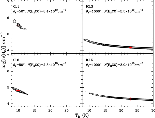
Figure 6: Contours of constant $\chi_{\nu}^{2}$ value (the goodness-of-fit) over the parameter space spanned by the volume density, $n(\mathrm{H_{2}}$), and $T_{\mathrm{K}}$ for fixed values of the H₂CO column density, $N(\mathrm{H_{2}CO}$), for each of the observed positions. The contours mark the confidence levels of 68.3%, 90.0%, and 99.9%. Red (grey) crosses mark the best-fit parameters for each position.

As shown in Fig. 1, the 2 and 3 mm beams of the telescope at both inter-clump positions could have contribution from higher density gas. This effect could be important for the ICLS position, which is the one we studied more carefully (the effect of the emission of CL6 on ICLN is probably very small because the emission in CL6 is much less intense). We used the 1.2-mm continuum map, with an angular resolution $\sim 10\aas@@fstack{\prime\prime}5$, to estimate the contribution to the intensity of the lines at the ICLS position coming from emission from the CL1 position. In order to have an upper limit estimate of the error beam of the telescope at 2 and 3 mm, we convolved the 1.2-mm continuum map with a Gaussian with the same HPBW as the main beam of the telescope at 2 and 3 mm obtained from Greve et al. (1998) and Bensch et al. (2001). Then, we compared the intensities at the clump and inter-clump positions for the original and the convolved maps. We calculated the contribution of the error beam at the CL1 position to the H₂CO, SO, and H¹³CO⁺ lines at the ICLS position as representatives of the different beams we used. We found that the error beam contribution to the molecular line emission in ICLS can be $\la 0.1$–0.5 K, or $\la$18–50% range of the intensity of the detected lines. Thus, though not negligible, we expect a minor contribution of the higher density gas to the lines in the ICLS position. In order to check how much the results of the analysis for the ICLS position can be affected by this contribution, we remade the analysis after subtracting the estimated intensity coming from the CL1 position in the lines measured in ICLS. The resulting number density for ICLS becomes $\sim 3$ times smaller, $\sim 6.6\times 10^{3}$ cm^-3, while the column densities of H₂CO and SO are $\sim 2$ times larger, and H¹³CO⁺ remains practically constant.

4.1.2 Results of the RADEX analysis: volume density, excitation temperature and line opacity

The line intensities and line ratios of our data are best reproduced if we use beam-filling factor and kinetical temperature, $\eta^{i}_{bf}<1$ and $T_{\mathrm{K}}\simeq 10$ K, for CL1 and CL6, but $\eta^{i}_{bf}\simeq 1$ and $T_{\mathrm{K}}\simeq 20$ K give better results for the two “inter-clump” positions. We performed an additional test to check if the “best-values” of the filling-factors are consistent with previous data. From the maps by MGE05, we calculated the main beam antenna temperatures at each of the four positions after convolving the maps with beams of FWHM 14” and 28” and tried to estimate the size of the “apparent” emitting region. The results for the ICLN and ICLS positions agree with $\eta^{i}_{bf}\simeq 1$. For CL1 and CL6, the results agree with $\theta_{s}\sim 30^{\prime\prime}$ and $45^{\prime\prime}$, respectively, not far from the adopted value $\theta_{s}\sim 50^{\prime\prime}$.

The volume densities yielded by the $\chi_{\nu}^{2}$ analysis show a clear distinction between the physical characteristics of the four positions traced by the molecular line emission. The volume density is highest in CL1, $\sim 3.6\times 10^{5}$ cm^-3, $\sim 5$ times larger than the density derived for CL6, and more than one order of magnitude larger than for the inter-clump positions.

Table 5: Physical parameters for the rest of the molecules observed in the four positions of LDN 673 obtained from the best-fit models after fixing $T_{\mathrm{K}}$, $n(\mathrm{H_{2}})$, and $\theta_{s}$ to the values reported in Table 4,

or from the hyperfine structure fitting (see Sect. B.2).

Position	Species	$N(X)\,^{a}$	Transition	$T_{\mathrm{ex}}\,^{b}$	$\tau^{b}$
		(cm-2)		(K)
CL1	$c$-C3H2	$4.5\times 10^{12}$	$2_{1,2}$–$1_{0,1}$	6.5	0.9
	HCN	$1.5\times 10^{13}$	3–2	4.9	6.9
	SO2	$3.7\times 10^{12}$	$3_{1,3}$–$2_{0,2}$	4.5	0.2
CL6	$c$-C3H2	$1.3\times 10^{12}$	$2_{1,2}$–$1_{0,1}$	3.4	0.6
ICLN	$c$-C3H2	$6.0\times 10^{11}$	$2_{1,2}$–$1_{0,1}$	3.3	0.3
ICLS	$c$-C3H2	$1.9\times 10^{12}$	$2_{1,2}$–$1_{0,1}$	3.2	0.9
	SO2	$5.3\times 10^{12}$	$3_{1,3}$–$2_{0,2}$	3.2	0.6
Hyperfine structure calculation
CL1	CCH	$1.7\times 10^{13}$	1–0	5.7	0.3
	CN	$3.4\times 10^{13}$	1–0	4.3	5.9
	NO	$5.3\times 10^{14}$	$\frac{3}{2}$,$\frac{5}{2}$–$\frac{1}{2}$,$\frac{3}{2}$	5.4	0.4
CL6	CCH	$4.7\times 10^{12}$	1–0	4.5	0.1
	CN	$9.1\times 10^{12}$	1–0	3.3	1.4
	NO	$2.2\times 10^{14}$	$\frac{3}{2}$,$\frac{5}{2}$–$\frac{1}{2}$,$\frac{3}{2}$	7.1	$<0.1$
ICLN	CCH	$5.3\times 10^{12}$	1–0	4.1	0.1
	CN	$7.3\times 10^{12}$	1–0	3.1	1.1
	NO	$1.7\times 10^{14}$	$\frac{3}{2}$,$\frac{5}{2}$–$\frac{1}{2}$,$\frac{3}{2}$	5.0	0.1c
ICLS	CCH	$7.0\times 10^{12}$	1–0	3.9	0.2
	CN	$1.1\times 10^{13}$	1–0	3.0	2.2
	NO	$2.5\times 10^{14}$	$\frac{3}{2}$,$\frac{5}{2}$–$\frac{1}{2}$,$\frac{3}{2}$	5.2	0.1c

• Beam-averaged column densities.

• Calculated for the lower frequency transition (the best determined in the observations).

• Calculated after fitting the spectra assuming optically thin lines.

Table 4 also shows the values of excitation temperatures, $T_{\mathrm{ex}}$, and line opacities, $\tau$, yielded by the “best-fit” models for each position and molecule: H₂CO ($2_{1,2}$–$1_{1,1}$), SO ($3_{2}$–$2_{1}$), and H¹³CO⁺ (1-0). We can see that the H₂CO and SO lines tend to be optically thick or very thick, especially for the CL6, ICLN, and ICLS positions, which is also reflected in apparent larger values of the column density, compared to the ones found at CL1. This effect is possibly due to the lower volume density in CL6, ICLN, and ICLS. The rotational levels involved in the H₂CO and SO lines are not of the fundamental rotational level, which makes them more difficult to populate at lower densities. In order to reproduce the observed line intensities, we need to compensate by using higher column densities (and line opacities). This effect is not seen for the H¹³CO⁺ lines, involving the fundamental rotational level, which are relatively optically thin and with CL1 column densities larger or similar to the ones found at the other positions.

The excitation temperatures derived for the lower frequency transition of the molecules of Table 5 lie in a range $\sim$3–7 K, which is very similar to the values of $T_{\mathrm{ex}}$ previously derived for CS (2–1) and N₂H⁺ (1–0) (MGE03, MGE05). Most of the lines are also relatively optically thin, with a few exceptions.

4.1.3 Results of the RADEX analysis: column density

H₂CO and SO column densities are lowest at CL1, by factors of $\sim 3.0$–3.6 and $\sim 1.4$–2.8, respectively, compared to the other positions, while $N$(H¹³CO⁺) is the largest at CL1 by a factor of $\sim 2$. Both ICLN and ICLS show rather similar values for the column densities of the three molecules.

The column density variations for CCH, $c$-C₃H₂  CN, and NO follow similar trends, with small differences. The CL1 position shows the largest column densities for all these molecules, while ICLS has the second largest column density. Column densities in CL6 tend to be slightly larger or similar to the ones in ICLN. The column density of SO₂, which was only detected in two positions, is also $\sim 50$% larger for ICLS than for CL1.

4.2 Dust continuum emission

We calculated the mass of the molecular gas traced by the dust from the continuum emission flux density (Frau et al., 2010). Table 3 gives the H₂ mass, and H₂ averaged column and volume density contained inside the FWHM contour of each of the four condensations found in the 1.2-mm continuum map, assuming a dust temperature of 10 K.

The calculated masses of the four condensations range from 1.6 $M_{\sun}$ for the SE condensation, which is also the smallest one ($\sim 0.05$ pc), to 5.1 $M_{\sun}$ for the CL1/SMM5 condensation. The H₂ volume densities for the three centrally peaked condensations are rather similar, $\sim 3\times 10^{5}$ cm^-3, which is very close to the value derived for the CL1 position from the spectral line observations. The weaker and more diffuse emission of the SMM6 condensation is reflected in a volume density $\sim 4$ times lower, $7\times 10^{4}$ cm^-3, slightly larger than the value derived for the CL6 position. Interestingly, the condensations associated with CL1/SMM5 and SMM3 have similar extensions ($\sim 0.07$ vs $\sim 0.06$ pc), volume densities, and, to a lesser extent, column densities.

In order to estimate the abundances of the observed molecular species (see Sect. 4.3), we also calculated the H₂ column density traced by the dust continuum emission at the four spectral positions using three different angular resolutions: $27^{\prime\prime}$, $22^{\prime\prime}$ and $17^{\prime\prime}$, corresponding to the angular resolution of the spectral line observations at 3.4, 2.7 and 2.1 mm, respectively (Table 6). We adopted a dust temperature value of 10 K for the four positions, given that because of the lack of any internal heating source and that the densities of the gas seem to be $\ga 10^{4}$ cm^-3 we do not expect higher dust temperatures (Goldsmith, 2010). The column densities at the CL1 position are significantly larger than at the other three positions, by factors of $\sim 3$–4 with respect to CL6 and ICLN, and of $\sim$5–10 with respect to ICLS.

Table 6: H₂ average column density traced by the dust continuum emission on the positions of the spectral line observations for three different beam sizes.

		$N(\mathrm{H_{2}})\,^{a}$
	$T_{\mathrm{dust}}$	$(10^{21}$ cm-2)
Position	(K)	$27^{\prime\prime}$	$22^{\prime\prime}$	$17^{\prime\prime}$
CL1	10	31.1	34.8	40.1
CL6	10	10.8	10.9	10.2
ICLN	10	9.0	9.5	11.2
ICLS	10	6.0	5.5	4.3

• Using the parameters given in note ^c of Table 3.

4.2.1 Comparison of dust and CS emission

We convolved the dust map with the 2-point mosaic response of the BIMA telescope in order to properly compare the CS (2–1) and 1.2 mm dust maps. Figure 7 shows the overlap of the CS (2–1) integrated emission from MGE05 with the convolved dust continuum emission at the same angular resolution, $15^{\prime\prime}$. In general the CS and 1.2 mm emissions are not correlated. For the CL1/SMM5 condensation, the CS emission peak is slightly displaced with respect to the dust emission peak, by $\simeq 2^{\prime\prime}$. The western condensation, SMM3, lies just at the limit of the BIMA primary beam, but it seems to be associated with the CS clump 12 (following MGE05 notation). The other CS clumps found through the CLUMPFIND analysis done by MGE05 do not show any clear dust emission peaks. Some of these clumps in the northern part of the map could be associated with the diffuse dust emission arising from SMM6. More interesting is the existence of CS emission in the central parts of the map with very weak or no dust emission.

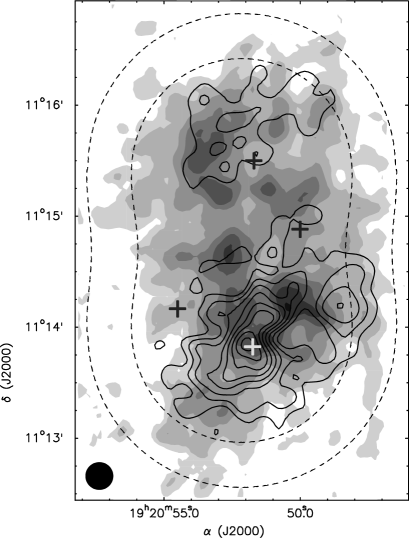
Figure 7: Greyscale of the CS (2-1) integrated emission (from MGE05) overlapped with the contour map of the 1.2 mm dust emission. The angular resolution of both images is $\simeq 15^{\prime\prime}$. The contours of the dust continuum map start at 14 mJy beam^-1with increments of 7 mJy beam^-1; the contours of the CS (2–1) map begin at 0.496 K with increments of 0.248 K. The two maps were convolved with the primary beam response of the BIMA two-point mosaic observations presented by MGE05. The inner and outer dashed lines show the 0.5 and 0.25 level of the BIMA primary beam response. The thick crosses show the four positions observed with the IRAM 30m telescope.

To estimate the CS molecular abundance in the observed BIMA field (see Fig. 7) we first convolved the CS and dust continuum maps with a beam size of 25^′′, in order to measure the dust emission with a higher SNR in the regions where it is diffuse and weak. We then calculated the CS column density assuming LTE conditions, an excitation temperature of $T_{\mathrm{ex}}$=5 K, and a CS (2–1) optical depth line of 3, values derived by MGE05 from multitransitional analysis of the CS and C³⁴S molecules. The H₂ column densities were derived from the dust map adopting a temperature $T_{\mathrm{dust}}$=10 K and dust absorption coefficient of 0.5 cm² g^-1. Figure 8 shows the resulting CS abundance overlapped with the dust emission at the same $25^{\prime\prime}$ angular resolution. The CS abundance changes about one order of magnitude, from $X$(CS)$\sim 10^{-9}$ around the CL1/SMM5 clump to $X$(CS)$\sim 10^{-8}$ about $1^{\prime}$ north of CL1/SMM5, closer to the position of the CL6 CS clump. CS abundances tend to be lower at the positions of the detected dust condensations.

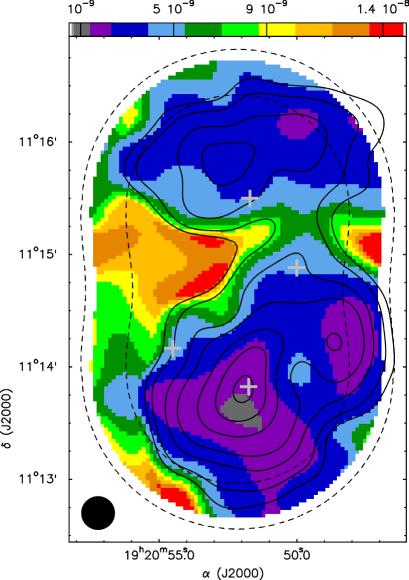
Figure 8: Colour image of the map of the CS abundance, overlapped with the contour map of the 1.2 mm continuum emission. The angular resolution of both images is $25^{\prime\prime}$. The two maps were convolved with the primary beam response of the BIMA two-point mosaic observations presented by MGE05. The inner and outer dashed lines show the 0.5 and 0.25 level of the BIMA primary beam response. The contours are 10%, 15%, 25%, 35%, 55%, 75%, and 95% of the 1.2 mm continuum peak emission, (66.2 mJy beam^-1). The grey crosses show the four positions observed with the IRAM 30m telescope.

4.3 Molecular abundances

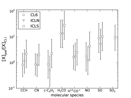
Figure 9: Relative abundances of the molecules detected at the CL6 (circles), ICLN (inverted triangles), and ICLS (squares) positions with respect to the abundance at CL1. The error bars indicate the estimated uncertainties in the determination of the molecular abundances.

For each position, we calculated the molecular abundances of our molecules (Table 7) from the ratio of the beam-averaged molecular column density to the corresponding beam-averaged H₂ column density from Table 6. Taking into account the uncertainties in the calculation of both sets of column densities, we estimate that the uncertainties in the determination of the molecular abundances should be between factors of 2–2.5. For easier comparison, we plotted in Fig. 9 the upper and lower limits that we estimated for the abundances of each molecular species in CL6, ICLN, and ICLS relative to the abundance in CL1.

The abundances of CCH, CN, and $c$-C₃H₂ at CL1 are similar to the values of the other positions, but for the rest of the molecules the abundances are clearly lower, by a factor of $\sim 2$ for H¹³CO⁺ and NO, and of $\sim 10$ for SO, SO₂, and H₂CO. On the other hand, the abundances are systematically larger for all species at ICLS, but only by a factor of $\la 3$ with respect to the abundances at CL6 and ICLN.

Table 7: Molecular abundances calculated from the ratio of the beam-averaged molecular column density to the beam-averaged H₂ column density derived from the dust continuum emission.

Species	Position	Beam$\,{}^{a}$	[X]/[H2]
CCH	CL1	$27^{\prime\prime}$	$5.4\times 10^{-10}$
	CL6		$4.3\times 10^{-10}$
	ICLN		$5.8\times 10^{-10}$
	ICLS		$1.2\times 10^{-9}$
CN	CL1	$22^{\prime\prime}$	$9.9\times 10^{-10}$
	CL6		$8.3\times 10^{-10}$
	ICLN		$7.6\times 10^{-10}$
	ICLS		$2.0\times 10^{-9}$
$c$-C3H2	CL1	$27^{\prime\prime}$	$1.4\times 10^{-10}$
	CL6		$1.2\times 10^{-10}$
	ICLN		$6.7\times 10^{-11}$
	ICLS		$3.2\times 10^{-10}$
HCN	CL1	$12^{\prime\prime}$	$3.0\times 10^{-10}$
H2CO	CL1	$17^{\prime\prime}$	$2.1\times 10^{-10}$
	CL6		$2.7\times 10^{-9}$
	ICLN		$2.7\times 10^{-9}$
	ICLS		$5.8\times 10^{-9}$
H13CO+	CL1	$27^{\prime\prime}$	$2.7\times 10^{-11}$
	CL6		$4.2\times 10^{-11}$
	ICLN		$4.4\times 10^{-11}$
	ICLS		$6.6\times 10^{-11}$
NO	CL1	$17^{\prime\prime}$	$1.3\times 10^{-8}$
	CL6		$2.2\times 10^{-8}$
	ICLN		$1.5\times 10^{-8}$
	ICLS		$5.7\times 10^{-8}$
SO	CL1	$22^{\prime\prime}$	$1.4\times 10^{-9}$
	CL6		$1.2\times 10^{-8}$
	ICLN		$6.9\times 10^{-9}$
	ICLS		$1.4\times 10^{-8}$
SO2	CL1	$22^{\prime\prime}$	$1.1\times 10^{-10}$
	ICLS		$9.6\times 10^{-10}$

• Beam-size over which the molecular and H₂ column densities were averaged.

5 Discussion

5.1 Fragmentation in the core

The most intense emission in the central region of the 1.2-mm dust continuum map is contained inside the HPBW of the low-angular resolution NH₃ map of Sepúlveda et al. (2011). The BIMA observations of MGE03 also only detected N₂H⁺ emission in a region almost coinciding with CL1/SMM5 (the other dust continuum sources lie outside the BIMA primary beam). The dust and N₂H⁺ emissions in CL1/SMM5 are similarly elongated in an approximately N–S direction with a close proximity between both emission peaks. A second clump, located just North of CL1/SMM5 could also be present in the dust emission, but it is not so clearly seen as in the N₂H⁺ map. The sizes of the CL1/SMM5 condensation in the continuum and molecular (CS and N₂H⁺) maps are very similar, $\sim$0.07–0.09 pc, but the gas mass traced by the dust is $\sim$ 4 times larger than the masses estimated, assuming standard abundances, from the CS and N₂H⁺ maps by MGE05.

We showed in Sect. 4.2.1 that the CS and dust emissions do not seem to be particularly correlated (see Figs. 7 and 8): the most intense CS emission around CL1/SMM5 follows the edges of the most intense dust emission and many of the clumps detected in the combined FCRAO and BIMA maps are located in regions with no or very weak dust emission. These results suggest that there is some low density/small-size structure which is revealed by the CS lines, but it is not detected at 1.2-mm, probably because the sensitivity of our observations is not high enough or due to the spatial filtering of the chopping bolometer observations.

The SMM8 dust condensation is also coincident with relatively weaker H¹³CO⁺ and CS emission detected with the FCRAO telescope by MGE05 at the tip of a very weak NW-SE filamentary structure or thin ridge found in the molecular line maps. This filamentary structure is undetected in the dust continuum map.

In order to study the fragmentation in the core, we calculated the Jeans-length corresponding to the densities of the two main dust condensations, CL1/SMM5 and SMM3, following Hartmann (1998):

$$\lambda_{\mathrm{J}}=\left(\frac{\pi a^{2}}{G\rho}\right)^{1/2}=0.19~{}\mathrm{pc}\left(\frac{T}{10\mathrm{K}}\right)^{1/2}\left(\frac{n_{\mathrm{H_{2}}}}{10^{4}\mathrm{cm^{-3}}}\right)^{-1/2}$$ (1)

with the sound speed $a$, the gravitational constant $G$, and the density $\rho$. The separation between the condensations is $\sim 50^{\prime\prime}$, which at the distance of LDN 673 corresponds to $\sim 0.073$ pc ($\sim 15000$ AU). We used the average of the densities estimated for both condensations from the continuum observations, $\sim 3.3\times 10^{5}$ cm^-3, as the volume density, $n_{\mathrm{H_{2}}}$, and assumed $T=10$ K. We obtained a Jeans-length value of $\sim 0.033$ pc, about 2 times smaller than the measured separation on the sky, and similar to the values found by Tsitali et al. (2010) for some other condensations in the region. This value of the Jeans-length is also smaller than the sizes of both condensations, which is an indication that they may still be subject to more thermal fragmentation. Indeed, there is evidence of fragmentation in the CL1/SMM5 condensation, since this clump is associated with two N₂H⁺ condensations separated by $\sim 30^{\prime\prime}$ (MGE05), which corresponds to $\sim 0.044$ pc ($\sim$9000 AU), very close to the Jeans-length previously estimated. On the other hand, most of the CS clumps detected by MGE05 and not traced by the 1.2-mm dust map have typical sizes of 0.04 pc and densities of a few times $10^{4}$ cm^-3. For a density of $7\times 10^{4}$ cm^-3 (the CL6 density), the Jeans-length is 0.07 pc. Thus, these clumps are unlikely to have been formed as a result of thermal fragmentation and we would need to invoke non-thermal processes (turbulence, MHD waves, etc) to explain their existence (Falle & Hartquist, 2002; Vázquez-Semadeni et al., 2005; Klessen et al., 2005; Van Loo et al., 2008). This would agree with the transient nature of this clumps postulated by MGE05.

5.2 The nature of the clumps and the inter-clump medium

The interpretation of single-point observations of molecular lines as the ones presented here have to be taken with caution, because they will never provide the same level of detail of the chemistry as a full map would. However, our choice of positions with presumed different physical conditions, coupled with the dust continuum map, provides us with a sample of molecular abundances that can show some of the properties of our core.

MGE05 already showed that CS was probably depleted in CL1, while N₂H⁺ was clearly centrally condensed. The estimation of the CS abundance in Fig. 8 confirms this result for the SMM5, SMM3, and SMM6 dust condensations. Additionally, Table 7 shows that H₂CO, SO, SO₂, and, to a lesser extent, H¹³CO⁺ are also depleted for CL1 with respect to the abundances at the other positions. On the other hand, the abundances of CCH, $c$-C₃H₂, and CN in CL1 do not seem to differ much from the values in CL6 and ICLN. Finally, the NO abundance at CL1 is also $\sim 40$% lower than the one at CL6, and similarly to what Akyilmaz et al. (2007) found in L1544, the NO molecule could be partially depleted in CL1, while N₂H⁺ is not.

The original models of Taylor et al. (1996, 1998) and Garrod et al. (2005); Garrod et al. (2006) required the action of depletion to obtain the distribution of molecular abundances that would explain the results of MGE03 and MGE05. As has been extensively found in different starless cores, ’early-time’, carbon-bearing molecules, would be depleted in the more central regions of evolved starless cores, wherein ’late-time’, nitrogen-bearing molecules, would still be present in the gas (see e. g., Caselli et al., 1999; Hily-Blant et al., 2010; Tafalla et al., 2006). Thus, the results for CS, N₂H⁺, H₂CO, SO, and H¹³CO⁺ are approximately as expected, given the density of the CL1/SMM5 condensation. However, the low or no depletion of CCH, $c$-C₃H₂, and CN is much more unexpected. Frau et al. (2012) also found a similar result in several cores of the Pipe Nebula, where SO shows depletion, but $c$-C₃H₂ and CCH are more intense in the cores with higher A${}_{\textrm{V}}$.

CL6 and the inter-clump positions show a poorer variety of molecules compared to that of CL1. Additionally, there is little evidence of depletion of the detected molecules – the abundances of early-time molecules are usually the largest in the inter-clump positions – with no detection of N₂H⁺. All this seems to indicate that the gas in CL6, ICLN, and ICLS is chemically young. The gas density in CL6 is more similar to the densities found in the inter-clump medium (see Sect. 4.1.2) than to the density in CL1. However, the number density derived for CL6 is still a factor of $\sim 3.5$ larger with respect to the two inter-clump positions, which indicates that the physical conditions are probably different. This factor is significant and probably a lower limit to the true density contrast, because the probable contribution to the emission from nearby clumps will have the effect of measuring a density higher than the true inter-clump density in ICLN and ICLS (see Sect 4.1.1). In any case, it seems clear that the inter-clump positions are denser than initially expected, probably from a few times $10^{3}$ to $10^{4}$ cm^-3.

5.2.1 Comparison with models of transient clumps

In order to have a more quantitative comparison, we compared the results of our observations to the “standard” model of Garrod et al. (2005); Garrod et al. (2006). We found that this model is able to explain reasonably the chemistry of the CL6 and ICLN positions. However, we used a “high-density” model that reached a higher peak density, $\sim 5.5\times 10^{5}$ cm^-3, in $10^{6}$ yr (Garrod, 2005) to match better the chemistry in CL1. We did not compare the models to ICLS due to the contamination issues discussed in Sect. 4.1.1. We consider that the real evolutionary properties of the gas we observed are probably between these two models and some scaling of abundances would be needed to really fit our results, which is outside the purpose of this discussion. Given the traditional difficulty of matching the values of chemical models to observations, we looked for the time ranges in which the abundances of most of the molecules in the models ($>70\%$) were within a factor of 3 from the observed values, in order to account for the multiple sources of uncertainties in both observations and models.

The molecular abundances in CL1 are compatible with a clump in the “high-density” model in a time range of 3–7$\times 10^{5}$ yr. HCO⁺ is the main outlier, depending on the ¹²C/¹³C abundance ratio used, and “late-time” molecules, NO and SO, tend to push the time range to later times. The abundances in CL6 are better reproduced with a clump following the standard model at times either 5–9$\times 10^{5}$ yr or 1.4–$1.6\times 10^{6}$ yr. So, the clump in CL6 could be very close to the peak density maximum or just past it in the dissipation phase. We also found that the results for ICLN could be compatible with a clump of 0.9–1.6$\times 10^{6}$ yr for the standard model. This could explain the relatively low contrast in density between CL6 and ICLN, if we think that the gas in ICLN could be the remains of a clump that has almost dispersed and what we found was lower density gas enriched by the molecular abundances of previous stages. This would reinforce one of the predictions of Garrod et al. (2006) models: that the formation and dispersion of transient clumps would result in a chemistry of the gas generally “young”, except in the denser and more evolved clumps, and a gas chemical composition that would show signs of “enrichment” of abundances of some molecular species in the lower density material.

Garrod et al. (2006) also showed that a distribution of transient clumps at different stages of evolution (different points in time) could qualitatively reproduce the medium- and high-angular resolution maps of MGE03 and MGE05. Our results here suggest that those clumps could not only be in different stages of evolution but also reach different peak densities, i.e. follow different evolutionary patterns. The mix of clumps with different evolutionary properties can shed a different light on the discussion about the molecular depletion between different clumps. We found that, for the times best fitted by the models, the differences in the abundances of CCH, $c$-C₃H₂, and CN between the “high-density” and “standard” models are considerably smaller than for later-time molecules, such as NO. This would simply explain the apparent low or no depletion of the former molecules compared to the latter.

6 Conclusions

We studied the properties of the clump and inter-clump gas in the CS starless core of LDN 673 using the 30-m IRAM telescope through the emission of several spectral lines in the 3-, 2-, and 1-mm bands, in four positions associated with already detected, but physically and chemically different, clump gas (positions CL1 and CL6), or with inter-clump gas (positions ICLN and ICLS). We detected 19 spectral transitions of 10 molecular species at least in one of the four positions. We complemented the spectral observations with the mapping of the 1.2-mm dust continuum emission in LDN 673, which allowed us to obtain a more reliable estimate of the volume density of the gas and of the abundances of the detected molecules. The main results of our study are:

1. The dust continuum observations revealed four emission condensations in the region, roughly coinciding with SMM sources found by Visser et al. (2002), three of them with a round shape and centrally peaked emission: CL1/SMM5 is the most intense and coincides with the N₂H⁺ clump found by MGE03; SMM3, located $\sim 50^{\prime\prime}$ to the West, was not previously found in the molecular observations; and SMM8, located $\sim 2\aas@@fstack{\prime}5$ SE of the centre of the map, and coinciding with an emission enhancement in the C³⁴S and H¹³CO⁺ maps of MGE05. Finally, there is a more diffuse emission strip extended E–W $\sim 2^{\prime}$ north of CL1/SMM5. The masses of these condensations range from 1.6 to 5.1 $M_{\sun}$ and sizes 0.05–0.07 pc. The northern condensation is sensibly more diffuse.

2. We made a radiative transfer analysis using the RADEX code to determine the molecular column densities, volume density, and kinetical temperature at each position. The best fits to our observations found $T_{\mathrm{K}}\simeq 10$ K for the CL1 and CL6, and $\simeq 20$ K for the ICLN and ICLS positions; and volume densities ranging from $\sim 3.6\times 10^{5}$ cm^-3 at CL1 to $\sim 1.7\times 10^{4}$ cm^-3 at ICLS.

3. CL1 presents the largest column densities for most of the molecules (H¹³CO⁺, $c$-C₃H₂, CCH, CN, and NO), but the smaller column densities for H₂CO and SO. The estimated molecular abundances of most of the molecules, are smallest at CL1, while the abundances at CL6 and ICLN tend to be very similar.

4. The comparison of the dust continuum emission to previous interferometer and single-dish observations shows very little or no correlation between the CS (2–1) and the 1.2-mm emission, with most of the clumps found in the CS emission not detected in the continuum observations. On the other hand, the dust continuum and N₂H⁺ emissions are much more similar.

5. We found that the condensations detected in the dust continuum map may be subject to more thermal fragmentation, which might be already happening in CL1/SMM5. However, most of the clumps detected in CS, but undetected in the dust continuum observations, are unlikely to have been formed by thermal fragmentation, and would need other mechanisms to explain their formation. These clumps were proposed to be transient by MGE05.

6. The chemistry of CL1 appears to be much more evolved than for the other positions, with signs of depletion of several molecular species (CS, H₂CO, SO, H¹³CO⁺, and partially NO), but also relatively unexpected high abundances of CCH, $c$-C₃H₂, and CN. The density contrast between CL6 and the two inter-clump positions, which are denser that initially expected, is relatively low. The gas at the CL6 and inter-clump positions seems to be generally chemically “young”.

In summary, the central condensation, CL1/SMM5, is probably approaching the ’peak-time’ state of the models of Garrod et al. (2005); Garrod et al. (2006) and it is also the place with a larger probability of future undergoing of star formation (see MGE05). The SMM3 condensation is probably in a very similar state, from its shape and gas density, but we cannot firmly determine it until further observations provide us with more information about its chemistry. The low density contrast between CL6 and the inter-clump positions and their similar young chemical age seems to support the idea of the presence of lower density transient clumps in the core as proposed by Garrod et al. (2006).

7 acknowledgements

O.M. is supported by the NSC (Taiwan) ALMA-T grant to the Institute of Astronomy & Astrophysics, Academia Sinica. O.M. acknowledges support from the National Science Foundation (US) while a postdoc at Ohio State University working with Eric Herbst. J.M.G. and R.E. are supported by MICINN grant AYA2008-06189-C03 (Spain). O.M., J.M.G., and R.E. are also supported by AGAUR grant 2009SGR1172 (Catalonia).

Appendix A Line parameters of the observed lines

Tables 8 to 11 show the line parameters obtained using a Gaussian fit for the transitions detected in the CL1, CL6, ICLN, and ICLS positions, respectively. Each table lists the molecular species and transition and the four parameters resulting from the Gaussian fit: line intensity (in main-beam units), central velocity of the line, line-width, and intensity integrated under the Gaussian.

Table 12 shows the hyperfine structure fit parameters, obtained using the HFS method of the CLASS package, for the CN, CCH and NO transitions detected at 3-mm. The table lists: position, molecular species and transition, A$\tau$, central velocity of the hyperfine line of reference, and optical depth of this line.

Finally, Table 13 gives the $3\sigma$ upper limits for the line intensities of the transitions not detected at each position.

Table 8: Line parameters for the transitions detected in Clump 1 (CL1)

	$T_{\mathrm{MB}}$	$V_{\mathrm{LSR}}$	$\Delta V$	Line area
Transition	(K)	(km s-1)	(km s-1)	(K km s-1)
CCH 2–1	$0.35\pm 0.07$	$+7.10\pm 0.04$	$0.48\pm 0.09$	$0.18\pm 0.03$
CN 2–1	$0.79\pm 0.08$	$+7.00\pm 0.01$	$0.41\pm 0.03$	$0.35\pm 0.02$
$c$-C3H2 $2_{0,1}$–$1_{1,2}$	$1.46\pm 0.02$	$+7.16\pm 0.01$	$0.49\pm 0.01$	$0.76\pm 0.01$
$c$-C3H2 $4_{1,4}$–$3_{0,3}$	$0.52\pm 0.06$	$+7.15\pm 0.01$	$0.51\pm 0.03$	$0.28\pm 0.02$
HCN 3–2	$0.88\pm 0.26$	$+6.84\pm 0.03$	$0.28\pm 0.08$	$0.27\pm 0.06$
H2CO $2_{1,2}$–$1_{1,1}$	$1.73\pm 0.06$	$+7.02\pm 0.01$	$0.54\pm 0.02$	$1.00\pm 0.02$
H2CO $3_{1,3}$–$2_{1,2}$	$1.14\pm 0.07$	$+7.00\pm 0.01$	$0.46\pm 0.02$	$0.56\pm 0.03$
H2CO $3_{1,2}$–$2_{1,1}$	$0.75\pm 0.06$	$+7.03\pm 0.01$	$0.41\pm 0.03$	$0.33\pm 0.02$
H13CO+ 1–0	$1.44\pm 0.04$	$+7.23\pm 0.01$	$0.52\pm 0.01$	$0.79\pm 0.02$
H13CO+ 2–1	$1.04\pm 0.15$	$+7.19\pm 0.02$	$0.38\pm 0.06$	$0.42\pm 0.05$
H13CO+ 3–2	$0.39\pm 0.13$	$+7.25\pm 0.03$	$0.23\pm 0.09$	$0.10\pm 0.03$
NO $\frac{5}{2}$,$\frac{7}{2}$–$\frac{3}{2}$,$\frac{5}{2}$	$0.39\pm 0.12$	$+7.14\pm 0.06$	$0.50\pm 0.11$	$0.21\pm 0.05$
SO $3_{2}$–$2_{1}$	$3.45\pm 0.03$	$+7.12\pm 0.01$	$0.52\pm 0.01$	$1.89\pm 0.01$
SO $4_{5}$–$3_{4}$	$0.17\pm 0.04$	$+7.07\pm 0.03$	$0.27\pm 0.06$	$0.05\pm 0.01$
SO $6_{5}$–$5_{4}$	$0.75\pm 0.09$	$+7.03\pm 0.01$	$0.35\pm 0.02$	$0.28\pm 0.02$
SO2 $3_{1,3}$–$2_{0,2}$	$0.19\pm 0.03$	$+7.03\pm 0.03$	$0.42\pm 0.06$	$0.08\pm 0.01$

Table 9: Line parameters for the transitions detected in Clump 6 (CL6)

	$T_{\mathrm{MB}}$	$V_{\mathrm{LSR}}$	$\Delta V$	Line area
Transition	(K)	(km s-1)	(km s-1)	(K km s-1)
$c$-C3H2 $2_{0,1}$–$1_{1,2}$	$0.20\pm 0.01$	$+7.23\pm 0.01$	$0.46\pm 0.03$	$0.10\pm 0.01$
H2CO $2_{1,2}$–$1_{1,1}$	$1.25\pm 0.07$	$+7.16\pm 0.01$	$0.67\pm 0.02$	$0.90\pm 0.03$
H2CO $3_{1,3}$–$2_{1,2}$	$0.77\pm 0.06$	$+7.20\pm 0.01$	$0.56\pm 0.04$	$0.45\pm 0.02$
H2CO $3_{1,2}$–$2_{1,1}$	$0.38\pm 0.05$	$+7.17\pm 0.02$	$0.48\pm 0.06$	$0.19\pm 0.02$
H13CO+ 1–0	$0.51\pm 0.03$	$+7.35\pm 0.01$	$0.60\pm 0.03$	$0.32\pm 0.01$
H13CO+ 3–2	$0.35\pm 0.10$	$+7.35\pm 0.43$	$0.26\pm 0.12$	$0.10\pm 0.04$
SO $3_{2}$–$2_{1}$	$2.87\pm 0.04$	$+7.24\pm 0.01$	$0.52\pm 0.01$	$1.60\pm 0.02$

Table 10: Line parameters for the transitions detected in Inter-clump North (ICLN)

	$T_{\mathrm{MB}}$	$V_{\mathrm{LSR}}$	$\Delta V$	Line area
Transition	(K)	(km s-1)	(km s-1)	(K km s-1)
$c$-C3H2 $2_{0,1}$–$1_{1,2}$	$0.10\pm 0.02$	$+7.27\pm 0.02$	$0.40\pm 0.05$	$0.04\pm 0.01$
H2CO $2_{1,2}$–$1_{1,1}$	$0.79\pm 0.07$	$+7.19\pm 0.02$	$0.95\pm 0.04$	$0.80\pm 0.03$
H2CO $3_{1,3}$–$2_{1,2}$	$0.37\pm 0.06$	$+7.32\pm 0.03$	$0.79\pm 0.08$	$0.31\pm 0.03$
H2CO $3_{1,2}$–$2_{1,1}$	$0.14\pm 0.04$	$+7.34\pm 0.06$	$0.84\pm 0.14$	$0.12\pm 0.02$
H13CO+ 1–0	$0.35\pm 0.02$	$+7.34\pm 0.01$	$0.61\pm 0.03$	$0.23\pm 0.01$
SO $3_{2}$–$2_{1}$	$1.74\pm 0.03$	$+7.23\pm 0.01$	$0.71\pm 0.01$	$1.31\pm 0.01$
SO $6_{5}$–$5_{4}$	$0.18\pm 0.06$	$+7.51\pm 0.07$	$0.50\pm 0.17$	$0.10\pm 0.03$

Table 11: Line parameters for the transitions detected in Inter-clump South (ICLS)

	$T_{\mathrm{MB}}$	$V_{\mathrm{LSR}}$	$\Delta V$	Line area
Transition	(K)	(km s-1)	(km s-1)	(K km s-1)
CN 1–0	$0.26\pm 0.03$	$+7.20\pm 0.10$	$0.65\pm 0.10$	$0.10\pm 0.01$
$c$-C3H2 $2_{0,1}$–$1_{1,2}$	$0.25\pm 0.03$	$+7.27\pm 0.02$	$0.37\pm 0.04$	$0.10\pm 0.01$
H2CO $2_{1,2}$–$1_{1,1}$	$0.90\pm 0.07$	$+7.21\pm 0.01$	$0.46\pm 0.03$	$0.44\pm 0.02$
H2CO $3_{1,3}$–$2_{1,2}$	$0.37\pm 0.05$	$+7.23\pm 0.02$	$0.64\pm 0.06$	$0.25\pm 0.02$
H2CO $3_{1,2}$–$2_{1,1}$	$0.33\pm 0.08$	$+7.24\pm 0.02$	$0.38\pm 0.06$	$0.14\pm 0.02$
H13CO+ 1–0	$0.38\pm 0.02$	$+7.40\pm 0.01$	$0.44\pm 0.02$	$0.18\pm 0.01$
H13CO+ 2–1	$0.24\pm 0.07$	$+7.44\pm 0.06$	$0.36\pm 0.15$	$0.09\pm 0.03$
SO $3_{2}$–$2_{1}$	$1.99\pm 0.03$	$+7.32\pm 0.01$	$0.47\pm 0.01$	$1.00\pm 0.01$
SO2 $3_{1,3}$–$2_{0,2}$	$0.14\pm 0.04$	$+7.23\pm 0.03$	$0.23\pm 0.07$	$0.04\pm 0.01$

Table 12: Line parameters for the transitions with hyperfine structure

		$A\tau$	$V_{\mathrm{LSR}}$	$\Delta V$
Position	Transition	(K)	(km s-1)	(km s-1)	$\tau$
CL1	CCH 1–0	$0.90\pm 0.07$	$+7.19\pm 0.01$	$0.45\pm 0.02$	$0.33\pm 0.29$
	CCH 2–1	$0.88\pm 0.72$	$+7.13\pm 0.02$	$0.28\pm 0.09$	$1.97\pm 2.75$
	CN 1–0	$7.76\pm 0.83$	$+7.09\pm 0.01$	$0.35\pm 0.01$	$5.90\pm 0.83$
	CN 2–1	$0.83\pm 0.18$	$+7.00\pm 0.01$	$0.40\pm 0.03$	$0.13\pm 2.31$
	NO $\frac{3}{2}$,$\frac{5}{2}$–$\frac{1}{2}$,$\frac{3}{2}$	$0.78\pm 0.11$	$+7.09\pm 0.01$	$0.48\pm 0.04$	$0.38\pm 0.28$
CL6	CCH 1–0	$0.16\pm 0.01$	$+7.24\pm 0.02$	$0.58\pm 0.05$	$<0.10$
	CN 1–0	$0.58\pm 0.07$	$+7.24\pm 0.01$	$0.57\pm 0.04$	$1.37\pm 0.38$
	NO $\frac{3}{2}$,$\frac{5}{2}$–$\frac{1}{2}$,$\frac{3}{2}$	$0.36\pm 0.03$	$+7.21\pm 0.02$	$0.54\pm 0.07$	$<0.10$
ICLN	CCH 1–0	$0.12\pm 0.01$	$+7.29\pm 0.02$	$0.76\pm 0.07$	$<0.10$
	CN 1–0	$0.28\pm 0.05$	$+7.22\pm 0.02$	$0.62\pm 0.05$	$1.09\pm 0.47$
	NO $\frac{3}{2}$,$\frac{5}{2}$–$\frac{1}{2}$,$\frac{3}{2}$	$0.17\pm 0.02$	$+7.20\pm 0.04$	$0.64\pm 0.10$	$0.10^{a}$
ICLS	CCH 1–0	$0.22\pm 0.06$	$+7.32\pm 0.02$	$0.50\pm 0.05$	$0.22\pm 0.65$
	NO $\frac{3}{2}$,$\frac{5}{2}$–$\frac{1}{2}$,$\frac{3}{2}$	$0.18\pm 0.03$	$+7.26\pm 0.07$	$0.89\pm 0.22$	$0.10^{a}$

• Obtained after assuming optically thin lines.

Table 13: Line intensity $3\sigma$ upper limits for the transitions not detected

	Position
	CL1	CL6	ICLN	ICLS
	$T_{\mathrm{MB}}$	$T_{\mathrm{MB}}$	$T_{\mathrm{MB}}$	$T_{\mathrm{MB}}$
Transition	(K)	(K)	(K)	(K)
CCH 2–1		$<0.15$	$<0.14$	$<0.20$
CCH 3–2	$<0.72$	$<0.58$	$<0.50$	$<0.72$
CN 2–1		$<0.14$	$<0.12$	$<0.12$
CS 5–4	$<0.19$	$<0.34$	$<0.28$	$<0.29$
$c$-C3H2 $4_{1,4}$–$3_{0,3}$		$<0.13$	$<0.17$	$<0.19$
HCN 3–2		$<0.60$	$<0.52$	$<0.49$
H13CO+ 2–1		$<0.24$	$<0.20$
H13CO+ 3–2			$<0.36$	$<0.37$
NO $\frac{5}{2}$,$\frac{7}{2}$–$\frac{3}{2}$,$\frac{5}{2}$		$<0.43$	$<0.31$	$<0.59$
SO $4_{5}$–$3_{4}$		$<0.10$	$<0.10$	$<0.22$
SO $6_{5}$–$5_{4}$		$<0.31$		$<0.24$
SO $7_{6}$–$6_{5}$	$<0.87$	$<0.45$	$<0.42$	$<0.49$
SO2 $3_{1,3}$–$2_{0,2}$		$<0.14$	$<0.12$
SO2 $7_{1,7}$–$6_{0,6}$	$<0.26$	$<0.35$	$<0.25$	$<0.30$

Appendix B Determination of the best-fit solutions using the RADEX modelling

B.1 Method for multiple-line detected molecules

We used for our calculations the line intensities, $T^{i}_{mb}$, of H₂CO, H¹³CO⁺, and SO, which have at least three observed transitions at each of the four positions. We ran a grid of RADEX models using the following ranges in temperature, volume density, and molecular column density: $T_{\mathrm{K}}$ = 10–30 K; $n$(H${}_{2})=10^{3}$–$10^{7}$ cm^-3; and $N(X)=10^{11}$–$10^{15}$ cm^-2. For each set of temperature, volume density, and column density values, RADEX provides the line intensity for each $i$-transition, $T^{i}_{rx}$. The expected, or calculated, mean beam temperature is given by

$$T^{i}_{calc}=T^{i}_{rx}\eta_{bf}^{i}$$ (2)

where $\eta_{bf}^{i}$ is the beam filling-factor of the $i$-transition. Assuming a 2-D Gaussian distribution for the source emission profile, the filling factor can be expressed as

$$\eta_{bf}^{i}=\frac{\theta_{s}^{2}}{\theta_{s}^{2}+\theta_{mb}^{i~{}2}},$$ (3)

where $\theta_{mb}^{i}$ is the FWHM of the antenna main beam at the frequency of the $i$-transition, and $\theta_{s}$ is the FWHM source size.

We obtained the “best-fit model” after searching for the minimum of the reduced $\chi^{2}$ function (Nummelin et al., 2000), $\chi^{2}_{\nu}$, resulting from comparing the measured and calculated line intensities and line intensity ratios for the three aforementioned molecules:

$$\chi^{2}_{\nu}=\frac{1}{n-p}\sum_{k=1}^{3}\biggl{[}\left(\frac{R^{12k}_{obs}-R^{12k}_{calc}}{\sigma^{r12k}_{obs}}\right)^{2}+~{}~{}~{}~{}~{}~{}~{}~{}$$ (4)

$$\left(\frac{R^{13k}_{obs}-R^{13k}_{calc}}{\sigma^{r13k}_{obs}}\right)^{2}+\left(\frac{T^{1k}_{obs}-T^{1k}_{calc}}{\sigma^{1k}_{obs}}\right)^{2}\biggr{]}$$

where $T^{1k}_{obs}$ is the observed line intensity of the lowest frequency transition (which is usually the best determined) of the $k$ molecule, $R^{ijk}_{obs}$ is the observed line intensity ratio between the $i$- and $j$ transitions of the $k$ molecule, $\sigma^{1k}_{obs}$ is the $1\sigma$ uncertainty associated to the observed line intensity of the lowest frequency of the $k$ molecule, $\sigma^{rijk}_{obs}$ is the uncertainty associated to $R^{ijk}_{obs}$, $n$ is the number of data points and $p$ is the number of free parameters. The $calc$ sub-indexes indicate the equivalent values for the line intensities derived with RADEX. For the undetected transitions, we only included in our calculations the intensities from RADEX that were larger or equal, within errors, than the observed ones.

Since the real size of the emitting area at each position was unknown, we used two sets of values of filling-factors in our analysis: $\eta^{i}_{bf}\simeq 1$, obtained by choosing $\theta_{s}=1000^{\prime\prime}$, and $\eta^{i}_{bf}<1$. For the second case, we tested values between 30^′′, similar to the beam size at 3-mm, and $50^{\prime\prime}$, the deconvolved size of the CL1/SMM5 dust condensation as well as the size of the CL6 clump derived by MGE05.

B.2 Method for the rest of molecules

Following a method similar to the one described in Sect. B.1, but fixing the values of $n(\mathrm{H_{2}})$, $T_{\mathrm{K}}$, and $\theta_{s}$ to the best-fit values determined for each position, we looked for the best set of values of column density, $N$, excitation temperature, $T_{\mathrm{ex}}$, and line opacity, $\tau$ for the rest of molecules.

We did not follow this method for the CCH lines, because the collisional rates for this molecule are still unknown (see e.g., Padovani et al., 2009), nor for the CN and NO transitions, because the RADEX code does not take into account the hyperfine line structure, which in this case ends up underestimating the opacity of the lines. Instead, we calculated $T_{\mathrm{ex}}$ and $\tau$ of the lines from the simultaneous fitting of the hyperfine components. In this last case, we assumed a beam-filling factor, $\eta=1$.

References

- Akyilmaz et al. (2007) Akyilmaz M., Flower D. R., Hily-Blant P., Pineau des Forêts G., Walmsley C. M., 2007, A&A, 462, 221
- Bensch et al. (2001) Bensch F., Panis J.-F., Stutzki J., Heithausen A., Falgarone E., 2001, A&A, 365, 275
- Blitz & Stark (1986) Blitz L., Stark A. A., 1986, ApJ, 300, L89
- Caselli et al. (1999) Caselli P., Walmsley C. M., Tafalla M., Dore L., Myers P. C., 1999, ApJ, 523, L165
- Falle & Hartquist (2002) Falle S. A. E. G., Hartquist T. W., 2002, MNRAS, 329, 195
- Frau et al. (2012) Frau P., Girart J. M., Beltrán M. T., 2012, A&A, 537, L9
- Frau et al. (2010) Frau P., Girart J. M., Beltrán M. T., Morata O., Masqué J. M., Busquets G., Alves F. O., Sánchez-Monge A., Estalella R., Franco G. A. P., 2010, ApJ, 723, 1665
- Garrod (2005) Garrod R. T., 2005, Ph.D. Thesis. University College London, UK
- Garrod et al. (2005) Garrod R. T., Williams D. A., Hartquist T. W., Rawlings J. M. C., Viti S., 2005, MNRAS, 356, 654
- Garrod et al. (2006) Garrod R. T., Williams D. A., Rawlings J. M. C., 2006, ApJ, 638, 827
- Goldsmith (2010) Goldsmith P. F., 2010, ApJ, 557, 736
- Greve et al. (1998) Greve A., Kramer C., Wild W., 1998, A&ASS, 133, 271
- Hartmann (1998) Hartmann L., 1998, Accretion Processes in Star Formation. Cambridge University Press
- Hily-Blant et al. (2010) Hily-Blant P., Walmsley M., Pineau Des Forêts G., Flower D., 2010, A&A, 513, A41
- Johnstone et al. (2000) Johnstone D., Matthews H., Moriarty-Schieven G., Joncas G., Smith G., Gregersen E., Fich M., 2000, ApJ, 545, 327
- Kainulainen et al. (2009) Kainulainen J., Beuther H., Henning T., Plume R., 2009, A&A, 508, L35
- Keto & Caselli (2008) Keto E., Caselli P., 2008, ApJ, 683, 238
- Keto & Field (2005) Keto E., Field G., 2005, ApJ, 635, 1151
- Klessen et al. (2005) Klessen R. S., Ballesteros-Paredes J., Vázquez-Semadeni E., Durán-Rojas C., 2005, ApJ, 620, 786
- Lada et al. (2008) Lada C. J., Muench A. A., Rathborne J., Alves J. F., Lombardi M., 2008, ApJ, 672, 410
- Lombardi et al. (2006) Lombardi M., Alves J. F., Lada C. J., 2006, A&A, 454, 781
- McKee & Ostriker (2007) McKee C. F., Ostriker E., 2007, ARA&A, 45, 565
- Morata et al. (1997) Morata O., Estalella R., López R., Planesas P., 1997, MNRAS, 292, 120
- Morata et al. (2003) Morata O., Girart J. M., Estalella R., 2003, A&A, 397, 181
- Morata et al. (2005) Morata O., Girart J. M., Estalella R., 2005, A&A, 435, 113
- Muench et al. (2007) Muench A. A., Lada C. J., Rathborne J. M., Alves J. F., M. L., 2007, ApJ, 671, 1820
- Nejad & Wagenblast (1999) Nejad L. A. M., Wagenblast R., 1999, A&A, 350, 204
- Nummelin et al. (2000) Nummelin A., Bergman P., Hjalmarson A., Friberg P., Irvine W. M., Millar T. J., Ohishi M., Saito S., 2000, ApJS, 128, 213
- Ossenkopf & Henning (1994) Ossenkopf V., Henning T., 1994, A&A, 291, 943
- Padovani et al. (2009) Padovani M., Walmsley C. M., Tafalla M., Galli D., Müller H. S. P., 2009, A&A, 505, 1199
- Pastor et al. (1991) Pastor J., Buj J., Estalella R., López R., Anglada G., Planesas P., 1991, A&A, 252, 320
- Peng et al. (1998) Peng R., Langer W. D., Velusamy T., Kuiper T. B. H., Levin S., 1998, ApJ, 497, 842
- Rathborne et al. (2008) Rathborne J. M., Lada C. J., Muench A. A., Alves J. F., M. L., 2008, ApJS, 174, 396
- Sault et al. (1995) Sault R. J., Teuben P. J., Wright M. C. H., 1995, in Astronomical Data Analysis Software and Systems IV, ed. R. A. Shaw, H. E. Payne, and J. J. Hayes (San Francisco: Astronomical Society of the Pacific), ASP Conf. Ser., 77, 433
- Scalo et al. (1998) Scalo J., Vázquez-Semadeni E., Chappell D., Passot T., 1998, ApJ, 504, 835
- Sepúlveda et al. (2011) Sepúlveda I., Anglada G., Estalella R., López R., Girart J. M., Yang J., 2011, A&A, 527, A41
- Smith et al. (2008) Smith R. J., Clark P. C., Bonnell I. A., 2008, MNRAS, 391, 1091
- Tafalla et al. (2006) Tafalla M., Santiago-García J., Myers P. C., Caselli P., Walmsley C. M., Crapsi A., 2006, A&A, 455, 577
- Taylor et al. (1996) Taylor S. D., Morata O., Williams D. A., 1996, A&A, 313, 269
- Taylor et al. (1998) Taylor S. D., Morata O., Williams D. A., 1998, A&A, 336, 309
- Tsitali et al. (2010) Tsitali A. E., Bourke T. L., Peterson D. E., Myers P. C., Dunham M. M., Evans N. J., Huard T. L., 2010, ApJ, 725, 2461
- Van der Tak et al. (2007) Van der Tak F. F. S., Black J. H., Schöier F. L., Jansen D. J., van Dishoeck E. F., 2007, A&A, 468, 627
- Van Loo et al. (2008) Van Loo S., Falle S. A. E. G., Hartquist T. W., Barker A. J., 2008, A&A, 484, 275
- Vázquez-Semadeni et al. (2005) Vázquez-Semadeni E., Kim J., M. S., Ballesteros-Paredes J., 2005, ApJ, 618, 344
- Visser et al. (2002) Visser A. E., Richer J. S., Chandler C. J., 2002, AJ, 124, 2756
- Whyatt et al. (2010) Whyatt W., Girart J. M., Viti S., Estalella R., Williams D. A., 2010, A&A, 510, A74