The Physics of Granular Mechanics

Abstract

The hydrodynamic approach to a continuum mechanical description of granular behavior is reviewed and elucidated. By considering energy and momentum conservation simultaneously, the general formalism of hydrodynamics provides a systematic method to derive the structure of constitutive relations, including all gradient terms needed for nonuniform systems. An important input to arrive at different relations (say, for Newtonian fluid, solid and granular medium) is the energy, especially the number and types of its variables.
Starting from a careful examination of the physics underlying granular behavior, we identify the independent variables and suggest a simple and qualitatively appropriate expression for the granular energy. The resultant hydrodynamic theory, especially the constitutive relation, is presented and given preliminary validation.

I Introduction

When unperturbed, sand piles persist forever, demonstrating in plain sight granular media’s ability to sustain shear stresses – an ability that is frequently considered the defining property of solids. On the other hand, when tapped, the same pile quickly degrades, to form a layer (possibly a monolayer) of grains minimizing the gravitational energy. This is typical of liquids. The microscopic reason for this dichotomy is clear: The grains are individually (and ever so slightly) deformed if buried in a pile, which is what sustains the shear stress. When tapped, the grains jiggle and shake, and briefly loose contact with one another. This is why they get rid of some of their deformation – which shows up, macroscopically, as a gradual lost of the static shear stress and a continual flattening of the pile. 

When sand is being sheared at a constant rate, both solid and fluid behavior are operative. First, the grains are being deformed, increasing the shear stress as any solid would. Second, the same shear rate also provokes some jiggling, just as if the grains were lightly tapped.  This leads to a fluid-like relaxation of the shear stress – the larger the shear rate, the stronger the jiggling, and the quicker the relaxation. Note the reason why loading and unloading give different responses (called incremental nonlinearity Kolym-1 ; Kolym-2 ): When being loaded, the solid part of granular behavior increases the stress, while the fluid part decreases it. During unloading, both work in the same direction to reduce the stress.

This entangled behavior, we suspect, lies at the heart of the difficulty modeling sand macroscopically. In addition, there is a “history-dependence” of granular behavior that, being experimentally obvious but conceptually confused and ill-defined, further perplexes the modeler. Obviously, if sand can be characterized, as do other systems, by a complete set of state variables, any history-dependence only indicates that the experiments were run at different values of these variables. This is what we believe happens.

The hydrodynamic theory is a powerful approach to continuum-mechanical description (or macroscopic field theory), pioneered by Landau LL6 and Khalatnikov Khal in the context of superfluid helium. Bei considering energy and momentum conservation simultaneously, and combining both with thermodynamic considerations, this approach is capable of cogently deducing, among others, the proper constitutive relation. Hydrodynamics hydro-1 has since been successfully employed to account for many condensed systems, including liquid crystals  liqCryst-1 ; liqCryst-5 , superfluid ³He he3-1 ; he3-3 ; he3-6 , superconductors SC-1 ; SC-2 ; SC-3 , macroscopic electro-magnetism hymax-1 ; hymax-2 ; hymax-4 and ferrofluids FF-2 ; FF-3 ; FF-8 ; FF-9 . Transiently elastic media such as polymers are under active consideration at present polymer-1 ; polymer-3 ; polymer-4 .

Two steps are involved in deriving the theory hydrodynamically, the first specifies the theory’s structure: Being a function of the state variables, the energy itself is not independent. Nevertheless, the form of the energy density $w(s,\rho)$ is left unspecified in this first step, and the differential equations are given in terms of the energy density $w$, its variables and conjugate variables. [Conjugate variables are the derivatives of the energy with respect to the variables, say temperature $T(s,\rho)\equiv\partial w/\partial s$ and chemical potential $\mu(s,\rho)\equiv\partial w/\partial\rho$ for $s,\rho$, the entropy and mass density]. In a continuum theory, a number of transport coefficients [such as the viscosity $\eta(s,\rho)$ or the heat diffusion coefficient $\kappa(s,\rho)$] are needed to parameterize dissipation and entropy production. Neither is their functional dependence specified.

A theory is unique and useful, of course, only when its energy and transport coefficients are made specific, in a second step. This division is sensible, because the first step is systematic, the second is not. The first starts with clearly spelt-out assumptions based on the basic physics of the system at hand, which is followed by a derivation that is algebraic in nature, and hence rather cogent. The second step is a fitting process – one looks for appropriate expressions, by trial and error, for a few scalar functions that, when embedded into the structure of the theory, will yield satisfactory agreement with the many experimental data.

Starting from the physics of granular deformation and its depletion by jiggling, we have identified the variables and derived the structure of the equations governing their temporal evolution JL6 , calling it gsh, for granular solid hydrodynamics. But our second step is not yet complete, and some proposed functional dependencies are still tentative. The expression for the energy appears quite satisfactory, but our notion of the transport coefficients is still vague. Our final goal is a transparent theory with a healthy mathematical structure that is capable of modeling sand in its full width of behavior, from static stress distribution, via elastoplastic deformation elaPla-1 ; elaPla-2 , to granular flow property at higher velocities Haff-1 ; Haff-2 ; chute-2 ; chute-3 .

II Granular State Variables

In this section, we determine the complete set of granular variables starting from the elementary physics of granular deformation and its depletion by jiggling.

II.1 The Elastic Strain

If a granular medium is sheared, the grains jiggle, roll and slide, in addition to being deformed. Only the latter leads to a reversible energy storage. Therefore, the strain $\varepsilon_{ij}=u_{ij}+p_{ij}$ has two parts, the elastic and plastic one, with the first defined as the part that changes the energy. Hence the energy density $w(u_{ij})$ is a function of the elastic strain $u_{ij}$, which alone we identify as a state variable. For analogy, think of riding a bike on a snowy path, up a steep slope. The rotation of the wheel, containing slip and center-of-mass motion, corresponds to the total displacement $d$. The gravitational energy $w(d_{t})$ of the cyclist and his bike depends only on the center-of-mass movement $d_{t}$, the “elastic” or energy-changing portion here. And the gravitational force on the center of mass is $f_{g}=-\partial w/\partial d_{t}$. Similarly, the elastic stress is $\pi_{ij}=-\partial w(u_{ij})/\partial u_{ij}$. When grains jiggle, granular deformation relax, hence

$$\partial_{t}u_{ij}={\rm v}_{ij}-u_{ij}/\tau,$$ (1)

with the usual elastic term ${\rm v}_{ij}\equiv\frac{1}{2}(\nabla_{i}v_{j}+\nabla_{j}v_{i})$, and a relaxation term $-u_{ij}/\tau$ that accounts for plasticity. [Note because the total strain obeys $\partial_{t}\,\varepsilon_{ij}={\rm v}_{ij}$, the evolution of the plastic strain $p_{ij}\equiv\varepsilon_{ij}-u_{ij}$ is also fixed by Eq (1), and given as $\partial_{t}\,p_{ij}=u_{ij}/\tau$.] To understand how plasticity comes about, consider first the following scenario with $\tau=$ constant. If a granular medium is deformed quickly enough by an external force, leaving little time for relaxation, $\int(u_{ij}/\tau)\,{\rm d}t\approx 0$, we have $u_{ij}\approx\varepsilon_{ij}=\int\,{\rm v}_{ij}{\rm d}t$ and $p_{ij}=0$ right after the deformation. The built-up in elastic energy and stress $\pi_{ij}$ is maximal. If released at this point, the system snaps back toward its initial state, as prescribed by momentum conservation, $\partial_{t}\,(\rho{\rm v}_{i})+\nabla_{j}\pi_{ij}=0$, displaying an elastic, reversible behavior. But if the system is being held still ($\partial_{t}\,\varepsilon_{ij}={\rm v}_{ij}=0$) long enough, the elastic strain $u_{ij}$ will relax, $\partial_{t}u_{ij}=-u_{ij}/\tau$, while the plastic strain grows accordingly, $\partial_{t}p_{ij}=u_{ij}/\tau$. When $u_{ij}$ vanishes, elastic energy $w(u_{ij})$ and stress $\pi_{ij}$ are also gone, implying $\partial_{t}\,(\rho{\rm v}_{i})=0$. The system now stays where it is when released, and no longer returns to its original position. This is what we call plasticity.

However, $1/\tau$ is not a constant in sand: It grows with the jiggling of the grains (as the deformation is lost more quickly) and vanishes if they are at rest. If we quantify the jiggling by the associated kinetic energy, or (via the gas analogy) by a granular temperature $T_{g}$, we could account for this by assuming $1/\tau\sim T_{g}$.

As discussed above, a shear rate would jiggle the grains, giving rise to $T_{g}$. For a constant rate, an expression of the form $T_{g}\sim\sqrt{{\rm v}_{ij}{\rm v}_{ij}}\equiv||{\rm v}_{s}||$ is appropriate [see Eq (13) below]. Inserting $1/\tau=\Lambda||{\rm v}_{s}||$ (with $\Lambda$ the proportionality coefficient) into Eq (1), we obtain the rate-independent expression, $\partial_{t}u_{ij}={\rm v}_{ij}-\Lambda u_{ij}||{\rm v}_{s}||$. Being a function of $u_{ij}$, the stress $\pi_{ij}(u_{ij})$ therefore obeys the evolution equation,

$${\partial_{t}}{\pi_{k\ell}}=M_{k\ell ij}\partial_{t}u_{ij}=M_{k\ell ij}({\rm v}_{ij}-\Lambda u_{ij}||{\rm v}_{s}||),$$ (2)

$$M_{k\ell ij}\equiv{\partial\pi_{k\ell}}/{\partial u_{ij}}\equiv{\partial^{2}w}/{\partial u_{ij}\partial u_{k\ell}},$$

which clearly possesses the structure of hypoplasticity Kolym-1 ; Kolym-2 , a state-of-the-art engineering model originally adopted because sand is incrementally nonlinear, and responds with different stress increases depending on whether the load is being increased (${\rm v}_{ij}>0,\,\,||{\rm v}_{s}||>0$) or decreased (${\rm v}_{ij}<0,\,\,||{\rm v}_{s}||>0$). It is reassuring to see that the realism of hypoplasticity is based on the elementary physics that granular deformation is depleted if the grains jiggle; and it is satisfying to realize that the complexity of plastic flows derives from the simplicity of stress relaxation.

Under cyclic loading of small amplitudes, because the shear rate is not constant, $T_{g}$ oscillates and never has time to grow to its stationary value of $T_{g}\sim||{\rm v}_{s}||$. Therefore, the plastic term $u_{ij}/\tau\sim T_{g}$ remains small, and the system’s behavior is rather more elastic than rendered by Eq (2).

The complete equation for $u_{ij}$ is in fact somewhat more complex, 

$${\rm d}_{t}u_{ij}=(1-\alpha){\rm v}_{ij}-u_{ij}^{*}/\tau-u_{\ell\ell}\,\delta_{ij}/\tau_{1},$$ (3)

$$1/\tau=\lambda T_{g},\quad 1/\tau_{1}=\lambda_{1}T_{g},$$ (4)

where $u_{ij}^{*}$ is the deviatoric (or traceless) part of $u_{ij}$ and ${\rm d}_{t}\equiv\partial_{t}+{\rm v}_{k}\nabla_{k}$. The modifications are: (1) The relaxation time for $u_{ij}^{*}$ and $u_{\ell\ell}$ are different. (2) A shear rate ${\rm v}_{ij}$ yields an elastic deformation rate ${\rm d}_{t}u_{ij}$ that is smaller by the factor of $(1-\alpha)$.

In contrast to strain relaxation $\sim u_{ij}/\tau$ that is irreversible, $\alpha$ accounts for reversible processes (such as rolling). Without relaxation, elastic and total strain are always proportional, and for say $\alpha=2/3$, $u_{ij}$ is a third of $\varepsilon_{ij}$. Circumstances are then reversible and quite analogous to a solid – aside from the fact that one needs to move three times as far to achieve the same deformation. So the physics accounted for by $\alpha$ is akin to that of a lever. [This is also the reason why the stress, or counter-force, is smaller by the same factor, see Eq(19).] Note since any granular plastic motion such as rolling and slipping, be it reversible or irreversible, become successively improbable when the grains are less and less agitated, we expect

$$\alpha(T_{g})\to 0,\text{\quad for\quad}T_{g}\to 0,$$ (5)

implying granular media are fully elastic at vanishing granular temperature.

II.2 Mass, Entropy and Granular Entropy

The energy density $w_{0}(s,\rho)$ of a quiescent Newtonian fluid depend on the entropy density $s$ and mass density $\rho$, both per unit volume. Defining the temperature and chemical potential as $T\equiv\partial w_{0}/\partial s|_{\rho}$ and $\mu\equiv\partial w_{0}/\partial\rho|_{s}$, we note that they can be computed only if the functional dependence of $w_{0}(s,\rho)$ is given. The pressure, a prominent quantity in fluid mechanics, is also a conjugate variable, as it is given by $P\equiv\partial\bar{w}/\partial v$ at constant $sv$, where $v\equiv 1/\rho$ is the specific volume, $\bar{w}\equiv w_{0}v$ the energy per unit mass. Again, $P$ is given once $w_{0}(s,\rho)$ is. (Note it is not independent from $\mu$ and $T$, since it may be written as $P=-w_{0}+Ts+\mu\rho$.)

The conserved energy $w$ depends also on the momentum density $g_{i}=\rho{\rm v}_{i}$, and is generally given as $w=w_{0}+g^{2}/2\rho$. So the complete set of variables is given as $s,\rho$ and $g_{i}$, and the hydrodynamic theory of Newtonian fluids consists of five evolution equations for them. Being a structure of an actual theory, these equations contain $w_{0},P$, also $T,\mu,{\rm v}_{i}\equiv\partial w/\partial g_{i}$. They are closed only when $w_{0}$ is specified. 

In continuum-mechanical theories, the entropy $s$ is not always given the attention it deserves. The basic facts underpinning its importance are: The conserved energy $w$ is, in equilibrium, equally distributed among all degrees of freedom, macroscopic ones such as $\rho,g_{i}$, and microscopic ones such as electronic excitations or phonons (ie, short wave length sound waves). The entropy $s$ is the macroscopic degree of freedom that subsumes all microscopic ones (typically of order $10^{23}$), and accounts for the energy contained in them. Off equilibrium, energy is more concentrated in a few degrees of freedom, typically the macroscopic ones. The one-way, irreversible transfer of energy from the macroscopic to the microscopic ones – in fluid mechanics from $\rho,g_{i}$ to $s$ – is what we call dissipation, and the basic cause for irreversibility. A proper account of dissipation must consider the variable $s$, its conjugate variable $T$, and the entropy production $R$ [with $R/T$ denoting the rate at which entropy is being increased, see Eq (9)]. This remains so for systems (such as granular media) that typically execute isothermal changes.

The energy density of a solid depends on an additional tensor variable, the elastic strain $u_{ij}=\varepsilon_{ij}$, which in crystals is very close to the total strain. The associated conjugate variable $\pi_{ij}\equiv-\partial w_{0}/\partial u_{ij}$ is the elastic stress – where linear elasticity, or $\pi_{ij}\sim u_{ij}$, represents the simplest case. The hydrodynamic theory of solids consists of eleven evolution equations, for the variables $s,\rho,g_{i},u_{ij}$, which in their structure contain the conjugate variables $T,\mu,{\rm v}_{i},\pi_{ij}$.

Displaying solid and liquid behavior, granular media have the same variables – in addition to the one that quantifies granular jiggling, for which a scalar should suffice if the motion is sufficiently random. We call it granular entropy $s_{g}$, and define it to contain all inter-granular degrees of freedom: the stochastic motion of the grains (in deviation from the smooth, macroscopic velocity) and the elastic deformation resulting from collisions. We divide all microscopic degrees of freedom contained in $s$ into the  inner- and inter-granular ones, $s-s_{g}$ and $s_{g}$, with the conjugate variables $T\equiv\partial w_{0}/\partial(s-s_{g})$ and $T_{g}\equiv\partial w_{0}/\partial s_{g}$. Equilibrium is established, when both temperatures are equal, and $s_{g}$ vanishes. (There are overwhelmingly more inner than inter granular degrees of freedom. When all degrees have the same amount of energy, there is practically no energy left in $s_{g}$.) The equilibrium conditions are:

$$s_{g}=0,\quad\bar{T}_{g}\equiv T_{g}-T=0.$$ (6)

As zero is the value $s_{g}$ invariably returns to if unperturbed, it is an energy minimum. Expanding the $s_{g}$-dependent part of the energy $w_{2}\equiv w-w(s_{g}=0)$, we take 

$$w_{2}(s,\rho,s_{g})=s_{g}^{2}/(2\rho b),\quad\bar{T}_{g}\equiv\partial w_{2}/\partial s_{g}|_{s}=s_{g}/\rho b,$$ (7)

with $b(s,\rho)>0$. So the twelve independent variables are: $s,s_{g},\rho,g_{i},u_{ij}$ and the hydrodynamic theory consists of evolution equations for them all, of which six are given by Eq (3). The rest will be given in section III. These equations will contain $w_{0}$ and the conjugate variables: $T,\bar{T}_{g},\mu,{\rm v}_{i},\pi_{ij}$, also the pressure, given as

$$P_{T}\equiv-\partial\bar{w}_{0}/\partial v\equiv-w_{0}+\mu\rho+sT+s_{g}\bar{T}_{g},$$ (8)

with the derivative taken at constant $sv,s_{g}v$ and $u_{ij}$. As we shall see in Eq (24), this is the pressure that accounts for the contribution of agitated grains.

II.3 History Dependence and Fabric Anisotropy

Finally, some remarks about the special role of the density in granular behavior. First, it is quite independent of the compression $u_{\ell\ell}$: Plastic motion rearranges the packaging and change the density by up to 20%, without any elastic compression. Second, the local density only changes if there is some jiggling and agitation of the grains, $\bar{T}_{g}\not=0$. Even when non-uniform, a given density remains forever if the grains are at rest. So, if a pouring procedure produces a density inhomogeneity, this will persist as long as the system is left unperturbed, providing an explanation for the history dependence of static stress distribution. Sometimes, these density inhomogeneities have a preferred direction, say, a density gradient along $\hat{x}$. With density-dependent elastic coefficients, the system will then mimic fabric anisotropy, displaying a stress-distribution reminiscent of an anisotropic medium – even when it consists of essentially round grains and the applied stress is isotropic. Our working hypothesis, given a preliminary validation in section IV.1.3, is that both effects are covered by density inhomogeneities. The static stress of a sand pile is calculated there and compared to experiments for two densities, the first uniform and the second with a reduced core density, which we argue is a result of different pouring procedures, being rain-like and funnel-fed, respectively.

III Granular Solid Hydrodynamics (GSH)

This section presents the remaining six evolution equations. They will be explained but not derived, see JL6 for more details and the complete derivation.

III.1 Entropy Production

The evolution equation for the entropy density $s$ is

$$\partial_{t}s+\nabla_{i}(s{\rm v}_{i}-\kappa\nabla_{i}T)=R/T,$$ (9)

$$R=\eta{\rm v}_{ij}^{*}{\rm v}_{ij}^{*}+\zeta{\rm v}_{\ell\ell}^{2}+\kappa(\nabla_{i}T)^{2}$$ (10)

$$+\gamma\bar{T}_{g}^{2}+\beta(\pi^{*}_{ij})^{2}+\beta_{1}\pi_{\ell\ell}^{2}.$$

Eq (9) is the balance equation for the entropy $s$. It is (with $R$ unspecified) quite generally valid, certainly so for Newtonian fluids and solids. The term $sv_{i}$ is the convective one that accounts for the transport of entropy with the local velocity, and $\kappa\nabla_{i}T$ is the diffusive term that becomes operative in the presence of a temperature gradient. $R/T>0$ is the source term. It vanishes in equilibrium, and is positive-definite off it, to account for the fact that the conserved energy $w$ always goes from the macroscopic degrees of freedom to the microscopic ones, $w\to s$.

The functional dependence of $R$ changes with the system. In liquids, $R$ is fed by shear and compressional flows, and by temperature gradients LL6 , as depicted by the first line of Eq (10). In equilibrium, we have ${\rm v}_{ij},\nabla_{i}T=0$; off it, the quadratic form with positive shear and compressional viscosity, $\eta,\zeta>0$ and heat diffusion coefficient, $\kappa>0$, ensures that the entropy $s$ can only increase. In fact, the terms of the first line are, in an expansion of $R$, the lowest order positive ones that are compatible with isotropy.

The second line of Eq (10), with $\gamma,\beta,\beta_{1}>0$, displays the additional dissipative mechanisms relevant for granular media. As discussed in the introduction, a finite $\bar{T}_{g}$ or $\pi_{ij}$, indicating some jiggling or deformation of the grains, will both relax and give rise to entropy production. Since granular stress $\pi_{ij}$ will not dissipate for $\bar{T}_{g}=0$, we require $\beta,\beta_{1}\to 0$ for $\bar{T}_{g}\to 0$.

Being part of the total entropy, the granular entropy $s_{g}$ obeys a rather similar equation, though it needs to account for a two-step irreversibility, $w\to s_{g}\to s$, the fact that the energy goes from the macroscopic degrees of freedom to the mesoscopic, inter granular ones of $s_{g}$, and from there to the microscopic, inner granular ones of $s$, never backwards,

$$\partial_{t}s_{g}+\nabla_{i}(s_{g}{\rm v}_{i}-\kappa_{g}\nabla_{i}\bar{T}_{g})=R_{g}/\bar{T}_{g},$$ (11)

$$R_{g}=\eta_{g}{\rm v}_{ij}^{*}{\rm v}_{ij}^{*}+\zeta_{g}{\rm v}_{\ell\ell}^{2}+\kappa_{g}(\nabla_{i}\bar{T}_{g})^{2}-\gamma\bar{T}_{g}^{2}.$$ (12)

Eq (11) has the exact same form as Eq (9), so do the first three terms of $R_{g}$. But $R_{g}$ also has a negative contribution. The three positive ones, with $\eta_{g},\zeta_{g},\kappa_{g}>0$, account for $w\to s_{g}$, how shear and compressional flows, and gradients in the granular temperature produce $s_{g}$, the jiggling of the grains. The negative term $-\gamma\bar{T}_{g}^{2}$ accounts for $s_{g}\to s$, how the jiggling turns into heat. There is the same term, though with negative sign, in $R$, because the same amount of energy arriving at $s$ must have left $s_{g}$. As emphasized, all transport coefficients $\eta,\eta_{g},\zeta,\zeta_{g},\kappa,\kappa_{g},\gamma,\beta,\beta_{1}$ are functions of the state variables (which may alternatively be taken as $T,\bar{T}_{g},\rho$, $\pi_{\ell\ell}$ and $\pi_{s}^{2}\equiv\pi_{ij}^{*}\pi_{ij}^{*}$).

In the stationary and uniform limit, for $R_{g}=0$ and $\nabla_{i}T_{g}=0$, macroscopic flows produce the same amount of granular entropy as is leaving, implying

$$\gamma\bar{T}_{g}^{2}=\eta_{g}{\rm v}_{ij}^{*}{\rm v}_{ij}^{*}+\zeta_{g}{\rm v}_{\ell\ell}^{2}.$$ (13)

This is the relation employed to arrive at Eq (2), showing that hypoplasticity holds in the limit of stationary shear rates. Given a shear rate, part of its energy will turn into $s_{g}$, which in turn will leak over to $s$. At the same time, some of the flow’s energy will heat up the system directly, with the ratio of the two dissipative channels parameterized by $\eta/\eta_{g}$ and $\zeta/\zeta_{g}$. In dry sand, $\eta,\zeta$ are probably negligible und shall be neglected below – though they should be quite a bit larger in sand saturated with water: A macroscopic shear flow of water implies much stronger microscopic ones in the fluid layers between the grains, and the dissipated energy contributes to $R$.

Finally, we consider the $\bar{T}_{g}$-dependence of $\eta_{g},\zeta_{g},\gamma$. Expanding them,

$$\eta=\eta_{0}+\eta_{1}\bar{T}_{g},\quad\zeta_{g}=\zeta_{0}+\zeta_{1}\bar{T}_{g},\quad\gamma=\gamma_{0}+\gamma_{1}\bar{T}_{g},$$ (14)

we shall assume $\eta_{0},\zeta_{0}=0$, because

• $R_{g}$ then stays well defined for $\bar{T}_{g}\to 0$, see Eq (12);

• Viscosities typically vanish with temperature;

• This fits the Bagnold scaling;

• For $\gamma_{0}\gg\gamma_{1}\bar{T}_{g}$ and $\gamma_{0}\ll\gamma_{1}\bar{T}_{g}$, respectively, we have from Eq (13), for ${\rm v}_{\ell\ell}=0$,

  $$\bar{T}_{g}=(\eta_{1}/\gamma_{0})\,|{\rm v}_{ij}^{*}|^{2},\quad\bar{T}_{g}=\sqrt{\eta_{1}/\gamma_{1}}\,|{\rm v}_{ij}^{*}|.$$ (15)

  This ensures the existence of an elastic regime at vanishing $\bar{T}_{g}$, see section IV.2.2.

III.2 Conservation Laws

The three evolution equations left to be specified are conservation laws, for mass, energy and momentum,

$$\partial_{t}\rho+\nabla_{i}(\rho{\rm v}_{i})=0,\quad\partial_{t}w+\nabla_{i}Q_{i}=-\rho v_{i}\nabla_{i}\phi,$$ (16)

$$\partial_{t}(\rho{\rm v}_{i})+\nabla_{i}(\sigma_{ij}+\rho{\rm v}_{i}v_{j})=-\rho\nabla_{i}\phi,$$ (17)

where $\phi$ is the gravitational potential (on the earth surface, we have $-\nabla_{i}\phi=G_{i}$, the gravitational constant pointing downwards). Without specifying the fluxes $Q_{i},\sigma_{ij}$, these equations are always valid, quite independent of the system, and express the simple fact that being locally conserved quantities (in the absence of gravitation), energy, momentum and mass obey continuity equations. The basic idea of the hydrodynamic theory is to require the structure of the fluxes $Q_{i},\sigma_{ij}$ to be such that, with the temporal derivatives of the variables given by Eqs (3,9,11,16,17), the thermodynamic relation

$$\partial_{t}w(s,s_{g},\rho,g_{i},u_{ij})=(\partial w/\partial s)\partial_{t}s+(\partial w/\partial s_{g})\partial_{t}s_{g}+(\partial w/\partial\rho)\partial_{t}\rho$$

$$+(\partial w/\partial g_{i})\partial_{t}g_{i}+(\partial w/\partial u_{ij})\partial_{t}u_{ij}$$

$$=T\partial_{t}s+\bar{T}_{g}\partial_{t}s_{g}+\mu\partial_{t}\rho+v_{i}\partial_{t}g_{i}-\pi_{ij}\partial_{t}u_{ij}\quad\,\,$$

is identically satisfied, irrespective of $w$’s functional form. This is a rather confining bit of information, enough to uniquely fix the two fluxes as

$$Q_{i}=(w+P_{T}){\rm v}_{i}+\sigma_{ij}{\rm v}_{j}-\kappa T\nabla_{i}T-\kappa_{g}\bar{T}_{g}\nabla_{i}\bar{T}_{g},$$ (18)

$$\sigma_{ij}=(1-\alpha)\pi_{ij}+(P_{T}-\zeta_{g}{\rm v}_{\ell\ell})\delta_{ij}-\eta_{g}{\rm v}_{ij}^{*},$$ (19)

with $P_{T}$ given by Eq (8), and ${\rm v}_{ij}^{*}$ being the deviatory (or traceless) part of ${\rm v}_{ij}$. (For details of derivation see JL6 .) Although now specified to fit granular physics as codified in Eqs (3,9,11), these are still fairly general results, valid irrespective what concrete form $w$ assumes. Moreover, they also nicely demonstrate the dependence on the number and types of variables: Eliminating $s_{g}$, or equivalently, taking $\bar{T}_{g}=0$, in Eqs (8,18,19), one obtains the solid hydrodynamics.  Further eliminating $u_{ij}$ by taking $\pi_{ij}=0$ leads to the fluid hydrodynamics.

Focusing on the plastic motion, the standard approach (especially the thermodynamic consideration by Houlsby and coworkers, Houlsby ) employs the plastic strain $p_{ij}\equiv\varepsilon_{ij}-u_{ij}$ as the independent variable. Although this starts from the same insight about plastic motion, the connection between elastic strain, stress and energy, so similar in solids and granular media, with formulas that hold for both systems, is lost – or at least too well hidden to be useful, see also the discussion in section IV.3.1.

Enforcing a velocity gradient ${\rm v}_{ij}$, the rate of work being received by the system is $-\sigma_{ij}{\rm v}_{ij}=-[(1-\alpha)\pi_{ij}+P_{T}\delta_{ij}]{\rm v}_{ij}+[\zeta_{g}{\rm v}_{\ell\ell}{\rm v}_{\ell\ell}+\eta_{g}v^{*}_{ij}v^{*}_{ij}]$, see Eq (18). Of these, the terms in the first square brackets, being proportional to the velocity and hence odd under time inversion, are reactive; while those $\sim{\rm v}^{2}$ in the second bracket are even and dissipative. Work received via an odd term will leave if its sign is changed by inverting time’s direction; work received via an even term stays, as happens only with dissipative processes. The reappearance of the same factor $(1-\alpha)$ as in Eq (3) is not an accident, but required by energy conservation. If the same velocity leads to an elastic deformation that is smaller by $(1-\alpha)$, then just as with a lever, the force counteracting this deformation $\sigma_{ij}=(1-\alpha)\pi_{ij}+\cdots$ is smaller by the same factor.

This concludes the derivation of the structure of gsh, or granular solid hydrodynamics, given by Eqs (3,8), (9,10,11,12) and (16,17,18,19).

IV Validation of GSH

The advantage of gsh is two-fold, its clear connection to the elementary granular physics as spelt out in the introduction, and more importantly, the stringency of its structure. It cannot be changed at will to fit experiments, without running into difficulties with general principles. The only remaining liberty is the choice of the functional dependence for the energy and some transport coefficients. As this implies much less wiggle room than with typical continuum-mechanical models, any agreement with experimental data is less designed, “hand-crafted,” and more convincing, especially with respect to the starting physics.

In what follows, we shall fist examine granular statics, for a medium at rest, $T_{g}=0$, then go on to granular dynamics, with enforced flows or stress changes, and some accompanying jiggling, $T_{g}\not=0$. An expression for the conserved energy $w$ will be proposed that, in spite of its relative simplicity, reproduces many important granular features when embedded into gsh. As discussed above Eq (6), we divide $w$ into three parts: the micro-, macro- and mesoscopic ones,

$$w=w_{0}(s,\rho)+[w_{1}(u_{ij},\rho,g_{i})+g^{2}/2\rho]+w_{2}(s_{g},\rho).$$ (20)

The first  accounts for the inner-granular degrees of freedom, all subsumed as heat into the true entropy $s$. We take $w_{0}=\langle E(s)/m\rangle\rho$, where $E(s)$ is the energy of a grain, $m$ its mass, and $\langle\rangle$ denotes the average. The second consists of the contributions from the macroscopic variables of momentum density $g_{i}$ and the elastic strain $u_{ij}$, where $w_{1}$ is given by Eq (21) below. The third, $w_{2}(s_{g},\rho)$ of Eq (7), is further specified in section IV.2.1. It accounts for the inter-granular degrees of freedom, the mesoscaled, strongly fluctuating elastic and kinetic contributions.

IV.1 Granular Statics, $\bf{T_{g}=T}$

Given an energy $w_{1}(u_{ij})$, we can use the stress $\pi_{ij}(u_{ij})\equiv-\partial w_{1}/\partial u_{ij}$ and $u_{ij}=\frac{1}{2}(\nabla_{i}U_{j}+\nabla_{j}U_{i})$ to close the stress balance $\nabla_{j}\pi_{ij}(r_{i})=\rho G_{i}$, and determine $\pi_{ij}(r_{i})$ with appropriate boundary conditions. As this is done without any knowledge of the plastic strain, we may with some justification call this granular elasticity ge-1 .

The relation $u_{ij}=\frac{1}{2}(\nabla_{i}U_{j}+\nabla_{j}U_{i})$ remains valid because of the following reasons: In an elastic medium, the stressed state is characterized by a displacement field from a unique reference state, in which the elastic energy vanishes. Because there is no plastic deformation $U_{i}^{p}$, the total displacement is equal to the elastic one. Circumstances appear at first quite different in granular media. Starting from a reference state, a stressed one is produced by the displacement $U_{i}+U_{i}^{p}$, with typically $U_{i}^{p}\gg U_{i}$. Due to sliding and rolling, $U_{i}^{p}$ is highly discontinuous, but $U_{i}$ remains slowly varying, because the cost in elastic energy would otherwise be prohibitive. Fortunately, $U_{i}^{p}$ is quite irrelevant: We have innumerable reference states, all with vanishing elastic energy and connected to one another by purely plastic deformations. As a result, we can, for any given displacement $U_{i}+U_{i}^{p}$, switch to the reference state that is separated from the original one by $U_{i}^{p}$, and to the stressed one by $U_{i}$. Now, the circumstances are completely analogous to that of an elastic medium.

IV.1.1 Yield Surfaces

An important aspect of granular behavior, in the space spanned by the variables, is the existence of yield surfaces. We take them to be the divide between two regions, one in which stable elastic solutions are possible, the other in which they are not – so the system must flow and cannot come to rest. A natural and efficient way to account for yield is to code it into the energy, a scalar. Given the stress balance, the energy is extremal ge-1 – minimal if convex and maximal if concave. Having the energy being convex within the yield surface, and concave beyond it, any elastic solution that is stable within the surface, will be eager to get rid of the excess energy and become unstable against infinitesimal perturbations beyond it.

IV.1.2 The Elastic Energy $\bf{w_{1}}$

Our present choice for the elastic energy is JL6 ; J-L-1 ; J-L-2 ; J-L-3 ,

$$w_{1}(\rho,u_{ij})={\mathcal{B}}\sqrt{\Delta}\left(2\Delta^{2}/5+{u_{s}^{2}}/\xi\right),$$ (21)

where $\Delta\equiv-u_{\ell\ell}$, $u_{s}^{2}\equiv u^{*}_{ij}u^{*}_{ij}$. The energy $w_{1}$ is convex only for $u_{s}/\Delta\leq\sqrt{2\xi}$, or equivalently $\pi_{s}/P_{\Delta}\leq\sqrt{2/\xi}$ (where $P_{\Delta}\equiv\frac{1}{3}\pi_{\ell\ell}$, $\pi_{s}^{2}\equiv\pi^{*}_{ij}\pi^{*}_{ij}$), which coincides with the Drucker-Prager condition.  Taking $\xi=5/3$ gives a friction angle of about $28^{\circ}$. We further take ${\cal B}={\cal B}_{0}\,{\cal B}_{1}(\rho)\,{\cal C}(\rho,u_{ij})$, where ${\cal B}_{0}$ is a constant, and

$${\cal B}_{1} = \left[(\rho-\rho^{*}_{\ell p})/(\rho_{cp}-\rho)\right]^{0.15},$$ (22)

$$2{\cal C} = 1+\tanh[(\Delta_{0}-\Delta)/\Delta_{1}].$$ (23)

The coefficient ${\cal B}_{1}$ diverges for the “random closed-pack” density, $\rho_{cp}$, and is convex only between $\rho_{cp}$ and the “random loose pack” density $\rho_{\ell p}$. [$\rho^{*}_{\ell p}$ is a constant chosen to yield the right value for $\rho_{\ell p}$ with the relation $\rho_{\ell p}\equiv(11\rho_{cp}+9\rho^{*}_{\ell p})/20$.] It accounts for (1) the lack of elastic solutions for $\rho<\rho_{\ell p}$, when the grains loose contact with one another; (2) the stiffening of granular elasticity with growing density, until it (as an approximation for becoming very large) diverges at $\rho_{cp}$.

With $\Delta_{0},k_{1},k_{2},k_{3}$ being constants, and $\Delta_{0}=k_{1}\rho-k_{2}u_{s}^{2}-k_{3}$, we have ${\cal C}=1$ for $\Delta\ll\Delta_{0}$, and ${\cal C}=0$ for $\Delta\gg\Delta_{0}$. It changes from 1 to 0 in a neighborhood of $\Delta_{1}$ around $\Delta_{0}$, destroying the energy’s convexity there. Taking $\Delta_{0}$ to grow with the density and fall with $u_{s}^{2}$ limits the region of stable elastic solutions to sufficiently small $\Delta$-values, reproducing the virgin consolidation curve and the so-called caps at varying void ratios $e$, see Fig 1.

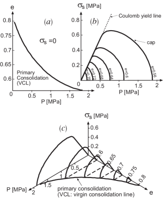
Figure 1: Yield surfaces as coded in the energy of Eqs (21,22,23), a function of the pressure, shear stress, and void ratio. (a): The virgin consolidation line. (b): The bending of the Coulomb yield line, as a function of $e$. (c): Combination of (a) and (b).

IV.1.3 Stress Distribution for Silos, Sand Piles and Point Loads

Three classic cases, a silo, a sand pile and a granular sheet under a point load, are solved employing the stress expression derived from the energy of Eq (21), producing rather satisfactory agreement with experiments.

Silos  For tall silos, the classic approach is given by Janssen, who starts from the assumption that the ratio between the horizontal and vertical stress is constant, $k_{J}=\sigma_{rr}/\sigma_{zz}$. Assuming in addition that $\sigma_{zz}$ only depends on $z$, not on $r$, Janssen finds the vertical stress $\sigma_{zz}$ saturating exponentially with height – a result well verified by observation. (He leaves $\sigma_{rz}$ and all three radial components: $\sigma_{\theta\theta},\sigma_{r\theta}$ and $\sigma_{z\theta}$ undetermined.) Having calculated $\sigma_{zz}$, one needs the value of $k_{J}$ to obtain $\sigma_{rr}$, usually provided by $k_{J}\simeq 1-\sin\varphi$, with $\varphi$ the friction angle measured in triaxial tests. This makes $\varphi$ the only bulk material parameter in silo stress distributions. We shall refer to this as the Jaky formula, although it is also attributed to Kézdi. Being important for the structural stability of silos, this formula is (with a safety factor of 1.2) part of the construction industry standard, see eg. DIN 1055-6, 1987. We believe this formula goes well beyond its practical relevance, that it is a key to understanding granular stresses, because it demonstrates the intimate connection between stress distribution and yield, a connection that has not gained the wide attention it deserves. Starting from Eq (21), we calculated ge-2 all six components of the stress tensor, verifying the Janssen assumptions to within 1%, and found the Janssen constant $k_{J}$ well rendered by the Jaky formula.

Point Loads  The stress distribution at the bottom of a granular layer exposed to a point force at its top is calculated ge-2 employing Eq (21), without any fit parameter. Both vertical and oblique point forces were considered, and the results agree well with simulations and experiments using rain-like preparation. In addition, the stress distribution of a sheared granular layer exposed to the same point force is calculated and again found in agreement with experimental data, see ge-2 for more details and references.

Sand Piles  The fact that the pressure distribution below sand piles and wedges, instead of always displaying a single central peak, may sometimes show a dip, has intrigued and fascinated many physicists, prodding them to think more carefully and deeply about sand. Recent experimental investigations established the following connection: A single peak results when the pile is formed by rain-like pouring from a fixed height; the dip appears when the pile is formed by funneling the grains onto the peak, from a shifting funnel always hovering slightly above the peak. Employing Eq (21) to consider the stress distribution in sand wedges, we found the pressure at the bottom of the pile to show a single central peak if a uniform density is assumed. The peak turns into a pressure dip, if density inhomogeneity, with the center being less compact, is assumed. The two calculated pressure distributions are remarkably similar to the measured ones, see ge-1 . The nonuniform density, we believe, is a consequence of pile formation using the hovering funnel: Since the funnel is always just above the peak, the grains are placed there with very little kinetic energy, resulting in a center region below the peak that has a low density. Those grains that do not find a stable position roll down the slope and gather kinetic energy. When they crash to a stop at the flanks, they compact the surrounding, achieving a much higher density.

IV.2 Granular Dynamics, $\bf{T_{g}\not=T}$

If a granular medium is exposed either to stress changes, or a moving boundary, the grains will flow, displaying both a smooth, macroscopic velocity, ${\rm v}_{i}\not=0$, and some stochastic jiggling, $s_{g}\sim\bar{T}_{g}\not=0$. Then the following effects will come into play: First, the energy is extended by a $s_{g}$-dependent contribution, $w_{2}(s_{g},\rho)$, see Eq (7). Second, the transport coefficients of Eq (14) become finite. Most importantly, third, the relaxation times $\tau,\tau_{1}$ of Eq (3) are no longer infinite, implying the presence of plastic flows.

IV.2.1 The $\bf{s_{g}}$-Dependent Part of the Energy

Specifying the expansion coefficient $b(\rho)$ of Eq (7) as $b=b_{0}(1-\rho/\rho_{cp})^{a}$, we find

$$P_{T}={a\,\rho\,b_{0}\bar{T}_{g}^{2}}{(1-\rho/\rho_{cp})^{a-1}}({\rho}/{2\rho_{cp}})$$ (24)

by employing Eq (8). The density dependence of the expansion coefficient $b(\rho)$ is chosen such that it reproduces the observed volume-dilating pressure contribution $P_{T}\sim f_{2}/(\rho_{cp}-\rho)$ from agitated grains Lub-1 ; Lub-2 ; Lub-3 . However, we cannot take $a=0$ as it would imply a diverging granular entropy $s_{g}$ for $\rho\to\rho_{cp}$. Therefore, we take $a$ to be positiv but small, where $a\approx 0.1$ appears appropriate. (Note that with $w_{0}/\rho$ independent of $\rho$ and $w_{1}/\rho\sim\Delta^{2.5}$ – where $\Delta$ rarely exceeds $10^{-4}$ – the respective density derivative and pressure contribution is zero and negligibly small.)

IV.2.2 The Hypoplastic Regime

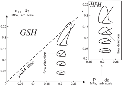
Figure 2: The change in strain ${\rm d}\gamma\equiv({\rm v}_{11}-{\rm v}_{33}){\rm d}t,{\rm d}\varepsilon\equiv-(2{\rm v}_{11}+{\rm v}_{33}){\rm d}t$ for given stress rate starting from different points in the stress space, spanned by $\sigma_{s},P$, as calculated employing (1) gsm, the present theory (taking $1-\alpha=0.22$, $\tau/{\tau_{1}}=0.09$, ${\zeta_{g}}/{\eta_{g}}=0.33$, $\lambda\sqrt{{\eta_{g}}/{\gamma}}=114$), and (2) hpm, a typical hypoplastic model, see JL3 for more figures and details.

We may choose our parameters such that $\bar{T}_{g}$ is small at typical velocities of elasto-plastic deformations, though large enough to cover both limits of Eq (15). Then the first term of Eq (19) dominates, because all other terms ($\sim P_{T},\eta_{g},\zeta_{g}$) are of order $\bar{T}_{g}^{2}$. Then we have $\partial_{t}\sigma_{ij}=(1-\alpha)\partial_{t}\pi_{ij}=(1-\alpha)M_{ijk\ell}\partial_{t}u_{ij}$, with $\partial_{t}u_{ij}$ given by Eq (3). Stress relaxation, the culprit producing irreversible plasticity, is a term $\sim\bar{T}_{g}$. For very slow shear flows and $\bar{T}_{g}\sim||{\rm v}_{ij}||^{2}$ [first of Eq (15)], it is quadratically small and negligible. This is the elastic regime. At somewhat faster shear flows, the relation $\bar{T}_{g}\sim||{\rm v}_{ij}||$ [second of Eq (15)] renders $\partial_{t}\sigma_{ij}$ rate-independent, giving it the basic structure of hypoplasticity, Eq (3). Comparing this results to a state-of-the-art hypoplastic model, we found impressively quantitative agreement, see Fig 2. This is remarkable, because the anisotropy of these figures, determined essentially by $M_{ijk\ell}$, is a calculated quantity: $M_{ijk\ell}\equiv\partial^{2}w_{1}/\partial u_{ij}\partial u_{k\ell}$, with $w_{1}$ given by Eq (21).

IV.2.3 The Butterfly Cycle

Figure 3: Upper row: radial stress $\sigma_{1}$ versus axial stress $\sigma_{3}$, rescaled by $B_{0}\kappa^{-3/2}$. Middle row: radial strain $\varepsilon_{1}=\int{\rm v}_{xx}dt$ versus axial strain $\varepsilon_{3}=\int{\rm v}_{zz}dt$. Lower row: $e-e_{0}$ (with $e_{0}$ the initial void ratio) versus shear strain $\varepsilon_{q}=\int({\rm v}_{zz}-{\rm v}_{xx})dt$, rescaled by $\nu_{1}\kappa$. The stress loads are isobaric for (a) and quasi-isobaric for (b,c); the cyclic amplitude is small for (a,b) and large for (c). The associated strain loci and void ratio are: sawtooth-like for (a), coil-like for (b), butterfly-like (or double-looped) for (c). [The large-amplitude, isobaric plot is quite similar to (c).]

Our last example for validation is not a direct comparison of ghd to some experimental data, but rather an examination of what ghd does, unforced and uncrafted, under typical elasto-plastic deformations. It is solved numerically for stress paths in the triaxial geometry (ie. $\sigma_{xx}=\sigma_{yy}$, $\sigma_{ij}=0$ for $i\neq j$, similarly for $u_{ij}$), including all energy terms given above, except $\mathcal{C}$ of Eq (23) that is set to 1 (assuming the yield surface is sufficiently far away). All transport coefficients depend on $T_{g}$ as specified, but are otherwise constant, independent of stress and density. Also, all variables are taken to be spatially uniform, reducing a set of partial differential equations to ordinary ones in time. In spite of these major simplifications, the results as rendered in Fig 3 display such uncanny realism that it seems obvious gsh has captured some important elements of granular physics. We consider a test with the stress given as

$$P=P^{\text{av}}+P^{\text{ampl}}\cos\left(2\pi ft\right),\quad q=q^{\text{ampl}}\cos\left(2\pi ft+\varphi\right).$$ (25)

Numerical solutions were computed for isobaric test with $P^{\text{ampl}}=0$ (ie. $P=$ constant) and quasi-isobaric test, with $P^{\text{ampl}}<<P^{\text{av}}$ (ie. $P\approx$ constant). The results are shown in Fig 3. they are obtained using the dimensionless parameters: $\kappa\equiv\sqrt{\zeta_{1}\gamma_{1}}/\rho b=18257$, $(\gamma_{0}/\gamma_{1})^{2}$ $(\rho_{cp}b^{2}\kappa^{3/2}/\mathcal{B}_{0}b_{0})=1.07\times 10^{-6}$, $\lambda_{1}/\lambda=0.09$, $\nu_{1}^{2}/2$ $\equiv\eta_{1}/3\zeta_{1}=1$, $\lambda\sqrt{\eta_{1}/\gamma_{1}}=114$, $\alpha=0$. The initial conditions are: $e_{0}=0.68085$ (or $\rho_{0}=0.94\rho_{cp}$), $v_{ij}$, $\bar{T}_{g}$, $\partial_{t}\bar{T}_{g}$, $\partial_{t}\rho$, $\partial_{t}u_{ij}=0$. The averaged pressure $P^{\text{av}}\equiv\sigma_{ii}/3$ is $P^{\text{av}}=70\mathcal{B}_{0}\kappa^{-3/2}$, and the amplitude $q^{\text{ampl}}\equiv\sigma_{3}-\sigma_{1}$ is $5\nu_{1}\kappa^{3/2}q^{\text{ampl}}/6\mathcal{B}_{0}=10$ for (a,b) and $100$ for (c,d). The frequency of $P^{\text{ampl}},q^{\text{ampl}}$ is $f=12(\gamma_{0}/b\rho)$, and the phase lag between them is $\varphi=58^{\circ}$.

IV.3 Competing Concepts and Misconceptions

Finally, we revisit two previous approaches to come to terms with granular behavior, granular thermodynamics by Houlsby et al Houlsby , and granular statistical mechanics by Edwards et al Edw . We shall compare gsh to both assuming at most superficial familiarity with them. Also, we refute some misconceptions that have become unfortunately widespread, especially the one about energy not being conserved in sand [sic]. These are at best a nuisance in exchanges with referees; and at worst actual obstacles in the progress of our coming to grips with granular modeling.

IV.3.1 Granular Thermodynamics

Although considerable work and thoughts have gone into applying thermodynamics to granular media and plastic flow, especially from Houlsby and Collins Houlsby , its basic points are clear and easy to grasp. Taking the entropy production as

$$R=\pi_{ij}\partial_{t}p_{ij}$$ (26)

(where $p_{ij}$ denotes, as before, the plastic strain), it is obvious that the usual linear Onsager force-flux relation, $\partial_{t}p_{ij}\sim\pi_{ij}$, hence $R\sim\pi_{ij}^{2}$, does not give a rate-independent $R$. Therefore, Houlsby, Collins and coworkers consider instead

$$R=\sqrt{\chi_{ijk\ell}\partial_{t}p_{ij}\partial_{t}p_{k\ell}}=(\chi_{ijk\ell}\partial_{t}p_{ij}\partial_{t}p_{k\ell})/{\textstyle\sqrt{\chi_{ijk\ell}\partial_{t}p_{ij}\partial_{t}p_{k\ell}}},$$

a rate-independent expression. Equating it to Eq (26), with $\pi_{ij}=-\partial F/\partial p_{ij}$, and $F$ being the free energy density, one then solves for the plastic strain $p_{ij}$ with a given $F$. One example gives $\partial_{t}p_{ij}\neq 0$ on a yield surface, characterized by some components of $\pi_{ij}$ being constant, and $\partial_{t}p_{ij}=0$ off it.

gsh starts with the same $R$, but possesses the additional variable $T_{g}$, for which $\bar{T}_{g}\sim||{\rm v}_{s}||$ frequently holds, see Eq (13). The linear Onsager force-flux relation

$$\partial_{t}p_{ij}=\beta\pi_{ij}\quad\text{with}\quad\beta\sim\bar{T}_{g},$$ (27)

therefore suffices to yield an rate-independent $R\sim\bar{T}_{g}\pi_{ij}^{2}$. Note Eq (27) leads directly to the relaxation term: Because $\partial_{t}u_{ij}+\partial_{t}p_{ij}={\rm v}_{ij}$, we have $\partial_{t}u_{ij}-{\rm v}_{ij}=-\beta\pi_{ij}=-u_{ij}/\tau$, with $1/\tau\sim\bar{T}_{g}$. (The last equal sign holds because $\pi_{ij},\beta,\tau$ are all functions of $u_{ij}$, with $\beta,\tau$ as yet unspecified.)

Summarizing, without the variable $\bar{T}_{g}$, Houlsby and Collins needed to go beyond the well-verified and -substantiated procedure of linear Onsager force-flux relation to maintain rate-independence, obtaining a plastic flow that is confined to the yield surface. In gsh, rate-independence arises naturally within the confines of linear Onsager relation, producing a plastic flow that is as realistic as hypoplasticity, and finite also off the yield surface.

IV.3.2 Granular Statistical Mechanics

Generally speaking, it is important to remember that of all microscopic degrees of freedom, the inner-granular ones are many orders of magnitude more numerous than the inter-granular ones. It is the former that dominate the entropy and any entropic considerations. When revisiting granular statistical mechanics, especially the Edwards entropy, it is useful to keep this in mind.

Taking the entropy $S(E,V)$ as a function of the energy $E$ and volume $V$, or ${\rm d}S=(1/T){\rm d}E+(P/T){\rm d}V$, the authors of Edw argue that a mechanically stable agglomerate of infinitely rigid grains at rest has, irrespective of its volume, vanishing energy, $E\equiv 0$, ${\rm d}E=0$. The physics is clear: However we arrange these rigid grains that neither attract nor repel each other, the energy remains zero. Therefore, ${\rm d}S=(P/T){\rm d}V$, or ${\rm d}V=(T/P){\rm d}S\equiv X{\rm d}S$. The entropy $S$ is obtained by counting the number of possibilities to package grains for a given volume, and taking it to be $e^{S}$. Because a stable agglomerate is stuck in one single configuration, some tapping or similar disturbances are needed to enable the system to explore the phase space.

In gsh, the present theory, grains are neither infinitely rigid, nor always at rest, hence the energy contains both an elastic and a $s_{g}$-dependent contribution.  And the question is whether granular statistical mechanics is a legitimate limit of gsh. We are not sure, but a yes answer seems unlikely, as both are conceptually at odds in two points, the first more direct, the second quite fundamental: (1) Because of the Hertz-like contact between grains, very little material is being deformed at first, with the compressibility diverging at vanishing compression. This is a geometric fact independent of how rigid the bulk material is. Infinite rigidity is therefore not a realistic limit for sand. (2) As emphasized, the number of possibilities to arrange grains for a given volume is vastly overwhelmed by the much more numerous configurations of the inner granular degrees of freedom, especially phonons. Maximal entropy $S$ for given energy therefore realistically implies minimal macroscopic energy, such that a maximally possible amount of energy is in $S$ (or heat), equally distributed among the inner-granular degrees of freedom. Maximal number of possibilities to package grains for a given volume is a very different criterion.

IV.3.3 Energy Conservation

Stemming ultimately from a loose vocabulary, some alleged difficulties to model sand are based on fallacies that need to be refuted here.

The essential difference between granular gas and ideal (atomic or molecular) gas is that the particles of the first undergo non-elastic, dissipative collisions. As a result, their kinetic energy is not conserved, and the velocity distribution typically lacks the time to arrive at the equilibrium Gaussian form. Quantifying the kinetic energy as a granular temperature $T_{g}$, it is therefore hardly surprising that the fluctuation-dissipation theorem (fdt), formulated in terms of $T_{g}$, is frequently violated. These are sound results, obtained from a healthy but truncated model that takes the grains as the basic microscopic entity with no heat content. However, some of the further conclusions are deduced forgetting this simplification, rendering them patently absurd. These, and their [refutation in italic], are listed below:

• As the energy is not conserved in sand, neither thermodynamics nor the hydrodynamic method are valid. [Only the kinetic energy dissipates in granular media, not the total energy. The latter, including kinetic, elastic and heat contributions, remains conserved – as it is in any other system. And only the conservation of total energy is important for thermo- and hydrodynamics.]

• fdt, along with other general principles either derived from it or in its conceptual vicinity (such as the Onsager reciprocity relation) are all violated. [There are two versions of fdt, only the one given in terms of $T_{g}$ is violated, not the one in terms of the true temperature $T$. The latter is a general principle and always valid. For instance, the volume fluctuation is given as $\langle\Delta V^{2}\rangle=T(\partial^{2}F/\partial V^{2})^{-1}$, with $F$ the associated free energy, for a copper block, a single grain, and a collection of grains. If the grains in the collection are jiggling, there is an extra contribution $\sim T_{g}^{2}$ in $F$, see Eq (7), that considerably increases the value of $\langle\Delta V^{2}\rangle$. The Onsager relation remains valid because the true fdt holds.]

• The Onsager relation is also violated because the microscopic dynamics, the collision of the grains, is dissipative and hence irreversible. [The true microscopic dynamics is that in terms of atoms and molecules, the building blocks of the grains. Their dynamics is, as in any other system, reversible.]

References

- (1) D. Kolymbas, Introduction to Hypoplasticity, (Balkema, Rotterdam, 2000).
- (2) D. Kolymbas, also W. Wu and D. Kolymbas, in Constitutive Modelling of Granular Materials ed D. Kolymbas, (Springer, Berlin, 2000), and references therein.
- (3) L. D. Landau and E. M. Lifshitz, Fluid Mechanics (Butterworth-Heinemann, Oxford, 1987) and Theory of Elasticity (Butterworth-Heinemann, Oxford, 1986)
- (4) I.M. Khalatnikov, Introduction to the Theory of Superfuidity, (Benjamin, New York 1965).
- (5) S. R. de Groot and P. Masur, Non-Equilibrium Thermodynamics, (Dover, New York 1984).
- (6) P.G. de Gennes and J. Prost, The Physics of Liquid Crystals (Clarendon Press, Oxford 1993).
- (7) M. Liu, Hydrodynamic theory of biaxial nematics, Phys. Rev. A 24, 2720 (1981).
- (8) D. Vollhardt and P. Wölfle, The Superfluid Phases of Helium 3, Taylor and Francis, London (1990).
- (9) M. Liu, Hydrodynamics of 3He near the A-Transition, Phys. Rev. Lett. 35, 1577 (1975).
- (10) M. Liu, Relative Broken Symmetry and the Dynamics of the -Phase, Phys. Rev. Lett. 43, 1740 (1979).
- (11) M. Liu, Rotating Superconductors and the Frame-independent London Equations, Phys. Rev. Lett. 81, 3223, (1998).
- (12) Jiang Y.M. and M. Liu, Rotating Superconductors and the London Moment: Thermodynamics versus Microscopics, Phys. Rev. B 6, 184506, (2001).
- (13) M. Liu, Superconducting Hydrodynamics and the Higgs Analogy, J. Low Temp. Phys. 126, 911, (2002)
- (14) K. Henjes and M. Liu, Hydrodynamics of Polarizable Liquids, Ann. Phys. 223, 243 (1993).
- (15) M. Liu, Hydrodynamic Theory of Electromagnetic Fields in Continuous Media, Phys. Rev. Lett. 70, 3580 (1993).
- (16) Y.M. Jiang and M. Liu, Dynamics of Dispersive and Nonlinear Media, Phys. Rev. Lett. 77, 1043, (1996).
- (17) R.E. Rosensweig, Ferrohydrodynamics, (Dover, New York 1997).
- (18) M. Liu, Fluiddynamics of Colloidal Magnetic and Electric Liquid, Phys. Rev. Lett. 74, 4535 (1995).
- (19) O. Müller, D. Hahn and M. Liu, Non-Newtonian behaviour in ferrofluids and magnetization relaxation, J. Phys.: Condens. Matter 18, 2623, (2006).
- (20) S. Mahle, P. Ilg and M. Liu, Hydrodynamic theory of polydisperse chain-forming ferrofluids, Phys. Rev. E 77, 016305 (2008).
- (21) H. Temmen, H. Pleiner, M. Liu and H.R. Brand, Convective Nonlinearity in Non-Newtonian Fluids, Phys. Rev. Lett. 84, 3228 (2000).
- (22) H. Pleiner, M. Liu and H.R. Brand, Nonlinear Fluid Dynamics Description of non-Newtonian Fluids, Rheologica Acta 43, 502 (2004).
- (23) O. Müller, Die Hydrodynamische Theorie Polymerer Fluide, PhD Thesis University Tübingen (2006).
- (24) Y.M. Jiang, M. Liu, Granular Solid Hydrodynamics, Grannular Matter,11-3, 139 (2009) [DOI 10.1007/s10035-009-0137-3].
- (25) R.M. Nedderman, Statics and Kinematics of Granular Materials (Cambridge University Press, Cambridge, 1992).
- (26) A. Schofield, P. Wroth, Critical State Soil Mechanics (McGraw-Hill, London, 1968).
- (27) P. K. Haff, Grain flow as a fluid-mechanical phenomenon, J.
- (28) J. T. Jenkins and S. B. Savage, A theory for the rapid flow of identical, smooth, nearly elastic particles, J. Fluid Mech. 130, 187(1983).
- (29) GDR MiDi, On dense granular flows, Eur. Phys. J. E 14, 341 (2004).
- (30) P.Jop, Y. Forterre, O. Pouliquen, A constitutive law for dense granular flows, Nature 441, 727, 2006.
- (31) D.O. Krimer, M. Pfitzner, K. Bräuer, Y. Jiang, M. Liu, Granular Elasticity: General Considerations and the Stress Dip in Sand Piles, Phys. Rev. E74, 061310 (2006).
- (32) K. Bräuer, M. Pfitzner, D.O. Krimer, M. Mayer, Y. Jiang, M. Liu, Granular Elasticity: Stress Distributions in Silos and under Point Loads, Phys. Rev. E74, 061311 (2006);
- (33) Y.M. Jiang, M. Liu, Granular Elasticity without the Coulomb Condition, Phys. Rev. Lett. 91, 144301 (2003).
- (34) Y.M. Jiang, M. Liu, Energy Instability Unjams Sand and Suspension, Phys. Rev. Lett. 93, 148001(2004).
- (35) Y.M. Jiang, M. Liu, A Brief Review of “Granular Elasticity”, Eur. Phys. J. E 22, 255 (2007).
- (36) L. Bocquet, J. Errami, and T. C. Lubensky, Hydrodynamic Model for a Dynamical Jammed-to-Flowing Transition in Gravity Driven Granular Media, Phys. Rev. Lett., 89, 184301 (2002).
- (37) W. Losert, L. Bocquet, T. C. Lubensky, and J. P. Gollub, Particle Dynamics in Sheared Granular Matter, Phys. Rev. Lett., 85, 1428 (2000);
- (38) L. Bocquet, W. Losert, D. Schalk, T. C. Lubensky, and J. P. Gollub, Granular shear flow dynamics and forces: Experiment and continuum theory, Phys. Rev., E 65, 011307 (2002);
- (39) Y.M. Jiang, M. Liu, From Elasticity to Hypoplasticity: Dynamics of Granular Solids, Phys. Rev. Lett. 99, 105501 (2007).
- (40) I. F. Collins and G. T. Houlsby, Application of thermomechanical principles to the modelling of geotechnical materials, Proc. R. Soc. Lond. A 453, 1975, (1997).
- (41) S.F. Edwards, R.B.S. Oakeshott, Theory of powders, Physica A 157, 1080 (1989); S.F. Edwards, D.V. Grinev, Statistical Mechanics of Granular Materials: Stress Propagation and Distribution of Contact Forces, Granular Matter, 4, 147 (2003).