Attractor Solutions in Tachyacoustic Cosmology

Abstract

We study the dynamical stability of “tachyacoustic” cosmological models, in which primordial perturbations are generated by a shrinking sound horizon during a period of decelerating expansion. Such models represent a potential alternative to inflationary cosmology, but the phase-space behavior of tachyacoustic solutions has not previously been investigated. We numerically evaluate the dynamics of two non-canonical Lagrangians, a cuscuton-like Lagrangian and a Dirac-Born-Infeld Lagrangian, which generate a scale-invariant spectrum of perturbations. We show that the power-law background solutions in both cases are dynamical attractors.

I Introduction

The physics of the very early universe is a rich arena for theory, and there are an abundance of potential models that solve, at least partially, the well-known problems of the standard cosmological paradigm. Simple single-field inflation inflation is surely the most successful model, but alternatives to it have been proposed: pre-big bang cosmology prebigbang , ekpyrotic and cyclic models ekpyrotic , nonsingular quantum cosmological models quantumcosmology , non-canonical models noncanonical , among others. It was recently shown that in an expanding cosmology with standard General Relativity, it is possible to generate a spectrum of super-Hubble curvature perturbations consistent with data in only three ways Geshnizjani:2011dk :

• Accelerating expansion (i.e. inflation),

• A speed of sound faster than the speed of light,

• Super-Planckian energy density.

In this paper we focus on the second of these possibilities, a superluminal sound speed. In Bessada:2009ns we investigated a method of solving the cosmological horizon problem and seeding scale-invariant primordial perturbations in a cosmology with decelerating expansion and a corresponding growing comoving Hubble horizon. If one has a decaying, superluminal sound speed, curvature perturbations can be generated outside the Hubble horizon without inflation. We proposed the term tachyacoustic for such cosmologies, which are closely related to varying speed of light theories.

Using a generalization of the inflationary flow formalism Kinney:2002qn introduced by Bean, et al. Bean:2008ga ; Kinney:2007ag ; Geshnizjani:2011rm for noncanonical models, we derive two Lagrangians with solutions which exhibit a shrinking comoving sound horizon and decelerating expansion. The first is a “cuscuton” Lagrangian Afshordi:2006ad , which is linear in the scalar field kinetic term, instead of quadratic as in the case of a canonical Lagrangian. The second is a Dirac-Born-Infeld (DBI) Lagrangian, of a form similar to that used to implement DBI inflation in string theory Silverstein:2003hf ; Alishahiha:2004eh .

The cuscuton Lagrangian is particularly interesting from an observational perspective. In a recent paper nongaussian it was shown that the cuscuton-like model also leaves a potentially observable non-Gaussian signature in the CMB anisotropy field, $f_{\rm NL}\sim\cal{O}$$(1)$, which is slightly different from the signatures of other superluminal models discussed in the literature Magueijo:2010zc ; Noller:2011hd . This difference is due to the contribution of the term ${\dot{\zeta}^{3}}$ in the cubic action Seery:2005wm ; Chen:2006nt to the full non-Gaussian amplitude, giving rise to an extra term with a linear dependence on the flow parameters $\epsilon$ and $s$. This dependence is not present either in DBI models (since the coefficient of ${\dot{\zeta}^{3}}$ in the third-order action is identically null in this case), or in disformal bimetric model Magueijo:2010zc , since by projecting its scalar-field action in the Einstein frame one obtains a DBI-like action. Therefore, the cuscuton tachyacoustic model “inherits” an extra contribution from the ${\dot{\zeta}^{3}}$ term, providing a different value for $f_{\rm NL}$ compared to the other superluminal models. Although small, this difference might be observable in the near future, which is of great importance for falsifying superluminal noncanonical models.

However, a detailed study of the stability of the dynamical system for these tachyacoustic models is lacking, and we fill this gap in the present paper. We investigate the dynamics of both the cuscuton and DBI Lagrangian, and show that solutions in both cases are dynamical attractors. This paper is organized as follows. In Section II we review the basics of tachyacoustic cosmology. In Sec. III we discuss the attractor behavior of the cuscuton-like model (III.1) and the DBI model (III.2). In Sec. IV we summarize the main results of this paper.

II Tachyacoustic Cosmology

Tachyacoustic cosmology is a particular solution of a wider class of k-essence models (see Bean et al. Bean:2008ga ), which we briefly review below. Consider a general Lagrangian of the form ${\cal{L}}={\cal{L}}\left[X,\phi\right]$, where $2X\equiv g^{\mu\nu}\partial_{\mu}\phi\partial_{\nu}\phi$ is the canonical kinetic term ($X>0$ according to our choice of the metric signature). The energy density $\rho$ and pressure $p$ are given by

$$p = {\cal L}\left(X,\phi\right),$$ (1)

$$\rho = 2X{\cal L}_{X}-{\cal L},$$ (2)

The speed of sound is given by

$$c_{S}^{2} \equiv \frac{p_{X}}{\rho_{X}}=\left(1+2X\frac{{\cal L}_{XX}}{{\cal L}_{X}}\right)^{-1},$$ (3)

and the corresponding equation of motion for the field $\phi$ is

$$\ddot{\phi}+3H\dot{\phi}+\frac{{\dot{\phi}}\partial_{0}{\cal L}_{X}}{{\cal L}_{X}}-\frac{{\cal L}_{\phi}}{{\cal L}_{X}}=0,$$ (4)

where the subscript “${X}$” indicates a derivative with respect to the kinetic term, and the subscript $\phi$ indicates a derivative with respect to the field. The Hubble parameter $H$ is determined by the Friedmann equation,

$$H^{2}=\frac{1}{3M_{P}^{2}}\rho=\frac{1}{3M_{P}^{2}}\left(2X{\cal L}_{X}-{\cal L}\right),$$ (5)

and the continuity equation is

$$\dot{\rho}=2H{\dot{H}}=-3H\left(\rho+p\right)=-6HX{\cal L}_{X},$$ (6)

where we use the the reduced Planck mass $M_{P}=1/\sqrt{8\pi G}$. For monotonic field evolution, the field value $\phi$ can be used as a “clock”, and all other quantities expressed as functions of $\phi$, for example $X=X\left(\phi\right)$, ${\cal L}={\cal L}\left[X\left(\phi\right),\phi\right]$, and so on. We consider the homogeneous case, so that $\dot{\phi}=\sqrt{2X}$. Next, using

$$\frac{d}{dt}=\dot{\phi}\frac{d}{d\phi}=\sqrt{2X}\frac{d}{d\phi},$$ (7)

we can re-write the Friedmann and continuity equations as the Hamilton Jacobi equations,

$$\dot{\phi}=\sqrt{2X} = -\frac{2M_{P}^{2}}{{\cal L}_{X}}H^{\prime}(\phi),$$ (8)

$$3M_{P}^{2}H^{2}(\phi) = \frac{4M_{P}^{4}{H^{\prime}\left(\phi\right)}^{2}}{{\cal L}_{X}}-{\cal L}.$$ (9)

where a prime denotes a derivative with respect to the field $\phi$. The number of e-folds $N$ is defined as the logarithm of the scale factor,

$$a\propto e^{-N},$$ (10)

and can be re-written in terms of $d\phi$ by:

$$dN=-Hdt=-\frac{H}{\sqrt{2X}}d\phi=\frac{{\cal L}_{X}}{2M_{P}^{2}}\left(\frac{H\left(\phi\right)}{H^{\prime}\left(\phi\right)}\right)d\phi.$$ (11)

As in the case of canonical inflation Kinney:2002qn , we can introduce a hierarchy of flow parameters, the first three defined by

$$\epsilon\left(\phi\right) \equiv \frac{1}{H}\frac{dH}{dN}=\frac{2M_{P}^{2}}{{\cal{L}}_{X}\left(\phi\right)}\left(\frac{H^{\prime}\left(\phi\right)}{H\left(\phi\right)}\right)^{2},$$ (12)

$$s\left(\phi\right) \equiv -\frac{1}{c_{S}}\frac{dc_{S}}{dN}=-\frac{2M_{P}^{2}}{{\cal{L}}_{X}\left(\phi\right)}\frac{H^{\prime}\left(\phi\right)}{H\left(\phi\right)}\frac{c_{S}^{\prime}\left(\phi\right)}{c_{S}\left(\phi\right)},$$ (13)

$$\tilde{s}\left(\phi\right) \equiv \frac{1}{{\mathcal{L}}_{X}}\frac{d{\mathcal{L}}_{X}}{dN}=\frac{2M_{P}^{2}}{{\cal{L}}_{X}\left(\phi\right)}\frac{H^{\prime}\left(\phi\right)}{H\left(\phi\right)}\frac{{\cal{L^{\prime}}}_{X}\left(\phi\right)}{{\cal{L}}_{X}\left(\phi\right)}.$$ (14)

We construct an exact solution such that the parameters $\epsilon$, $s$, and $\tilde{s}$ are all identically constant, the background evolution is a power law,

$$a\propto e^{-N}\propto t^{1/\epsilon},$$ (15)

and the Hubble parameter and sound speed evolve as

$$H\propto e^{\epsilon N}$$ (16)

$$c_{S}\propto e^{-sN}$$ (17)

$${\cal L}_{X}\propto e^{{\tilde{s}}N}.$$ (18)

In terms of the field $\phi$, this solution to the flow equations corresponds to

$${\cal{L}}_{X}=\frac{8\epsilon}{{\tilde{s}}^{2}}\left(\frac{M_{P}}{\phi}\right)^{2},$$ (19)

$$H\left(\phi\right)=H_{0}\left(\frac{\phi}{\phi_{0}}\right)^{-2\epsilon/\tilde{s}},$$ (20)

$$c_{S}\left(\phi\right)=\left(\frac{\phi}{\phi_{0}}\right)^{2s/\tilde{s}},$$ (21)

where $\phi_{0}$ is a fiducial field value defined such that $c_{S}\left(\phi_{0}\right)=1$, and the field evolves as

$$\frac{\phi}{\phi_{0}}=e^{-{\tilde{s}}N/2}.$$ (22)

From Eqs. (14,19), we see that $\phi_{0}$ is not an independent constant, but is given by

$$\left(\frac{\phi_{0}}{M_{P}}\right)^{2}=\frac{8\epsilon}{{\tilde{s}}^{2}}.$$ (23)

From the Hamilton-Jacobi Equation (8), the field velocity is then

$${\dot{\phi}}=\frac{{\tilde{s}}\phi_{0}H_{0}}{2}\left(\frac{\phi}{\phi_{0}}\right)^{1-2\epsilon/{\tilde{s}}}.$$ (24)

We then construct a Lagrangian for which Eqs. (19,20,21) are an exact solution to the associated equations of motion. The important point is that given a solution to the flow equations, the associated Lagrangian is fully determined, up to the specification of a choice of gauge, i.e. the relationship between $s$ and $\tilde{s}$ Bean:2008ga . For a particular choice of gauge, we construct the Lagrangian as follows Bessada:2009ns : From Eqs. (19) and (21), we see that the speed of sound $c_{S}$ can be written in terms of ${\cal{L}}_{X}$

$$c_{S}^{2}=\left[1+2X\frac{{\cal L}_{XX}}{{\cal L}_{X}}\right]^{-1}=C^{-1}{\cal{L}}_{X}^{-2s/\tilde{s}},$$ (25)

where we have used Eq. (3), and defined

$$C\equiv\left(\frac{\tilde{s}^{2}\phi_{0}^{2}}{8M_{P}^{2}\epsilon}\right)^{2s/\tilde{s}}.$$ (26)

The result is a differential equation for the Lagrangian ${\cal{L}}\left(X,\phi\right)$:

$$2X{\cal{L}}_{XX}+{\cal{L}}_{X}-C{\cal{L}}_{X}^{n}=0,$$ (27)

where we have defined

$$n\equiv 1+\frac{2s}{\tilde{s}}.$$ (28)

Therefore, by specifying a relationship between the parameters $s$ and $\tilde{s}$, we can construct a Lagrangian as the solution to the differential equation (27). For example, a canonical Lagrangian with speed of sound $c_{S}={\rm const.}=1$ is just the case $s=0$, so that $n=1$ and $C=1$, and Eq. (27) becomes

$${\cal{L}}_{XX}=0,$$ (29)

with general solution

$${\cal L}=f\left(\phi\right)X-V\left(\phi\right).$$ (30)

Here $f\left(\phi\right)$ and $V\left(\phi\right)$ are free functions which arise from integration of the second-order equation (27). The function $f\left(\phi\right)$ can be eliminated by a field redefinition $d\varphi=\sqrt{f\left(\phi\right)}d\phi$, resulting in a manifestly canonical Lagrangian for $\varphi$, as we would expect from setting $c_{S}=1$. We emphasize that Eq. (27) is constructed using the solution (21), and is not a general condition on the Lagrangian. That is, Eq. (27) allows us to construct a Lagrangian which admits solutions of the desired form, but those solutions are not necessarily unique. A canonical Lagrangian can support inflationary solutions, but not tachyacoustic solutions, and is therefore not of interest here. However, other choices of $n$ do yield tachyacoustic solutions, and we focus on two such choices:

1. $n=0$: A Cuscuton-like model.

2. $n=3$: A DBI model.

In the next section, we consider the attractor behavior of the solution given by Eqs. (19,20,21) in both the Cuscuton and DBI cases.

III Attractor Behavior

III.1 The Cuscuton Case

The case where the exponent $n=0$ in Eq. (27) corresponds to taking $\tilde{s}=-2s$, and the resulting Lagrangian is Bessada:2009ns

$${\cal{L}}\left(X,\phi\right)=2f\left(\phi\right)\sqrt{X}+CX-V\left(\phi\right),$$ (31)

where $f\left(\phi\right)$ is an arbitrary function, $V\left(\phi\right)$ is the potential and the constant $C$ in Eq. (26) is given by

$$C=\frac{2M_{P}^{2}\epsilon}{s^{2}\phi_{0}^{2}}.$$ (32)

The power-law solution (19,20,21) corresponds to the choice

$$f\left(\phi\right) \equiv \frac{\sqrt{2}M_{P}^{2}H_{0}\epsilon}{s\phi_{0}}\left(\frac{\phi}{\phi_{0}}\right)^{\epsilon/s+1}\left[\left(\frac{\phi_{0}}{\phi}\right)^{2}-1\right],$$ (33)

$$V\left(\phi\right) \equiv 3M_{P}^{2}H_{0}^{2}\left(\frac{\phi}{\phi_{0}}\right)^{2\epsilon/s}\left[1-\frac{\epsilon}{3}\left(\frac{\phi}{\phi_{0}}\right)^{2}\right],$$ (34)

The Hubble parameter (5) is

$$H=\sqrt{\frac{1}{3M_{P}^{2}}\left[\frac{C}{2}\dot{\phi}^{2}+V\left(\phi\right)\right]},$$ (35)

and the sound speed (3) is

$$c_{S}=\sqrt{\frac{{\mathcal{L}}_{X}}{C}}=\sqrt{1+\frac{\sqrt{2}f\left(\phi\right)}{C\dot{\phi}}}.$$ (36)

The equation of motion for the Lagrangian (31) is

$$\ddot{\phi}+3Hc_{S}^{2}\dot{\phi}+C^{-1}V^{\prime}\left(\phi\right)=0,$$ (37)

for which the exact solution (19,20,21) is

$$\dot{\phi}=-sH_{0}\phi_{0}\left(\frac{\phi}{\phi_{0}}\right)^{\epsilon/s+1},$$ (38)

$$H\left(\phi\right)=H_{0}\left(\frac{\phi}{\phi_{0}}\right)^{\epsilon/s},$$ (39)

$$c_{S}\left(\phi\right)=\sqrt{\frac{{\cal L}_{x}}{C}}=\left(\frac{\phi_{0}}{\phi}\right).$$ (40)

It is straightforward to verify that this solution corresponds to power-law evolution,

$$a\propto t^{1/\epsilon}\propto e^{-N},$$ (41)

where the Hubble parameter and speed of sound evolve according to Eq. (16). The resulting model is tachyacoustic, that is, has a decaying, superluminal speed of sound and shrinking acoustic horizon in comoving units.

It can be shown Bessada:2009ns that such cosmologies produce a power-law spectrum of superhorizon curvature perturbations with spectral index

$$n=1-\frac{2\epsilon+s}{1-\epsilon-s},$$ (42)

so that the scale-invariant limit is $s=-2\epsilon$. A red-tilted scalar spectrum index of perturbations such as that favored by WMAP, $n=0.96\pm 0.026$ Komatsu:2008hk can be achieved if we choose the value of the flow parameter $s$ to lie in the interval $s=[-1.907\epsilon,-1.980\epsilon]$. (For the remainder of this paper we will consider the scale invariant limit $s=-2\epsilon$, which is sufficient for the purpose of demonstrating a dynamical attractor.) In this sense, tachyacoustic cosmology represents an interesting possible alternative to inflation: instead of accelerating expansion, tachyacoustic models produce a spectrum of perturbations consistent with the data via a decreasing, superluminal sound speed in (for example) a matter- or radiation-dominated background. However, in order to represent a viable cosmological solution, the analytic solution (38) must be a stable dynamical attractor, so that many different choices of boundary condition will converge on a single solution at late time.

To study the attractor properties of the solution (38), we construct a phase-space representation of the full equation of motion (37). We introduce dimensionless phase space variables

$$x\equiv\frac{\phi}{\phi_{0}},$$ (43)

$$y\equiv\sqrt{\frac{2\epsilon}{3s^{2}}}\frac{\dot{\phi}}{H_{0}\phi_{0}}.$$ (44)

The equation of motion can then be written as a phase-space evolution equation using mukhanov2005

$${\ddot{\phi}}={\dot{\phi}}\frac{d{\dot{\phi}}}{d\phi}=\frac{3s^{2}H_{0}^{2}\phi_{0}}{2\epsilon}y\left(x\right)y^{\prime}\left(x\right),$$ (45)

so that

$$y\left(x\right)y^{\prime}\left(x\right)+3c_{S}^{2}\sqrt{\frac{2\epsilon}{3s^{2}}}\frac{H}{H_{0}}y\left(x\right)+\frac{1}{3M_{P}^{2}H_{0}^{2}}V^{\prime}\left(x\right)=0.$$ (46)

We define dimensionless versions of the potential $V$ and Hubble parameter $H$ as

$$v\left(x\right)\equiv\frac{V\left(\phi/\phi_{0}\right)}{3M_{P}^{2}H_{0}^{2}}=x^{2\epsilon/s}\left(1-\frac{\epsilon}{3}x^{2}\right),$$ (47)

and

$$h\left(x\right)\equiv\sqrt{\frac{2\epsilon}{3s^{2}}}\frac{H}{H_{0}}=\sqrt{\frac{2\epsilon}{3s^{2}}\left(\frac{1}{2}y\left(x\right)+v\left(x\right)\right)},$$ (48)

so that the phase space evolution equation (46) reduces to the simple form

$$y\left(x\right)y^{\prime}\left(x\right)+3c_{S}^{2}h\left(x\right)y\left(x\right)+v^{\prime}\left(x\right)=0.$$ (49)

Similarly, we define a dimensionless warp factor

$$g\left(x\right)\equiv\sqrt{\frac{2\epsilon}{3}}\frac{s\phi_{0}}{\sqrt{2}M_{P}^{2}H_{0}\epsilon}f\left(\phi\right)=x^{\epsilon/s-1}\left(1-x^{2}\right).$$ (50)

The sound speed is then

$$c_{S}^{2}=1+\frac{g\left(x\right)}{y\left(x\right)}.$$ (51)

In terms of the dimensionless variables, the analytic solution (38) becomes

$$y\left(x\right)=-s\sqrt{\frac{2\epsilon}{3s^{2}}}x^{\epsilon/s+1},$$ (52)

$$h\left(x\right)=\sqrt{\frac{2\epsilon}{3s^{2}}}x^{\epsilon/s},$$ (53)

$$c_{S}\left(x\right)=\frac{1}{x}.$$ (54)

We evaluate the equation of motion (49) numerically to demonstrate that the solution (52) is a phase-space attractor. Figure 1 shows attractor behavior in the radiation-dominated case ($\epsilon=2$), and Figure 2 shows attractor behavior in the matter-dominated case ($\epsilon=3/2$).

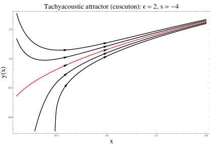
Figure 1: Evolution of the dynamical variables $x$ and $y$ in a radiation-dominated tachyacoustic model with a cuscuton Lagrangian. The Hamilton-Jacobi trajectory is the red (dashed) line.

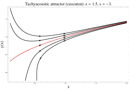
Figure 2: Evolution of the dynamical variables $x$ and $y$ in a matter-dominated tachyacoustic model with a cuscuton Lagrangian. The Hamilton-Jacobi trajectory is the red (dashed) line.

III.2 The DBI Case

Similar to the cuscuton case considered in the previous section, we can construct a Dirac-Born-Infeld Lagrangian by choosing ${\tilde{s}}=s$, so that $n=3$ in Eq. (27), which corresponds to the Lagrangian Bessada:2009ns

$${\mathcal{L}}\left(X,\phi\right)=-f^{-1}\left(\phi\right)\sqrt{1-f\left(\phi\right)X}+f^{-1}\left(\phi\right)-V\left(\phi\right).$$ (55)

For $\epsilon$ and $s$ constant we obtain an exactly solvable system, with

$$V\left(\phi\right)=3M_{P}^{2}H_{0}^{2}\left(\frac{\phi}{\phi_{0}}\right)^{-4\epsilon/s}\left[1-\left(\frac{2\epsilon}{3}\right)\frac{1}{1+\left(\phi/\phi_{0}\right)^{2}}\right],$$ (56)

and

$$f\left(\phi\right)=\left(\frac{1}{2M_{p}^{2}H_{0}^{2}\epsilon}\right)\left(\frac{\phi}{\phi_{0}}\right)^{4\epsilon/s-2}\left[1-\left(\frac{\phi}{\phi_{0}}\right)^{4}\right].$$ (57)

The sound speed (3) for the DBI Lagrangian is

$$c_{S}=\frac{1}{{\mathcal{L}}_{X}}=\sqrt{1-f\left(\phi\right)\dot{\phi}^{2}},$$ (58)

and the Hubble parameter (5) is

$$H^{2} = \frac{1}{3M_{p}^{2}}\left(2X{\mathcal{L}}_{X}-{\mathcal{L}}\right)$$ (59)

$$= \frac{1}{3M_{p}^{2}}\left[\frac{1-c_{S}}{c_{S}f\left(\phi\right)}+V\left(\phi\right)\right].$$ (60)

The equation of motion for for the field $\phi$ is then

$${\ddot{\phi}}+3Hc_{S}^{2}{\dot{\phi}}+\frac{3f^{\prime}\left(\phi\right)}{2f\left(\phi\right)}{\dot{\phi}}^{2}-\frac{f^{\prime}\left(\phi\right)}{f\left(\phi\right)^{2}}+c_{S}^{3}\left[\frac{f^{\prime}\left(\phi\right)}{f\left(\phi\right)^{2}}+V^{\prime}\left(\phi\right)\right]=0,$$ (61)

with solution

$$\dot{\phi}=-\frac{s}{2}H_{0}\phi_{0}\left(\frac{\phi}{\phi_{0}}\right)^{-2\epsilon/s+1},$$ (62)

$$H\left(\phi\right)=H_{0}\left(\frac{\phi}{\phi_{0}}\right)^{-2\epsilon/s},$$ (63)

$$c_{S}\left(\phi\right)=\left(\frac{\phi}{\phi_{0}}\right)^{2}.$$ (64)

This solution again corresponds to power-law evolution $a\propto e^{-N}\propto t^{1/\epsilon}$. As in the cuscuton case, the spectral index of scalar perturbations is

$$n=1-\frac{2\epsilon+s}{1-\epsilon-s},$$ (65)

so that the scale-invariant limit corresponds to $s=-2\epsilon$.

We study the attractor properties of this solution by defining dimensionless variables

$$x\equiv\frac{\phi}{\phi_{0}},$$ (66)

$$y\equiv\frac{\dot{\phi}}{\sqrt{3}H_{0}M_{p}},$$ (67)

and

$$v(x)\equiv\frac{V\left(\phi\right)}{3M_{p}^{2}H_{0}^{2}}=x^{-4\epsilon/s}\left[1-\left(\frac{2\epsilon}{3}\right)\frac{1}{1+x^{2}}\right],$$ (68)

$$g(x)\equiv 3M_{P}^{2}H_{0}^{2}f\left(\phi\right)=\left(\frac{3}{2\epsilon}\right)x^{4\epsilon/s-2}\left(1-x^{4}\right).$$ (69)

The dimensionless Hubble parameter is

$$h\left(x\right)\equiv\frac{H\phi_{0}}{\sqrt{3}M_{P}H_{0}}=\sqrt{\left(\frac{8\epsilon}{3s^{2}}\right)\left[\frac{1-c_{S}\left(x\right)}{c_{S}\left(x\right)g\left(x\right)}+v\left(x\right)\right]},$$ (70)

where the sound speed is

$$c_{S}^{2}=1-g\left(x\right)y^{2}\left(x\right).$$ (71)

In terms of these dimensionless variables, DBI equation of motion is:

$$y\left(x\right)y^{\prime}\left(x\right)+3hc_{S}^{2}y\left(x\right)+\frac{3}{2}\frac{g^{\prime}}{g}y^{2}\left(x\right)+(c_{S}^{3}-1)\frac{g^{\prime}}{g^{2}}+c_{S}^{3}v^{\prime}=0.$$ (72)

The analytic solution (64) is

$$y\left(x\right)=\frac{s}{2}\sqrt{\frac{8\epsilon}{3s^{2}}}x^{1-2\epsilon/s},$$ (73)

$$h\left(x\right)=\sqrt{\frac{8\epsilon}{3s^{2}}}x^{-2\epsilon/s},$$ (74)

$$c_{S}=x^{2}.$$ (75)

We evaluate the attractor behavior of this solution in the scale-invariant limit $s=-2\epsilon$. Figure (3) shows the radiation-dominated case ($\epsilon=2$), and Figure (4) shows the matter-dominated case ($\epsilon=3/2$). In both cases, the analytic solution (64) is a dynamical attractor.

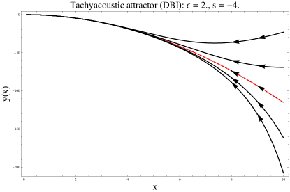
Figure 3: Evolution of the dynamical variables $x$ and $y$ in a radiation-dominated tachyacoustic model with a DBI Lagrangian. The Hamilton-Jacobi trajectory is the red (dashed) line.

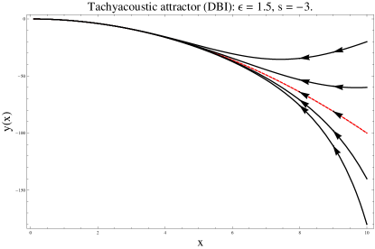
Figure 4: Evolution of the dynamical variables $x$ and $y$ in a matter-dominated tachyacoustic model with a DBI Lagrangian. The Hamilton-Jacobi trajectory is the red (dashed) line.

IV Conclusions

In this paper, we consider the dynamical stability of “tachyacoustic” cosmological models Bessada:2009ns , which generate superhorizon cosmological perturbations via a decreasing, superluminal sound speed instead of accelerating expansion (as in the case of inflation). It is known that such cosmologies can produce nearly scale-invariant scalar perturbations, consistent with current data. However, it has not been previously shown that such solutions also correspond to dynamical attractors, which is a necessary condition for such models to be cosmologically viable. Such models are realized in scalar field theory via a non-canonical Lagrangian noncanonical . In our analysis, we have considered two particular choices of Lagrangian which give rise to power-law evolution for the scale factor and sound speed, resulting in a scale-invariant primordial power spectrum. The first case is a so-called “cuscuton” Lagrangian, which is linear in the field kinetic term instead of quadratic as in the case of a canonical Lagrangian. We numerically integrate the full phase space for the field evolution, and show that the power-law tachyacoustic solution is in fact a dynamical attractor. Such models are of particular interest because they predict a detectable contribution to cosmological non-Gaussianity nongaussian . Second, we consider a Dirac-Born-Infeld (DBI) Lagrangian giving identical power-law behavior and show that the power-law solution to this Lagrangian is also a dynamical attractor in the full phase space. We present results for the scale-invariant limit, but considering a slightly “red” spectrum as favored by data does not alter the attractor properties of the solution. We conclude that, like inflation, tachyacoustic cosmology can generate a scale-invariant power spectrum via dynamically stable cosmological evolution. We note that in this analysis we consider only the classical stability of tachyacoustic models. This may not apply at the quantum level. Negative-tension branes, for example, are known to have instabilities at the quantum level Nunes:2005up ; Marolf:2001ne . However, we are not aware of any general argument indicating that theories with a superluminal sound speed are necessarily unstable to quantum mechanical flucutations.

- (1) A. H. Guth, Phys. Rev. D 23, 347 (1981). A. D. Linde, Phys. Lett. B 108, 389 (1982). A. Albrecht and P. J. Steinhardt, Phys. Rev. Lett. 48, 1220 (1982).
- (2) G. Veneziano, Phys. Lett. B 265, 287 (1991); M. Gasperini and G. Veneziano, Astropart. Phys. 1, 317 (1993) [arXiv:hep-th/9211021]; M. Gasperini and G. Veneziano, Phys. Rept. 373, 1 (2003) [arXiv:hep-th/0207130]. V. Bozza, M. Gasperini, M. Giovannini and G. Veneziano, Phys. Lett. B 543, 14 (2002) [arXiv:hep-ph/0206131]; V. Bozza and G. Veneziano, JCAP 0509, 007 (2005) [arXiv:gr-qc/0506040].
- (3) J. Khoury, B. A. Ovrut, P. J. Steinhardt and N. Turok, Phys. Rev. D 64, 123522 (2001) [arXiv:hep-th/0103239]; P. Steinhardt and N. Turok, Science 296: 1436-1439, 2002. J. L. Lehners, P. McFadden, N. Turok and P. J. Steinhardt, Phys. Rev. D 76, 103501 (2007) [arXiv:hep-th/0702153]; E. I. Buchbinder, J. Khoury and B. A. Ovrut, Phys. Rev. D 76, 123503(2007) [arXiv:hep-th/0702154]; P. Creminelli and L. Senatore, JCAP 0711, 010 (2007) [arXiv:hep-th/0702165]; K. Koyama and D. Wands, JCAP 0704, 008 (2007) [arXiv:hep-th/0703040]; K. Koyama, S. Mizuno and D. Wands, Class. Quant. Grav. 24, 3919 (2007) [arXiv:0704.1152 [hep-th]].
- (4) J. Acacio de Barros, N. Pinto-Neto, and M. A. Sagioro-Leal, Phys. Lett. A 241, 229 (1998). R. Colistete Jr., J. C. Fabris, and N. Pinto-Neto, Phys. Rev. D62, 083507 (2000). F.G. Alvarenga, J.C. Fabris, N.A. Lemos and G.A. Monerat, Gen.Rel.Grav. 34, 651 (2002).
- (5) C. Armendariz-Picon, T. Damour and V. F. Mukhanov, Phys. Lett. B 458, 209 (1999) [arXiv:hep-th/9904075]. C. Armendariz-Picon, JCAP 0610, 010 (2006) [arXiv:astro-ph/0606168]. Y. S. Piao, Phys. Rev. D 75, 063517 (2007) [arXiv:gr-qc/0609071]. J. Magueijo, Phys. Rev. Lett. 100, 231302 (2008) [arXiv:0803.0859 [astro-ph]]. J. Magueijo, Phys. Rev. D 79, 043525 (2009) [arXiv:0807.1689 [gr-qc]]. Y. S. Piao, arXiv:0807.3226 [gr-qc]. Y. -S. Piao, Phys. Lett. B 606, 245 (2005) [hep-th/0404002]. Y. -S. Piao, arXiv:1112.3737 [hep-th].
- (6) G. Geshnizjani, W. H. Kinney and A. M. Dizgah, JCAP 1111, 049 (2011) [arXiv:1107.1241 [astro-ph.CO]].
- (7) D. Bessada, W. H. Kinney, D. Stojkovic and J. Wang, arXiv:0908.3898 [astro-ph.CO].
- (8) W. H. Kinney, Phys. Rev. D 66, 083508 (2002) [arXiv:astro-ph/0206032].
- (9) R. Bean, D. J. H. Chung and G. Geshnizjani, Phys. Rev. D 78, 023517 (2008) [arXiv:0801.0742 [astro-ph]].
- (10) G. Geshnizjani, W. H. Kinney and A. M. Dizgah, JCAP 1202, 015 (2012) [arXiv:1110.4640 [astro-ph.CO]].
- (11) W. H. Kinney and K. Tzirakis, Phys. Rev. D 77, 103517 (2008) [arXiv:0712.2043 [astro-ph]].
- (12) N. Afshordi, D. J. H. Chung and G. Geshnizjani, Phys. Rev. D 75, 083513 (2007) [hep-th/0609150].
- (13) E. Silverstein and D. Tong, Phys. Rev. D 70, 103505 (2004) [arXiv:hep-th/0310221].
- (14) M. Alishahiha, E. Silverstein and D. Tong, Phys. Rev. D 70, 123505 (2004) [hep-th/0404084].
- (15) D. Bessada, JCAP 1209, 018 (2012) [arXiv:1206.0728 [gr-qc]].
- (16) J. Magueijo, J. Noller and F. Piazza, Phys. Rev. D 82, 043521 (2010) [arXiv:1006.3216 [astro-ph.CO]].
- (17) J. Noller and J. Magueijo, Phys. Rev. D 83, 103511 (2011) [arXiv:1102.0275 [astro-ph.CO]].
- (18) D. Seery and J. E. Lidsey, JCAP 0506, 003 (2005) [astro-ph/0503692].
- (19) X. Chen, M. -x. Huang, S. Kachru and G. Shiu, JCAP 0701, 002 (2007) [hep-th/0605045].
- (20) E. Komatsu et al. [WMAP Collaboration], Astrophys. J. Suppl. 180, 330 (2009) [arXiv:0803.0547 [astro-ph]].
- (21) V. Mukhanov, “Physical Foundations of Cosmology”, Cambridge University Press, Cambridge, UK (2005).
- (22) N. J. Nunes and M. Peloso, Phys. Lett. B 623, 147 (2005) [hep-th/0506039].
- (23) D. Marolf and M. Trodden, Phys. Rev. D 64, 065019 (2001) [hep-th/0102135].