Interpolation Theorems in Harmonic Analysis

This thesis is “dedicated” to the first Rutgers-NYU segway polo champion: come forth and claim your prize!

Preface

The present thesis contains an exposition of interpolation theory in harmonic analysis, focusing on the complex method of interpolation. Broadly speaking, an interpolation theorem allows us to guess the “intermediate” estimates between two closely-related inequalities. To give an elementary example, we take a square-integrable function $f$ on the real line. It is a standard result from real analysis that $f$ satisfies the $L^{2}$-Hölder inequality

$$\int_{-\infty}^{\infty}\left|f(x)g(x)\right|\,dx\leq\left(\int_{-\infty}^{\infty}|f(x)|^{2}\,dx\right)^{1/2}\left(\int_{-\infty}^{\infty}|g(x)|^{2}\,dx\right)^{1/2}.$$ (1)

for every integrable function $g$ on the real line with compact support. If, in addition, $f$ satisfies the integral inequality

$$\int_{-\infty}^{\infty}|f(x)g(x)|\,dx\leq\left(\int_{-\infty}^{\infty}|f(x)|^{2}\,dx\right)^{1/2}\left(\int_{-\infty}^{\infty}|g(x)|\,dx\right)$$ (2)

for all such $g$, it then follows “from interpolation” that the inequality

$$\int_{-\infty}^{\infty}|f(x)g(x)|\,dx\leq\left(\int_{-\infty}^{\infty}|f(x)|^{2}\,dx\right)^{1/2}\left(\int_{-\infty}^{\infty}|g(x)|^{p}\,dx\right)^{1/p}$$ (3)

holds for all $1\leq p\leq 2$ and all $g$ on the real line with compact support.

From a more abstract viewpoint, we can consider interpolation as a tool that establishes the continuity of “in-between” operators from the continuity of two endpoint operators. The above example can be viewed as a study of the “multiplication by $f$” operator

$$(Tg)(x)=f(x)g(x).$$

In the language of Lebesgue spaces, inequality (1) implies that $T$ is a continuous mapping from the function space $L^{2}$ to itself, and inequality (2) implies that $T$ is a continuous mapping from $L^{2}$ to another function space $L^{1}$. The conclusion, then, is that $T$ maps $L^{2}$ continuously into the “interpolation spaces” $L^{p}$ ($1\leq p\leq 2$) as well.

Presented herein are a study of four interpolation theorems, the requisite background material, and a few applications. The materials introduced in the first three sections of Chapter 1 are used to motivate and prove the Riesz-Thorin interpolation theorem and its extension by Stein, both of which are presented in the fourth section. Chapter 2 revolves around Calderón’s complex method of interpolation and the interpolation theorem of Fefferman and Stein, with the material in between providing the necessary examples and tools. The two theorems are then applied to a brief study of linear partial differential equations, Sobolev spaces, and Fourier integral operators, presented in the last section of the second chapter.

I have approached the project mainly as an exercise in expository writing. As such, I have tried to keep a real audience in mind throughout. Specifically, my aim was to make the present thesis accessible to Rutgers graduate students who have taken Math 501, 502, and 503. This means that I have assumed familiarity with the standard material in advanced calculus, complex analysis, linear algebra and point-set topology. In addition, I expect the reader to be conversant in the language of measure and integration theory including Lebesgue spaces ($L^{p}$ spaces), and of functional analysis up to basic Banach and Hilbert space theory. Beyond those, the required tools from functional analysis are summarized in the beginning of Chapter 2, and elements of harmonic analysis are introduced throughout the thesis.

Before I realized how much time it would take to develop each topic at hand, I had planned to include some harmonic function theory, maximal function theory of Hardy and Littlewood, the interpolation theorem of Marcinkiewicz, the standard material on the theory of singular integral operators, and the Lions-Peetre method of real interpolation as a generalization of Maricnkiewicz. This never happened, and what I had in mind is reduced to a brief exposition in the further-results section of Chapter 2. Of course, given the length of the present thesis as is, I simply would not have had the time and energy to give the extra materials the care they deserve.

Nevertheless, the inclusion of the theory of singular integral operators would have helped motivating the section on Fefferman-Stein theory in Chapter 2, which I believe is extremely condensed and, frankly, dry as it stands now. Moreover, I was not able to come up with a coherent narrative for the section on the functional-analytic prerequisites in the beginning of Chapter 2. Is there any way to make a “random collection of things you should probably know before reading” section flow pleasantly smooth without expanding it into a whole chapter or a book? I do not have a good answer at the present moment.

But, enough excuses. I had a lot of fun writing this thesis, and I hope that I managed to produce an enjoyable read. Please feel free to send any comments or corrections to markhkim@dimax.rutgers.edu.

Acknowledgements

My deepest gratitude goes to my thesis advisor, Michael Beals. It is the brief conversation Professor Beals and I had on my first visit to Rutgers University that gave me the courage to pursue mathematics, the course he taught in my second-semester freshman year that convinced me to study analysis, and the numerous reading courses he gave over the following years that cultivated my current interests in the field. From the day I set my foot on campus to the very last day as an undergraduate, Professor Beals has been the greatest mentor I could possibly hope for. Indeed, it is he who taught me most of the mathematics I know, supported me wholeheartedly in my numerous academic pursuits over the years, and counseled me ever so patiently in times of trouble.

I would also like to express my gratitude to my academic advisor and the chair of the honors track, Simon Thomas. There have been more than a few times I had let myself be consumed by unrealistic, overly ambitious projects, and Professor Thomas never hesitated to provide me with a dose of reality and set me on the right path. He is also one of the best lecturers I know of, and my strong interest in mathematical exposition was, in part, cultivated in his course I took as a sophomore. I am truly fortunate to have had two amazing mentors throughout my undergraduate career.

I have benefited greatly from conversing with other professors in the department—about the project, and mathematics at large. Discussions with Eric Carlen, Roe Goodman, Robert Wilson, and Po Lam Yung have been especially helpful. The summer school in analysis and geometry at Princeton University in 2011 also contributed significantly to my understanding of the background material and their interactions with other fields. Particularly useful were the lectures by Kevin Hughes, Lillian Pierce, and Eli Stein. I would like to offer a special thanks to Professor Stein, who have written the wonderful textbooks that I have used again and again over the course of the project.

I am also grateful to Itai Feigenbaum, Matt Inverso, and Jun-Sung Suh for putting up with my endless rants and keeping me sane, and Matt D’Elia for being a fantastic study buddy. A warm thank-you goes to my “graduate officemates” Katy Craig and Glen Wilson in Hill 603, and Tim Naumotivz, Matthew Russell, and Frank Seuffert in Hill 605, who assured me that I am not the only apprentice navigator in the vast ocean of mathematics. And last but not least, a bow to my parents for keeping me alive for the past 23 years and supporting me through 17 years of formal education. Those are awfully big numbers, if you ask me.

Contents

1. ‣ Interpolation Theorems in Harmonic Analysis
2. 1 The Classical Theory of Interpolation
   1. 1.1 Elements of Integration Theory
      1. 1.1.1 Measures and Integration
      2. 1.1.2 $L^{p}$ Spaces
      3. 1.1.3 $\sigma$-Finite Measure Spaces
      4. 1.1.4 The Lebesgue Measure
   2. 1.2 Approximation in $L^{p}$ Spaces
      1. 1.2.1 Approximation by Continuous Functions
      2. 1.2.2 Convolutions
      3. 1.2.3 Approximation by Smooth Functions
   3. 1.3 The Fourier Transform
      1. 1.3.1 The $L^{1}$ Theory
      2. 1.3.2 The $L^{2}$ Theory
      3. 1.3.3 The $L^{p}$ Theory
   4. 1.4 Interpolation on $L^{p}$ Spaces
      1. 1.4.1 The Riesz-Thorin Interpolation Theorem
      2. 1.4.2 Corollaries of the Interpolation Theorem
      3. 1.4.3 The Stein Interpolation Theorem
   5. 1.5 Additional Remarks and Further Results
3. 2 The Modern Theory of Interpolation
   1. 2.1 Elements of Functional Analysis
      1. 2.1.1 Continuous Linear Functionals on Fréchet Spaces
      2. 2.1.2 Complex Analysis of Banach-valued Functions
      3. 2.1.3 Spectra of Operators on Banach Spaces
      4. 2.1.4 Compactness of the Unit Ball
      5. 2.1.5 Bounded Linear Maps between Banach Spaces
      6. 2.1.6 Spectral Theory of Self-Adjoint Operators
   2. 2.2 The Complex Interpolation Method
      1. 2.2.1 Complex Interpolation
      2. 2.2.2 Interpolation of $L^{p}$ Spaces
      3. 2.2.3 Interpolation of Hilbert Spaces
   3. 2.3 Generalized Functions
      1. 2.3.1 The Schwartz Space
      2. 2.3.2 Tempered Distributions
      3. 2.3.3 Operations on Tempered Distributions
      4. 2.3.4 Convolution Operators and Fourier Multipliers
   4. 2.4 The Hilbert Transform
      1. 2.4.1 The Distribution $\operatorname{pv}(\frac{1}{x})$ and the $L^{2}$ Theory
      2. 2.4.2 The $L^{p}$ Theory
      3. 2.4.3 Singular Integral Operators
   5. 2.5 Hardy Spaces and $\operatorname{BMO}$
      1. 2.5.1 The Hardy Space $H^{1}$
      2. 2.5.2 Interlude: The Maximal Function
      3. 2.5.3 Functions of Bounded Mean Oscillation
      4. 2.5.4 Interpolation on $H^{1}$ and $\operatorname{BMO}$
   6. 2.6 Applications to Differential Equations
      1. 2.6.1 Fundamental Solutions
      2. 2.6.2 Regularity of Solutions
      3. 2.6.3 Sobolev Spaces
      4. 2.6.4 Analysis of the Homogeneous Wave Equation
   7. 2.7 Additional Remarks and Further Results

Chapter 1 The Classical Theory of Interpolation

In the first chapter, we study two interpolation theorems, both of which are presented in §1.4. Interpolation theory began with a 1927 theorem of Marcel Riesz, first published in [Rie27b]. Riesz convexity theorem, as it is called, did not arise as a theorem of harmonic analysis, as the paper dealt with the theory of bilinear forms. It was Riesz’s student G. Olof Thorin with his thesis [Tho48] who appropriately generalized the theorem of Riesz and placed it in its proper context. The complex-analytic method used in the proof of the Riesz-Thorin interpolation theorem was then generalized by Elias M. Stein, allowing for interpolation of families of operators. This result, known as the Stein interpolation theorem, was included in his 1955 doctoral dissertation and was subsequently published in [Ste56].

The first two sections of the chapters are devoted to developing the necessary tools for stating and proving the interpolation theorems. We review the theory of measure and integration in the first section, which is included mainly as a convenient reference. In the second section, we tackle approximation theorems in Lebesgue spaces, which provide a convenient way of studying function spaces by focusing on small samples of functions. We then switch gears and present the basic theory of Fourier transform in the third section. This serves primarily to motivate the Riesz-Thorin interpolation theorem and to provide a useful example to which the theorem can be applied. The chapter culminates in the fourth and the last section, in which we state and prove the Riesz-Thorin interpolation and its generalization by Stein.

1.1 Elements of Integration Theory

We begin the chapter by collecting the necessary facts from measure and integration theory. The present section is meant to serve only as a quick reference, and so the details will necessarily be sparse. See [SS11], [SS05], [Fol99], [Rud86], or any other standard textbook on the subject for a more detailed treatment.

1.1.1 Measures and Integration

Recall that a $\sigma$-algebra on a nonempty set $X$ is a collection $\mathfrak{M}$ of subsets of $X$ such that

1. $\varnothing\in\mathfrak{M}$ and $X\in\mathfrak{M}$.

2. If $(E_{n})_{n=1}^{\infty}$ is a sequence in $\mathfrak{M}$, then $\bigcup_{n}E_{n}\in\mathfrak{M}$.

3. If $E\in\mathfrak{M}$, then $X\smallsetminus E\in\mathfrak{M}$.

Note that (b) and (c) imply

1. If $(E_{n})_{n=1}^{\infty}$ is a sequence in $\mathfrak{M}$, then $\bigcap_{n}E_{n}\in\mathfrak{M}$.

The pair $(X,\mathfrak{M})$ is referred to as a measurable space. Given a measurable space $(X,\mathfrak{M})$, we say that a subset of $X$ is measurable if it is an element of $\mathfrak{M}$. A measure on $(X,\mathfrak{M})$ is a function $\mu:\mathfrak{M}\to[0,\infty]$ that is countably additive, viz.,

$$\mu\left(\bigcup_{n=1}^{\infty}E_{n}\right)=\sum_{n=1}^{\infty}\mu(E_{n})$$

for every pairwise disjoint sequence $(E_{n})_{n=1}^{\infty}$ of measurable sets. Every measure $\mu$ on $X$ satisfies the following properties:

1. $\mu(\varnothing)=0$;

2. Monotonicity. If $E$ and $F$ are measurable subsets of $X$ and if $E\subseteq F$, then $\mu(E)\leq\mu(F)$.

3. Countable subadditivity. If $(E_{n})_{n=1}^{\infty}$ is a sequence of measurable subsets of $X$, then

   $$\mu\left(\bigcup_{n=1}^{\infty}E_{n}\right)\leq\sum_{n=1}^{\infty}\mu(E_{n}).$$

4. Continuity from below. If $E_{1}\subseteq E_{2}\subseteq E_{3}\subseteq\cdots$ is a sequence of measurable subsets of $X$, then

   $$\mu\left(\bigcup_{n=1}^{\infty}E_{n}\right)=\lim_{n\to\infty}\mu(E_{n}).$$

5. Continuity from above. If $E_{1}\supseteq E_{2}\supseteq E_{3}\cdots$ is a sequence of measurable subsets of $X$ such that $\mu(E_{1})<\infty$, then

   $$\mu\left(\bigcap_{n=1}^{\infty}E_{n}\right)=\lim_{n\to\infty}\mu(E_{n}).$$

Given a nonempty set $X$, a $\sigma$-algebra $\mathfrak{M}$ on $X$, and a measure $\mu$ on the measurable space $(X,\mathfrak{M})$, we refer to triple $(X,\mathfrak{M},\mu)$ as a measure space. A measure space $(X,\mathfrak{M},\mu)$ is said to be finite if $\mu(X)<\infty$, $\sigma$-finite if there exists a sequence $(E_{n})_{n=1}^{\infty}$ of finite-measure sets whose union is $X$, and complete if all subsets of measure-zero sets are measurable. We often talk about a finite measure, a $\sigma$-finite measure, or a complete measure: this usage introduces no ambiguity, as specifying a measure picks out a unique $\sigma$-algebra as its domain, and this $\sigma$-algebra, in turn, determines a unique base set. Similarly, we usually speak of measures on the base set $X$, even though the measures are, strictly speaking, defined on measurable spaces.

If $X$ is a topological space, then we define the Borel $\sigma$-algebra to be the smallest $\sigma$-algebra on $X$ containing all open subsets of $X$. A Borel set in $X$ is an element of the Borel $\sigma$-algebra on $X$, and a Borel measure on $X$ is a measure on $X$ that renders all Borel sets measurable. The canonical measure on $\mathbb{R}^{d}$, the $d$-dimensional Lebesgue measure, is the unique complete translation-invariant Borel measure $\mathscr{L}^{d}$ on $\mathbb{R}^{d}$ with the normalization $\mathscr{L}^{d}([0,1]^{d})=1$. If there is no danger of confusion, $m(E)$ or $|E|$ is often used in place of $\mathscr{L}^{d}(E)$. We shall have more to say about the Lebesgue measure later in this section. For now, we merely remark that the Lebesgue measure is $\sigma$-finite.

Given a measure space $(X,\mathfrak{M},\mu)$ and a topological space $Y$, we say that a function $f:X\to Y$ is measurable if each open set $E$ in $Y$ has a measurable preimage $f^{-1}(E)$. If $X$ is a topological space and $\mu$ a Borel measure, then the definition renders all continuous functions measurable. If $Y$ is $\mathbb{R}$ or $\mathbb{C}$, then the sums and products of measurable functions are measurable. We observe that the supremum, the infimum, the limit superior, and the limit inferior of a sequence of measurable functions is measurable. This, in particular, implies that the limit of a pointwise convergent sequence of measurable functions is measurable. In fact, if the set of divergence is of measure zero, then this continues to hold. In other worlds, the limit of a pointwise almost-everywhere convergent sequence of measurable functions is measurable. We say that a property $P$ holds almost everywhere if the set on which $P$ does not hold is of measure zero.

Let $(X,\mathfrak{M},\mu)$ be a measure space. The characteristic function, or the indicator function, of $E\subseteq X$ is defined to be

$$\chi_{E}(x)=\begin{cases}1&\mbox{ if }x\in E;\\ 0&\mbox{ if }x\in X\smallsetminus E.\end{cases}$$

A simple function $s$ on $X$ is a finite linear combination

$$s(x)=\sum_{n=1}^{N}\lambda_{n}\chi_{E_{n}}$$

of characteristic functions, where each $\lambda_{n}$ is a complex number and $E_{n}$ a measurable set. Note that simple functions are automatically measurable. The (Lebesgue) integral is defined to be the sum

$$\int s\,d\mu=\int_{X}s(x)\,d\mu(x)=\sum_{n=1}^{N}\lambda_{n}\mu(E_{n}).$$

We extend the definition of the integral to nonnegative measurable functions $f$ on $X$ by setting

$$\int f\,d\mu=\int_{X}f(x)\,d\mu(x)=\sup\left\{\int s\,d\mu:s\mbox{ is simple and }0\leq s\leq f\right\}$$

and call $f$ integrable if the integral is finite. With this definition, we can state one of the fundamental theorems in measure theory, the monotone convergence theorem: every increasing sequence $(f_{n})_{n=1}^{\infty}$ of nonnegative integrable functions on $X$ converging pointwise almost everywhere to a function $f$ on $X$ satisfies the identity

$$\lim_{n\to\infty}\int f_{n}\,d\mu=\int\lim_{n\to\infty}f_{n}\,d\mu=\int f\,d\mu.$$

The theorem allows us to approximate the integral of nonnegative measurable functions by integrals of simple functions. Indeed, every nonnegative measurable function $f$ on $X$ admits an increasing sequence $(s_{n})_{n=1}^{\infty}$ of nonnegative simple functions that converge pointwise to $f$ and uniformly to $f$ on all subsets of $X$ on which $f$ is bounded. For non-increasing sequences of functions, we have Fatou’s lemma, which states that every sequence $(f_{n})_{n=1}^{\infty}$ of nonnegative measurable functions on $X$ satisfies the inequality

$$\int\liminf_{n\to\infty}f_{n}\,d\mu\leq\liminf_{n\to\infty}\int f_{n}\,d\mu.$$

Before we extend the definition of the integral to general cases, we take a moment to tackle a minor technical issue. Functions like $f(x)=x^{-1/2}\chi_{[0,1]}$ are “integrable over $\mathbb{R}$” and have finite integrals, but they are not functions on $\mathbb{R}$ in the traditional sense, for $x=0$ must be excluded from the domain. In order to incorporate such functions into the framework of Lebesgue integration, we ought to turn them into measurable functions on their natural “domain space”. The solution is to consider the extended number system $\bar{\mathbb{R}}$, which consists of the real numbers, the negative infinity $-\infty$, and the positive infinity $\infty$. We define the arithmetic operations on $\bar{\mathbb{R}}$ by inheriting the operations from $\mathbb{R}$ and then by setting

$$x\pm\infty=\pm\infty,\hskip 7.22743pt\frac{x}{\pm\infty}=0,\hskip 7.22743pty\cdot(\pm\infty)=\pm\infty,\hskip 7.22743pt(-y)\cdot(\pm\infty)=\mp\infty$$

for all $x\in\mathbb{R}$ and $y\in\mathbb{R}\smallsetminus\{0\}$; we do not attempt to define $\infty-\infty$. In measure theory, we typically set

$$0\cdot\pm\infty=0,$$

so that the values of an extended real-valued function on a set of measure zero are negligible. We say that a function $f:X\to\bar{\mathbb{R}}$ is measurable if $f^{-1}([-\infty,a))$ is measurable in $X$ for each $a\in\mathbb{R}$. With the standard topology on $\bar{\mathbb{R}}$, this definition agrees with the standard definition of measurable functions given above: see §§1.5.1 for a discussion.

We now fix an arbitrary measurable extended real-valued function $f$ on $X$ and define

$$f^{+}(x)=\max\{f(x),0\}\hskip 14.45377pt\mbox{and}\hskip 14.45377ptf^{-}(x)=\max\{-f(x),0\}.$$

$f^{+}$ and $f^{-}$ are nonnegative, measurable, extended real-valued functions, and so we can define the integrals $\int f^{+}$ and $\int f^{-}$ by a simple modification of the definition of integral for nonnegative real-valued functions. Since $f$ can be written as the difference $f^{+}-f^{-}$, it is natural to define the integral of $f$ to be

$$\int f\,d\mu=\int_{X}f(x)\,d\mu(x)=\int f^{+}\,d\mu-\int f^{-}\,d\mu,$$

provided that the difference is well-defined. We say that $f$ is integrable if and only if the integral of $f$ is finite.

If $f$ is complex-valued, we use the decomposition

$$f=\operatorname{Re}f^{+}-\operatorname{Re}f^{-}+i(\operatorname{Im}f^{+}-\operatorname{Im}f^{-})$$

to define the integral of $f$ to be

$$\int_{X}f(x)\,d\mu(x)=\int\operatorname{Re}f^{+}\,d\mu-\int\operatorname{Re}f^{-}\,d\mu+i\left(\int\operatorname{Im}f^{+}\,d\mu-\int\operatorname{Im}f^{-}\,d\mu\right),$$

where

$$\operatorname{Re}f^{+}(x) = \max\{\operatorname{Re}f(x),0\};$$

$$\operatorname{Re}f^{-}(x) = \max\{-\operatorname{Re}f(x),0\};$$

$$\operatorname{Im}f^{+}(x) = \max\{\operatorname{Im}f(x),0\};$$

$$\operatorname{Im}f^{-}(x) = \max\{-\operatorname{Im}f(x),0\}.$$

Again, the integral of $f$ is defined only when the above sum of integrals is well-defined, and we say that $f$ is integrable if the integral of $f$ is finite. The main convergence theorem for this definition is the dominated convergence theorem: a sequence $(f_{n})_{n=1}^{\infty}$ of measurable functions converging pointwise almost everywhere to $f$ and satisfying the bound $|f_{n}|\leq g$ almost everywhere with an integrable function $g$ satisfies the following identity:

$$\lim_{n\to\infty}\int f_{n}\,d\mu=\int\lim_{n\to\infty}f_{n}\,d\mu=\int f\,d\mu.$$

Instrumental in proving the aforementioned convergence theorems are the following basic properties of the integral:

1. $\int(f+g)\,d\mu=\int f\,d\mu+\int g\,d\mu$.

2. $\int(\lambda f)\,d\mu=\lambda\int f\,d\mu$ for each complex number $\lambda$.

3. If $f\leq g$, then $\int f\,d\mu\leq\int g\,d\mu$.

4. $|\int f\,d\mu|\leq\int|f|\,d\mu$.

5. If $f=0$ almost everywhere, then $\int f\chi_{E}\,d\mu=0$ for all $E$.

6. If $\mu(E)=0$, then $\int f\chi_{E}\,d\mu=0$ for all $f$.

(a) and (b) imply that the integral is a linear functional on the Lebesgue space $L^{p}(X,\mu)$, which we shall define in due course. (e) and (f) can be rephrased in terms of integrating over subsets: if $f$ is a complex-valued measurable function on $X$ and $E$ a measurable subset of $X$, then the integral of $f$ over $E$ is

$$\int_{E}f\,d\mu=\int_{X}f\chi_{E}\,d\mu.$$

(d) implies that the integrability of $|f|$ establishes the integrability of $f$. In fact, a simple computation shows that the converse is true as well.

1.1.2 $L^{p}$ Spaces

In light of the above observation, we see that the collection $L^{1}(X,\mu)$ of complex-valued measurable functions $f$ on $X$ such that $\int|f|\,d\mu<\infty$ collects all integrable complex-valued functions on $X$. We thus define the $L^{1}$-norm $\|f\|_{1}$ of $f\in L^{1}(X,\mu)$ to be the integral $\int|f|\,d\mu$. Note that the $L^{1}$-norm is not a norm as it is, since functions that are zero almost everywhere still have the $L^{1}$-norm of zero. To rectify this issue, we consider $L^{1}(X,\mu)$ to be the quotient vector space defined by the equivalence relation

$$f\sim g\Leftrightarrow f=g\mbox{ almost everywhere},$$

at which point the $L^{1}$ norm becomes a bona fide norm on $L^{1}(X,\mu)$.

We pause to make two remarks. Note first that every integrable function must be finite almost everywhere, whence each extended real-valued integrable function is equal almost-everywhere to a complex-valued integrable function. Therefore, extended real-valued integrable functions can be put in $L^{1}(X,\mu)$ without disrupting the complex-vector-space structure thereof. We also point out that the equivalence-class definition provides no real benefit beyond resolving a few technical issues. Therefore, we shall be intentionally sloppy and speak of functions in $L^{1}(X,\mu)$, unless structural nit-picking is necessary.

Endowing $L^{1}(X,\mu)$ with the corresponding norm topology, we can now consider the dominated convergence theorem as a sufficient condition for turning pointwise almost-everywhere convergence of integrable functions into convergence in the $L^{1}$-norm. We also have a partial converse, which states that every sequence of integrable functions converging in the $L^{1}$-norm admits a subsequence, with a dominating function in $L^{1}$, that converges pointwise almost everywhere. We note that the $L^{1}$-metric

$$d_{L^{1}}(f,g)=\|f-g\|_{1}$$

is complete, so that $L^{1}(X,\mu)$ is a Banach space, a normed linear space whose norm-induced metric topology is complete.

It is also useful to consider the space $L^{2}(X,\mu)$ of square-integrable functions on $X$, with the quotient-space construction as above to avoid technical problems. The bilinear form

$$\langle f,g\rangle_{2}=\int_{X}f\bar{g}\,d\mu$$

is an inner product on $L^{2}(X,\mu)$, which is well-defined by the Cauchy-Schwarz inequality:

$$|\langle f,g\rangle_{2}|\leq\|f\|_{2}\|g\|_{2}.$$

Here $\|\cdot\|_{2}$ is the corresponding $L^{2}$-norm

$$\|f\|_{2}=\langle f,f\rangle_{2}^{1/2}=\left(\int_{X}|f|^{2}\,d\mu\right)^{1/2},$$

which furnishes a complete metric. Therefore, $L^{2}(X,\mu)$ is a Hilbert space, an inner product space whose norm-induced metric topology is complete. Even better, if we set $X$ to be the Euclidean space $\mathbb{R}^{d}$ and $\mu$ the $d$-dimensional Lebesgue measure, then the corresponding $L^{2}$-space is separable, viz., it contains a countable dense subset. Since all separable Hilbert spaces are unitarily isomorphic to one another, $L^{2}$ is, in a sense, the Hilbert space.

Recall that a linear functional on a real or complex vector space $V$ is a linear transformation on $V$ into the scalar field $\mathbb{F}$, which is taken to be either $\mathbb{R}$ or $\mathbb{C}$. If $V$ is a normed linear space, a linear functional $l$ on $V$ is bounded in case it admits a constant $k$ such that

$$|lv|\leq k\|v\|_{V}$$ (1.1)

for all $v\in V$. We note that $l$ is bounded if and only if $l$ is continuous with respect to the norm topology of $V$. The collection $V^{*}$ of bounded linear functionals on $V$ forms a vector space, called the dual space of $V$. It is a standard result in real analysis that $V^{*}$ is a Banach space with the operator norm

$$\|l\|_{V^{*}}=\sup_{\|v\|\leq 1}|lv|,$$

which, in turn, is the infimum of all possible $k$ in (1.1).

Since many transformations of functions that arise in mathematical analysis can be understood as bounded linear functionals on function spaces, it is of interest to describe them as concretely as possible. A common approach, known as a representation theorem, is to determine the obvious bounded linear functionals on the given function space, and then to investigate the extent in which arbitrary bounded linear functionals can be represented by the obvious ones. For $L^{2}$, we have a wonderfully concrete representation theorem, due to Frigyes Riesz:

Theorem 1.1 (F. Riesz representation theorem, Hilbert-space version).

If $\mathcal{H}$ is a Hilbert space, then each bounded linear functional $l:\mathcal{H}\to\mathbb{C}$ admits a unique element $u\in\mathcal{H}$ such that

$$lv=\langle v,u\rangle_{\mathcal{H}}$$

for all $v\in\mathcal{H}$. Moreover, $\|l\|_{\mathcal{H}^{*}}=\|u\|_{\mathcal{H}}$.

It follows that we can identify each element of $\mathcal{H}^{*}$ with an element of $\mathcal{H}$. In particular, we conclude that

$$(L^{2}(X,\mu))^{*}=L^{2}(X,\mu)$$

in light of the above identification.

Having considered $L^{1}$ and $L^{2}$, we now define, for each $p\in[1,\infty)$, the Lebesgue space $L^{p}(X,\mu)$ of order $p$ on $X$ by collecting the complex-valued measurable functions $f$ on $X$ such that

$$\|f\|_{p}=\left(\int_{X}|f|^{p}\,d\mu\right)^{1/p}<\infty.$$

The standard quotient construction is applied here as well, turning $\|\cdot\|_{p}$ into a norm. With the language of Lebesgue spaces, Hölder’s inequality can be stated succinctly as

$$\|fg\|_{1}\leq\|f\|_{p}\|g\|_{p^{\prime}},$$

where $p>1$ and $p^{\prime}$ is the conjugate exponent

$$p^{\prime}=\frac{p}{p-1}$$

of $p$. Note that $1/p+1/p^{\prime}=1$.

Note that if $f\in L^{1}(X,\mu)$ and $g$ is bounded, then

$$\|fg\|_{1}\leq\|f\|_{1}\sup_{x\in X}|g(x)|.$$

Expanding on this idea, we introduce the space $L^{\infty}(X,\mu)$ of complex-valued measurable functions $f$ on $X$ whose essential supremum

$$\|f\|_{\infty}=\inf\{\lambda\in\mathbb{R}:\mu(\{x:|f(x)|>\lambda\})=0\}$$

is finite. The space $L^{\infty}(X,\mu)$ can be considered as a “limiting space” of $L^{p}(X,\mu)$, for if $f\in L^{\infty}$ is supported on a set of finite measure, then $f\in L^{p}$ for all $p<\infty$ and

$$\lim_{p\to\infty}\|f\|_{p}=\|f\|_{\infty}.$$

We remark that Hölder’s inequality holds for $p=1$ as well, with the identification $1/\infty=0$ to yield $p^{\prime}=\infty$.

Given $p\in[1,\infty]$, Minkowski’s inequality establishes the triangle inequality for $\|\cdot\|_{p}$, thus turning $\|\cdot\|_{p}$ into a norm on $L^{p}(X,\mu)$. Moreover, the Riesz-Fischer theorem guarantees that $L^{p}(X,\mu)$ is a Banach space. A partial converse to the $L^{p}$ dominated convergence theorem continues to hold, so that a sequence of functions converging in the $L^{p}$ norm admits a pointwise almost-everywhere convergent subsequence with a dominating function in $L^{p}$, continues to hold.

Observe, however, that the dominated convergence theorem fails to hold on $L^{\infty}$. The $L^{p}$ representation theorem for $L^{p}$, which yields the identification $(L^{p})^{*}=L^{p^{\prime}}$, also fails to hold for $p=\infty$: see §§1.5.2. We shall have more to say about the representation theorem in the next subsection.

1.1.3 $\sigma$-Finite Measure Spaces

In this subsection, we review three major theorems of measure and integration theory that requires the $\sigma$-finiteness hypothesis. The first is the $L^{p}$ representation theorem, as was alluded to above:

Theorem 1.2 (F. Riesz representation theorem, $L^{p}$-space version).

Suppose that $(X,\mathfrak{M},\mu)$ is a $\sigma$-finite measure space. If $p\in[1,\infty)$, then each bounded linear functional $l$ on $L^{p}(X,\mu)$ admits a unique linear function $u\in L^{p^{\prime}}(X,\mu)$ such that

$$l(f)=\int fu\,d\mu$$ (1.2)

for all $f\in L^{p}(X,\mu)$. Moreover, $\|l\|_{(L^{p})^{*}}=\|u\|_{L^{q^{\prime}}}$, whence $(L^{p})^{*}$ is isometrically isomorphic to $L^{p^{\prime}}$.

It is an easy consequence of Hölder’s inequality that every function of the form (1.2) is a bounded linear functional on $L^{p}$. The representation theorem states that linear functionals of the form (1.2) are, in fact, all bounded linear functionals on $L^{p}$.

Since the proof of the representation theorem makes use of a few key notions that we shall need in later sections, we study it in detail. To this end, we fix a measurable space $(X,\mathfrak{M})$ and recall that a function $\nu:\mathfrak{M}\to\mathbb{C}$ is a complex measure if, for each $E\in\mathfrak{M}$ and every countable partition $\{E_{n}:n\in\mathbb{N}\}$ of $E$ in $\mathfrak{M}$, the function $\nu$ is countably additive, viz.,

$$\nu(E)=\sum_{n=1}^{\infty}\nu(E_{n}).$$

Note that the definition forces $\mu(X)<\infty$.

We sometimes use the name positive measures for measures proper in order to distinguish them from complex measures. In fact, there is a canonical way of assigning a positive measure corresponding to each complex measure $\nu$: the total variation of $\nu$ is the positive measure $|\nu|$ defined to be

$$|\nu|(E)=\sup_{E\in\mathfrak{M}}\sum_{n=1}^{\infty}|\nu(E_{n})|$$

for each $E\in\mathfrak{M}$, where the supremum is taken over all partitions $\{E_{n}:n\in\mathbb{N}\}$ of $E$ belonging to $\mathfrak{M}$. Recalling that a measure $\nu$, complex or positive, on $(X,\mathfrak{M})$ is said to be absolutely continuous with respect to a positive measure $\mu$ on $(X,\mathfrak{M})$ if $\nu(E)=0$ for all $E\in\mathfrak{M}$ such that $\mu(E)=0$, we see that $\nu$ is absolutely continuous with respect to $|\nu|$. In general, we write

$$\nu\ll\mu$$

to denote the absolute continuity of $\nu$ with respect to $\mu$.

A polar opposite notion to absolute continuity is defined as follows: two measures $\nu_{1}$ and $\nu_{2}$, positive or complex, are said to be mutually singular if there exists a disjoint pair of measurable sets $A$ and $B$ such that

$$\nu_{1}(E)=\nu_{1}(A\cap E)\hskip 14.45377pt\mbox{and}\hskip 14.45377pt\nu_{2}(E)=\nu_{2}(B\cap E)$$

for all $E\in\mathfrak{M}$. We write

$$\nu_{1}\perp\nu_{2}$$

to denote the mutual singularity of $\nu_{1}$ and $\nu_{2}$.

We are now ready to state the second theorem of this section, which is the main ingredient of the proof of the representation theorem.

Theorem 1.3 (Lebesgue-Radon-Nikodym).

Let $(X,\mathfrak{M})$ be a measurable space, $\nu$ a complex measure, and $\mu$ a positive $\sigma$-finite measure. Then there is a unique pair of complex measures $\nu_{a}$ and $\nu_{s}$ such that

$$\nu=\nu_{a}+\nu_{s},\hskip 7.22743pt\nu_{a}\ll\mu,\hskip 7.22743pt\nu_{s}\perp\mu,$$

and there exists a $u\in L^{1}(X,\mu)$ such that

$$\nu_{a}(E)=\int_{E}u\,d\mu$$

for all $E\in\mathfrak{M}$. Any such function agrees with $u$ almost everywhere on $X$.

Two remarks are in order. First, if $\nu$ is a positive finite measure, then so are $\nu_{a}$ and $\nu_{s}$. Second, if $\nu\ll\mu$, then $d\nu=ud\mu$ for an $L^{1}$ function $u$ defined uniquely almost everywhere. This $u$ is called the Radon-Nikodym derivative and is denoted by $\frac{d\nu}{d\mu}$, so that

$$d\nu=\frac{d\nu}{d\mu}d\mu.$$

Having stated the Lebesgue-Radon-Nikodym theorem, we proceed to the proof of the $L^{p}$ representation theorem. In what follows, we use the complex signum function

$$\operatorname{sgn}z=\begin{cases}\frac{z}{|z|}&\mbox{ if }z\in\mathbb{C}\smallsetminus\{0\};\\ 0&\mbox{ if }z=0.\end{cases}$$

Proof of Theorem 1.2.

We first claim that the norm of $u\in L^{p^{\prime}}(X,\mu)$ can be computed by the identity

$$\|u\|_{p^{\prime}}=\sup_{\|f\|_{p}\leq 1}\left|\int fu\,d\mu\right|.$$ (1.3)

Note first that

$$\int|fu|\,d\mu\leq\|f\|_{p}\|u\|_{p^{\prime}}\leq\|u\|_{p^{\prime}}$$

by Hölder’s inequality, so long as $\|f\|_{p}\leq 1$. If $p>1$, then we set

$$f(x)=|u(x)|^{p^{\prime}-1}\frac{\overline{\operatorname{sgn}u(x)}}{\|u\|^{p^{\prime}-1}_{p^{\prime}}}$$

and observe that

$$\int fu\,d\mu=\frac{1}{\|u\|^{p^{\prime}-1}_{p^{\prime}}}\int|u(x)|^{p}\,d\mu=\|u\|_{p^{\prime}}.$$

Since $\|f\|_{p}=1$, the claim follows. If $p=1$, then we fix $\varepsilon>0$ and invoke the $\sigma$-finiteness of $\mu$ to find a set $E$ of finite positive measure on which

$$|u(x)|\geq\|u\|_{\infty}-\varepsilon.$$

We then set

$$f(x)=\frac{\chi_{E}(x)\operatorname{sgn}u(x)}{\mu(E)}$$

and observe that $\|f\|_{1}=1$ and

$$\left|\int fu\right|=\frac{1}{\mu(E)}\int_{E}|u|\,d\mu\geq\|u\|_{\infty}-\varepsilon.$$

Since $\varepsilon>0$ was arbitrary, the claim follows.

We now establish a converse to Hölder’s inequality: namely, if $u$ is a measurable function that is integrable on all sets of finite measure and satisfies the bound

$$\sup_{\begin{subarray}{c}\|s\|_{p}\leq 1\\ s\mbox{ simple}\end{subarray}}\left|\int su\right|=k<\infty,$$

then $u\in L^{p^{\prime}}$ and $\|u\|_{p^{\prime}}=k$. To this end, we recall that there exists a sequence $(u_{n})_{n=1}^{\infty}$ of simple functions such that $|u_{n}|\leq|u|$ almost everywhere and $u_{n}\to g$ pointwise almost everywhere. If $p>1$, then we set

$$f_{n}(x)=|u_{n}(x)|^{p^{\prime}-1}\frac{\overline{\operatorname{sgn}u(x)}}{\|u_{n}\|^{p^{\prime}-1}_{p^{\prime}}}$$

for each $n\in\mathbb{N}$ and observe that

$$k=\sup_{\begin{subarray}{c}\|s\|_{p}\leq 1\\ s\mbox{ simple}\end{subarray}}\left|\int su\right|\geq\left|\int f_{n}u\,d\mu\right|=\left|\frac{\int|u_{n}(x)|^{p^{\prime}}\,d\mu}{\|u_{n}\|_{p^{\prime}}^{p^{\prime}-1}}\right|=\|u_{n}\|_{p^{\prime}}.$$

Fatou’s lemma implies that $\|u\|_{p^{\prime}}^{p^{\prime}}\leq k^{p^{\prime}}$, and Hölder’s inequality establishes the reverse inequality, verifying the claim. If $p=1$, then we fix $\varepsilon>0$ and let

$$E=\{x:|u(x)|\geq k+\varepsilon\}.$$

Assume for a contradiction that $\mu(E)>0$, and invoke the $\sigma$-finiteness of $\mu$ to find a set $F$ of finite positive measure contained in $E$. We set

$$f(x)=\frac{\chi_{F}(x)\overline{\operatorname{sgn}u(x)}}{\mu(F)}$$

and observe that

$$k=\sup_{\begin{subarray}{c}\|s\|_{1}\leq 1\\ s\mbox{ simple}\end{subarray}}\left|\int su\right|\geq\left|\int fu\,d\mu\right|=\left|\frac{\int_{F}|u|\,d\mu}{\mu(F)}\right|\geq k+\varepsilon,$$

which is absurd. It thus follows that $\|u\|_{\infty}\leq k$, and the reverse inequality is established by Hölder’s inequality.

Let us now return to the proof of the theorem. Assume for now that $\mu$ is a finite measure on $X$, so that $\chi_{E}\in L^{p}(X,\mu)$ for every measurable set $E$. Fix a bounded linear functional $l$ on $L^{p}(X,\mu)$ and set

$$\nu(E)=l(\chi_{E})$$

for each measurable set $E$. We claim that $\nu$ is a complex measure on $(X,\mathfrak{M})$ that is absolutely continuous with respect to $\mu$. To see this, we first note that the linearity of $\varphi$ establishes the finite additivity of $\nu$. Given a pairwise disjoint sequence $(E_{n})_{n=1}^{\infty}$ of measurable sets, we set

$$E=\bigcup_{n=1}^{\infty}E_{n}\hskip 14.45377pt\mbox{and}\hskip 14.45377ptF_{N}=\bigcup_{n=N+1}^{\infty}E_{n}$$

for each $N\in\mathbb{N}$. Observe that $\chi_{E}=(\chi_{E_{1}}+\cdots+\chi_{E_{N}})+\chi_{F_{N}}$, and so

$$\nu(E)=\left(\sum_{n=1}^{N}\nu(E_{n})\right)+\nu(F_{N}).$$

Since

$$|\nu(F)|=|l(\chi_{F})|\leq\|l\|_{(L^{q})^{*}}\|\chi_{F}\|_{p}=\|l\|_{(L^{q})^{*}}\left(\mu(F)\right)^{1/p},$$ (1.4)

for every measurable set $F$, we see that $\nu(F_{N})\to 0$ as $N\to\infty$. Therefore, $\nu$ is countably additive, and (1.4) shows that $\nu\ll\mu$.

We now invoke the Lebesgue-Radon-Nikodym theorem to find the unique $u\in L^{1}(X,\mu)$ such that

$$\nu(E)=\int_{E}u\,d\mu$$

for all measurable sets $E$. Therefore,

$$l(\chi_{E})=\int\chi_{E}u\,d\mu$$

and the linearity of the integral implies that

$$l(s)=\int su\,d\mu$$

for each simple function $s$ on $X$. Recalling that every $L^{p}$ function can be approximated by simple functions, we conclude that

$$\varphi(f)=\int fu\,d\mu$$

for all $f\in L^{p}(X,\mu)$. Furthermore, we have

$$\|u\|_{p^{\prime}}=\sup_{\|f\|_{p}\leq 1}\left|\int fu\,d\mu\right|=\sup_{\|f\|_{p}\leq 1}|l(f)|=\|l\|_{(L^{p})^{*}}$$

by formula (1.3). This establishes the theorem for $\mu(X)<\infty$.

We now lift the assumption that $\mu$ is finite. By the $\sigma$-finiteness of $\mu$, we can find an increasing sequence $(E_{n})_{n=1}^{\infty}$ of finite-measure sets whose union is $X$. On each $E_{n}$, we invoke the representation theorem for finite measures to find an integrable function $u_{n}$ on $E_{n}$ such that

$$l(f\chi_{E_{n}})=\int_{E_{n}}fu_{n}\,d\mu$$

for all $f\in L^{p}(X,\mu)$. We extend $u_{n}$ onto $X$ by setting it to be zero on $X\smallsetminus E_{n}$ and invoke the converse of Hölder’s inequality to see that

$$\|u_{n}\|_{q}\leq\|;\|_{(L^{p})^{*}}.$$

Note that $(u_{n})_{n=1}^{\infty}$ is a pointwise almost-everywhere convergent sequence of integrable functions. We set the limit to be $u$ and apply Fatou’s lemma to conclude that

$$\|u\|_{q}\leq\|l\|_{(L^{p})^{*}}.$$

It now follows that

$$l(f\chi_{E_{n}})=\int f\chi_{E_{n}}u\,d\mu$$

for each $f\in L^{p}(X,\mu)$ and every $n\in\mathbb{N}$, whence taking the limit yields

$$l(f)=\int fu\,d\mu.$$

We now apply Hölder’s inequality to establish the reverse inequality

$$\|u\|_{q}\geq\|l\|_{(L^{p})^{*}},$$

and the proof is complete. ∎

Finally, we review integration on product spaces. Given two measure spaces $(X,\mathfrak{M},\mu)$ and $(Y,\mathfrak{N},\nu)$, we define the product $\sigma$-algebra $\mathfrak{M}\otimes\mathfrak{N}$ to be the smallest $\sigma$-algebra containing the collection

$$\{E\times F:E\in\mathfrak{M}\mbox{ and }F\in\mathfrak{N}\}.$$

of measurable rectangles. It is a standard fact that the set function

$$(\mu\times\nu)(E\times F)=\mu(E)\nu(F),$$

initially defined on the collection of measurable rectangles, can be extended to a measure on $(X\times Y,\mathfrak{M}\otimes\mathfrak{N})$, forming a measure space $(X\times Y,\mathfrak{M}\otimes\mathfrak{N},\mu\times\nu)$.

If $E\subseteq X\times Y$, $x\in X$, and $y\in Y$, we define the $x$-section $E_{x}$ and the $y$-section $E^{y}$ of $E$ as follows:

$$E_{x}=\{y^{\prime}\in Y:(x,y^{\prime})\in E\}\hskip 14.45377pt\mbox{and}\hskip 14.45377ptE^{y}=\{x^{\prime}\in X:(x^{\prime},y)\in E\}.$$

Analogously, given a function $f:X\times Y\to\mathbb{C}$, we define the $x$-section $f_{x}$ and the $y$-section $f^{y}$ of $f$ as follows:

$$f_{x}(y)=f^{y}(x)=f(x,y).$$

The main theorem, due to Guido Fubini and Leonida Tonelli, gives sufficient conditions for which the order of integration may be exchanged:

Theorem 1.4 (Fubini-Tonelli).

Let $(X,\mathfrak{M},\mu)$ and $(Y,\mathfrak{N},\nu)$ are $\sigma$-finite measure spaces.

1. Tonelli’s theorem. If $f$ is a nonnegative integrable function on $X\times Y$, then the functions $x\mapsto\int f_{x}\,d\nu$ and $y\mapsto\int f^{y}\,d\mu$ are nonnegative integrable functions on $X$ and $Y$, respectively, and

   $$\int_{X\times Y}f\,d(\mu\times\nu)=\int_{X}\int_{Y}f(x,y)\,d\nu(y)\,d\mu(x)=\int_{Y}\int_{X}f(x,y)\,d\mu(x)\,d\nu(y).$$

2. Fubini’s theorem. If $f$ is integrable on $X\times Y$, then $f_{x}$ is integrable on $Y$ for almost every $x\in X$, $f^{y}$ is integrable on $X$ for almost every $y\in Y$, the function $x\mapsto\int f_{x}\,d\nu$ is integrable on $X$, the function $y\mapsto\int f^{y}\,d\mu$ is integrable on $Y$, and

   $$\int_{X\times Y}f\,d(\mu\times\nu)=\int_{X}\int_{Y}f(x,y)\,d\nu(y)\,d\mu(x)=\int_{Y}\int_{X}f(x,y)\,d\mu(x)\,d\nu(y).$$

1.1.4 The Lebesgue Measure

We conclude our review by presenting a rapid treatment of the basic properties of the canonical measure on the Euclidean space, the Lebesgue measure. We adopt a particularly constructive approach from [SS05], hinging on a decomposition theorem of Hassler Whitney. In what follows, a cube is an $n$-fold product of closed intervals of the same length, and two cubes in $\mathbb{R}^{d}$ are almost disjoint if their interiors are disjoint.

Theorem 1.5 (Whitney decomposition theorem).

Every open set in $\mathbb{R}^{d}$ can be decomposed into a union of countably many almost-disjoint cubes.

Our version of the theorem omits the estimate on the sizes of the cubes. See §§1.5.3 for the precise version. We shall have more occasions to use the decomposition theorem, so we present a full proof of the theorem.

Figure 1.1: A Whitney decomposition of a two-dimensional figure

Proof.

Let $O$ be an open subset of $\mathbb{R}^{d}$. For each $n$, we consider the grid formed by cubes of side length $2^{-n}$, whose vertices have coordinates in

$$2^{-n}\mathbb{Z}^{d}=\{(k_{1},\ldots,k_{d}):2^{n}k_{j}\in\mathbb{Z}\mbox{ for all }1\leq j\leq d\}.$$

Note that the grid formed at the $n$th stage is obtained by bisecting the cubes that formed the grid at the $(n-1)$th stage. We define $\mathcal{C}_{n}$ to be the collection of all such cubes, of side length $2^{-n}$, that intersect $O$. Note that $\bigcup\mathcal{C}_{n}$ is a countable collection of cubes, and that the union of all cubes in each $\mathcal{C}_{n}$ contains $O$.

We now extract a collection $\mathcal{C}$ of almost-disjoint cubes from $\bigcup\mathcal{C}_{n}$ as follows. We begin by declaring every cube in $\mathcal{C}_{1}$ to be a member of $\mathcal{C}$. For each $n$, we throw away all cubes in $\mathcal{C}$ that intersect nontrivially with some cubes in $\mathcal{C}_{n}$ and add in all cubes in $\mathcal{C}_{n}$ that are almost disjoint from every remaining cube in $\mathcal{C}$. The resulting collection $\mathcal{C}$ clearly consists of almost-disjoint cubes. Since $\mathcal{C}\subseteq\bigcup\mathcal{C}_{n}$, the collection is countable as well.

It now remains to show that the union of all cubes in $\mathcal{C}$ is $O$. Since the union evidently contains $O$, it suffices to show that no point in $\mathbb{R}^{d}\smallsetminus O$ is covered by $\mathcal{C}$. Let $x$ be such a point, and suppose for a contradiction that there is a cube $Q\in\mathcal{C}$ containing $x$. This, in particular, implies that $Q\not\subseteq O$. Fix $y\in Q\cap O$. Since $O$ is open, a sufficiently large integer $N$ guarantees that the grid at the $N$th stage admits a cube $Q^{\prime}$ of side length $2^{-N}$ that contains $y$ and is contained entirely in $O$. But $Q^{\prime}$ is a smaller cube than $Q$ that intersects $Q$ nontrivially, whence $Q$ cannot be an element of $\mathcal{C}$ in the first place. This is absurd, and the proof is now complete. ∎

The decomposition provides a natural way of assigning a volume to each open set in $\mathbb{R}^{n}$: we look at the sum of the volumes of the cubes in each Whitney decomposition and take the infimum as the volume of the open set. We then define the Lebesgue outer measure $m^{*}$ of an arbitrary subset to be the infimum of the volumes of the open supersets of the set. To ensure countable additivity, we restrict the outer measure to the subsets $E$ of $\mathbb{R}^{d}$ such that each $\varepsilon>0$ admits an open superset $O$ of $E$ with the estimate $m^{*}(O\smallsetminus E)<\varepsilon$. Such a set is called a Lebesgue-measurable set, and the restriction of $m^{*}$ onto the collection of Lebesgue-measurable sets is referred to as the Lebesgue measure. We denote the Lebesgue measure of $E$ by $m(E)$, or $|E|$ if there is no danger of confusion.

Before we review the basic properties of the Lebesgue measure, we remark that any reference to measurability of subsets of $\mathbb{R}^{d}$ or functions on $\mathbb{R}^{d}$ in this thesis shall be for the Lebesgue measure, unless otherwise specified. We now recall that the Lebesgue measure of an arbitrary measurable set can be approximated by that of open sets and closed sets:

Proposition 1.6.

If $E$ is a measurable subset of $\mathbb{R}^{d}$, then each $\varepsilon>0$ has a corresponding closed set $F\subseteq E$ and an open set $O\supseteq E$ such that $|E\smallsetminus F|\leq\varepsilon$ and $|O\smallsetminus E|\leq\varepsilon$. If $|E|<\infty$, we may take $F$ to be a compact set.

It follows from the above proposition and the continuity of measure that the Lebesgue measure is Borel regular: $m$ is a Borel measure, and each measurable subset $E$ of $\mathbb{R}^{d}$ has a corresponding Borel subset $B$ of $\mathbb{R}^{d}$ such that $E\subseteq B$ and $|E|=|B|$. Even better, it turns out that countable intersections of open sets, known as $G_{\delta}$ sets, and countable unions of closed sets, known as $F_{\sigma}$ sets, are quite enough:

Proposition 1.7.

$E\subseteq\mathbb{R}^{d}$ is measurable

1. if and only if there exists a $G_{\delta}$ set $G\subseteq\mathbb{R}^{d}$ such that $|G\smallsetminus E|=0$;

2. if and only if there exists an $F_{\sigma}$ set $F\subseteq\mathbb{R}^{d}$ such that $|E\smallsetminus F|=0$.

The Lebesgue measure behaves well under linear endomorphisms on $\mathbb{R}^{d}$:

Theorem 1.8.

If $E\subseteq\mathbb{R}^{d}$ is measurable and $T:\mathbb{R}^{d}\to\mathbb{R}^{d}$ a linear transformation, then

$$m(T(E))=|\det T|m(E).$$

This, in particular, implies that the Lebesgue measure is invariant under translation and rotation, and scales in tune with the usual geometric intuition under dilation.

We frequently denote the integral of a measurable function $f:\mathbb{R}^{d}\to\mathbb{C}$ with respect to the Lebesgue measure by

$$\int f(x)\,dx=\int_{\mathbb{R}^{d}}f(x)\,dx$$

instead of the more cumbersome

$$\int_{\mathbb{R}^{d}}f(x)\,dm(x).$$

We also recall that the change-of-variables formula continues to hold for the Lebesgue integral:

Theorem 1.9 (Change-of-variables formula).

If $O$ is an open subset of $\mathbb{R}^{d}$ and $\phi:O\to\mathbb{R}^{d}$ an injective differentiable function, then, for each $f\in L^{1}(O)$, we have $f\circ\varphi\in L^{1}(\phi(O))$ and

$$\int_{\phi(O)}f(x)\,dx=\int_{O}f(\phi(x))|\det D\phi(x)|\,dx,$$

where $D\phi(x)$ is the total derivative of $\phi$ at $x$.

This, in particular, implies that

$$\int_{\mathbb{R}^{d}}f(x+h)\,dx = \int_{\mathbb{R}^{d}}f(x)\,dx$$

$$\int_{\mathbb{R}^{d}}f(-x)\,dx = \int_{\mathbb{R}^{d}}f(x)\,dx$$

$$\delta^{d}\int_{\mathbb{R}^{d}}f(\delta x)\,dx = \int_{\mathbb{R}^{d}}f(x)\,dx$$

for all $h\in\mathbb{R}^{d}$ and $\delta>0$.

With this, we conclude the review. We refer the reader to §§1.5.4 for a discussion of some other nice properties of the Lebesgue measure.

1.2 Approximation in $L^{p}$ Spaces

The central objects of study in interpolation theory are function spaces and linear operators between function spaces. Typically, the function spaces are vector spaces equipped with topologies that are compatible with the vector-space structure. We can then require the operators to be continuous, so as to have them behave well under various limiting processes. Recall that a linear operator $T:V\to W$ between normed linear spaces $V$ and $W$ is bounded if there exists a constant $k>0$ such that

$$\|Tv\|_{W}\leq k\|v\|_{V}$$

for all $v\in V$. It is easy to show that $T$ is bounded if and only if $T$ is continuous with respect to the norm topologies of $V$ and $W$, and that the collection $\mathscr{L}(V,W)$ of bounded linear operators from $V$ to $W$ with the operator norm

$$\|T\|_{V\to W}=\sup_{\|v\|_{W}\leq 1}\|Tv\|_{W}$$

is a Banach space if $W$ is a Banach space.

It is, however, cumbersome to specify the value of an operator at all points on its domain. We therefore seek to find a suitable subset of the domain that is essentially the whole space.

Definition 1.10.

A subset $D$ of a topological space $X$ is dense if the closure of $D$ is in $X$ is $X$.

As it turns out, it is enough in many cases to specify the value of an operator on a dense subset of its domain. Even better, the extension is norm-preserving.

Theorem 1.11.

Let $V$ and $W$ be normed linear spaces and $D$ a dense linear subspace of $V$. If $W$ is a Banach space and $T:D\to W$ is a bounded linear operator, then there exists a unique linear operator $T_{1}:V\to W$ such that $\|T_{1}\|_{V\to W}=\|T\|_{D\to W}$ and $T_{1}|_{D}=T$.

Proof.

For each $v\in V$, we find a sequence $(v_{n})_{n=1}^{\infty}$ in $D$ that converges to $v$. Since $T$ is bounded, $(Tv_{n})_{n=1}^{\infty}$ is a Cauchy sequence in $W$, whence it converges to a vector $w_{v}\in W$. If $(v_{n}^{\prime})_{n=1}^{\infty}$ is another sequence in $D$ that converges to $v$, then

$$\|Tv_{n}^{\prime}-w\| \leq \|Tv_{n}^{\prime}-Tv_{n}\|+\|Tv_{n}-w_{v}\|$$

$$\leq \|T\|\|v_{n}^{\prime}-v_{n}\|+\|Tv_{n}-w_{v}\|$$

$$\leq \|T\|\left(\|v_{n}^{\prime}-v\|+\|v-v_{n}\|\right)+\|Tv_{n}-w_{v}\|,$$

and so $(Tv_{n}^{\prime})_{n=1}^{\infty}$ converges to $w_{v}$ as well. The operator

$$T_{1}v=\begin{cases}Tv&\mbox{ if }v\in D\\ w_{v}&\mbox{ if }v\in V\smallsetminus D\end{cases}$$

is therefore well-defined, and its linearity is a trivial consequence of the linearity of $T$. Furthermore,

$$\|T_{1}v\|=\lim_{n\to\infty}\|T_{1}v_{n}\|=\lim_{n\to\infty}\|Tv_{n}\|\leq\lim_{n\to\infty}\|T\|\|v_{n}\|=\|T\|\|v_{n}\|,$$

for each $v\in V$, so that $\|T_{1}\|\leq\|T\|$. Since

$$\|T_{1}\|=\sup_{\|v\|\leq 1}\|T_{1}v\|\geq\sup_{\begin{subarray}{c}\|v\|\leq 1\\ v\in D\end{subarray}}\|T_{1}v\|=\sup_{\begin{subarray}{c}\|v\|\leq 1\\ v\in D\end{subarray}}\|Tv\|=\|T\|,$$

we have $\|T_{1}\|=\|T\|$, as was to be shown. ∎

1.2.1 Approximation by Continuous Functions

It is therefore useful to have several examples of dense subspaces of frequently used function spaces. We know, for example, that we can approximate integrable functions by simple functions, whence the space of simple functions is dense in $L^{1}$. Moreover, we can approximate just as well if after restricting ourselves to simple functions on sets of finite measure.

Proposition 1.12.

Let $(X,\mathfrak{M},\mu)$ be a $\sigma$-finite measure space. The space of simple functions with finite-measure support is dense in $L^{1}(X,\mu)$.

Proof.

Let $(X_{n})_{n=1}^{\infty}$ be an increasing sequence of finite-measure subsets of $X$ whose union is $X$. Given an $f\in L^{1}(X,\mu)$, the monotone convergence theorem implies that

$$\lim_{n\to\infty}\|f-f\chi_{n}\|=0.$$

Therefore, each $\varepsilon>0$ admits an integer $N$ such that

$$\int_{X}|f-f\chi_{X_{N}}|\,d\mu<\varepsilon.$$

We now find a sequence $(s_{n})_{n=1}^{\infty}$ of simple functions in $L^{1}(X_{N},\mu)$ such that $|s_{n}|\leq|f\chi_{X_{N}}|$ almost everywhere and $s_{n}\to f$ pointwise almost everywhere. Arguing as above, we can find an integer $M$ such that

$$\int_{X_{N}}|s_{M}-f\chi_{X_{N}}|\,d\mu<\varepsilon.$$

Extending $s_{M}$ onto $X$ by defining $s_{M}(x)=0$ on $X\smallsetminus X_{N}$, we see that

$$\|f-s_{M}\|_{1}\leq\|f-f\chi_{X_{N}}\|_{1}+\|f\chi_{X_{N}}-s_{M}\|_{1}<2\varepsilon,$$

as desired. ∎

While the above proposition is useful, the domain of the simple functions in question can be quite complicated. In order to obtain more refined approximations, it is necessary to confine ourselves to nicer measure spaces. For simplicity, we shall work on $\mathbb{R}^{d}$, but the main theorem of this subsection (Theorem 1.14) can be established on more general measure spaces. See §§1.5.5 for a discussion.

First, we observe that it suffices to deal with simple functions on very nice domains.

Theorem 1.13.

The space of simple functions over cubes is dense in $L^{1}(\mathbb{R}^{d})$.

Proof.

In light of Proposition 1.12, it suffices to approximate characteristic functions over finite-measure sets by simple functions over cubes. We therefore fix a set $E$ of finite measure. Pick $\varepsilon>0$, and invoke Proposition 1.6 to find an open set $O$ containing $E$ such that $|O\smallsetminus E|<\varepsilon$. We then have

$$\|\chi_{O}-\chi_{E}\|_{1}=|\chi_{O\smallsetminus E}\|_{1}<\varepsilon.$$

Let $(Q_{n})_{n=1}^{\infty}$ be a Whitney decomposition of $O$. Since the intersection of two almost-disjoint cubes is of measure zero, we have

$$|O|=\sum_{n=1}^{\infty}|Q_{n}|.$$

Noting that $|O|\leq|E|+\varepsilon$, we can find an integer $N$ such that

$$\sum_{n=N+1}^{\infty}|Q_{n}|<\varepsilon.$$

This, in particular, implies that

$$\left|\bigcup_{n=1}^{N}Q_{n}\right|=\sum_{n=1}^{N}|Q_{n}|<|O|-\varepsilon,$$

and so

$$\|\chi_{O}-\chi_{Q_{1}\cup\cdots\cup Q_{N}}\|_{1}=|O|-\sum_{n=1}^{N}|Q_{n}|<\varepsilon.$$

Therefore,

$$\|\chi_{E}-\chi_{Q_{1}\cup\cdots\cup Q_{N}}\|_{1}\leq\|\chi_{E}-\chi_{O}\|_{1}+\|\chi_{O}-\chi_{Q_{1}\cup\cdots\cup Q_{N}}\|_{1}<\frac{2}{3}\varepsilon.$$

It remains to “disjointify” the cubes $Q_{1},\ldots,Q_{N}$, so as to turn $\chi_{Q_{1}\cup\cdots\cup Q_{N}}$ into a finite sum of characteristic functions over cubes. For each $1\leq n\leq N$, we fix a cube $R_{n}$ in the interior of $Q_{n}$ such that $|Q_{n}\smallsetminus R_{n}|<\varepsilon$. Then $\{R_{1},\ldots,R_{N}\}$ is a pairwise-disjoint collection of cubes, and

$$\left\|\chi_{Q_{1}\cup\cdots\cup Q_{N}}-\sum_{n=1}^{N}\chi_{R_{n}}\right\|_{1} = \|\chi_{Q_{1}\cup\cdots\cup Q_{N}}-\chi_{R_{1}\cup\cdots\cup R_{N}}\|_{1}$$

$$= \left\|\chi_{(Q_{1}\smallsetminus R_{1})\cup\cdots\cup(Q_{N}\smallsetminus R_{N})}\right\|_{1}$$

$$= \sum_{n=1}^{N}|Q_{n}\smallsetminus R_{n}|$$

$$\leq N\varepsilon.$$

It now follows that

$$\left\|\chi_{E}-\sum_{n=1}^{N}\chi_{R_{n}}\right\|_{1} \leq \|\chi_{E}-\chi_{Q_{1}\cup\cdots\cup Q_{N}}\|_{1}+\left\|\chi_{Q_{1}\cup\cdots\cup Q_{N}}-\sum_{n=1}^{N}\chi_{R_{n}}\right\|_{1}$$

$$\leq (N+2)\varepsilon,$$

as was to be shown. ∎

We note that a characteristic function over a cube can be approximated quite easily with a continuous function: we just draw steep lines from the boundary of the graph down to zero, thereby producing a function with a tent-like graph. Precisely, we construct a tent function, which is 1 on a nice set—a cube in our case—and 0 outside of a small dilation of the set. Once we approximate a characteristic function over an arbitrary cube with a continuous function, we can then appeal to the density of simple functions over cubes to show that integrable functions can be approximated with continuous functions. This is the content of the following theorem:

Theorem 1.14.

The space $\mathcal{C}_{c}(\mathbb{R}^{d})$ of continuous functions on $\mathbb{R}^{d}$ with compact support is dense in $L^{p}(\mathbb{R}^{d})$ for each $1\leq p<\infty$.

Proof.

We first prove the theorem for $p=1$. By Theorem 1.13, it suffices to approximate characteristic functions over cubes by continuous functions with compact support. This is done by constructing a tent function over the generic cube $Q=[a_{1},b_{1}]\times\cdots\times[a_{d},b_{d}]$. To do so, we fix $\delta>0$, and let

$$f_{\delta}(x)=\begin{cases}1&\mbox{ if }|x|\leq 1;\\ \displaystyle 1-\frac{|x|-1}{\delta}&\displaystyle\mbox{ if }1<|x|<1+\delta;\\ 0&\mbox{ if }|x|>\displaystyle 1+\delta;\end{cases}$$

This is a tent function over $[-1,1]$, with decay taking place on intervals of length $\delta$ to make the function continuous. We observe that

$$\|f_{\delta}-\chi_{[-1,1]}\|_{L^{1}(\mathbb{R})}<\|\chi_{[-1+\delta,1+\delta]}-\chi_{[-1,1]}\|_{L^{1}(\mathbb{R})}=2\delta,$$

whence $f_{\delta}$ is a continuous approximation of the characteristic function $\chi_{[-1,1]}$.

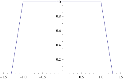
Figure 1.2: A one-dimensional tent function, with $\delta=0.3$

For each $1\leq n\leq d$, we consider the function

$$g^{n}_{\delta}(x)=f\left(\frac{b_{n}-a_{n}}{2}x+\frac{b_{n}+a_{n}}{2}\right).$$

This is a tent function over $[a_{n},b_{n}]$, viz., $g^{n}_{\delta}$ is a continuous function that is 1 on $[a_{n},b_{n}]$ and vanishes outside an interval slightly bigger than $[a_{n},b_{n}]$. Precisely, the decay to zero takes place on the intervals $[a_{n}-(b_{n}-a_{n})\delta/2,a_{n}]$ and $[b_{n},b_{n}+(b_{n}-a_{n})\delta/2]$, so that a similar computation as above yields

$$\|g^{n}_{\delta}-\chi_{[a_{n},b_{n}]}\|_{L^{1}(\mathbb{R})}<(b_{n}-a_{n})\delta.$$ (1.5)

We now set

$$g_{\delta}(x_{1},\ldots,x_{d})=g^{1}_{\delta}(x_{1})\cdots g^{d}_{\delta}(x_{d}).$$

By construction, $g_{\delta}$ is clearly 1 on $Q$ and 0 outside a cube slightly bigger than $Q$. By Tonelli’s theorem and the (1.5), we have

$$\|g_{\delta}-\chi_{Q}\|_{L^{1}(\mathbb{R}^{d})}<\delta^{d}\prod_{n=1}^{d}(b_{n}-a_{n}).$$

Since $\delta$ can be made arbitrarily small, we have successfully produced a continuous approximation of $\chi_{Q}$. This proves the theorem for $p=1$.

We move onto the $p>1$ case. We fix $\varepsilon>0$ and claim that each $f\in L^{p}(\mathbb{R}^{d})$ furnishes a $g\in L^{\infty}(\mathbb{R}^{d})$ and a compact set $K\subseteq(\mathbb{R}^{d})$ such that $\operatorname{supp}g\subseteq K$ and $\|f-g\|_{p}<\varepsilon$. To see this, we define the truncation operator $T_{r}:\mathbb{C}\to\mathbb{C}$ at $r>0$ by setting

$$T_{n}z=\begin{cases}z&\mbox{ if }|z|\leq r;\\ \frac{rz}{|z|}&\mbox{ if }|z|>r;\end{cases}$$

and set

$$f_{n}=\chi_{B_{n}(0)}T_{n}f$$

for each $n\in\mathbb{N}$. The dominated convergence theorem implies that $\|f_{n}-f\|_{p}\to 0$ as $n\to\infty$, and so we can pick an integer $N$ such that $\|f_{N}-f\|_{p}<\varepsilon/2$.

Fix a second constant $\varepsilon_{1}>0$. Since $f_{n}\in L^{1}(\mathbb{R}^{d})$, we can find $g^{\prime}\in\mathscr{C}_{c}(\mathbb{R}^{d})$ such that $\|g^{\prime}-f_{N}\|_{1}<\varepsilon_{1}$. We set $g=T_{\|g\|_{\infty}}g^{\prime}$ and note that

$$g\in\mathscr{C}_{c}(\mathbb{R}^{d}),\hskip 7.22743pt\|g\|_{\infty}\leq\|f_{N}\|_{\infty},\hskip 7.22743pt\mbox{and}\hskip 7.22743pt\|g-f_{N}\|_{1}<\varepsilon_{1}.$$

It now follows from Hölder’s inequality that

$$\|f-g\|_{p} \leq \|f-f_{N}\|_{p}+\|f_{N}-g\|_{p}$$

$$< \frac{\varepsilon}{2}+\|g-g_{1}\|^{1/p}_{1}\|g-g_{1}\|^{1-(1/p)}_{\infty}$$

$$< \frac{\varepsilon}{2}+\varepsilon_{1}^{1/p}\left(2\|g\|_{\infty}\right)^{1-(1/p)},$$

whence picking a sufficiently small $\varepsilon_{1}>0$ yields

$$\|f-g\|_{p}<\varepsilon.$$

This completes the proof of the theorem. ∎

1.2.2 Convolutions

To refine our approximation techniques even further, we now introduce a widely used “smoothing” operation.

Definition 1.15.

The convolution of measurable functions $f$ and $g$ on $\mathbb{R}^{d}$ at $x\in\mathbb{R}^{d}$ is defined to be

$$(f*g)(x)=\int f(x-y)g(y)\,dy,$$

whenever the expression is well-defined.

Convolutions can be thought of as a kind of weighted average. Indeed, if $f(x)=1$, then $f*g$ corresponds to the integral mean value of $g$ over the entire space. Before we discuss why convolutions are smoothing operations, we establish a few basic properties thereof.

Theorem 1.16 (Properties of convolutions).

Let $1\leq p\leq\infty$.

1. The convolution of two measurable functions is measurable.

2. If $f$ and $g$ are measurable, then $f*g=g*f$.

3. Young’s inequality. If $f\in L^{p}(\mathbb{R}^{d})$ and $g\in L^{1}(\mathbb{R}^{d})$, then $f*g$ is well-defined almost everywhere and

   $$\|f*g\|_{p}\leq\|f\|_{p}\|g\|_{1}.$$

The following inequality of Hermann Minkowski, which we shall use frequently in the remainder of the thesis, plays a crucial role in the proof of (c).

Theorem 1.17 (Minkowski’s integral inequality).

Let $(X,\mathfrak{M},\mu)$ and $(Y,\mathfrak{N},\linebreak\nu)$ be $\sigma$-finite measure spaces and $f$ an $(\mu\times\nu)$-measurable function on $X\times Y$. If $f\geq 0$ and $1\leq p<\infty$, then

$$\left(\int\left(\int f(x,y)\,d\nu(y)\right)^{p}\,d\mu(x)\right)^{1/p}\leq\int\left(\int f(x,y)^{p}\,d\mu(x)\right)^{1/p}\,d\nu(y).$$

Proof.

The $p=1$ case is Tonelli’s theorem. If $1<p<\infty$, then Tonelli’s theorem and Hölder’s inequality imply that each $g\in L^{p^{\prime}}(X,\mu)$ satisfies the following inequality:

$$\iint f(x,y)\,d\nu(y)|g(x)|\,d\mu(x) = \iint f(x,y)|g(x)|\,d\mu(x)\,d\nu(y)$$

$$\leq \int\left(\int f(x,y)^{p}\,d\mu(x)\right)^{1/p}\|g\|_{p^{\prime}}\,d\nu(y)$$

$$= \|g\|_{p^{\prime}}\int\left(\int f(x,y)^{p}\,d\mu(x)\right)^{1/p}\,d\nu(y).$$

Let

$$\phi(x)=\int\int f(x,y)\,d\nu(y).$$

We know from the Riesz representation theorem that

$$\|\phi\|_{p}=\sup_{\|g\|_{p^{\prime}}\leq 1}\left|\int\phi g\,d\mu\right|,$$

whence the above inequality implies that

$$\left(\int\left(\int f(x,y)\,d\nu(y)\right)^{p}\,d\mu(x)\right)^{1/p}$$

$$= \|\phi\|_{p}$$

$$= \sup_{\|g\|_{p^{\prime}}\leq 1}\left|\int\phi g\,d\mu\right|$$

$$\leq \sup_{\|g\|_{p^{\prime}}\leq 1}\|g\|_{p^{\prime}}\int\left(\int f(x,y)^{p}\,d\mu(x)\right)^{1/p}\,d\nu(y)$$

$$= \int\left(\int f(x,y)^{p}\,d\mu(x)\right)^{1/p}\,d\nu(y),$$

as was to be shown. ∎

We proceed to the proof of the basic properties of convolutions.

Proof of Theorem 1.16.

(a) Let $f$ and $g$ be measurable functions on $\mathbb{R}^{d}$. We first show that

$$f_{1}(x,y)=f(x-y)$$

is measurable on $\mathbb{R}^{d}\times\mathbb{R}^{d}$. It clearly suffices to prove that $f_{1}^{-1}(B_{r}(z))$ is measurable for each $r>0$ and every $z\in\mathbb{C}$. For each subset $E$ of $\mathbb{R}^{d}$, we define

$$\tilde{E}=\{(x,y)\in\mathbb{R}^{d}\times\mathbb{R}^{d}:x-y\in E\}.$$

Since the subtraction operation

$$(x,y)\mapsto x-y$$

is a continuous map from $\mathbb{R}^{d}\times\mathbb{R}^{d}$ into $\mathbb{R}^{d}$, the set $\tilde{E}$ is open whenever $E$ is open. By taking a countable intersection, we see that $\tilde{E}$ is a $G_{\delta}$ set if $E$ is.

We also claim that $\tilde{E}$ is of measure zero whenever $E$ is of measure zero. Indeed, if $|E|=0$, then we can find a sequence $(O_{n})_{n=1}^{\infty}$ of open sets such that $O_{n}\supseteq E$ for each $n$ and $|O_{n}|\to 0$ as $n\to\infty$. Given $n,k\in\mathbb{N}$, Tonelli’s theorem and the translation invariance of the Lebesgue measure imply that

$$|\tilde{O}_{n}\cap B_{k}(0)| = \iint\chi_{O_{n}}(x-y)\chi_{B_{k}(0)}(y)\,dy\,dx$$

$$= \int\left(\int\chi_{O_{n}}(x-y)\,dx\right)\chi_{B_{k}(0)}\,dy$$

$$= \int\left(\int\chi_{O_{n}}(x)\,dx\right)\chi_{B_{k}(0)}\,dy$$

$$= |O_{n}||B_{k}|.$$

Therefore, if we set $\tilde{E}_{k}=\tilde{E}\cap B_{k}(0)$ for each positive integer $k$, then $\tilde{E}_{k}\subseteq\tilde{O}_{n}\cap B_{k}(0)$ for all $n$ and $|\tilde{O}_{n}\cap B_{k}(0)|\to 0$ as $n\to\infty$. It follows that $|\tilde{E}_{k}|=0$, whence by continuity of measure we have $|\tilde{E}|=0$, as desired.

We now fix an $r>0$ and a $z\in\mathbb{C}$ and set $E=f^{-1}(B_{r}(z))$, so that $\tilde{E}=f_{1}^{-1}(B_{r}(z))$. Since $B_{r}(z)$ is open, the measurability of $f$ implies the measurability of $E$, whence Proposition 1.7 furnishes a $G_{\delta}$ set $G$ such that $G\supseteq E$ and $|G\smallsetminus E|=0$. Setting $F=G\smallsetminus E$, we see that

$$\tilde{G}=\tilde{E}\cup\tilde{F}$$

is a $G_{\delta}$ set. Since $|F|=0$, the above argument shows that $|\tilde{F}|=0$, whereby we appeal once again to Proposition 1.7 to conclude that $\tilde{E}$ is measurable.

It follows that if $f$ and $g$ are measurable functions on $\mathbb{R}^{d}$, then

$$(x,y)\mapsto f(x-y)g(y)$$

is measurable on $\mathbb{R}^{d}\times\mathbb{R}^{d}$. We now invoke Fubini’s theorem to conclude that

$$(f*g)(x)=\int f(x-y)g(y)\,dy$$

is measurable on $\mathbb{R}^{d}$.

(b) This is a trivial consequence of the commutativity of multiplication in $\mathbb{C}$ and the translation invariance of the Lebesgue measure.

(c) Since $|(f*g)(x)|\leq\int|f(x-y)||g(y)|\,dy$, we invoke Minkowski’s integral inequality to conclude that

$$\|f*g\|_{p} = \left(\int\left|\int f(x-y)g(y)\,dy\right|^{p}\,dx\right)^{1/p}$$

$$\leq \int\left(\int|f(x-y)|^{p}\,dx\right)^{1/p}|g(y)|\,dy$$

$$= \|f\|_{p}\|g\|_{1},$$

as was to be shown. ∎

We now return to the task of justifying the “smoothing operator” nickname that convolutions possess. We begin by showing that the convolution of two compactly supported functions is compactly supported.

Theorem 1.18.

Let $1\leq p\leq\infty$. If $f\in L^{p}(\mathbb{R}^{d})$ and $g\in L^{1}(\mathbb{R}^{d})$, then

$$\operatorname{supp}(g*h)\subseteq\overline{\operatorname{supp}f+\operatorname{supp}g}=\overline{\{x+y:x\in\operatorname{supp}f\mbox{ and }y\in\operatorname{supp}g\}}$$

As it stands now, however, it is not entirely clear how we should interpret the statement of the above theorem. While two functions that are almost everywhere are considered to be “the same” in integration theory, the traditional notion of support can fail to assign the same support to both functions. To rectify this issue, we adopt a new definition:

Definition 1.19.

Let $f$ be a complex-valued function on $\mathbb{R}^{d}$ and $O$ the union of all open sets in $\mathbb{R}^{d}$ on which $f$ vanishes almost everywhere. We define the support of $f$, denoted $\operatorname{supp}f$, to be the complement of $O$.

Of course, we must justify the new terminology:

Proposition 1.20.

Let $f$ and $O$ be defined as above. Then $f$ vanishes almost everywhere on $O$. If $g$ is another function that is equal to $f$ almost everywhere, then $\operatorname{supp}f=\operatorname{supp}g$. Furthermore, this definition of support agrees with the old definition of support for continuous functions.

Proof.

Since $\mathbb{R}^{d}$ is second-countable, we can find a sequence $(O_{n})_{n=1}^{\infty}$ of of open sets such that $f$ vanishes almost everywhere on each $O_{n}$ and that the union of all $O_{n}$ is $O$. The union is countable, and so $f$ vanishes almost everywhere on $O$. If $f=g$ almost everywhere, then $f$ vanishes almost everywhere on a vanishing set of $g$, and vice versa, whence $\operatorname{supp}f$ and $\operatorname{supp}g$ must agree. If $f$ is continuous, then $O=f^{-1}(\mathbb{C}\smallsetminus\{0\})$, and so $\operatorname{supp}f=f^{-1}(\{0\})$, as was to be shown. ∎

With the new definition, we proceed to the proof of the theorem.

Proof of Theorem 1.18.

By Young’s inequality, the map $y\mapsto f(x-y)g(y)$ is integrable for each $x\in\mathbb{R}^{d}$. Writing $x-\operatorname{supp}f$ to denote the set $\{x-y:y\in\operatorname{supp}f\}$, we see that

$$(f*g)(x)=\int_{(x-\operatorname{supp}f)\cap\operatorname{supp}g}f(x-y)g(y)\,dy.$$

Let $E=\operatorname{supp}f+\operatorname{supp}g$ for notational simplicity. We note that $x\notin E$ implies $(x-\operatorname{supp}f)\cap\operatorname{supp}g=\varnothing$, so that $(f*g)(x)=0$. Therefore, $(f*g)(x)=0$ for almost every $x\in\mathbb{R}^{d}\smallsetminus E$. In particular, $(f*g)(x)=0$ for almost every $x$ in the interior of $\mathbb{R}^{d}\smallsetminus E$, and so

$$\operatorname{supp}(f*g)\subseteq\overline{E}$$

by the new definition of support. ∎

We are now ready to supply the promised justification of the smoothing-operations nickname. For notational simplicity we define the following shorthand:

Definition 1.21.

A $d$-dimensional multi-index is a $d$-tuple

$$\alpha=(\alpha_{1},\ldots,\alpha_{d})$$

consisting of nonnegative integers. We employ the following notations for multi-indices; here $\alpha$ and $\beta$ are multi-indices, and $x$ an element of $\mathbb{R}^{d}$:

$$|\alpha| = \alpha_{1}+\cdots+\alpha_{d}$$

$$x^{\alpha} = x_{1}^{\alpha_{1}}\cdots x_{d}^{\alpha_{d}}$$

$$D^{\alpha} = \left(\frac{\partial}{\partial x_{1}}\right)^{\alpha_{1}}\cdots\left(\frac{\partial}{\partial x_{d}}\right)^{\alpha_{d}}$$

$$\alpha\pm\beta = (\alpha_{1}\pm\beta_{1},\cdots,\alpha_{d}\pm\beta_{d}).$$

The main theorem can now be stated as follows:

Theorem 1.22 (Convolution as a smoothing operation).

Convolutions are “smoothing operations” in the following sense:

1. If $f\in\mathscr{C}_{c}(\mathbb{R}^{d})$ and $g\in L^{1}_{\operatorname{loc}}(\mathbb{R}^{d})$, then $f*g$ is well-defined everywhere and $f*g\in\mathscr{C}(\mathbb{R}^{d})$.

2. If $f\in\mathscr{C}^{k}_{c}(\mathbb{R}^{d})$ and $g\in L^{1}_{\operatorname{loc}}(\mathbb{R}^{d})$, then $f*g\in\mathscr{C}^{k}(\mathbb{R}^{d})$ and

   $$D^{\alpha}(f*g)=(D^{\alpha}f)*g$$

   for each multi-index $|\alpha|\leq k$. The result holds for $k=\infty$ as well.

3. If $f\in\mathscr{C}^{k}(\mathbb{R}^{d})$ and $g\in\mathscr{C}^{l}(\mathbb{R}^{d})$, then $f*g\in\mathscr{C}^{k+l}(\mathbb{R}^{d})$ and

   $$D^{\alpha+\beta}(f*g)=(D^{\alpha}f)*(D^{\beta}g)$$

   for all multi-index $|\alpha|\leq k$ and $|\beta|\leq l$.

Proof.

(a) For each $x\in\mathbb{R}^{d}$, the map $x\mapsto f(x-y)g(y)$ is measurable and has compact support, hence integrable. Therefore, $(f*g)(x)$ is defined for all $x\in\mathbb{R}^{d}$. We now fix $x\in\mathbb{R}^{n}$, pick a sequence $(x_{n})_{n=1}^{\infty}$ in $\mathbb{R}^{d}$ converging to $x$, and find a compact subset $K$ of $\mathbb{R}^{d}$ such that

$$x_{n}-\operatorname{supp}f=\{x_{n}-y:y\in\operatorname{supp}f\}\subseteq K$$

for each $n\in\mathbb{N}$. It then follows that $f$ is uniformly continuous on $K$ and $f(x_{n}-y)=0$ for all $n\in\mathbb{N}$ and $y\in\mathbb{R}^{d}\smallsetminus K$. We can thus pick a sequence $(\varepsilon_{n})_{n=1}^{\infty}$ of positive real numbers converging to zero such that

$$|f(x_{n}-y)-f(x-y)|\leq\varepsilon_{n}\chi_{K}(y)$$

for each $n\in\mathbb{N}$ and every $y\in\mathbb{R}^{d}$. Multiplying through by $|g(y)|$ and integrating with respect to $y$, we obtain

$$|(f*g)(x_{n})-(f*g)(x)|\leq\varepsilon_{n}\int_{K}|g(y)|\,dy.$$

Since the right-hand side converges to zero as $n\to\infty$, we conclude that

$$\lim_{n\to\infty}(f*g)(x_{n})=(f*g)(x),$$

as was to be shown.

(b) We suppose for now that $k=1$. The task at hand then reduces to establishing the claim that $f*g$ is continuously differentiable at each $x\in\mathbb{R}^{d}$ and

$$\nabla(f*g)(x)=(\nabla f*g)(x).$$

To this end, we pick $x\in\mathbb{R}^{d}$. For each $y\in\mathbb{R}^{d}$, we observe that

$$\lim_{|h|\to 0}\frac{|f((x-y)+h)-f(x-y)-\nabla f(x-y)\cdot h|}{|h|}=0,$$

whence every $\varepsilon>0$ admits $M_{\varepsilon}>0$ such that

$$|f((x-y)+h)-f(x-y)-\nabla f(x-y)\cdot h|\leq\varepsilon|h|$$

for all $|h|<M_{\varepsilon}$.

Fix a compact subset $K$ of $\mathbb{R}^{d}$ such that

$$x-\operatorname{supp}f+B_{M_{\varepsilon}}(0)=\{(x-y)+h:y\in\operatorname{supp}f\mbox{ and }|h|<M_{\varepsilon}\}\subseteq K.$$

Since

$$f((x-y)+h)-f(x-y)-\nabla f(x-y)\cdot h=0$$

for all $|h|<M_{\varepsilon}$ and $y\in K$, we have

$$|f((x-y)+h)-f(x-y)-\nabla f(x-y)\cdot h|\leq\varepsilon|h|\chi_{K}(y)$$

for all $y\in\mathbb{R}^{d}$. Multiplying through by $|g(y)|$ and integrating with respect to $y$, we see that

$$|(f*g)(x+h)-(f*g)(x)-(\nabla f*g)(x)\cdot h|\leq\varepsilon|h|\int_{K}|g(y)|\,dy.$$

It follows that $f*g$ is differentiable at $x$, with the gradient

$$\nabla(f*g)(x)=(\nabla f*g)(x).$$

$f\in\mathscr{C}^{1}_{c}(\mathbb{R}^{d})$ implies that $\nabla f\in\mathscr{C}_{c}(\mathbb{R}^{d})$, whence $\nabla f*g\in\mathscr{C}(\mathbb{R}^{d})$ by (a). This completes the proof for $k=1$. The case for $k>1$ now follows from induction.

(c) is a trivial consequence of (b) and the commutativity of convolution, and the proof is now complete. ∎

1.2.3 Approximation by Smooth Functions

We shall now establish the final approximation theorem of this section: namely, the approximation of $L^{p}$ functions by smooth functions. As was hinted at in the previous subsection, we shall use convolutions to smooth out the approximating functions. The key result, known as approximations to the identity, provides a widely applicable tool for generating a collection of approximating functions for any given $L^{p}$ function.

Theorem 1.23 (Approximations to the identity).

Let $1\leq p<\infty$. If $f\in L^{p}(\mathbb{R}^{d})$ and $\rho\in L^{1}(\mathbb{R}^{d})$ such that $\int\rho=1$, then $\|f*\rho_{\varepsilon}-f\|_{p}\to 0$ as $\varepsilon\to 0$, where $\rho_{\varepsilon}(x)=\varepsilon^{-d}\rho(\varepsilon^{-1}x)$ for each $\varepsilon>0$.

As per Theorem 1.22, we can make the approximating functions as well-behaved as we would like. Indeed, we can construct smooth approximations to the identity, which we shall furnish after the proof of the theorem.

Proof.

We set $\Delta_{f}(y)=\|f(x-y)-f(x)\|_{p}$ for each $y\in\mathbb{R}^{d}$. Fix $\delta>0$ and invoke Theorem 1.14 to find $f_{1}\in\mathscr{C}_{c}(\mathbb{R}^{d})$ with $\|f-f_{1}\|_{p}\leq\delta$. Set $f_{2}=f-f_{1}$. Since $f_{1}(x-y)$ converges uniformly to $f_{1}(x)$ as $y\to 0$, we see that $\Delta_{f_{1}}(y)\to 0$ as $y\to 0$. Moreover, $\Delta_{f_{2}}(y)\leq 2\delta$, whence

$$\Delta_{f}(y)\leq\Delta_{f_{1}}(y)+\Delta_{f_{2}}(y)\to 0$$

as $y\to 0$. By Minkowski’s integral inequality, we have the following estimate:

$$\|f*\rho_{\varepsilon}-f\|_{p} = \left\|\int f(x-y)\rho_{\varepsilon}(y)\,dy-f(x)\right\|_{p}$$

$$= \left\|\int f(x-y)\rho_{\varepsilon}(y)\,dy-f(x)\int\rho_{\varepsilon}(y)\,dy\right\|_{p}$$

$$= \left\|\int[f(x-y)-f(x)]\rho_{\varepsilon}(y)\,dy\right\|_{p}$$

$$\leq \int\|f(x-y)-f(x)\|_{L^{p}(x)}|\rho_{\delta}(y)|\,dy$$

$$= \int\Delta_{f}(y)|\rho_{\varepsilon}(y)|\,dy$$

$$= \int\Delta_{f}(\varepsilon y)|\rho(y)|\,dy;$$

the last inequality follows from the change-of-variables formula.

We have shown above that $\Delta_{f}(\varepsilon y)\to 0$ as $\varepsilon\to 0$. Furthermore, we have the bound

$$|\Delta_{f}(\delta y)\rho(y)|\leq\|2f\|_{p}|\rho(y)|,$$

whence by the dominated convergence theorem we obtain

$$\lim_{\varepsilon\to 0}\|f*\rho_{\varepsilon}-f\|_{p} \leq \lim_{\varepsilon\to 0}\int\Delta_{f}(\varepsilon y)|\rho(y)|\,dy$$

$$= \int\lim_{\varepsilon\to 0}\Delta_{f}(\varepsilon y)|\rho(y)|\,dy,$$

as was to be shown. ∎

Corollary 1.24 (Smooth approximations to the identity).

There exists a sequence of mollifiers on $\mathbb{R}^{d}$, which is a sequence $(\rho_{n})_{n=1}^{\infty}$ of nonnegative $\mathscr{C}^{\infty}$-maps on $\mathbb{R}^{d}$ such that $\operatorname{supp}\rho_{n}\subseteq\overline{B_{1/n}(0)}$ and $\int\rho_{n}=1$ for each $n\in\mathbb{N}$. Furthermore, if $f\in L^{p}(\mathbb{R}^{d})$, then $\|f*\rho_{n}-f\|_{p}\to 0$ as $n\to\infty$.

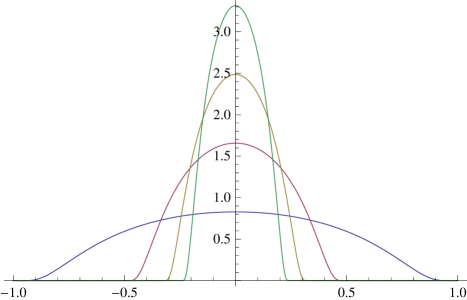
Figure 1.3: The first four mollifiers

Proof.

We set

$$\phi(x)=\begin{cases}e^{1/(|x|^{2}-1)}&\mbox{ if }|x|<1;\\ 0&\mbox{ if }|x|\geq 1\end{cases}$$

and

$$\phi_{\varepsilon}(x)=\frac{\varepsilon^{-d}\phi(\varepsilon^{-1}x)}{\int\phi(x)\,dx}.$$

for each $\varepsilon>0$ Then each $\phi_{\varepsilon}$ is a compactly supported smooth function whose integral is 1, whence by Theorem 1.23 we have

$$\lim_{\varepsilon\to 0}\|f*\rho_{\varepsilon}-f\|_{p}=0.$$

We now define a sequence $(\rho_{n})_{n=1}^{\infty}$ of functions by setting $\rho_{n}=\phi_{1/n}$ for each $n\in\mathbb{N}$. It immediately follows from the above construction that this is a sequence of mollifiers. ∎

The approximation theorem now follows as a simple corollary.

Corollary 1.25.

$\mathscr{C}^{\infty}_{c}(\mathbb{R}^{d})$ is dense in $L^{p}(\mathbb{R}^{d})$ for each $1\leq p<\infty$.

Proof.

Fix $1\leq p<\infty$. Let $(\rho_{n})_{n=1}^{\infty}$ be a sequence of mollifiers, set $B_{n}=\overline{B_{n}(0)}$ for each $n\in\mathbb{N}$, and define a sequence $(f_{n})_{n=1}^{\infty}$ by

$$f_{n}=(f\chi_{B_{n}})*\rho_{n}.$$

Then Young’s inequality implies that

$$\|f-f_{n}\|_{p} \leq \|f-f*\rho_{n}\|_{p}+\|\rho_{n}*f-\rho_{n}*(f\chi_{B_{n}})\|_{p}$$

$$= \|f-f*\rho_{n}\|_{p}+\|\rho_{n}*(f-f\chi_{B_{n}})\|_{p}$$

$$\leq \|f-f*\rho_{n}\|_{p}+\|f-f\chi_{B_{n}}\|_{p}\|\rho_{n}\|_{1}$$

$$= \|f-f*\rho_{n}\|_{p}+\|f-f\chi_{B_{n}}\|_{p}.$$

By Corollary 1.24, we have $\|f-(f*\rho_{n})\|_{p}\to 0$ as $n\to\infty$, and the dominated convergence theorem implies that $\|f-f\chi_{B_{n}}\|_{p}\to 0$ as $n\to\infty$. It follows that

$$\lim_{n\to\infty}\|f-f_{n}\|_{p}=0,$$

as was to be shown. ∎

We conclude the section with another instant of convolutions as smoothing operations. This time, we are able to recover continuity without any smoothness on either side.

Corollary 1.26.

Let $1<p<\infty$. If $f\in L^{p}(\mathbb{R}^{d})$ and $g\in L^{p^{\prime}}(\mathbb{R}^{d})$, then $f*g$ belongs to the space $\mathscr{C}_{0}(\mathbb{R}^{d})$ of continuous functions vanishing at infinity.

Proof.

By Hölder’s inequality, $f*g$ is well-defined everywhere on $\mathbb{R}^{d}$. For each $\varepsilon>0$, Corollary 1.25 furnishes $f_{\varepsilon},g_{\varepsilon}\in\mathscr{C}^{\infty}_{c}(\mathbb{R}^{d})$ such that

$$\|f-f_{\varepsilon}\|_{p}\leq\frac{\varepsilon}{2(\|f\|_{p}+\|g\|_{p^{\prime}})}\hskip 14.45377pt\mbox{and}\hskip 14.45377pt\|g-g_{\varepsilon}\|_{p^{\prime}}\leq\frac{\varepsilon}{2(\|f\|_{p}+\|g\|_{p^{\prime}})}.$$

It then follows from Hölder’s inequality that

$$\|f*g-f_{\varepsilon}*g_{\varepsilon}\|_{\infty} \leq \|(f-f_{\varepsilon})*g\|_{\infty}+\|f_{\varepsilon}*(g-g_{\varepsilon})\|_{\infty}$$

$$\leq \left\|\|f-f_{\varepsilon}\|_{p}\|g\|_{p^{\prime}}\right\|_{\infty}+\left\|\|f_{\varepsilon}\|_{p}\|g-g_{\varepsilon}\|_{p^{\prime}}\right\|_{\infty}$$

$$\leq \|f-f_{\varepsilon}\|_{p}\|g\|_{p^{\prime}}+\|f_{\varepsilon}\|_{p}\|g-g_{\varepsilon}\|_{p^{\prime}}$$

$$\leq (\|f\|_{p}+\|g\|_{p^{\prime}})(\|f-f_{\varepsilon}\|_{p}+\|g-g_{\varepsilon}\|_{p^{\prime}}$$

$$\leq (\|f\|_{p}+\|g\|_{p^{\prime}})\left(\frac{2\varepsilon}{2(\|f\|_{p}+\|g\|_{p^{\prime}})}\right)$$

$$= \varepsilon,$$

whence $f*g$ is a uniform limit of smooth functions $f_{\varepsilon}*g_{\varepsilon}$ with compact support. This establishes the corollary. ∎

1.3 The Fourier Transform

We now restrict our attention to the famous operator of Joseph Fourier, the Fourier transform. To motivate the definition, we consider the “limiting case” of the classical Fourier series

$$\sum_{n=-\infty}^{\infty}\hat{f}(n)e^{2\pi inx/L},$$

of $L$-periodic functions $f:[-L/2,L/2]\to\mathbb{R}$, whose Fourier coefficients are given by the formula

$$\hat{f}(n)=\frac{1}{L}\int_{-L/2}^{L/2}f(x)e^{-2\pi inx/L}\,dx$$

Indeed, we make a simple change of variable in the above formula to obtain

$$\hat{f}(n)=\int_{-1/2}^{1/2}f(Lx)e^{-2\pi inx}\,dx,$$

and “sending $L$ to infinity” leads us to the following:

$$\hat{f}(n)=\int_{-\infty}^{\infty}f(x)e^{-2\pi inx}\,dx.$$

So long as $f$ decays suitably at infinity, the integral makes sense even when $n$ is not an integer. Therefore, we replace $n$ with a real variable $\xi$:

$$\hat{f}(\xi)=\int_{-\infty}^{\infty}f(x)e^{-2\pi i\xi x}\,dx.$$

We promptly generalize the above “transform” to higher dimensions; this, of course, requires us to take the scalar product of multi-dimensional variables $x$ and $\xi$, which we do by taking the standard dot product:

$$\hat{f}(\xi)=\int_{\mathbb{R}^{d}}f(x)e^{-2\pi i\xi\cdot x}\,dx.$$

1.3.1 The $L^{1}$ Theory

The above expression makes sense only if $f(x)e^{-2\pi i\xi\cdot x}$ is in $L^{1}$ for all $\xi$. Since $|e^{-2\pi i\xi\cdot x}|=1$ for all $x$ and $\xi$, this is equivalent to the condition that $f$ is in $L^{1}(\mathbb{R}^{d})$. We are thus led to the following definition:

Definition 1.27.

The Fourier transform of $f\in L^{1}(\mathbb{R}^{d})$ is the function $\hat{f}$ given by

$$\hat{f}(\xi)=\int f(x)e^{-2\pi i\xi\cdot x}\,dx$$

for each $\xi\in\mathbb{R}^{d}$. We also write $\mathscr{F}f$ to denote the Fourier transform of $f$.

Note that $\mathscr{F}$ can be thought of as an operator on $L^{1}(\mathbb{R}^{d})$. By the linearity of the integral, $\mathscr{F}$ is a linear operator. The target space of $\mathscr{F}$, as well as a few other basic properties of $\mathscr{F}$, are established in the following proposition.

Proposition 1.28.

The Fourier transform of $f\in L^{1}(\mathbb{R}^{d})$ satisfies the following properties:

1. $\|\hat{f}\|_{\infty}\leq\|f\|_{1}$. Therefore, $\mathscr{F}$ is a bounded linear operator from $L^{1}(\mathbb{R}^{d})$ into $L^{\infty}(\mathbb{R}^{d})$.

2. $\hat{f}$ is uniformly continuous on $\mathbb{R}^{d}$.

3. Riemann-Lebesgue lemma. $\hat{f}$ vanishes at infinity, viz., $\hat{f}(\xi)\to 0$ as $|\xi|\to\infty$.

Proof.

(a) It suffices to observe that

$$\|\hat{f}\|_{\infty}=\left\|\int f(x)e^{-2\pi i\xi\cdot x}\,dx\right\|_{\infty}\leq\int|f(x)||e^{-2\pi i\xi\cdot x}|\,dx\leq\|f\|_{1}.$$

(b) Since $|f(x+h)-f(x)|\leq 2|f(x)|$ for all sufficiently small $h\in\mathbb{R}^{d}$, it follows from the dominated convergence theorem that

$$\lim_{h\to infty}|\hat{f}(\xi+h)-\hat{f}(\xi)| \leq \lim_{h\to infty}\int|f(x+h)-f(x)||e^{-2\pi i\xi\cdot x}|\,dx$$

$$= \int\lim_{h\to infty}|f(x+h)-f(x)|\,dx$$

$$= 0.$$

(c) Let $Q=[0,1]^{d}$. By Tonelli’s theorem,

$$\widehat{\chi_{Q}(\xi)}=\int\chi_{Q}(x)e^{-2\pi i\xi\cdot x}\,dx=\prod_{n=1}^{d}\int_{0}^{1}e^{-2\pi ix_{n}\xi_{n}}\,dx_{n}=\prod_{n=1}^{d}\frac{e^{-2\pi i\xi}-1}{-2\pi i\xi},$$

which tends to zero as $|\xi|\to\infty$. By linearity, the Riemann-Lebesgue lemma holds for all simple functions over cubes. Given a general integrable function $f$ on $\mathbb{R}^{d}$, we can invoke Theorem 1.13 to find a simple function $s_{\varepsilon}$ over cubes corresponding to each $\varepsilon>0$, satisfying the estimate

$$\|f-f_{\varepsilon}\|_{1}<\varepsilon.$$

Since $\hat{f_{\varepsilon}}(\xi)\to 0$ as $|\xi|\to\infty$, we can find a constant $M$ such that $|\hat{f_{\varepsilon}}(\xi)|<\varepsilon$ for all $|\xi|>M$. It then follows that

$$|\hat{f}(\xi)| \leq |\widehat{f_{\varepsilon}}(\xi)|+\int|f(x)-f_{\varepsilon}(x)||e^{-2\pi i\xi\cdot x}|\,dx$$

$$= |\widehat{f_{\varepsilon}}(\xi)|+\|f-f_{\varepsilon}\|_{\varepsilon}$$

$$\leq 2\varepsilon$$

for all $|\xi|>M$, whence $\hat{f}(\xi)\to 0$ as $|\xi|\to\infty$. ∎

The Fourier transform behaves well under a number of symmetry operations in the Euclidean space. The proof of the following proposition consists of trivial computations and is thus omitted.

Proposition 1.29.

Let $f\in L^{1}(\mathbb{R}^{d})$ and $\tau\in\mathbb{R}^{d}$.

1. $\mathscr{F}$ turns translation into rotation: if $\tau_{h}f(x)=f(x-h)$, then

   $$\widehat{\tau_{h}f}(\xi)=e^{-2\pi ih\cdot\xi}\hat{f}(\xi).$$

2. $\mathscr{F}$ turns rotation into translation: if $e_{h}f(x)=e^{2\pi ix\cdot h}f(x)$, then

   $$\widehat{e_{h}f}(\xi)=\tau_{h}\hat{f}(\xi).$$

3. $\mathscr{F}$ commutes with reflection: if $\tilde{f}(x)=f(-x)$, then

   $$\hat{\tilde{f}}(\xi)=\tilde{\hat{f}}(\xi).$$

4. $\mathscr{F}$ scales nicely under dilation: if we set $\delta_{a}f(x)=f(ax)$ for each $a>0$, then

   $$\widehat{\delta_{a}f}(\xi)=a^{-d}\delta_{a^{-1}}\hat{f}(\xi)=a^{-d}\hat{f}(a^{-1}\xi)$$

   for all $a>0$. ∎

The Fourier transform also behaves quite nicely under differentiation. Indeed, the Fourier transform turns differentiation into multiplication by a polynomial.

Proposition 1.30.

Let $f\in L^{1}(\mathbb{R}^{d})$ and suppose that $x_{n}f(x_{1},\ldots,x_{n},\ldots,x_{d})$ is an $L^{1}$ function as well. Then $\hat{f}(\xi_{1},\ldots,\xi_{n},\ldots,x_{d})$ is continuously differentiable with respect to $\xi_{n}$ and

$$\frac{\partial}{\partial\xi_{k}}\hat{f}(\xi)=\mathscr{F}(-2\pi ix_{n}f(x))(\xi).$$

More generally, if $P$ is a polynomial in $d$ variables, then

$$P(D)\hat{f}(\xi)=\mathscr{F}(P(-2\pi ix)f(x))(\xi)\hskip 14.45377pt\mbox{and}\hskip 14.45377pt\mathscr{F}(P(D)f)(\xi)=P(2\pi i\xi)\hat{f}(\xi).$$

Proof.

Let $h=(0,\ldots,h_{n},\ldots,0)$ be a nonzero vector along the $n$th coordinate axis. By Proposition 1.29 (ii) and the dominated convergence theorem, we have

$$\lim_{h_{n}\to 0}\frac{\hat{f}(\xi+h)-\hat{f}(\xi)}{h_{n}} = \lim_{h_{n}\to 0}\mathscr{F}\left(\left(\frac{e^{-2\pi ix\cdot h}-1}{h_{n}}\right)f(x)\right)(\xi)$$

$$= \mathscr{F}(-2\pi ix_{n}f(x))(\xi),$$

as was to be shown. The second assertion now follows from linearity of the differential operator. ∎

To rid ourselves of technical issues that arise in dealing with non-smooth functions, it will be convenient to work in a space of smooth functions that behaves well under the key operations in harmonic analysis. Certainly, we would like the space to be closed under the Fourier transform. Proposition 1.30 then implies that the space must be closed under multiplication by polynomials as well. We are thus led to the following definition, named after Laurent Schwartz:

Definition 1.31.

The Schwartz space $\mathscr{S}(\mathbb{R}^{d})$ consists of functions $f\in\mathscr{C}^{\infty}(\mathbb{R}^{d})$ with the decay condition

$$\sup_{x\in\mathbb{R}^{d}}|x^{\alpha}D^{\beta}f(x)|<\infty$$

for each pair of multi-indices $\alpha$ and $\beta$.

We remark that

$$\mathscr{C}_{c}^{\infty}(\mathbb{R}^{d})\subseteq\mathscr{S}(\mathbb{R}^{d})\subseteq L^{p}(\mathbb{R}^{d})$$

for all $1\leq p\leq\infty$. Since $\mathscr{C}^{\infty}_{c}(\mathbb{R}^{d})$ contains mollifiers, $\mathscr{S}(\mathbb{R}^{d})$ is nonempty. In fact, $\mathscr{C}^{\infty}_{c}(\mathbb{R}^{d})$ is dense in $L^{p}(\mathbb{R}^{d})$, whence so is $\mathscr{S}(\mathbb{R}^{d})$.

An equivalent definition for a Schwartz function is a function $f\in\mathscr{C}^{\infty}(\mathbb{R}^{d})$ that satisfies the growth condition

$$\sup_{x\in\mathbb{R}^{d}}\langle x\rangle^{n}|D^{\alpha}f(x)|<\infty$$

for all natural numbers $n$ and multi-indices $\alpha$, where

$$\langle x\rangle=\sqrt{1+x^{2}}.$$

As noted, the Schwartz space is closed under the action of the Fourier transform. This basic fact is an immediate corollary of Proposition 1.30.

Proposition 1.32.

If $f\in\mathscr{S}(\mathbb{R}^{d})$, then $\hat{f}\in\mathscr{S}(\mathbb{R}^{d})$. ∎

The Schwartz space behaves well under other important operations in harmonic analysis as well. We shall take up this matter in §2.3.

We now turn to one of the fundamental questions in classical Fourier analysis: given the Fourier transform of a function, can we find the function itself? We begin with a useful proposition that allows us to “push the hat around”:

Proposition 1.33 (Multiplication formula).

If $f,g\in L^{1}(\mathbb{R}^{d})$, then

$$\int\hat{f}(t)g(t)\,dt=\int f(t)\hat{g}(t)\,dt.$$

Proof.

By Fubini’s theorem,

$$\int\hat{f}(t)g(t)\,dt = \int\left(\int f(x)e^{-2\pi it\cdot x}\,dx\right)g(t)\,dt$$

$$= \int\left(\int g(t)e^{-2\pi it\cdot x}\,dt\right)f(x)\,dx$$

$$= \int\hat{g}(x)f(x)\,dx$$

$$= \int f(t)\hat{g}(t)\,dt,$$

as desired. ∎

We shall also need the following computation:

Proposition 1.34.

For all $\varepsilon>0$, we have

$$\mathscr{F}\left(e^{-\varepsilon\pi|x|^{2}}\right)(\xi)=\varepsilon^{-d/2}e^{-\varepsilon^{-1}\pi|\xi|^{2}}.$$

This, in particular shows that the Fourier transform of the Gaussian

$$\Gamma(x)=e^{-\pi|x|^{2}}$$

is the Gaussian itself.

Proof.

Recall that

$$\int_{-\infty}^{\infty}e^{-x^{2}}dx=\sqrt{\pi}.$$

We first consider the one-dimensional case. In fact, we fix positive real numbers $p$ and $q$ and compute a more general integral:

$$\int_{-\infty}^{\infty}e^{-px^{2}}e^{-qix}\,dx = \int_{-\infty}^{\infty}e^{-p(x^{2}+\frac{qi}{p}x)}\,dx$$

$$= \int_{-\infty}^{\infty}e^{-p(x+\frac{qi}{2p})^{2}-\frac{q^{2}}{4p}}\,dx$$

$$= e^{-q^{2}/4p}\int_{-\infty}^{\infty}e^{-p(x+\frac{qi}{2p})^{2}}$$

$$= e^{-q^{2}/4p}\int_{-\infty}^{\infty}e^{-(\sqrt{p}x)^{2}}$$

$$= \frac{e^{-q^{2}/4p}}{\sqrt{p}}\int_{-\infty}^{\infty}e^{-x^{2}}$$

$$= e^{-q^{2}/4p}\sqrt{\frac{\pi}{p}}.$$

Plugging in $p=\varepsilon\pi$ and $q=2\pi\xi$, we have

$$\mathscr{F}\left(e^{-\varepsilon\pi x^{2}}\right)(\xi)=\varepsilon^{-1/2}e^{-\varepsilon^{-1}\pi\xi^{2}}$$

whenever $x,\xi\in\mathbb{R}$.

It now suffices to observe that

$$\mathscr{F}\left(e^{-\varepsilon\pi|x|^{2}}\right)(\xi) = \int e^{-\varepsilon\pi|x|^{2}}e^{-2\pi i\xi\cdot x}\,dx$$

$$= \prod_{n=1}^{d}\int e^{-\varepsilon\pi x_{n}^{2}}e^{-2\pi i\xi_{n}x_{n}}\,dx_{n}$$

$$= \prod_{n=1}^{d}\mathscr{F}\left(e^{-\varepsilon\pi x_{n}^{2}}\right)(\xi_{n})$$

$$= \prod_{n=1}^{d}\varepsilon^{-1/2}e^{-\varepsilon^{-1}\pi\xi_{n}^{2}}$$

$$= \varepsilon^{-d/2}e^{-\varepsilon^{-1}\pi|\xi|^{2}},$$

as desired. ∎

We now present a preliminary solution to the inversion problem, which is sufficient for the present thesis. A more detailed discussion can be found in §§2.7.6.

Theorem 1.35 (Fourier inversion theorem).

If $f\in L^{1}(\mathbb{R}^{d})$ and $\hat{f}\in L^{1}(\mathbb{R}^{d})$, then

$$f(x)=\int\hat{f}(\xi)e^{2\pi i\xi\cdot x}\,d\xi$$

for almost every $x\in\mathbb{R}^{d}$.

By Proposition 1.32, Schwartz functions satisfy the hypothesis of the above theorem. In general, Proposition 1.28 indicates that $f$ must necessarily be a $C_{0}$ map, although this is not a sufficient condition.

Proof of Theorem 1.35.

We consider the following modification of the inversion theorem:

$$I_{\varepsilon}(x)=\int\hat{f}(\xi)e^{-\pi\varepsilon^{2}|\xi|^{2}}e^{2\pi i\xi\cdot x}\,d\xi.$$

Since $\hat{f}\in L^{1}(\mathbb{R}^{d})$, the dominated convergence theorem implies that

$$\lim_{\varepsilon\to 0}I_{\varepsilon}(x)=\int\hat{f}(\xi)e^{2\pi i\xi\cdot x}\,d\xi.$$

We now set $g_{\varepsilon}(\xi)=e^{-\pi\varepsilon^{2}|\xi|^{2}}e^{2\pi i\tau\cdot x}$ for a fixed $\tau$. By the multiplication formula, we have

$$I_{\varepsilon}(x)=\int\hat{f}(t)g_{\varepsilon}(t)\,dt=\int f(t)\widehat{g_{\varepsilon}}(t)\,dt.$$

Proposition 1.29(b) and Proposition 1.34 imply that

$$\widehat{g_{\varepsilon}}(t) = \mathscr{F}\left(e^{-\pi\varepsilon^{2}|\xi-\tau|^{2}}\right)(t)$$

$$= \varepsilon^{-d}e^{-\varepsilon^{-2}|t-\tau|^{2}}$$

$$= \varepsilon^{-d}\Gamma(\varepsilon^{-1}(\tau-t)).$$

Setting $\Gamma_{\varepsilon}(s)=\varepsilon^{-d}\Gamma(\varepsilon^{-1}s)$, we see that

$$I_{\varepsilon}(s)=\int f(t)\Gamma_{\varepsilon}(s-t)\,dt=(f*\Gamma_{\varepsilon})(s).$$

$(\Gamma_{\varepsilon})_{\varepsilon>0}$ is an approximation to the identity, and so

$$\lim_{\varepsilon\to 0}\|I_{\varepsilon}-f\|_{1}=\lim_{\varepsilon\to 0}\|f*\Gamma_{\varepsilon}-f\|_{1}=0.$$

It follows that $(I_{\varepsilon})_{\varepsilon>0}$ converges to $\int\hat{f}(\xi)e^{2\pi i\xi\cdot x}\,d\xi$ pointwise and to $f$ in $L^{1}$, whence

$$f(x)=\int\hat{f}(\xi)e^{2\pi i\xi\cdot x}\,d\xi,$$

as was to be shown. ∎

We often write $f^{\vee}$ to denote the inverse Fourier transform of $f$. Note that

$$f^{\vee}(x)=\hat{f}(-x).$$

The inversion formula, combined with Proposition 1.32, implies that the Fourier transform operator $\mathscr{F}$ maps $\mathscr{S}(\mathbb{R}^{d})$ onto itself, with the inverse

$$\mathscr{F}^{-1}(f)(x)=\mathscr{F}(\hat{f})(-x).$$

Since $\mathscr{F}$ is also linear, we see that $\mathscr{F}$ is a linear automorphism of $\mathscr{S}(\mathbb{R}^{d})$. We shall see that $\mathscr{F}$ also preserves the natural topological structure on $\mathscr{S}(\mathbb{R}^{d})$, hence turning $\mathscr{F}$ into a Fréchet-space automorphism. Fréchet spaces are discussed in §2.1; topological properties of the Schwartz space are discussed in §2.3.

1.3.2 The $L^{2}$ Theory

We now recall that $L^{2}(\mathbb{R}^{d})$ is a Hilbert space, with the inner product

$$\langle f,g\rangle_{2}=\int f\bar{g}.$$

Since $\mathscr{S}(\mathbb{R}^{d})$ is a linear subspace of $L^{2}(\mathbb{R}^{d})$, it inherits the inner product as well. As it turns out, the Fourier transform operator preserves the inner product:

Lemma 1.36 (Plancherel, Schwartz-space version).

$\mathscr{F}:\mathscr{S}(\mathbb{R}^{d})\to\mathscr{S}(\mathbb{R}^{d})$ is a unitary operator. In other words, if $\varphi,\phi\in\mathscr{S}(\mathbb{R}^{d})$, then

$$\langle\hat{f},\hat{g}\rangle_{2}=\langle f,g\rangle_{2}.$$

In particular, $\|\hat{\varphi}\|_{2}=\|\varphi\|_{2}$.

Proof.

By the Fourier inversion formula and Proposition 1.29(c),

$$\int\varphi(t)\bar{\phi}(t)\,dt=\int\widehat{\hat{\varphi}}(-t)\bar{\phi}(t)\,dt=\int\widehat{\hat{\varphi}}(-t)\overline{\phi}(-t)\,dt,$$

and so

$$\int\hat{\varphi}\overline{\hat{\phi}}=\int\widehat{\hat{\varphi}}\tilde{\varphi}.$$

It now follow from the multiplication formula that

$$\langle\varphi,\phi\rangle_{2}=\int\varphi\bar{\phi}=\int\hat{\varphi}\widehat{\tilde{\phi}}=\int\hat{\varphi}\overline{\hat{\phi}}=\langle\hat{\varphi},\hat{\phi}\rangle_{2},$$

as desired. ∎

Could we do better? By Theorem 1.11, the Fourier transform operator $\mathscr{F}$, defined on the dense subspace $\mathscr{S}(\mathbb{R}^{d})$ of $L^{2}(\mathbb{R}^{d})$, admits a unique norm preserving extension on $L^{2}(\mathbb{R}^{d})$. We call this extension the $L^{2}$ Fourier transform and denote it by $\mathscr{F}$ as well. The norm-preserving property implies that the $L^{2}$ Fourier transform is an isometry into itself. Since an isometric operator on a Hilbert space is also a unitary operator, the Fourier transform preserves the $L^{2}$-inner product as well. We summarize the foregoing discussion in the following theorem:

Theorem 1.37 (Plancherel).

The $L^{2}$ Fourier transform $\mathscr{F}$ is a unitary automorphism on $L^{2}(\mathbb{R}^{d})$. In other words, the $L^{2}$ Fourier transform is linear, maps $L^{2}(\mathbb{R}^{d})$ onto itself, and preserves the inner-product structure of $L^{2}(\mathbb{R}^{d})$. Furthermore, the $L^{2}$ Fourier transform on $L^{1}(\mathbb{R}^{d})\cap L^{2}(\mathbb{R}^{d})$ agrees with the $L^{1}$ transform.

Proof.

The linearity of $\mathscr{F}:L^{2}(\mathbb{R}^{d})\to L^{2}(\mathbb{R}^{d})$ has already been established by Theorem 1.11. Since $\mathscr{S}$ is dense in both $L^{1}(\mathbb{R}^{d})$ and $L^{2}(\mathbb{R}^{d})$, the uniqueness clause in Proposition 1.11 also guarantees that the $L^{1}$ and $L^{2}$ Fourier transforms must agree on $L^{1}\cap L^{2}$.

We claim that $\mathscr{F}(L^{2}(\mathbb{R}^{d}))$ is closed and dense. Indeed, if $(f_{n})_{n=1}^{\infty}$ is a sequence of functions in $\mathscr{F}(L^{2}(\mathbb{R}^{d}))$ that converges to $f\in L^{2}(\mathbb{R}^{d})$, then we can find a sequence $(g_{n})_{n=1}^{\infty}$ of functions in $L^{2}(\mathbb{R}^{d})$ such that $\widehat{g_{n}}=f_{n}$ for each integer $n$. Since $\mathscr{F}$ is an isometry, $(g_{n})_{n=1}^{\infty}$ is Cauchy in $L^{2}(\mathbb{R}^{d})$, hence converges to $g\in L^{2}(\mathbb{R}^{d})$. Of course, $\hat{g}=f$, and the range is closed. To establish the density of $\mathscr{F}(L^{2}(\mathbb{R}^{d}))$ in $L^{2}(\mathbb{R}^{d})$, it suffices to observe that

$$\mathscr{S}(\mathbb{R}^{d})=\mathscr{F}(\mathscr{S}(\mathbb{R}^{d}))\subseteq\mathscr{F}(L^{2}(\mathbb{R}^{d})).$$

This proves the claim, and it now follows that $\mathscr{F}(L^{2}(\mathbb{R}^{d}))=L^{2}(\mathbb{R}^{d})$. For each $f,g\in L^{2}(\mathbb{R}^{d})$, we invoke the polarization identity of inner-product spaces to see that

$$\langle f,g\rangle_{2} = \frac{1}{4}\left(\|f+g\|_{2}-\|f-g\|_{2}+i\|f+ig\|_{2}-i\|f-ig\|_{2}\right)$$

$$= \frac{1}{4}\left(\|\widehat{f+g}\|_{2}-\|\widehat{f-g}\|_{2}+i\|\widehat{f+ig}\|_{2}-i\|\widehat{f-ig}\|_{2}\right)$$

$$= \frac{1}{4}\left(\|\hat{f}+\hat{g}\|_{2}-\|\hat{f}-\hat{g}\|_{2}+i\|\hat{f}+i\hat{g}\|_{2}-i\|\hat{f}-i\hat{g}\|_{2}\right)$$

$$= \langle\hat{f},\hat{g}\rangle_{2},$$

whence $\mathscr{F}$ is a unitary automorphism on $L^{2}(\mathbb{R}^{d})$. ∎

1.3.3 The $L^{p}$ Theory

Thus far, we have seen that the Fourier transform can be defined on $L^{1}(\mathbb{R}^{d})$ and $L^{2}(\mathbb{R}^{d})$. In the final subsection of this section, we shall extend the Fourier transform operator onto other $L^{p}$ spaces. To this end, we establish our first interpolation result:

Proposition 1.38.

Let $(X,\mathfrak{M},\mu)$ be a measure space. If $1\leq p<r<q\leq\infty$, then $L^{r}(X,\mu)\subseteq(L^{p}+L^{q})(X,\mu)$.

Proof.

Let $f\in L^{r}(X,\mu)$, set $E=\{x:|f(x)|>1\}$, and define $g=f\chi_{E}$ and $h=\chi_{X\smallsetminus E}$. Note that $|g|^{p}=|f|^{p}\chi_{E}\leq|f|^{r}\chi_{E}$, and so $g\in L^{p}(X,\mu)$. If $q<\infty$, then $|h|^{p}=|f|^{p}\chi_{X\smallsetminus E}\leq|f|^{r}\chi_{X\smallsetminus E}$, and so $h\in L^{q}(X,\mu)$. If $q=\infty$, then $\|h\|_{\infty}\leq 1$, and so $h\in L^{q}(X,\mu)$. It thus follows that

$$f=g+h$$

is in $(L^{p}+L^{q})(X,\mu)$. ∎

In view of the above proposition, we extend the domain of Fourier transform to all $L^{p}(\mathbb{R}^{d})$ for $1<p<2$ by defining the $L^{1}+L^{2}$ Fourier transform. Indeed, we set

$$\hat{f}=\hat{g}+\hat{h}$$

for each $f\in L^{p}(\mathbb{R}^{d})$, where $g\in L^{1}(\mathbb{R}^{d})$ and $h\in L^{2}(\mathbb{R}^{d})$. The decomposition is not unique, of course, but the $L^{1}+L^{2}$ Fourier transform is nevertheless well-defined. Indeed, $g_{1}+h_{1}=g_{2}+h_{2}$ implies that $g_{1}-g_{2}=h_{2}-h_{1}$ is in $L^{1}(\mathbb{R}^{d})\cap L^{2}(\mathbb{R}^{d})$. Since the $L^{1}$ and $L^{2}$ Fourier transforms coincide on $L^{1}\cap L^{2}$, it follows that $\widehat{g_{1}}-\widehat{g_{2}}=\widehat{h_{2}}-\widehat{h_{1}}$, or

$$\widehat{g_{1}}+\widehat{h_{1}}=\widehat{g_{2}}+\widehat{h_{2}}.$$

We can now restrict the $L^{1}+L^{2}$ Fourier transform operator onto each $L^{p}(\mathbb{R}^{d})$ to define the $L^{p}$ Fourier transform.

Alternatively, we could use the density of $\mathscr{S}(\mathbb{R}^{d})$ to extend the Fourier transform on $\mathscr{S}(\mathbb{R}^{d})$ onto $L^{p}(\mathbb{R}^{d})$, as we shall show below that the Fourier transform extends to a bounded operator. Since the $L^{1}+L^{2}$ definition of the $L^{p}$ Fourier transform must agree with the usual Fourier transform on $\mathscr{S}(\mathbb{R}^{d})$, Theorem 1.11 implies that these two definitions coincide.

Implicit in the above argument is the second conclusion of Plancherel’s theorem, which asserts that the $L^{1}$ Fourier transform and the $L^{2}$ Fourier transform agree on $L^{1}\cap L^{2}$. In fact, it is possible to carry out the argument directly on the intersection, as the next proposition shows.

Proposition 1.39.

Let $(X,\mathfrak{M},\mu)$ be a measure space. If $1\leq p<r<q\leq\infty$, then $L^{p}(X,\mu)\cap L^{q}(X,\mu)\subseteq L^{r}(X,\mu)$ and

$$\|f\|_{r}\leq\|f\|_{p}^{1-\theta}\|f\|_{q}^{\theta}$$ (1.6)

for all $f\in L^{p}(X,\mu)\cap L^{q}(X,\mu)$, where $\theta$ is the unique real number in $(0,1)$ satisfying the identity

$$r^{-1}=(1-\theta)p^{-1}+\theta q^{-1}.$$ (1.7)

Proof.

If $q=\infty$, then $|f|^{r}=|f|^{p}|f|^{r-p}\leq|f|^{p}\|f\|_{\infty}^{r-p}$. With $\theta=1-p/r$, we have

$$\|f\|_{r}\leq\|f\|^{p/r}_{p}\|f\|^{1-p/r}_{\infty}=\|f\|^{1-\theta}_{p}\|f\|^{\theta}_{\infty}.$$

If $q<\infty$, then we observe that

$$1=\frac{1}{p/(1-\theta)r}+\frac{1}{q/\theta r},$$

whence we may apply Hólder’s inequality:

$$\|f\|_{r}^{r} = \int|f|^{r}\,d\mu$$

$$= \int|f|^{(1-\theta)r}|f|^{\theta r}\,d\mu$$

$$\leq \|f\|_{p/(1-\theta)r}^{(1-\theta)r}\|f\|_{q/\theta r}^{\theta r}$$

$$= \left(\int|f|^{p}\,d\mu\right)^{(1-\theta)r/p}\left(\int|f|^{q}\,d\mu\right)^{\theta r/q}$$

$$= \|f\|_{p}^{(1-\theta)r}\|f\|_{q}^{\theta r}.$$

Taking the $r$th roots, we obtain the desired inequality. ∎

The above proposition also suggests what we should expect the codomain of the $L^{p}$ Fourier transform to be. The $L^{1}$ Fourier transform maps into $L^{\infty}$, and the $L^{2}$ Fourier transform maps into $L^{2}$. For any given $1<p<2$, then we might expect the $L^{p}$ Fourier transform to map into $L^{p^{\prime}}$, as the constant $\theta$ that satisfies the identity (1.7)

$$p^{-1}=\frac{1-\theta}{1}+\frac{\theta}{2},$$

with 1 and 2 plugged in for the $L^{1}$ and $L^{2}$ Fourier transforms, yields

$$(p^{\prime})^{-1}=\frac{1-\theta}{\infty}+\frac{\theta}{1}$$

when we plug in 2 and $\infty$, as per the orders of the the target spaces for the $L^{1}$ and $L^{2}$ Fourier transforms. Following this line of reasoning, we could also conjecture that the norm estimate (1.6) holds for operators as well, which, in this case, implies that

$$\|\mathscr{F}\|_{L^{p}\to L^{p^{\prime}}}\leq\|\mathscr{F}\|_{L^{1}\to L^{\infty}}^{1-\theta}\|\mathscr{F}\|_{L^{2}\to L^{2}}^{\theta}\leq 1^{1-\theta}1^{\theta}=1$$ (1.8)

for all $1<p<2$. This, in fact, turns out to be true.

Proposition 1.39 and the conjectured inequality (1.8) are special cases of our first main theorem of the thesis, the Riesz-Thorin interpolation theorem. We shall study the theorem and its consequences in the next section. For now, we shall apply our newly established $L^{p}$ Fourier transform to convolutions and study their behaviors. First, we establish a preliminary result:

Proposition 1.40 (Convolution theorem, $L^{1}$ version).

If $f,g\in L^{1}(\mathbb{R}^{d})$, then $\widehat{f*g}=\hat{f}\hat{g}$.

Proof.

Young’s inequality shows that $f*g\in L^{1}(\mathbb{R}^{d})$, so we can make sense of the Fourier transform of $f*g$. The proposition is now an easy consequence of Fubini’s theorem and Proposition 1.29(a):

$$\widehat{f*g}(\xi) = \int\left(\int f(x-y)g(y)\,dy\right)e^{-2\pi i\xi\cdot x}\,dx$$

$$= \int\left(\int f(x-y)e^{-2\pi i\xi\cdot x}\,dx\right)g(y)\,dy$$

$$= \int\hat{f}(\xi)g(y)e^{-2\pi iy\cdot\xi}\,dy$$

$$= \hat{f}(\xi)\hat{g}(\xi).$$

∎

Since the Fourier transform is linear, the result extends easily to the $L^{p}$ case. The main idea is to consider the convolution operator as a bounded operator. We shall have more to say about this in §2.3. See also Theorem 1.46 in the next section for another example of a convolution operator.

Theorem 1.41 (Convolution theorem, $L^{p}$ version).

Let $1\leq p\leq 2$. If $f\in L^{p}(\mathbb{R}^{d})$ and $g\in L^{1}(\mathbb{R}^{d})$, then $\widehat{f*g}=\hat{f}\hat{g}$.

Proof.

Fix $g\in L^{1}(\mathbb{R}^{d})$ and $1\leq p\leq 2$. For each $f\in L^{p}(\mathbb{R}^{d})$, Young’s inequality shows that $f*g\in L^{p}(\mathbb{R}^{d})$, so we can apply the $L^{p}$ Fourier transform to $f*g$. Consider the “convolution operator” $T:L^{p}(\mathbb{R}^{d})\to L^{p}(\mathbb{R}^{d})$ defined by

$$Tf=f*g.$$

By Young’s inequality, $T$ is bounded with operator norm at most $\|g\|_{1}$. Therefore, the operator $T_{1}=\mathscr{F}T:L^{p}(\mathbb{R}^{d})\to L^{p^{\prime}}(\mathbb{R}^{d})$ is bounded as well.

Proposition 1.40 now implies that

$$T_{1}f=\widehat{f*g}=\widehat{f}\widehat{g}$$ (1.9)

for all $f\in\mathscr{S}(\mathbb{R}^{d})$. $\mathscr{S}(\mathbb{R}^{d})$ is dense in $L^{p}(\mathbb{R}^{d})$, and $\mathscr{F}$ is continuous, hence the uniqueness statemente in Theorem 1.11 guarantees that (1.9) holds for all $f\in L^{p}(\mathbb{R}^{d})$. ∎

What can be say about the $L^{p}$ Fourier transform for $p>2$? In order to extend $L^{1}$ Fourier transform on $\mathscr{S}(\mathbb{R}^{d})$ to $L^{p}(\mathbb{R}^{d})$ via Theorem 1.11, we must have a Banach space as a codomian. As it stands now, however, it is not at all clear what the target space should be. In fact, the Fourier transform of an $L^{p}$ function may not even be a function but a tempered distribution, which we shall define in §2.3.

1.4 Interpolation on $L^{p}$ Spaces

We now come to the first major theorem of this thesis. We have seen in the last section that the Fourier transform, defined as a bounded operator on $(L^{1}+L^{2})(\mathbb{R}^{d})$ into $(L^{\infty}+L^{2})(\mathbb{R}^{d})$, can be “interpolated” to yield a bounded operator on $L^{p}(\mathbb{R}^{d})$ into $L^{p^{\prime}}(\mathbb{R}^{d})$. We shall see that a general theorem of the kind holds. Specifically, if an operator is “defined” on both $L^{p_{0}}$ and $L^{p_{1}}$ and maps boundedly into $L^{q_{0}}$ and $L^{q_{1}}$, respectively, then we shall prove that the operator can be interpolated to yield a bounded operator on $L^{p_{\theta}}$ into $L^{q_{\theta}}$, where $p_{\theta}$ and $q_{\theta}$ are appropriately defined intermediate exponents.

1.4.1 The Riesz-Thorin Interpolation Theorem

To state the theorem, we first need to make sense of an operator defined on two separate domains. Taking a cue from Theorem 1.11, we define our operator on a dense subset of each Lebesgue space in question.

Definition 1.42.

Let $(X,\mu)$ and $(Y,\nu)$ be $\sigma$-finite measure spaces. We fix a vector space $D$ of $\mu$-measurable complex-valued functions on $X$ that contains the simple functions with finite-measure support. We also assume that $D$ is closed under truncation, viz., if $f\in D$, then the function

$$g_{r_{1},r_{2}}(x)=\begin{cases}f(x)&\mbox{ if }r_{1}<|f(x)|\leq r_{2};\\ 0&\mbox{ otherwise;}\end{cases}$$

defined for each $0<r_{1}\leq r_{2}$, is also in $D$. Given $1\leq p,q\leq\infty$, we say that a linear operator $T$ on $D$ into the vector space $\mathcal{M}(Y,\mu)$ of $\nu$-measurable complex-valued functions on $Y$ is of type $(p,q)$ if there exists a constant $k>0$ such that

$$\|Tf\|_{q}\leq k\|f\|_{p}$$

for all $f\in D\cap L^{p}(X,\mu)$. The infimum of all such $k$ is referred to as the $(p,q)$ norm of $T$ and is denoted by $\|T\|_{L^{p}\to L^{q}}$.

Let $T$ be an operator of type $(p_{0},q_{0})$. We first remark that we can restrict the codomain of $T:D\cap L^{p_{0}}(X,\mu)\to\mathcal{M}(Y,\nu)$ to $L^{q_{0}}(Y,\mu)$, which is a Banach space. Since Proposition 1.12 implies that $D\cap L^{p_{0}}(X,\mu)$ is dense in $L^{p_{0}}(X,\mu)$, we may invoke Theorem 1.11 to construct a unique norm-preserving extension $T:L^{p_{0}}(X,\mu)\to L^{q_{0}}(Y,\nu)$. If, in addition, $T$ is of type $(p_{1},q_{1})$, then a similar argument yields the extension $T:L^{p_{1}}(X,\mu)\to L^{q_{1}}(Y,\nu)$.

We now state the interpolation theorem, due to M. Riesz and O. Thorin:

Theorem 1.43 (Riesz-Thorin interpolation).

Let $1\leq p_{0},p_{1},q_{0},q_{1}\leq\infty$. If $T$ is a linear operator simultaneously of type $(p_{0},q_{0})$ and of type $(p_{1},q_{1})$, then $T$ is of type $(p_{\theta},q_{\theta})$ with the norm estimate

$$\|T\|_{L^{p_{\theta}}\to L^{q_{\theta}}}\leq\|T\|^{1-\theta}_{L^{p_{0}}\to L^{q_{0}}}\|T\|^{\theta}_{L^{p_{1}}\to L^{q_{1}}}$$

for each $\theta\in[0,1]$, where

$$p_{\theta}^{-1} = (1-\theta)p_{0}^{-1}+\theta p_{1}^{-1};$$

$$q_{\theta}^{-1} = (1-\theta)q_{0}^{-1}+\theta q_{1}^{-1}.$$

We remark that the interpolation result can be described pictorially in a so-called Riesz diagram of $T$, which is the collection of all points $(1/p,1/q)$ in the unit square such that $T$ is of type $(p,q)$. In this context, the above theorem implies that the Riesz diagram of a linear operator is a convex set: for any two points in the Riesz diagram, the Riesz-Thorin interpolation theorem guarantees that the line connecting them is also in the Riesz diagram.

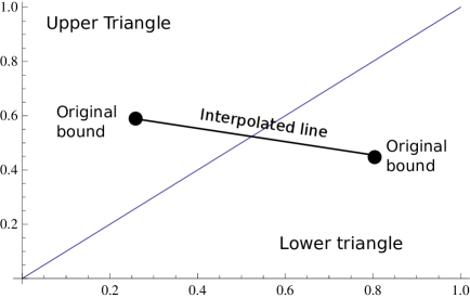
Figure 1.4: A Riesz diagram

The interpolation theorem was originally stated by M. Riesz in [Rie27b]. In the paper, the theorem was stated only for the lower triangle in the Riesz diagram, i.e., for $p_{n}\leq q_{n}$. Since the proof of the theorem made use of convexity results for bilinear forms, the interpolation theorem is often referred to as the Riesz convexity theorem. The extension of the theorem to the entire square is due to O. Thorin, originally published in his 1938 paper and explicated further in [Tho48]. The modern proof of the theorem was first provided by J. Tamarkin and A. Zygmund in [TZ44] and makes use of an extension of the maximum modulus principle from complex analysis:

Theorem 1.44 (Hadamard’s three-lines theorem).

Let $\Phi$ be a holomorphic function in the interior of the closed strip

$$S=\{z\in\mathbb{C}:0\leq\operatorname{Re}z\leq 1\}$$

and bounded and continuous on $S$. If $|\Phi(z)|\leq k_{0}$ on the line $\operatorname{Im}z=0$ and $|\Phi(z)|\leq k_{1}$ on the line $\operatorname{Im}z=1$, then, for each $0\leq\theta\leq 1$, we have the inequality

$$|\Phi(z)|\leq k_{0}^{1-\theta}k_{1}^{\theta}$$

on the line $\operatorname{Im}z=\theta$.

Proof.

We define holomorphic functions

$$\Psi(z)=\frac{\Phi(z)}{k_{0}^{1-z}k_{1}^{z}}\hskip 14.45377pt\mbox{and}\hskip 14.45377pt\Psi_{n}(z)=\Psi(z)e^{(z^{2}-1)/n},$$

so that $\Psi_{n}\to\Psi$ as $n\to\infty$. We wish to show that $|\Psi(z)|\leq 1$ on $S$.

To this end, we first note that $|\Psi(z)|\leq 1$ on the lines $\operatorname{Im}z=0$ and $\operatorname{Im}z=1$. Moreover, $\Phi$ is bounded above on $S$, and $k_{0}^{1-z}k_{1}^{z}$ is bounded below on $S$, hence we have the bound $|\Psi(z)|\leq M$ on $S$. Noting the inequality

$$|\Psi_{n}(x+iy)|\leq Me^{-y^{2}/n}e^{(x^{2}-1)/n}\leq Me^{-y^{2}/n},$$

we see that $\Psi_{n}(x+iy)$ converges uniformly to 0 as $|y|\to\infty$. We can therefore find $y_{n}>0$ such that $|\Psi_{n}(x+iy)|\leq 1$ for all $|y|\geq y_{n}$ and $0\leq x\leq 1$, whence by the maximum modulus principle we have $|\Psi_{n}(z)|\leq 1$ on the rectangle

$$\{z=x+iy:0\leq x\leq 1\mbox{ and }-y_{n}\leq y\leq y_{n}\}.$$

It follows that $|\Psi_{n}(z)|\leq 1$ on $S$ for each $n\in\mathbb{N}$, and sending $n\to\infty$ yields the desired result. ∎

We now come to the proof of the interpolation theorem. In the words of C. Fefferman in [Fef95], the proof essentially amounts to providing an estimate for the integral

$$\int_{Y}(Tf)g\,d\nu,$$

where $f\in L^{p_{\theta}}(X,\mu)$ and $g\in L^{q_{\theta}^{\prime}}(Y,\nu)$. In light of the Riesz representation theorem, the supremum of the above expression equals $\|Tf\|_{q_{\theta}}$. To give an upper bound for the above integral, we begin by finding nonnegative real numbers $F$ and $G$ and real numbers $\phi$ and $\psi$ such that $f=Fe^{i\phi}$ and $g=Ge^{i\psi}$, and consider the entire function

$$\Phi(z)=\int_{Y}(Tf_{z})g_{z}\,d\nu,$$

where $f_{z}=F^{az+b}e^{i\phi}$ and $g_{z}=G^{cz+d}e^{i\psi}$ for suitably chosen real numbers $a,b,c,d$. We pick $a,b,c,d$ such that

$$|f_{z}|^{p_{0}}=|f|^{p_{\theta}}\hskip 14.45377pt\mbox{and}\hskip 14.45377pt|g_{z}|^{q_{0}^{\prime}}=|g|^{q_{\theta}^{\prime}}$$

on the line $\operatorname{Re}z=0$,

$$|f_{z}|^{p_{1}}=|f|^{p_{\theta}}\hskip 14.45377pt\mbox{and}\hskip 14.45377pt|g_{z}|^{q_{1}^{\prime}}=|g|^{q_{\theta}^{\prime}}$$

on the line $\operatorname{Re}z=1$, and

$$f_{z}=f\hskip 14.45377pt\mbox{ and }\hskip 14.45377ptg_{z}=g$$

at the point $z=\theta$.

The first assumption yields an upper bound $k_{0}^{\prime}$ for both $\|f_{z}\|_{p_{0}}$ and $\|g_{z}\|_{q_{0}^{\prime}}$ on the line $\operatorname{Re}z=1$, and so the $L^{p_{0}}\to L^{q_{0}}$ norm inequality of $T$ yields the estimate

$$|\Phi(z)|\leq k_{0}$$

on the line $\operatorname{Re}z=0$ for some constant $k_{0}$. Similarly, the second assumption furnishes a constant $k_{1}$ such that

$$|\Phi(z)|\leq k_{1}$$

on the line $\operatorname{Re}z=1$. By Hadamard’s three-lines theorem, we now have the bound $|\Phi(z)|\leq k_{0}^{1-\theta}k_{1}^{\theta}$, and the third assumption implies that

$$\left|\int_{Y}(Tf)g\,d\nu\right|\leq k_{0}^{1-\theta}k_{1}^{\theta}.$$

We now present the proof in full detail.

Proof of Theorem 1.43.

Fix $0\leq\theta\leq 1$. For notational convenience, we let

$$\alpha_{0}=\frac{1}{p_{0}},\hskip 7.22743pt\alpha_{1}=\frac{1}{p_{1}},\hskip 7.22743pt\alpha=\frac{1}{p_{\theta}},\hskip 7.22743pt\beta_{0}=\frac{1}{q_{0}},\hskip 7.22743pt\beta_{1}=\frac{1}{q_{1}},\hskip 7.22743pt\beta=\frac{1}{q_{\theta}}.$$

With this notation, we set

$$\alpha(z)=(1-z)\alpha_{0}+z\alpha_{1}\hskip 14.45377pt\mbox{and}\hskip 14.45377pt\beta(z)=(1-z)\beta_{0}+z\beta_{1},$$

so that

$$\alpha(0)=\alpha_{0},\hskip 7.22743pt\alpha(1)=\alpha_{1},\hskip 7.22743pt\alpha(\theta)=\alpha,\hskip 7.22743pt\beta(0)=\beta_{0},\hskip 7.22743pt\beta(1)=\beta_{1},\hskip 7.22743pt\beta(\theta)=\beta.$$

We shall first prove the theorem for simple functions with finite-measure support, which evidently belong to $D\cap L^{p_{\theta}}(X,\mu)$. By the Riesz representation theorem, we have

$$\|Tf\|_{q_{\theta}}=\sup\left|\int_{Y}(Tf)g\,d\nu\right|$$

for each simple function $f$, where the supremum is taken over all simple functions $g$ of $L^{q_{\theta}^{\prime}}$-norm at most one. Therefore, it suffices to show that

$$\left|\int_{Y}(Tf)g\,d\nu\right|\leq k_{0}^{1-\theta}k_{1}^{\theta}\|f\|_{p_{\theta}}$$

for each such $g$. If $\|f\|_{p_{\theta}}=0$, then there is nothing to prove, and so we can assume by renormalization of $f$ that $\|f\|_{p_{\theta}}=1$. We thus set out to establish

$$\left|\int_{Y}(Tf)g\,d\nu\right|\leq k_{0}^{1-\theta}k_{1}^{\theta}$$

for all simple functions $g$ with $\|g\|_{q_{\theta}^{\prime}}=1$.

We now suppose that

$$f=\sum_{j=1}^{m}a_{j}\chi_{E_{j}}\hskip 14.45377pt\mbox{ and }\hskip 14.45377ptg=\sum_{k=1}^{n}b_{k}\chi_{F_{k}}$$

are two simple functions satisfying the above conditions. We also assume without loss of generality that $p_{\theta}<\infty$ and $q_{\theta}>1$, so that $\alpha>0$ and $\beta<1$. Write $a_{j}=|a_{j}|e^{i\theta_{j}}$ and $b_{k}=|b_{k}|e^{i\varphi_{k}}$ and set

$$f_{z}=\sum_{j=1}^{m}|a_{j}|^{\alpha(z)/\alpha}e^{i\theta_{j}}\chi_{E_{j}}\hskip 14.45377pt\mbox{and}\hskip 14.45377ptg_{z}=\sum_{k=1}^{m}|b_{k}|^{(1-\beta(z))/(1-\beta)}e^{i\varphi_{k}}\chi_{F_{k}}$$

for each $z\in\mathbb{C}$. Then

$$\Phi(z)=\int_{Y}(Tf_{z})g_{z}\,d\nu$$

is an entire function such that

$$\Phi(\theta)=\int_{Y}(Tf)g\,d\nu.$$

We note, in particular, that $\Phi$ is holomorphic in the interior of $S$ and is continuous on $S$. Since $T$ is linear, we see that

$$\Phi(z)=\sum_{j=1}^{m}\sum_{k=1}^{n}|a_{j}|^{\alpha(z)/\alpha}|b_{k}|^{(1-\beta(z))/(1-\beta)}\left(e^{i(\theta_{j}+\varphi_{k})}\int_{Y}(T\chi_{E_{j}})\chi_{F_{k}}\right),$$

whence $F$ is bounded on $S$.

We now furnish a bound for $\Phi$ on the lines $\operatorname{Re}z=0$ and $\operatorname{Re}z=1$. Note first that $|\Phi(z)|\leq\|Tf_{z}\|_{q_{0}}\|g_{z}\|_{q_{\theta}^{\prime}}$ by Hölder’s inequality. Observing the identities $\alpha(z)=\alpha_{0}+z(\alpha_{1}-\alpha_{0})$ and $1-\beta(z)=(1-\beta_{0})-z(\beta_{1}-\beta_{0})$ on the line $\operatorname{Re}z=0$, we see that

$$|f_{z}|^{p_{0}} = |e^{i\arg f}|f|^{z(\alpha_{1}-\alpha_{0})/\alpha}|f|^{p_{\theta}/p_{0}}|^{p_{0}}=|f|^{p_{\theta}}$$

$$|g_{z}|^{q_{0}^{\prime}} = |e^{i\arg g}|g|^{-z(\beta_{1}-\beta_{0})/(1-\beta)}|g|^{q_{\theta}^{\prime}/q_{0}^{\prime}}|^{q_{0}^{\prime}}=|g|^{q_{\theta}^{\prime}}.$$

Since $T$ is of type $(p_{0},q_{0})$, it thus follows that

$$|\Phi(z)| \leq \|Tf_{z}\|_{q_{0}}\|g_{z}\|_{q_{\theta}^{\prime}}$$

$$\leq k_{0}\|f_{z}\|_{p_{0}}\|g_{z}\|_{q_{0}^{\prime}}$$

$$= k_{0}\left(\int_{X}|f|^{p}\,d\mu\right)^{1/p_{0}}\left(\int_{Y}|g|^{q_{0}^{\prime}}\,d\nu\right)^{1/q_{0}}$$

$$\leq k_{0}\|f\|_{p}^{p_{\theta}/p_{0}}\|g\|_{q}^{q_{\theta}^{\prime}/q_{0}^{\prime}}$$

$$\leq k_{0}$$

on the line $\operatorname{Re}z=0$. A similar computation establishes the bound $|\Phi(z)|\leq k_{1}$ on the line $\operatorname{Re}z=1$, whence by Hadamard’s three-lines theorem we have the inequality

$$|\Phi(z)|\leq k_{0}^{1-\theta}k_{1}^{\theta}$$

on the line $\operatorname{Re}z=\theta$. Setting $z=\theta$, we have

$$\left|\int_{Y}(Tf)g\,d\nu\right|=|\Phi(\theta)|\leq k_{0}^{1-\theta}k_{1}^{\theta},$$

which is the desired inequality.

Having established the theorem for simple functions, we now prove the theorem for the general function $f\in D\cap L^{p}(X,\mu)$. To this end, we shall furnish a sequence $(f_{n})_{n=1}^{\infty}$ of simple functions such that

$$\lim_{n\to\infty}\|f_{n}-f\|_{p_{\theta}}=0\hskip 14.45377pt\mbox{and}\hskip 14.45377pt\lim_{n\to\infty}(Tf_{n})(x)=(Tf)(x),$$

for then Fatou’s lemma yields the inequality

$$\|Tf\|_{q_{\theta}}\leq\lim_{n\to\infty}\|Tf_{n}\|_{q_{\theta}}\leq\lim_{n\to\infty}k_{0}^{1-\theta}k_{1}^{\theta}\|f_{n}\|_{p_{\theta}}=k_{0}^{1-\theta}k_{1}^{\theta}\|f\|_{p_{\theta}}.$$

Therefore, the task of proving the theorem reduces to finding such a sequence.

We assume without loss of generality that $f\geq 0$ and $p_{0}\leq p_{1}$. Let $f^{0}$ be the truncation of $f$, defined as

$$f^{0}(x)=\begin{cases}f(x)&\mbox{ if }f(x)>1;\\ 0&\mbox{ if }f(x)\leq 1;\end{cases}$$

and $f^{1}=f-f^{0}$ another truncation. $D$ contains all truncations of $f$, and $(f^{0})^{p_{0}}$ and $(f^{1})^{p_{1}}$ are bounded by $f^{p}$, hence $f^{0}\in D\cap L^{p_{0}}(X,\mu)$ and $f^{1}\in D\cap L^{p_{1}}(X,\mu)$. We can find a monotonically increasing sequence $(g_{m})_{m=1}^{\infty}$ converging to $f$, which satisfies

$$\lim_{m\to\infty}\|g_{m}-f\|_{p_{\theta}}=0$$

by the monotone convergence theorem. If $g_{m}^{0}$ and $g_{m}^{1}$ are truncations of $g_{m}$ defined in the same way as $f^{0}$ and $f^{1}$, then we have

$$\lim_{m\to\infty}\|g_{m}^{0}-f^{0}\|_{p_{\theta}}=\lim_{m\to\infty}\|g_{m}^{1}f^{1}\|_{p_{\theta}}=0.$$

Since $T$ is of types $(p_{0},q_{0})$ and $(p_{1},q_{1})$, we have

$$\lim_{m\to\infty}\|Tg_{m}^{0}-Tf^{0}\|_{q_{0}}=\lim_{m\to\infty}\|Tg_{m}^{1}-Tf^{1}\|_{q_{1}}=0.$$

We can then find a subsequence of $(Tg_{m}^{0})_{m=1}^{\infty}$ converging almost everywhere to $Tf^{0}$, whence we may as well assume that the full sequence converges almost everywhere to $Tf^{0}$. Similarly, we can find a subsequence $(g_{m_{n}})_{n=1}^{\infty}$ of $(g_{m})_{m=1}^{\infty}$ such that $(Tg_{m_{n}}^{1})_{n=1}^{\infty}$ converges almost everywhere to $Tf^{1}$, whence the sequence $(f_{n})_{n=1}^{\infty}$ defined by setting

$$f_{n}=g_{m_{n}}^{0}+g_{m_{n}}^{1}$$

is the desired sequence. This completes the proof of the Riesz-Thorin interpolation theorem. ∎

1.4.2 Corollaries of the Interpolation Theorem

We now recall the Hausdorff-Young inequality from the last section:

Theorem 1.45 (Hausdorff-Young inequality).

For each $1\leq p\leq 2$, the $L^{p}$ Fourier transform is a bounded linear operator from $L^{p}(\mathbb{R}^{d})$ into $L^{p^{\prime}}(\mathbb{R}^{d})$. Specifically, we have the inequality

$$\|\hat{f}\|_{p^{\prime}}\leq\|f\|_{p},$$

whence the $L^{p}\to L^{p^{\prime}}$ operator norm of $\mathscr{F}$ is at most 1.

The inequality is now a trivial consequence of the interpolation theorem, for the Fourier transform is a bounded operator from $L^{1}$ into $L^{\infty}$ and from $L^{2}$ into $L^{2}$, whose operator norm is at most 1 in both cases.

Another application is the following generalization of Young’s inequality:

Theorem 1.46 (Young’s inequality).

If $1\leq p,q,r\leq\infty$ such that

$$\frac{1}{p}+\frac{1}{q}=1+\frac{1}{r},$$

then

$$\|f*g\|_{r}\leq\|f\|_{p}\|g\|_{q}$$

for all $f\in L^{p}(\mathbb{R}^{d})$ and $g\in L^{q}(\mathbb{R}^{d})$.

Again, the proof is a routine application of the interpolation theorem on the convolution operator

$$Tg=f*g,$$

once we recall the Young’s inequality to establish that $T$ is of type $(1,p)$ and invoke the bound

$$\|f*g\|_{\infty}\leq\|f\|_{p}\|g\|_{p^{\prime}}$$

from Theorem 1.26 to prove that $T$ is of type $(p^{\prime},\infty)$. We shall have more to say about convolution operators in §2.3. The constants in the above inequalities can be improved: see §§1.5.8 for the sharp versions.

1.4.3 The Stein Interpolation Theorem

Let $(X,\mathfrak{M},\mu)$ and $(Y,\mathfrak{N},\nu)$ be $\sigma$-finite measure spaces and $T$ a linear operator of types $(p_{0},q_{0})$ and $(p_{1},q_{1})$. Recall that the proof of the Riesz-Thorin interpolation theorem essentially amounted to giving an estimate of the entire function

$$z\mapsto\int_{Y}(Tf_{z})g_{z}\,d\nu$$

What if we let the operator $T$ vary as well? C. Fefferman points out in [Fef95] that the net result of adding a letter $z$ to the operator $T$ is the new entire function

$$\Phi(z)=\int_{Y}(T_{z}f_{z})g_{z}\,d\nu,$$

whence establishing an estimate of $\Phi$ produces another interpolation theorem. The similarity of the operators suggest that the new proof should closely mimic that of the Riesz-Thorin interpolation theorem, and this is indeed the case.

We thus obtain an interpolation theorem that allows the operator to vary in a holomorphic manner, as the letter $z$ suggests. The interpolation theorem was first established by E. Stein in [Ste56] and is dubbed interpolation of analytic families of operators in the standard reference [SW71] of E. Stein and G. Weiss. In the present thesis, we shall refer to it as the Stein interpolation theorem.

In order for $\Phi$ to be holomorphic, we must impose a restriction on how the operator can vary:

Definition 1.47.

Let $(X,\mathfrak{M},\mu)$ and $(Y,\mathfrak{N},\nu)$ be $\sigma$-finite measure spaces and

$$S=\{z\in\mathbb{C}:0\leq\operatorname{Re}z\leq 1\}.$$

We suppose that we are given a linear operator $T_{z}$, for each $z\in S$, on the space of simple functions in $L^{1}(M,\mu)$ into the space of measurable functions on $N$. If $f$ is a simple function in $L^{1}(M,\mu)$ and $g$ a simple function in $L^{1}(N,\nu)$, we assume furthermore that $(T_{z}f)g\in L^{1}(N,\nu)$. The family $\{T_{z}\}_{z\in S}$ of operators is said to be admissible if, for each such $f$ and $g$, the map

$$z\mapsto\int_{N}(T_{z}f)g\,d\nu$$

is holomorphic in the interior of $S$ and continuous on $S$, and if there exists a constant $k<\pi$ such that

$$\sup_{z\in S}e^{-k|\operatorname{Im}z|}\left|\int_{N}(T_{z}f)g\,d\nu\right|<\infty.$$

With this hypothesis, we can state the interpolation theorem as follows:

Theorem 1.48 (Stein interpolation theorem).

Let $(X,\mathfrak{M},\mu)$ and $(Y,\mathfrak{N},\nu)$ be $\sigma$-finite measure spaces and $\{T_{z}\}_{z\in S}$ an admissible family of linear operators. Fix $1\leq p_{0},p_{1},q_{0},q_{1}\leq\infty$ and assume, for each real number $y$, that there are constants $M_{0}(y)$ and $M_{1}(y)$ such that

$$\|T_{iy}f\|_{q_{0}}\leq M_{0}(y)\|f\|_{p_{0}}\hskip 14.45377pt\mbox{and}\hskip 14.45377pt\|T_{1+iy}f\|_{q_{1}}\leq M_{1}(y)\|f\|_{p_{1}}$$

for each simple function $f$ in $L^{1}(M,\mu)$. If, in addition, the constants $M_{j}(y)$ satisfy

$$\sup_{-\infty<y<\infty}e^{-k|y|}\log M_{j}(y)<\infty$$

for some $k<\pi$, then each $\theta\in[0,1]$ furnishes a constant $M_{\theta}$ such that

$$\|T_{\theta}f\|_{q_{\theta}}\leq M_{\theta}\|f\|_{p_{\theta}}$$

for each simple function $f$ in $L^{1}(M,\mu)$, where

$$p_{\theta}^{-1} = (1-\theta)p_{0}^{-1}+\theta p_{1}^{-1};$$

$$q_{\theta}^{-1} = (1-\theta)q_{0}^{-1}+\theta q_{1}^{-1}.$$

Theorem 1.11 then implies that $T_{\theta}$ can be extended to a bounded operator on $L^{p_{\theta}}(\mathbb{R}^{d})$ into $L^{q_{\theta}}(\mathbb{R}^{d})$. For the sake of convenience, we shall use the term operator of type $(p_{\theta},q_{\theta})$ for $T_{\theta}$ as well. The proof of the interpolation theorem makes use of an extension of Hadamard’s three-lines theorem due to I. Hirschman:

Lemma 1.49 (Hirschman).

If $\Phi$ is a continuous function on the strip $S$ that is holomorphic in the interior of $S$ and satisfies the bound

$$\sup_{z\in S}e^{-k|\operatorname{Im}z|}\log|\Phi(z)|<\infty$$ (1.10)

for some constant $k<\pi$, then

$$\log|\Phi(\theta)|\leq\frac{\sin\pi\theta}{2}\int_{-\infty}^{\infty}\frac{\log|\Phi(iy)|}{\cosh\pi y-\cos\pi\theta}+\frac{\log|\Phi(1+iy)|}{\cosh\pi y+\cos\pi\theta}\,dy$$ (1.11)

for all $\theta\in(0,1)$.

Why is this an extension of Hadamard’s three-lines theorem? If $\Phi$ is bounded and continuous on $S$, $|\Phi(z)|\leq k_{0}$ on the line $\operatorname{Im}z=0$ and $|\Phi(z)|\leq k_{1}$ on the line $\operatorname{Im}z=1$, then the bound

$$\sup_{z\in S}e^{-k|\operatorname{Im}z|}\log|\Phi(z)|<\infty$$

is satisfied for $k=0$. Furthermore, we have

$$\frac{1}{2}\int_{-\infty}^{\infty}\frac{\log|\Phi(iy)|}{\cosh\pi y-\cos\pi\theta}\,dy=\theta\hskip 14.45377pt\mbox{and}\hskip 14.45377pt\frac{1}{2}\int_{-\infty}^{\infty}\frac{\log|\Phi(1+iy)|}{\cosh\pi y+\cos\pi\theta}\,dy=1-\theta,$$

whence Hirschman’s lemma implies that

$$|\Phi(x)|\leq k_{0}^{1-\theta}k_{1}^{\theta}.$$

We have thus recovered the three-lines theorem from Hirschman’s lemma.

Proof of Lemma 1.49.

Let $D$ be the closed unit disk in $\mathbb{C}$. For each $\zeta$ in $D\smallsetminus\{-1,1\}$, we define

$$\varphi(\zeta)=\frac{1}{\pi i}\log\left(i\frac{1+\zeta}{1-\zeta}\right).$$

$\varphi$ is a composition of the conformal mapping

$$\zeta\mapsto w=i\frac{1+\zeta}{1-\zeta}$$

of $D\smallsetminus\{-1,1\}$ onto the closed upper-half plane $\mathbb{H}$ and of the conformal mapping

$$w\mapsto z=\frac{1}{\pi i}\log w$$

of $\mathbb{H}$ onto the closed strip $S$. Therefore, $h$ maps $D\smallsetminus\{-1,1\}$ conformally onto $S$, and the inverse

$$\zeta=\varphi^{-1}(z)=\frac{e^{\pi iz}-i}{e^{\pi iz}+i}$$

is conformal as well. $\Psi=\Phi\circ\varphi$ is holomorphic on open unit disk and is continuous on $D\smallsetminus\{-1,1\}$.

We now recall the following standard result from complex analysis:

Lemma 1.50 (Poisson-Jensen formula).

Let $\Psi$ be a holomorphic function on an open disk of radius $R$ centered at 0. If, for some $0<\rho<R$, we write $a_{1},\ldots,a_{N}$ to denote the zeroes of $\Psi$ in the open disk $|z|<\rho$, then

$$\log|\Psi(z)|=-\sum_{n=1}^{N}\log\left|\frac{\rho^{2}-\bar{a}_{n}z}{\rho(z-a_{n})}\right|+\frac{1}{2\pi}\int_{0}^{2\pi}\operatorname{Re}\frac{\rho e^{i\theta}+z}{\rho e^{i\theta}-z}\log|f(\rho e^{i\theta})|\,d\theta$$

for all $|z|<r$ such that $f(z)\neq 0$.

For $0\leq\rho<R<1$, we can write $\zeta=\rho e^{i\omega}$ and apply the above lemma to obtain

$$\log|\Psi(\zeta)|\leq\frac{1}{2\pi}\int_{-\pi}^{\pi}\frac{R^{2}-\rho^{2}}{R^{2}-2R\rho\cos(\omega-\phi)+\rho^{2}}\log|\psi(Re^{i\phi})|\,d\phi.$$ (1.12)

Rewriting (1.10) in terms of $\Psi$ and $\eta=\varphi^{-1}(x+iy)$, we have

$$\log|\Psi(\eta)|\leq C\left[|1+\eta|^{-k/\pi}+|1-\eta|^{-k/\pi}\right]$$

for some constant $C$ independent of $\eta\in D$. Plugging in $\eta=Re^{i\phi}$ and noting that $k/\pi<1$, we see that the above inequality permits us to use the dominated convergence theorem to the integral in (1.12). Therefore, by sending $R\to 1$, we obtain

$$\log|\Psi(\zeta)|\leq\frac{1}{2\pi}\int_{-\pi}^{\pi}\frac{1-\rho^{2}}{1-2\rho\cos(\omega-\phi)+\rho^{2}}\log|\psi(e^{i\phi})|\,d\phi.$$ (1.13)

We now apply a change of variables to (1.13) inequality to obtain (1.11). First, we convert the condition

$$0<\omega=\varphi(\rho e^{i\omega})<1$$ (1.14)

into a condition on $\rho$ and $\omega$. Indeed, we note that

$$\rho e^{i\omega}=\varphi^{-1}(\theta)=\frac{e^{\pi i\theta}-i}{e^{\pi i\theta}+i}=-i\frac{\cos\pi\theta}{1+\sin\pi\theta}=\left(\frac{\cos\pi\theta}{1+\sin\pi\theta}\right)e^{i\pi/2},$$

whence (1.14) implies that

$$\rho=\begin{cases}\frac{\cos\pi\theta}{1+\sin\pi\theta}&\mbox{ if }0<\theta\leq\frac{1}{2};\\ -\frac{\cos\pi\theta}{1+\sin\pi\theta}&\mbox{ if }\frac{1}{2}\leq\theta<1;\end{cases}\hskip 14.45377pt\mbox{and}\hskip 14.45377pt\omega=\begin{cases}-\frac{\pi}{2}&\mbox{ if }0<\theta\leq\frac{1}{2};\\ \frac{\pi}{2}&\mbox{ if }\frac{1}{2}\leq\theta<1.\end{cases}$$

Therefore, if $0<\theta\leq\frac{1}{2}$, then

$$\frac{1-\rho^{2}}{1-2\rho\cos(\omega-\phi)+\rho^{2}} = \frac{1-\rho^{2}}{1-2\rho\cos(\phi+\pi/2)+\rho^{2}}$$

$$= \frac{1-\rho^{2}}{1+2\rho\sin\phi+\rho^{2}}$$

$$= \frac{\sin\pi\theta}{1+\cos\pi\theta\sin\phi}.$$

Furthermore, the above equality holds for $\frac{1}{2}\leq\theta<1$ as well.

We now observe from the identity

$$e^{i\phi}=\varphi^{-1}(iy)=\frac{e^{-\pi y}}{e^{-\pi y}+i}$$

that $y$ ranges from $+\infty$ to $-\infty$ as $\phi$ ranges from $-\pi$ to $0$. Moreover,

$$\sin\phi=-\frac{1}{\cosh\pi y}\hskip 14.45377pt\mbox{and}\hskip 14.45377ptd\phi=-\frac{\pi}{\cosh\pi y}dy,$$

and so the change-of-variables formula yields

$$\frac{1}{2\pi}\int_{-\pi}^{0}\frac{1-\rho^{2}}{1-2\rho\cos(\omega-\phi)+\rho^{2}}\log|\Psi(e^{i\phi})|\,d\phi$$

$$= \frac{\sin\pi\theta}{2}\int_{-\infty}^{\infty}\frac{\log|\Phi(iy)|}{\cosh\pi y-\cos\pi\theta}\,dy.$$

Similarly, as $\phi$ ranges from $0$ to $\pi$, the function $\varphi(e^{\phi})$ produces the points $1+iy$ with $-\infty<y<\infty$, whence

$$\frac{1}{2\pi}\int_{0}^{\pi}\frac{1-\rho^{2}}{1-2\rho\cos(\omega-\phi)+\rho^{2}}\log|\Psi(e^{i\phi})|\,d\phi$$

$$= \frac{\sin\pi\theta}{2}\int_{-\infty}^{\infty}\frac{\log|\Phi(1+iy)|}{\cosh\pi y+\cos\pi\theta}\,dy.$$

We add up the two quantities and plug the sum into (1.13) to obtain (1.11), which was the desired inequality. ∎

We are now ready to present a proof of the interpolation theorem.

Proof of Theorem 1.48.

Fix $0\leq\theta\leq 1$. As in the proof of the Riesz-Thorin interpolation theorem, we let

$$\alpha_{0}=\frac{1}{p_{0}},\hskip 7.22743pt\alpha_{1}=\frac{1}{p_{1}},\hskip 7.22743pt\alpha=\frac{1}{p_{\theta}},\hskip 7.22743pt\beta_{0}=\frac{1}{q_{0}},\hskip 7.22743pt\beta_{1}=\frac{1}{q_{1}},\hskip 7.22743pt\beta=\frac{1}{q_{\theta}}.$$

With this notation, we set

$$\alpha(z)=(1-z)\alpha_{0}+z\alpha_{1}\hskip 14.45377pt\mbox{and}\hskip 14.45377pt\beta(z)=(1-z)\beta_{0}+z\beta_{1},$$

so that

$$\alpha(0)=\alpha_{0},\hskip 7.22743pt\alpha(1)=\alpha_{1},\hskip 7.22743pt\alpha(\theta)=\alpha,\hskip 7.22743pt\beta(0)=\beta_{0},\hskip 7.22743pt\beta(1)=\beta_{1},\hskip 7.22743pt\beta(\theta)=\beta.$$

Let

$$f=\sum_{j=1}^{m}a_{j}\chi_{E_{j}}\hskip 14.45377pt\mbox{ and }\hskip 14.45377ptg=\sum_{k=1}^{n}b_{k}\chi_{F_{k}}$$

be simple functions such that $f\in L^{1}(X,\mu)$, $g\in L^{1}(Y,\nu)$, and

$$\|f\|_{p_{\theta}}=1=\|g\|_{q_{\theta}^{\prime}}.$$

Write $a_{j}=|a_{j}|e^{i\theta_{j}}$ and $b_{k}=|b_{k}|e^{i\varphi_{k}}$ and set

$$f_{z}=\sum_{j=1}^{m}|a_{j}|^{\alpha(z)/\alpha}e^{i\theta_{j}}\chi_{E_{j}}\hskip 14.45377pt\mbox{and}\hskip 14.45377ptg_{z}=\sum_{k=1}^{m}|b_{k}|^{(1-\beta(z))/(1-\beta)}e^{i\varphi_{k}}\chi_{F_{k}}$$

for each $z\in\mathbb{C}$. Then

$$\Phi(z)=\int_{Y}(T_{z}f_{z})g_{z}\,d\nu$$

is an entire function such that

$$\Phi(\theta)=\int_{Y}(T_{\theta}f)g\,d\nu.$$

We note, in particular, that $\Phi$ is holomorphic in the interior of $S$ and is continuous on $S$. Since $T_{z}$ is linear, we see that

$$\Phi(z)=\sum_{j=1}^{m}\sum_{k=1}^{n}|a_{j}|^{\alpha(z)/\alpha}|b_{k}|^{(1-\beta(z))/(1-\beta)}\left(e^{i(\theta_{j}+\varphi_{k})}\int_{Y}(T_{z}\chi_{E_{j}})\chi_{F_{k}}\right).$$

It follows that $\{T_{z}\}_{z\in S}$ is an admissible family, whence $\Phi$ satisfies the bound

$$\sup_{z\in S}e^{-k|\operatorname{Im}z|}\log|\Phi(z)|<\infty.$$

Furthermore, we have

$$|f_{iy}|^{p_{0}}=|f|^{p_{\theta}}=|f_{1+iy}|^{p_{1}}\hskip 14.45377pt\mbox{and}\hskip 14.45377pt|g_{iy}|^{q_{0}^{\prime}}=|g|^{q_{\theta}^{\prime}}=|g_{1+iy}|^{q_{1}^{\prime}}$$

for all $y\in\mathbb{R}$, and so Hölder’s inequality implies that $|\Phi(iy)|\leq M_{0}(y)$ and $|\Phi(1+iy)|\leq M_{1}(y)$. Hirschman’s lemma now establishes the bound

$$|\Phi(\theta)|$$

$$\leq \exp\left(\frac{\sin(\pi\theta)}{2}\int_{-\infty}^{\infty}\frac{\log|\Phi(iy)|}{\cosh\pi y-\cos\pi\theta}+\frac{\log|\Phi(1+iy)|}{\cosh\pi y+\cos\pi\theta}\,dy\right)$$

$$= M_{\theta},$$

whence we invoke the Riesz representation theorem to conclude that

$$\|T_{\theta}f\|_{q_{\theta}}=\sup_{\|g\|_{q_{\theta}^{\prime}}=1}\left|\int_{Y}(T_{\theta}f)g\,d\nu\right|\leq M_{\theta}=M_{\theta}\|f\|_{p_{\theta}},$$

as was to be shown. ∎

See §§2.7.6 for an application of the Stein interpolation theorem in the context of the Fourier inversion problem. In §2.5, we shall prove Fefferman’s generalization of the Stein interpolation theorem that allows us to take a particular subspace of $L^{1}$ as the domain for one of the endpoint estimates. The theory of complex interpolation, which provides an abstract framework for Riesz-Thorin, Stein, and Fefferman-Stein, will be developed in §2.2.

1.5 Additional Remarks and Further Results

In this section, we collect miscellaneous comments that provide further insights or extension of the material discussed in the chapter. No result in the main body of the thesis relies on the material presented herein.

1.5.1.

If $X$ is a topological space, then a compactification of $X$ is defined to be a compact Hausdorff space $Y$ such that $X$ embeds into $Y$ as a dense subset of $Y$. The extended real line $\bar{\mathbb{R}}$ can be considered as a compactification of $\mathbb{R}$, if, in addition to the open sets in $\mathbb{R}$, we declare the intervals of the form $[-\infty,a)$ and $(a,\infty]$ as open sets in $\bar{\mathbb{R}}$. With this topology, an extended real-valued function $f$ is measurable if and only if $f^{-1}(U)$ is measurable for every open set $U$ in $\bar{\mathbb{R}}$, thus conforming to the standard definition of measurability.

1.5.2.

For $1<p<\infty$, the Riesz representation theorem continues to hold on non-$\sigma$-finite measure spaces: see Theorem 6.15 in [Fol99]. It thus follows that $L^{p}$ spaces for $1<p<\infty$ are always reflexive Banach spaces. As for $p=1$, the representation theorem continues to hold for a slightly milder condition that $\mu$ be decomposable: we say that $\mu$ is decomposable if there is a pairwise disjoint collection $\mathscr{F}$ of finite $\mu$-measure such that

1. The union of all members of $\mathscr{F}$ is the base set $X$;

2. If $E$ is of finite $\mu$-measure, then

   $$\mu(E)=\sum_{F\in\mathscr{F}}\mu(E\cap F);$$

3. If the intersection a subset $E$ of $X$ and each element of the collection $\mathscr{F}$ is $\mu$-measurable, then $E$ is $\mu$-measurable.

See Theorem 20.19 in [HS65] for a proof.

The dual of $L^{\infty}$ is strictly bigger than $L^{1}$, even on the Euclidean space. We define a bounded linear functional $l_{0}$ on $\mathcal{C}_{c}(\mathbb{R}^{d})$ by setting

$$l_{0}(f)=f(0)$$

for each $f\in\mathcal{C}_{c}(\mathbb{R}^{d})$. By Theorem 2.9, there exists a bounded extension $l$ of $l_{0}$ on $L^{\infty}(\mathbb{R}^{d})$. Assume for a contradiction that

$$l(f)=\int fu\,dx$$

for some $u\in L^{1}(\mathbb{R}^{d})$. Then $\int fu=0$ for all $f\in\mathcal{C}_{c}(\mathbb{R}^{d})$ such that $f(0)=0$, whence the discussion in §1.5.7 establishes that $u=0$ almost everywhere on $\mathbb{R}^{d}\smallsetminus\{0\}$. Therefore, $u=0$ almost everywhere on $\mathbb{R}^{d}$, and so

$$\int fu\,dx=0$$

for all $f\in L^{\infty}(\mathbb{R}^{d})$, which is evidently absurd.

In general, the dual of $L^{\infty}(X,\mathfrak{M},\mu)$ is isometrically isomorphic to the Banach space of finitely additive measures of bounded total variation that are absolutely continuous to $\mu$, which [DS58] denotes as $ba(X,\mathfrak{M},\mu_{1})$. See §IV.8.16 in [DS58] or §IV.9, Example 5 in [Yos80] for a proof of this representation theorem. Another “representation theorem” can be established if we consider $L^{\infty}$ as a $C^{*}$-algebra: see §12.20 in [Rud91].

1.5.3.

The Whitney decomposition theorem states that every nonempty closed set $F$ in $\mathbb{R}^{d}$ admits a countable collection $\{Q_{n}:n\in\mathbb{N}\}$ of almost-disjoint cubes such that the union of the cubes is $\mathbb{R}^{d}\smallsetminus F$ and

$$\operatorname{diam}Q_{n}\leq d(Q_{n},F)\leq 4\operatorname{diam}(Q_{n})$$

for each $n\in\mathbb{N}$. See §VI.1.2 in [Ste70] or Appendix J in [Gra08a] for a proof. Compare the decomposition theorem with the Calderón-Zygmund lemma: if $f$ is a nonnegative integrable function on $\mathbb{R}^{d}$ and $\alpha$ a positive constant, then there exists a decomposition $\mathbb{R}^{d}=F\cup\Omega$ such that

1. $F\cap\Omega=\varnothing$;

2. $f(x)\leq\alpha$ almost everywhere on $F$;

3. $\Omega$ is the union of almost-disjoint cubes $\{Q_{n}:n\in\mathbb{N}\}$ such that

   $$\alpha<\frac{1}{|Q_{n}|}\int_{Q_{n}}f(x)\,dx\leq 2^{d}\alpha.$$

This is of paramount importance in the theory of singular integrals, which we briefly touch upon in §2.4. A proof of the lemma can be found in [Ste70], I.3.3, although the lemma is usually integrated into the Calderón-Zygmund decomposition in many expositions: see Theorem 2.60 for details.

1.5.4.

Littlewood’s three principles serve as a useful guide for studying the properties of the Lebesgue measure. The first principle states that every set is nearly a finite sum of intervals. To make this precise, we recall that the symmetric difference of two sets $E$ and $F$ is defined by

$$E\Delta F=(E\smallsetminus F)\cup(F\smallsetminus E).$$

Proposition 1.51.

If $E\subseteq\mathbb{R}^{d}$ is of finite measure, then, for each $\varepsilon>0$, there exists a finite sequence $(Q_{n})_{n=1}^{N}$ of cubes such that

$$\left|E\Delta\bigcup_{n=1}^{N}Q_{n}\right|\leq\varepsilon.$$

The second principle, which states that every function is nearly continuous, can be stated as follows:

Theorem 1.52 (Lusin).

If $E$ is a finite-measure subset of $\mathbb{R}^{d}$ and $f:E\to\mathbb{C}$ a measurable function, then, for each $\varepsilon>0$, there exists a closed subset $F$ of $E$ such that $|E\smallsetminus F|\leq\varepsilon$ and $f|_{F}$ is continuous.

The third and the final principle states that every convergent sequence of functions is nearly uniformly convergent and can be formulated precisely as follows:

Theorem 1.53 (Egorov).

If $E$ is a finite-measure subset of $\mathbb{R}^{d}$ and $(f_{n})_{n=1}^{\infty}$ a sequence of measurable functions on $E$ that converge pointwise almost everywhere to $f:E\to\mathbb{C}$, then, for each $\varepsilon>0$, there exists a closed subset $F$ of $E$ such that $|E\smallsetminus F|\leq\varepsilon$ and $f_{n}\to f$ uniformly on $F$.

Lusin’s theorem can be established on more general domains, which can then be used to generalize Theorem 1.14. We shall take up on this matter in the next subsection.

1.5.5.

Theorem 1.14 can be generalized to locally compact Hausdorff domains with complete Borel regular measures. This is a direct consequence of the generalized Lusin’s theorem:

Theorem 1.54 (Lusin).

Let $\mu$ be a complete Borel regular measure on a locally compact Hausdorff space $X$. If $f$ is a complex-valued measurable function on $X$, $A$ a finite-measure subset of $X$, and $\operatorname{supp}f\subseteq A$, then each $\varepsilon>0$ admits a function $g\in\mathcal{C}_{c}(X)$ such that

$$\mu(\{x:f(x)\neq g(x)\})<\varepsilon\hskip 14.45377pt\mbox{and}\hskip 14.45377pt\sup_{x\in X}|g(x)|\leq\sup_{x\in X}|f(x)|.$$

See §2.24 in [Rud86] for a proof. Crucial in proving the above theorem is Urysohn’s lemma for locally compact Hausdorff spaces, which can be stated as follows:

Theorem 1.55 (Urysohn’s lemma).

Let $X$ be a locally compact Hausdorff space. For each open subset $O$ of $X$ and a compact subset $K$ of $O$, we can find a function $f\in\mathcal{C}_{c}(X)$ such that $0\leq f(x)\leq 1$ on $X$, $\operatorname{supp}f\subseteq O$, and $f(x)=1$ on $K$.

A proof of the above theorem can be found in [Rud86], §2.12. An even more general version of Lusin’s theorem for Radon measures appears in [Fol99] as Theorem 7.10. Urysohn’s lemma continues to hold for normal spaces: see §33 in [Mun00] or Theorem 4.15 in [Fol99] for a discussion.

1.5.6.

The name approximations to the identity (as in Theorem 1.23 and Corollary 1.24) can be motivated by considering a more abstract framework. A Banach algebra is a (complex) Banach space $\mathscr{A}$ with associative bilinear multiplication operation satisfying the inequality

$$\|xy\|\leq\|x\|\|y\|$$

for all $x,y\in\mathscr{A}$. Young’s inequality shows that the space $L^{1}$ equipped with the convolution operation is a Banach algebra.

Given a Banach algebra $\mathscr{A}$, a left approximate identity, or a left approximation to the identity, is a sequence $(e_{n})_{n=1}^{\infty}$ of elements in $\mathscr{A}$ such that

$$\lim_{n\to\infty}\|e_{n}x-x\|=0$$

for all $x\in\mathscr{A}$. While $e_{n}$ is not quite a multiplicative identity of the Banach algebra $\mathscr{A}$, it serves as one “at infinity”—hence the name “approximation to the identity”. Right approximate identities can be defined analogously.

1.5.7.

Another useful corollary of Theorem 1.23 is that, for $1\leq p<\infty$, an $L^{p}$ function $u$ on an open subset $O$ of $\mathbb{R}^{d}$ is zero almost everywhere on $\Omega$ in case

$$\int fu=0$$

for all $f\in\mathscr{C}_{c}^{\infty}$. See §1.5.2.

A consequence of the above result is that proving the equal almost-everywhere state of two functions amounts to integration the difference of two functions against a small class of “test functions”. This idea will be a recurring theme in distribution theory, which will be developed in §2.3.

1.5.8.

The optimal constant in the $d$-dimensional Hausdorff-Young inequality is $C_{p}^{d}$, where

$$C_{p}=\left(\frac{p^{1/p}}{(p^{\prime})^{1/p^{\prime}}}\right)^{1/2}.$$

The equality is achieved if and only if $f$ is of the form

$$f(x)=A\exp\left(-x\cdot Ax+b\cdot x\right),$$

where $A$ is a real symmetric positive-definite matrix and $b$ a vector in $\mathbb{C}^{n}$. The optimal constant was given for all $1\leq p\leq 2$ by William Beckner in [Bec75]. The necessary and sufficient condition for the equality, published in [Lie90], is due to Elliott Lieb.

The optimal constant for the $d$-dimensional generalized Young’s inequality, also established by Beckner in [Bec75], is $(C_{p}C_{q}C_{r^{\prime}})^{d}$, where the constants are defined as above. In [Lie90], Lieb gives a necessary and sufficient condition for an even more general version of Young’s inequality. See [LL01], Theorem 4.2 for a textbook exposition of the fully generalized Young’s inequality.

Chapter 2 The Modern Theory of Interpolation

The idea of the proof of the Riesz-Thorin interpolation theorem can be generalized to a class of operators on spaces other than the Lebesgue spaces. Alberto P. Calderón’s insight was to consider interpolation as an operation on spaces, rather than on operators. First published in [Cal64], Calderón’s complex method of interpolation absorbs the complex-analytic proof of the Riesz-Thorin interpolation theorem and provides an abstract framework in which many new interpolation theorems can be generated.

On the more concrete side, it became increasingly evident that many useful operators simply were not bounded on $L^{1}$ or $L^{\infty}$. Hardy spaces and the space of bounded mean oscillation were introduced as well-behaved substitutes, and it was proven by Charles Fefferman and Elias M. Stein in [FS72] that operators on these spaces can be interpolated as if they are on Lebesgue spaces. Precisely, the Fefferman-Stein interpolation theorem is a generalization of the Stein interpolation theorem on analytic families of operators, where the operator on $L^{1}$ can be bounded only on a subspace $H^{1}$ of $L^{1}$, and the operator on $L^{\infty}$ can satisfy a weaker estimate ($L^{\infty}\to\operatorname{BMO}$) than the usual estimate ($L^{\infty}\to L^{\infty}$).

The necessary machinery for these interpolation theorems is developed in the first and the third sections. In the fourth section, we study the Hilbert transform, which sets the stage for the Fefferman-Stein theory sketched in the fifth section. In the sixth and the last section, the Fefferman-Stein theory is applied to the study of differential equations and Fourier integral operators, and the complex interpolation method is applied to Sobolev spaces.

2.1 Elements of Functional Analysis

We begin the chapter by establishing a few key results from functional analysis, as explicated in many references such as [Bre11], [Lax02], [Rud91], [Yos80], and [DS58]. We have already encountered functional-analytic methods in Chapter 1, in which we often investigated the properties of spaces of functions rather than those of individual functions. We shall raise the level of abstraction even higher in this section, and study various kinds of topological vector spaces:

Definition 2.1.

A real or complex vector space $V$ is a topological vector space if $V$ is equipped with a topology such that the addition map $(x,y)\mapsto x+y$ and the scalar multiplication map $(a,v)\mapsto av$ are continuous.

2.1.1 Continuous Linear Functionals on Fréchet Spaces

$L^{p}$ spaces and, in general, Banach spaces are canonical examples of topological vector spaces. Some function spaces, however, do not admit one canonical norm. They might come with multiple natural norms; there might not be a convenient quotient construction to turn the norm-like map into a genuine norm. We are thus led to the following generalization:

Definition 2.2.

A seminorm on a topological vector space $V$ is a function $\rho:V\to[0,\infty)$ such that $\rho(av)=|a|v$ and $\rho(v+w)\leq\rho(v)+\rho(w)$ for all scalar $a$ and vectors $v$ and $w$.

We shall see in §2.3 that the canonical topology on $\mathscr{S}(\mathbb{R}^{d})$ is given by a countable collection of seminorms. This turns $\mathscr{S}(\mathbb{R}^{d})$ into a Fréchet space, which we now define.

Definition 2.3.

Let $V$ be a real or complex topological vector space. $V$ is a Fréchet space if $V$ is equipped with a countable collection $\{\rho_{n}:n\in\mathbb{N}\}$ of seminorms such that

$$d(v,w)=\sum_{n=1}^{\infty}\frac{1}{2^{n}}\left(\frac{\rho_{n}(v-w)}{1+\rho_{n}(v-w)}\right)$$

is a metric generating the topology of $V$.

We note that the seminorms $\rho_{n}$ are continuous in the topology defined as above. It is clear that every Banach space is a Fréchet space. While most function spaces we study in the present thesis are Banach spaces, we shall see that some are more naturally described in the language of Fréchet spaces.

For now, we study a different problem: namely, the existence of nontrivial continuous linear functionals. We know from linear algebra that finite-dimensional vector spaces have as many linear functionals as the vectors therein, and that each vector space is isomorphic to its dual space. It is not at all clear, however, if there are nonzero linear functionals on an infinite-dimensional space, let alone continuous ones.

There are, of course, some infinite-dimensional spaces with nontrivial continuous linear functionals. For example, we have seen that the $L^{p}$ spaces have infinitely many bounded linear functionals. Indeed, the Riesz representation theorem asserts that the dual of $L^{p}$ spaces are highly nontrivial.

Definition 2.4.

The dual space of a topological vector space $V$ is the vector space $V^{*}$ of continuous linear functionals on $V$.

Our immediate goal, then, is to show that the dual of many topological vector spaces are nontrivial. This requires a preliminary result, widely regarded as one of the cornerstones in functional analysis.

Theorem 2.5 (Hahn-Banach).

Let $V$ be a real vector space and $\rho$ a seminorm on $V$. If $M$ is a linear subspace of $V$ and $l$ a real linear functional on $M$ such that $l(v)\leq\rho(v)$ for all $v\in M$, then there exists a linear functional $L$ on $V$ such that $L|_{M}=l$ and $L(v)\leq\rho(v)$ for all $v\in V$.

Proof.

If $M=V$, then there is nothing to prove, and so we may suppose the existence of a vector $z\in V\smallsetminus M$. We first show that we can extend $l$ by one extra dimension. If $L$ is an extension of $l$ on $M\oplus\mathbb{R}z$ such that $L(v)\leq\rho(v)$ for all $fv\in M\oplus\mathbb{R}z$, then, for any $y_{0},y_{1}\in M$, we have

$$L(y_{0})+L(y_{1}) = L(y_{0}+y_{1})$$

$$\leq \rho(y_{0}+y_{1})$$

$$= \rho(y_{0}-z+z+y_{1})$$

$$\leq \rho(y_{0}-z)+\rho(z+y_{1}).$$

This implies that

$$L(y_{0})-\rho(y_{0}-z)\leq\rho(z+y_{1})-L(y_{1}),$$

and so

$$\sup_{y\in M}L(y)-\rho(y-z)\leq\inf_{y\in M}\rho(z+y)-L(y).$$ (2.1)

Recall now that every $v\in M\oplus\mathbb{R}z$ can be written as the sum

$$v=y+\lambda z,$$

where $y\in M$ and $\lambda\in\mathbb{R}$. We fix a real number $\alpha$ such that

$$\sup_{y\in M}L(y)-\rho(y-z)\leq\alpha\leq\inf_{y\in M}\rho(z+y)-L(y)$$

and define

$$L(v)=L(y)+\lambda\alpha$$

for each $v\in M$, so that $L$ is a linear extension of $l$ on $M$. Furthermore, if $\lambda>0$, then

$$L(v)=L(y+\lambda z) = L(y)+\lambda\alpha$$

$$= \lambda\left[L(\lambda^{-1}y/)+\alpha\right]$$

$$\leq \lambda\left(L(\lambda^{-1}y)+\left[\rho(z+\lambda^{-1}y)-L(\lambda^{-1}y)\right]\right)$$

$$= \lambda\rho(z+\lambda^{-1}y)$$

$$= \rho(y+\lambda z)=\rho(v)$$

by (2.1). If $\lambda<0$, then

$$L(v)=L(y+\lambda z) = L(y)-(-\lambda)\alpha$$

$$= (-\lambda)\left[L(-\lambda^{-1}y)-\alpha\right]$$

$$\leq (-\lambda)\left(L(-\lambda^{-1}y)-\left[L(-\lambda^{-1}y)-\rho(-\lambda^{-1}y-z)\right]\right)$$

$$= (-\lambda)\rho(-\lambda^{-1}y-z)$$

$$= \rho(y+\lambda z)=\rho(v).$$

If $\lambda=0$, then $L(y+\lambda z)=l(y)$, and there is nothing to prove. We have thus demonstrated that we can always extend $l$ by one extra dimension.

Let us now return to the proof of the theorem in its full generality. We define a partial order $\leq$ on the collection of ordered pairs $(l^{\prime},M^{\prime})$ of linear extensions $l^{\prime}$ of $l$ on $M^{\prime}$ satisfying the bound $l^{\prime}(v)\leq\rho(v)$ for all $v\in M^{\prime}$ by setting $(l^{\prime},M^{\prime})\leq(l^{\prime\prime},M^{\prime\prime})$ if and only if $M^{\prime}\subseteq M^{\prime\prime}$. Given a chain

$$(l_{1},M_{1})\leq(l_{2},M_{2})\leq(l_{3},M_{3})\leq\cdots$$ (2.2)

of such ordered pairs, we define the pair $(l_{\infty},M_{\infty})$ by setting

$$M_{\infty}=\bigcup_{n=1}^{\infty}M_{n}\hskip 14.45377pt\mbox{and}\hskip 14.45377ptl_{\infty}=l_{n}(v),$$

where $n$ is chosen such that $v\in M_{n}$. The definition of $l_{\infty}$ is unambiguous, because the linear functionals agree on common domains. It is easy to see that $(l_{\infty},M_{\infty})$ is an upper bound of the chain (2.2).

We now invoke Zorn’s lemma to construct a maximal element $(L,M_{0})$ of the collection given above. If $M_{0}\neq V$, then we can extend $L$ by one extra dimension, whence $(L,M_{0})$ is not maximal. It follows that $L$ is the desired linear functional, and the proof is now complete. ∎

Since most functions we study in this thesis are complex-valued, the corresponding function spaces are mostly complex vector spaces as well. We therefore require the following generalization of the Hahn-Banach theorem, commonly referred to as the complex Hahn-Banach theorem.

Theorem 2.6 (Bohnenblust-Sobczyk).

Let $V$ be a complex vector space and $\rho$ a seminorm on $V$. If $M$ is a linear subspace of $V$ and $l$ a complex linear functional on $M$ such that $|l(v)|\leq\rho(v)$ for all $v\in M$, then there exists a linear functional $L$ on $V$ such that $L|_{M}=l$ and $|L(v)|\leq\rho(v)$ for all $v\in V$.

Proof.

We first note that $l$ can be written as

$$l=l_{1}+i\,l_{2}$$

where $l_{1}$ and $\Lambda_{2}$ are real linear functionals on $V$, considered as a real vector space. For each $v\in M$, we see that

$$l_{1}(iv)+i\,l_{2}(iv)=l(iv)=i\,l(v)=i\left[l_{1}(v)+i\,l_{2}(v)\right]=i\,l_{1}(v)-l_{2}(v).$$

This implies that

$$l_{2}(v)=-l_{1}(iv)$$

for all $v\in M$. Since we have the bound

$$l_{1}(v)\leq|l_{1}(v)|\leq|l(v)|\leq\rho(v)$$

for all $v\in M$, we can invoke the Hahn-Banach theorem to construct an extension $L_{1}$ of $l_{1}$ on $V$ such that $L_{1}$ is still dominated by $\rho$.

We define a complex linear functional $L$ on $V$ by setting

$$L(v)=L_{1}(v)-iL_{1}(iv)$$

for each $v\in V$, which is easily seen to be an extension of $l$. To show that $|L(v)|\leq\rho(v)$ for each $v\in V$, we fix a $v\in V$ and find $r>0$ and $\theta\in[0,2\pi)$ such that $L(v)=re^{i\theta}$. We then have

$$|L(v)|=r=re^{i\theta}e^{-i\theta}=e^{-i\theta}L(v)=L(e^{-i\theta}v).$$

Noting that $|L(v)|\geq 0$, we conclude that

$$|L(v)|=L(e^{-i\theta}v)=L_{1}(e^{-i\theta}v).$$

Since

$$-L_{1}(e^{-i\theta}v)=L_{1}(-e^{-i\theta}v)\leq\rho(-e^{-i\theta}v)=\rho(e^{-i\theta}v),$$

we see that $|L_{1}(e^{-i\theta}v)|\leq\rho(e^{-i\theta}v)$. It thus follows that

$$|L(v)|=L_{1}(e^{-i\theta}v)=|L_{1}(e^{-i\theta}v)|\leq\rho(e^{-i\theta}v)=|e^{-i\theta}|\rho(v)=\rho(v),$$

as was to be shown. ∎

We are interested in bounded linear functionals, so we now put a topology on our vector space. The corresponding extension theorem is the following:

Theorem 2.7.

Let $V$ be a real or complex topological vector space. If $\rho$ is a continuous seminorm on $V$ and $v_{0}$ a vector in $V$, then there exists a continuous linear functional $L$ on $V$ such that $L(v_{0})=\rho(v_{0})$ and $|L(v)|\leq\rho(v)$ for all $v\in V$.

Proof.

We let $\mathbb{F}$ denote either $\mathbb{R}$ or $\mathbb{C}$ and define a linear functional $l$ on the one-dimensional subspace $\mathbb{F}v_{0}$ of $V$ by setting

$$l(\lambda v_{0})=\lambda\rho(v_{0}).$$

Since $|l(\lambda v_{0})|=|\lambda\rho(v_{0})|=\rho(\lambda v_{0})$, we can apply either the real Hahn-Banach theorem or the complex Hahn-Banach theorem to construct a linear functional $L$ on $V$ such that $L|_{\mathbb{F}v_{0}}=l$ and $|L(v)|\leq\rho(v)$ for all $v\in V$. $L$ is a linear extension of $l$, and so $L(v_{0})=l(v_{0})=\rho(v_{0})$. Furthermore, the bound $|L(v)|\leq\rho(v)$ implies that $L$ is continuous at $v=0$, whence by linearity it is continuous on $V$. ∎

For a large class of topological vector spaces known as locally convex spaces, a stronger extension theorem can be established. Since we will not need such generality, we state and prove a special case of the theorem for Fréchet spaces. See §§2.7.1 for a discussion of locally convex spaces.

Corollary 2.8.

Let $V$ be a Fréchet space. For every nonzero vector $v_{0}$ in $V$, there exists a continuous seminorm $\rho$ on $V$ such that $\rho(v_{0})\neq 0$. Consequently, there is a continuous linear functional $l$ on $V$ such that $l(v_{0})\neq 0$ and $|l(v)|\leq\rho(v)$ for all $v\in V$.

Proof.

Let $\{\rho_{n}:n\in\mathbb{N}\}$ be a collection of seminorms generating the topology on $V$, all of which must be continuous. Given a fixed nonzero vector $v_{0}$ in $V$, we observe that there exists an $N\in\mathbb{N}$ such that $\rho_{N}(v_{0})\neq 0$. If not, then the distance between $v_{0}$ and the zero vector in the metric generated by $\{\rho_{n}:n\in\mathbb{N}\}$ is zero, which is evidently absurd. Theorem 2.7 can now be applied to $\rho_{N}$, whereby obtaining a continuous linear functional continuous linear functional $l$ on $V$ such that $l(v_{0})=\rho(v_{0})\neq 0$ and $|l(v)|\leq\rho(v)$ for all $v\in V$. ∎

If $V$ is a Banach space, then the extension theorem can be strengthened as follows:

Corollary 2.9.

Let $V$ be a Banach space. For every nonzero vector $v_{0}$ in $V$, there exists a continuous linear functional $l$ such that $l(v_{0})=\|v_{0}\|$ and $\|l\|=1$.

Proof.

Fix a nonzero vector $v_{0}\in V$. Since the norm $\|\cdot\|$ is a continuous seminorm on $V$ with $\|v_{0}\|\neq 0$, we apply Corollary 2.8 to construct a continuous linear functional $l$ such that $l(v_{0})=\|v_{0}\|$ and $|l(v)|\leq\|v\|$ for all $v\in V$. The second conclusion implies that $\|l\|\leq 1$, whence the first conclusion implies that $\|l\|=1$. ∎

2.1.2 Complex Analysis of Banach-valued Functions

Let us now consider an application of the extension theorems established in the previous subsection. As alluded to in the beginning of the chapter, we shall extend the Riesz-Thorin interpolation theorem (Theorem 1.43) to a more general framework in §2.2. To do so, we shall need to consider Banach-valued functions on $\mathbb{C}$. It is therefore convenient to be able to apply complex-analytic methods to functions on $\mathbb{C}$ mapping into a complex Banach space.

Definition 2.10.

Let $V$ be a complex Banach space and $O$ a connected open subset of $\mathbb{C}$. A function $f:O\to V$ is holomorphic if, for every bounded linear functional $l$ on $V$, the composite map $lf$ is a holomorphic function on $O$ as a complex function of one variable.

Since there are plenty of bounded linear functionals on $V$, the definition is non-trivial. Indeed, it is sufficiently restrictive that the theorems of complex analysis, such as Louiville’s theorem, continue to hold. Note that every bounded linear operator $T:V\to W$ between Banach spaces preserves the holomorphicity of $V$-valued functions, for the composition of $T$ and an arbitrary bounded linear functional on $W$ is a bounded linear functional on $V$. Indeed, if $f$ is a $V$-valued holomorphic map, then, for each linear functional $l$ on $W$, the composite map $lTf$ is a complex-valued holomorphic map. It then follows that $Tf$ is a $W$-valued holomorphic map. This technique is used in the proof of Theorem 2.32.

If $V$ is a Banach space of linear operators, then we can talk about power series in $V$, where the infinite sum is defined by the limit of the Cauchy sequence of partial sums. In this case, a $V$-valued function on $O$ with a power-series expansion in $V$ is holomorphic. We shall see an application of this technique in the next subsection.

2.1.3 Spectra of Operators on Banach Spaces

Among the central objects of study in finite-dimensional linear algebra are eigenvalues and eigenvectors: an eigenvalue of an $n$-by-$n$ matrix $A$ with complex entries is a complex number $\lambda$ such that

$$Av=\lambda v$$

for some nonzero $n$-vector $v$, which is referred to as an eigenvector of $A$ with respect to the eigenvalue $\lambda$. Writing $I$ to denote the $n$-by-$n$ identity matrix, we see that the eigenvectors with respect to an eigenvalue $\lambda$ are precisely the elements of the nullspace of $A-\lambda I$. In other words, if a complex number $\lambda$ renders the matrix $A-\lambda I$ invertible, then the nullspace of $A-\lambda I$ is trivial, whence there are no “eigenvectors” corresponding to $\lambda$. This implies that $\lambda$ is not an eigenvalue of $A$.

Let us now consider a bounded linear operator $T$ on a complex Banach space $V$. We define the resolvent set $\rho(T)$ of $T$ to be the collection of complex numbers $\lambda$ such that the operator

$$I-\lambda T$$

is invertible. The spectrum $\sigma(T)$ of $T$ is defined to be the set $\mathbb{C}\smallsetminus\rho(T)$. We observe that these definitions are straightforward generalizations of the above observation.

Recall that finding the eigenvalues of an $n$-by-$n$ matrix $A$ amounts to solving the polynomial equation

$$\det(A-\lambda I)=0$$

for $\lambda$. If $A$ has complex entries, then the fundamental theorem of algebra guarantees that the roots always exist, whence every matrix with complex entires has eigenvalues. As it turns out, our infinite-dimensional generalization retains this property.

Theorem 2.11.

Let $V$ be a complex Banach space and $T:V\to V$ a bounded linear operator. The spectrum $\sigma(T)$ of $T$ is nonempty.

To prove this result, we first observe that invertible operators form an “open set”.

Lemma 2.12.

Let $V$ be a complex Banach space and $T:V\to V$ a bounded linear operator. If $T$ is invertible, and if another bounded linear operator $T^{\prime}:V\to V$ satisfies the norm estimate

$$\|T^{\prime}\|_{V\to V}<\frac{1}{\|T^{-1}\|_{V\to V}}.$$

then $T-T^{\prime}$ is invertible.

Proof of lemma.

We assume for now that $T$ is the identity operator $I$. In this case, the lemma asserts that all bounded linear operators $I-T^{\prime}$ with the norm estimate $\|T^{\prime}\|_{V\to V}<1$ is invertible. In this case, the sequence of partial sums

$$I,I+T^{\prime},I+T^{\prime}+(T^{\prime})^{2},\cdots\sum_{n=0}^{N}(T^{\prime})^{n},\cdots$$

is Cauchy in the space $\mathscr{L}(V)$ of bounded linear endomorphisms on $V$, which is Banach. Therefore, the operator

$$\sum_{n=0}^{\infty}(T^{\prime})^{n}=\lim_{N\to\infty}\sum_{n=0}^{N}(T^{\prime})^{n}$$

is well-defined. We observe that

$$(I-T^{\prime})\sum_{n=0}^{\infty}(T^{\prime})^{n}=\lim_{N\to\infty}I-(T^{\prime})^{n+1}=I$$

and that

$$\left(\sum_{n=0}^{\infty}(T^{\prime})^{n}\right)(I-T^{\prime})=\lim_{N\to\infty}I-(T^{\prime})^{n+1}=I,$$

whence $I-T^{\prime}$ is invertible and

$$(I-T^{\prime})^{-1}=\sum_{n=0}^{\infty}(T^{\prime})^{n}.$$ (2.3)

We now consider an arbitrary bounded, invertible linear operator $T:V\to V$. Fix a bounded linear operator $T^{\prime}:V\to V$ such that

$$\|T^{\prime}\|_{V\to V}<\frac{1}{\|T^{-1}\|_{V\to V}}.$$

We factor

$$T-T^{\prime}=T(I-T^{-1}T^{\prime})$$

and observe that

$$\|T^{-1}T^{\prime}\|_{V\to V}\leq\|T^{-1}\|_{V\to V}\|T^{\prime}\|_{V\to V}<\frac{\|T^{-1}\|_{V\to V}}{\|T^{-1}\|_{V\to V}}=1.$$

Therefore, the argument carried out in the above paragraph shows that $I-T^{-1}T^{\prime}$ is invertible. Since $T$ is also invertible, it follows that $T-T^{\prime}$ is invertible, as was to be shown. ∎

We also establish the following computational result:

Lemma 2.13.

If $T$ and $T^{\prime}$ are bounded, invertible linear operators on a Banach space $V$, then

$$T^{-1}-(T^{\prime})^{-1}=T^{-1}(T^{\prime}-T)(T^{\prime})^{-1}.$$

Proof of lemma.

Observe that

$$T^{-1}-(T^{\prime})^{-1}=T^{-1}(T^{\prime})(T^{\prime})^{-1}-T^{-1}T(T^{\prime})^{-1}=T^{-1}(T^{\prime}-T)(T^{\prime})^{-1},$$

as was claimed. ∎

We now return to the proof of the main theorem.

Proof of theorem 2.11.

Let $T:V\to V$ be a bounded linear operator. If $\lambda\in\rho(T)$, then Lemma 2.12 implies that

$$(\lambda-\varepsilon)I-T=(\lambda I-T)-\varepsilon I$$

is invertible for sufficiently small $\varepsilon\in\mathbb{C}$. It follows that $\rho(T)$ is open, and so $\sigma(T)$ is closed.

We claim that $\lambda\mapsto(\lambda 1-T)^{-1}$ is a $V$-valued holomorphic map on $\rho(T)$. For each fixed $\mu\in\rho(T)$, Lemma 2.13 implies that

$$\frac{(\lambda I-T)^{-1}-(\mu I-T)^{-1}}{\lambda-\mu} = \frac{(\lambda I-T)^{-1}(\mu I-\lambda I)(\mu I-T)^{-1}}{\lambda-\mu}$$

$$= -(\lambda I-T)^{-1}(\mu I-T)^{-1}.$$

Therefore, we have

$$\lim_{\mu\to\lambda}\frac{(\lambda I-T)^{-1}-(\mu I-T)^{-1}}{\lambda-\mu}=\lim_{\mu\to\lambda}-(\lambda I-T)^{-1}(\mu I-T)^{-1}=-(\lambda I-T)^{-2},$$

and so

$$\lim_{\mu\to\lambda}\frac{l((\lambda I-T)^{-1})-l((\mu I-T)^{-1})}{\lambda-\mu}=l((\lambda I-T)^{-2})$$

for each bounded linear functional $l$ on $V$. It follows that $\lambda\mapsto(\lambda I-T)^{-1}$ is holomorphic.

Let us now suppose for a contradiction that $\rho(T)=\mathbb{C}$. This, in particular, implies that $\lambda\to l((\lambda I-T)^{-1})$ is an entire function for every bounded linear functional $l$ on $V$. We apply the power-series expansion Since continuous maps send compact sets to compact sets, this map is bounded on every compact subset of $\rho(T)$. We apply the power-series expansion (2.3), employed in the proof of Lemma 2.12, to $(\lambda I-T)^{-1}$:

$$(\lambda I-T)^{-1}=\lambda^{-1}(I-\lambda^{-1}T)^{-1}=\lambda^{-1}\sum_{n=0}^{\infty}\lambda^{-n}T^{n}.$$

It follows that

$$\|(\lambda I-T)^{-1}\|_{V\to V}\leq\frac{1}{|\lambda|-\|T\|_{V\to V}},$$

and so $\|(\lambda I-T)^{-1}\|\to 0$ as $|\lambda|\to\infty$.

Furthermore, we have

$$|l((\lambda I-T)^{-1})|\leq\|l\|_{V\to\mathbb{C}}\|(\lambda I-T)^{-1}\|_{V\to V}\leq\frac{\|l\|_{V\to\mathbb{C}}}{|\lambda\|-\|T\|_{V\to V}}$$

for each bounded lienar functional $l$ on $V$, whence $\lambda\mapsto l((\lambda I-T)^{-1})$ vanishes at infinity. Louiville’s theorem can now be applied to conclude that this map is the zero map, regardless of our choice of $l$. Given a fixed $\lambda\in\rho(T)$, however, $(\lambda I-T)^{-1}$ is invertible and thus not the zero operator. We invoke Theorem 2.9 to construct a bounded linear functional $l$ on $V$ such that $\|l\|=1$ and

$$\|l((\lambda I-T))^{-1}\|_{V\to\mathbb{C}}=\|(\lambda I-T)^{-1}\|_{V\to V}>0.$$

This is evidently absurd, since the map $\lambda\mapsto l((\lambda I-T)^{-1})$ was shown to be the zero map. It now follows that $\rho(T)\neq\mathbb{C}$, whereby we conclude that $\sigma(T)$ is nonempty. ∎

We remark that the above theorem does not guarantee the existence of eigenvalues proper for all bounded operators. Indeed, the right-shift operator $R:l^{2}(\mathbb{Z})\to l^{2}(\mathbb{Z})$ defined on the space $l^{2}(\mathbb{Z})$ of square-summable sequences by

$$R((a_{n})_{n\in\mathbb{Z}})=(a_{n+1})_{n\in\mathbb{Z}}$$

admits no eigenvalues or eigenvectors, for the identity

$$\lambda a_{n}=a_{n+1}$$

does not hold for all sequences $(a_{n})_{n\in\mathbb{Z}}$, regardless of the value of $\lambda$.

The proof of the theorem goes through verbatim if we substitute the bounded operators with elements of a Banach algebra. See 1.5.6 for the definition of a Banach algebra.

It is sometimes useful to classify operators by the content of their spectra.

Definition 2.14.

A bounded operator $T:V\to V$ on a complex Banach space $V$ is positive if the spectrum consists of positive real numbers, and negative if the spectrum consists of negative real numbers.

We shall prove a theorem about positive operators in §2.2.3. An example of a positive operator can be found in §2.6.3.

2.1.4 Compactness of the Unit Ball

We now consider a property of finite-dimensional vector spaces that do not generalize to infinite-dimensional spaces. Recall the Heine-Borel theorem, which guarantees that the closed and bounded sets in $\mathbb{R}^{d}$ and $\mathbb{C}^{d}$ are compact. As it turns out, the norm topology on an infinite-dimensional Banach space has “too many open sets” to preserve this property.

Theorem 2.15.

The closed unit ball in a Banach space $V$ is compact if and only if $V$ is finite-dimensional.

We will not have an occasion to use this theorem, so we omit the proof: see, for example, Section 5.2, Theorem 6 in [Lax02]. The proof can be sketched easily if $V$ is a separable Hilbert space. Recall the standard result in Hilbert-space theory that there is an orthonormal basis $\{e_{n}:n\in\mathbb{N}\}$ of $V$: intuitively, there are countably many axes in $V$ that are perpendicular to one another. If we construct an open cover of $V$ such that each “axis” of the unit ball in $V$ is covered by an open set that does not overlap much with the rest of the cover, then none of the countably many sets covering these axes can be removed without losing the open-cover status.

Given the usefulness of compact sets, we seek a way to reduce the number of open sets, thereby increasing the number of compact sets. To this end, we recall that the dual of a Banach space $V$ is a Banach space, and that the map $v\mapsto L_{v}$ from $V$ to its double dual $V^{**}$ defined by $L_{v}(l)=lv$ is an isometric embedding.

Definition 2.16.

Let $V$ be a Banach space. The weak-* topology on $V^{*}$ with respect to $V$ is the topology generated by the sets $L_{v}^{-1}(O)$, where $L_{v}$ is the linear functional in the above proposition and $O$ an arbitrary open set in $\mathbb{C}$.

With this new topology, Theorem 2.15 can now be reversed.

Theorem 2.17 (Banach-Alaoglu).

If $V$ is a Banach space, then the unit ball in $V^{*}$ is compact in the weak-* topology.

Proof.

Let $\mathbb{F}$ denote either $\mathbb{R}$ or $\mathbb{C}$. We consider the product space $\mathbb{F}^{V}$ consisting of all functions from $V$ into $\mathbb{F}$, equipped with the standard product topology. An arbitrary element of $\mathbb{F}^{V}$ shall be denoted by $\omega=(\omega_{v})_{v\in V}$, where $\omega_{v}$ is the value of $\omega$ evaluated at $v$.

We now consider the topological embedding $\Phi:V^{*}\to\mathbb{F}^{V}$ defined by $\Phi(l)=(\omega_{v})_{v\in V}$, where $\omega_{v}=l(v)$. It suffices to check that $\Phi(B)$ is compact, where $B$ is the closed unit ball in $V^{*}$. We observe that $\Phi(B)$ is the collection of $\omega=(\omega_{v})_{v\in V}$ in $\mathbb{F}^{V}$ such that $|\omega_{v}|\leq\|v\|_{V}$, $\omega_{v+w}=\omega_{v}+\omega_{w}$, and $\omega_{\lambda v}=\lambda\omega_{v}$ for all $\lambda\in\mathbb{F}$ and $v,w\in V$. By setting

$$K_{1} = \{\omega\in\mathbb{F}^{V}:|\omega_{v}|\leq\|v\|_{V}\mbox{ for all }v\in V\}$$

$$K_{2} = \{\omega\in\mathbb{F}^{V}:\omega_{v+w}=\omega_{v}+\omega_{w}\mbox{ and }\omega_{\lambda v}=\lambda\omega_{v}$$

$$\mbox{ for all }\lambda\in\mathbb{F}\mbox{ and }v,w\in V\},$$

we see that $\Phi(B)=K_{1}\cap K_{2}$.

Observe that $K_{1}$ is a product of the closed intervals $[-\|v\|,\|v\|]$ as $v$ runs through $V$, and so Tychonoff’s theorem implies that $K_{1}$ is compact. Furthermore, the sets

$$E_{v,w} = \{\omega\in\mathbb{F}^{V}:\omega_{v+w}-\omega_{v}-\omega_{w}=0\}$$

$$F_{\lambda,v} = \{\omega\in\mathbb{F}^{V}:\omega_{\lambda v}-\lambda\omega_{v}=0\}$$

are closed for each fixed $\lambda\in\mathbb{F}$, whence

$$K_{2}=\left(\bigcap_{v,w\in V}E_{v,w}\right)\cap\left(\bigcap_{\begin{subarray}{c}v\in E\\ \lambda\in\mathbb{F}\end{subarray}}F_{\lambda,v}\right)$$

is closed. Therefore, $\Phi(B)=K_{1}\cap K_{2}$ is compact, and so is $B$. ∎

2.1.5 Bounded Linear Maps between Banach Spaces

An important property of complete metric spaces is the Baire category theorem, which states that no complete metric space can be written as a countable union of nowhere dense sets, viz., sets whose interiors of their closures are empty. In this subsection, we apply the category theorem to the study of linear maps between banach spaces and derive two powerful consequences.

Recall that a function $f:X\to Y$ between topological spaces $X$ and $Y$ is open if $f(U)$ is open in $Y$ for each open set $U$ in $Y$ and The first result concerns open linear maps between Banach spaces.

Theorem 2.18 (Banach-Schauder, open mapping theorem).

Let $V$ and $W$ be Banach spaces and $T:V\to W$ a bounded linear transformation. If $T$ is surjective, then $T$ is open.

Proof.

We write $B^{V}_{r}(x)$ and $B^{W}_{r}(y)$ to denote the open balls of radius $r$ centered at $x\in V$ and $y\in W$, respectively. If we can show that $T(B_{1}^{V}(0))$ contains an open ball centered at the origin, then the linearity of $T$ establishes the desired result. To this end, we shall first show that $\overline{T(B_{1}^{V}(0))}$ contains an open ball centered at the origin. Since $T$ is surjective,

$$W=\bigcup_{n=1}^{\infty}T(B_{n}^{V}(0)),$$

whence the Baire category theorem implies the existence of an integer $n_{0}$ such that $T(B_{n_{0}}^{V}(0))$ is not nowhere dense. Therefore, $\overline{T(B_{n_{0}}^{V}(0))}$ has a nonempty interior, and so the linearity of $T$ yields a point $w_{0}\in W$ and a real number $\varepsilon>0$ such that

$$B^{W}_{\varepsilon}(w_{0})\subseteq\overline{T(B_{1}^{V}(0))}.$$

We now fix a point $v_{1}\in B_{1}^{V}(0)$ such that $w_{1}=T(v_{1})$ satisfies the distance estimate $\|w_{1}-w_{0}\|<\varepsilon/2$. If $w\in B_{\varepsilon/2}^{W}(0)$, then

$$\|(w-w_{1})-w_{0}\|\leq\|w\|+\|w_{1}-w_{0}\|<\frac{\varepsilon}{2}+\frac{\varepsilon}{2}=\varepsilon,$$

and so $w-w_{1}\in B^{W}_{\varepsilon}(w_{0})\subseteq\overline{T(B_{1}^{V}(0))}$. Since $w=T(v_{1})+w-w_{1}$, the linearity of $T$ implies that $w\in\overline{T(B_{2}^{V}(0))}$. Once again, the linearity of $T$ establishes the inclusion

$$B^{W}_{\varepsilon/4}(0)\subseteq\overline{T(B_{1}^{V}(0))},$$

and our claimed is proved. We remark that we can assume without loss of generality that

$$B^{W}_{1}(0)\subseteq\overline{T(B_{1}^{V}(0))},$$

by rescaling $T$ in the above inclusion if necessary. This, in particular, implies that

$$B^{W}_{1/2^{n}}(0)\subseteq\overline{T(B_{1/2^{n}}^{V}(0))}.$$ (2.4)

for each $n\in\mathbb{N}$.

We now show that

$$B^{W}_{1/2}(0)\subseteq T(B_{1}^{V}(0)),$$ (2.5)

which then establishes the theorem. Fix $w\in B^{W}_{1/2}(0)$, which by (2.4) is in $\overline{T(B_{1/2}^{V}(0))}$. We can then find $v_{1}\in B_{1/2}^{V}(0)$ with the distance estimate $\|w_{1}-T(v_{1})\|<2^{-2}$, or, equivalently, the inclusion

$$w_{1}-T(v_{1})\in B_{1/2^{2}}^{W}(0).$$

Applying (2.4) once again, we see that $w_{1}-T(v_{1})\in\overline{T(B_{1/2^{2}}^{V}(0))}$, whence we can find $v_{2}\in B_{1/2^{2}}^{v}(0)$ such that

$$w_{1}-T(v_{1})-T(v_{2})\in B_{1/2^{3}}^{W}(0).$$

Continuing the process, we obtain a sequence $(v_{n})_{n=1}^{\infty}$ of vectors in $V$ such that $\|v_{n}\|<2^{-n}$. The sequence $(v_{1}+\cdots+v_{N})_{N=1}^{\infty}$ of partial sums is therefore Cauchy, and the completeness of $V$ furnishes a limit $v=\sum v_{n}$ with the norm estimate

$$\|v\|<\sum_{n=1}^{\infty}2^{-n}=1.$$ (2.6)

Now, $T$ is continuous, and

$$\left\|w-\sum_{n=1}^{N}T(v_{n})\right\|<2^{-n-1}$$

for each $N\in\mathbb{N}$, whence it follows that $\|w-T(v)\|=0$, or $w=T(v)$. Combined with (2.6), this establishes (2.5), and the proof is complete. ∎

The second result concerns closed linear maps between Banach spaces. An operator $T:V\to W$ between two normed linear spaces $V$ and $W$ is closed if $v_{n}\to v$ in $V$ and $Tv_{n}\to w$ implies $Tv=w$. This is not equivalent to the notion of a closed map in point-set topology, which refers to a function $f:X\to Y$ between topological spaces $X$ and $Y$ such that $f(U)$ is closed in $Y$ whenever $U$ is closed in $X$.

Theorem 2.19 (Closed graph theorem).

Let $V$ and $W$ be Banach spaces and $T:V\to W$ a linear transformation. If $T$ is closed, then $T$ is bounded.

Why the name closed graph? Recall that the graph of a linear map $T:X\to Y$ between two Banach spaces $V$ and $W$ is defined to be the set

$$G_{T}=\{(v,T(v))\in V\times W:v\in V\}.$$

If $T$ is closed, then $(v_{n},T(v_{n}))\to(v,w)$ implies that $(v_{n},T(v_{n}))\to(v,Tv)$, which is in $G_{T}$. Conversely, if $G_{T}$ is closed, then $v_{n}\to v$ and $Tv_{n}\to w$ implies that the limit $\lim(v_{n},Tv_{n})=(v,w)$ must be in $G_{T}$, whence $w=Tv$. It follows that the closedness of $T$ is equivalent to the closedness of its graph $G_{T}$.

Proof.

We first note that the normed linear space $V\times W$ with the norm $\|(v,w)\|_{V\times W}=\|v\|_{V}+\|w\|_{W}$ is a Banach space Indeed, the norm properties are established. If $\{(v_{n},w_{n})\}_{n=1}^{\infty}$ is a Cauchy sequence in $V\times W$, then $(v_{n})_{n=1}^{\infty}$ and $(w_{n})_{n=1}^{\infty}$ are Cauchy in $V$ and $W$, respectively, and so $v_{n}\to v$ and $w_{n}\to w$ for some $v\in V$ and $w\in W$. It now suffices to note that

$$\|(v_{n},w_{n})-(v,w)\|_{V\times W}=\|(v_{n}-v,w_{n}-w)\|_{V\times W}=\|v_{n}-v\|_{V}+\|w_{n}-w\|_{W},$$

which converges to 0 as $n\to\infty$. It follows that $V\times W$ is a Banach space, whence the closed subspace $G_{T}$ of $V\times W$ is also a Banach space.

We now consider the projection maps $P_{V}:G_{T}\to V$ and $P_{W}:G_{T}\to W$ defined by

$$P_{V}(v,Tv)=v\hskip 14.45377pt\mbox{and}\hskip 14.45377ptP_{W}(v,Tv)=Tv.$$

Since $P_{V}$ is a bijective, bounded linear map, the open mapping theorem implies that $P_{V}$ is an open map. This, in particular, shows that the inverse $P_{V}^{-1}$ is a bounded linear map. Likewise, $P_{W}$ is a bounded linear map, and so the composition

$$T=P_{W}\circ P_{V}^{-1}$$

is bounded as well, thereby establishing the theorem. ∎

We remark that the open mapping theorem can be proven using the closed graph theorem, thereby establishing the equivalence between the two results. We shall see an application of the closed graph theorem in the next subsection. See §§2.7.6 for another important corollary of the Baire category theorem and its application to the Fourier inversion problem.

2.1.6 Spectral Theory of Self-Adjoint Operators

We now restrict our attention to Hilbert spaces, on which we can establish substantial generalizations of many results from finite-dimensional linear algebra. In particular, we shall focus on the problem of diagonalization in this subsection.

Recall that an $n$-by-$n$ matrix $A$ with complex entries is self-adjoint if $A$ equals the conjugate transpose $A^{*}$ of $A$, and unitary if $A^{-1}$ equals $A^{*}$. A standard result in linear algebra is that every self-adjoint matrix $A$ is unitarily equivalent to a diagonal matrix, viz., there exists a diagonal matrix $D$ and a unitary matrix $U$ such that $D=U^{-1}AU$. Since the columns of a unitary matrix form an orthonormal basis, it follows that every self-adjoint matrix can be diagonalized with respect to an orthonormal basis. This is the spectral theorem.

The spectral theorem can be generalized considerably. To this end, we first define the infinite-dimensional generalization of self-adjoint matrices.

Definition 2.20.

Let $H$ be a complex Hilbert space. A linear operator $T:H\to H$ is self-adjoint if

$$\langle Tv,w\rangle_{H}=\langle v,Tw\rangle_{H}$$

for all $v,w\in H$.

We show that self-adjoint operators on Hilbert spaces must be bounded .

Proposition 2.21 (Hellinger-Toeplitz).

If $T$ is a self-adjoint operator on a Hilbert space $H$, then $T$ is bounded.

Proof.

Fix vectors $v,w,v_{1},v_{2},\ldots,v_{n},\ldots$ in $H$ such that $v_{n}\to v$ and $Tv_{n}\to w$. By the self-adjointness of $T$, we have

$$\langle Tv_{n},x\rangle_{H}=\langle v_{n},Tx\rangle_{H}$$

for each $n\in\mathbb{N}$ and every $x\in H$, whence taking the limit yields

$$\langle w,x\rangle_{H}=\langle v,Tx\rangle_{H}.$$

Applying the self-adjointness of $T$ once again, we have the identity

$$\langle w,x\rangle_{H}=\langle Tv,x\rangle_{H}$$

for all $x\in H$. Therefore,

$$\langle w-Tv,x\rangle_{H}=0$$

for all $x\in H$, and, in particular,

$$\langle w-Tv,w-Tv\rangle_{H}=\|w-Tv\|^{2}_{H}=0.$$

It follows that $w=Tv$, and so $T$ is closed. We now invoke the closed graph theorem (Theorem 2.19) to conclude that $T$ is bounded. ∎

Note, however, that there is nothing “topological” about the definition of self-adjointness, and so we seek to generalize the definition to unbounded operators. In light of the above proposition, we are forced to define unbounded self-adjoint operators only on proper subspaces of the Hilbert space in question.

Definition 2.22.

Let $H_{1}$ and $H_{2}$ be complex Hilbert spaces, $D$ a dense subspace of $H_{1}$, and $T:D\to H_{2}$ a linear operator. We define $D^{*}$ to be the collection of all $w\in H_{2}$ such that, for each $v\in H_{1}$, there exists a vector $w^{*}\in H_{1}$ satisfying the identity

$$\langle Tv,w\rangle_{H_{2}}=\langle v,w^{*}\rangle_{H_{1}}.$$

The adjoint of $T$ is the operator $T^{*}:D^{*}\to H_{1}$ defined to be

$$T^{*}w=w^{*}$$

at each $w\in D^{*}$, so that

$$\langle Tv,w\rangle=\langle v,T^{*}w\rangle$$

for each $v\in D$ and every $w\in D^{*}$. $T$ is self-adjoint if $D=D^{*}$ and $T=T^{*}$.

A remark is in order. The density of $D$ guarantees that there is only one $w^{*}$ for each $w\in D$, whence $T^{*}w$ is unambiguously defined. Of course, $D^{*}$ is a linear subspace of $H_{2}$, and $T^{*}$ a linear operator. Henceforth, we shall write $\mathcal{D}(T)$ to denote $D$, and $\mathcal{D}(T^{*})$ to denote $D^{*}$. Furthermore, we shall speak of an unbounded operator $T$ on $H_{1}$, although it is defined only on $\mathcal{D}(T)$.

Let us now return to the task at hand. A unitary operator on a Hilbert space $H_{1}$ into another Hilbert space $H_{2}$ is a bounded linear operator $U:H_{1}\to H_{2}$ such that $T^{-1}=T^{*}$. The spectral theorem for linear operators on separable Hilbert spaces can now be stated as follows:

Theorem 2.23 (Spectral theorem).

Let $T$ be an unbounded self-adjoint operator on a separable Hilbert space $H$. There exists a measure space $(X,\mathfrak{M},\mu)$, a unitary operator $U:L^{2}(X,\mu)\to H$, and a real-valued $\mu$-measurable function $a$ on $X$ such that

$$U^{-1}TUu(x)=a(x)u(x)$$

for all $Uu\in\mathcal{D}(T)$. Furthermore, $Uu\in\mathcal{D}(T)$ if and only if $au\in L^{2}(X,\mu)$.

This formulation of the spectral theorem is that of Theorem 1.7 in Chapter 8 of [Tay10a]. The proof is rather elaborate and requires heavy machinery, so we omit it. See Chapter 8 of [Tay10a], Chapter 32 of [Lax02], Chapter 13 of [Rud91], or Chapter XI of [Yos80] for an exposition of spectral theory of unbounded operators. For our purposes, it suffices to consider an extension of the spectral theory of bounded operators on Banach spaces discussed in §§2.1.3.

The resolvent set $\rho(T)$ of a self-adjoint operator $T:H_{1}\to H_{2}$ between two complex Hilbert spaces $H_{1}$ and $H_{2}$ is the collection of all complex numbers $\lambda$ such that $T-\lambda I$ is a bijective map from $\mathcal{D}(T)$ onto $H_{2}$. The spectrum $\sigma(T)$ of $T$ is the set $\mathbb{C}\smallsetminus\rho(T)$. It can be shown that the spectrum of a self-adjoint operator consists of real numbers. This framework allows us to extend Definition 2.14 and consider positive or negative unbounded self-adjoint operators. We shall prove a theorem about positive unbounded self-adjoint operators in §§2.2.3.

2.2 The Complex Interpolation Method

In this section, we study the basics of Alberto Calderón’s complex method of interpolation, following [Cal64], [BL76], and [Tay10b]. Calderón’s theory serves as a turning point for the development of interpolation theory, providing a new abstract framework that allows the theory to grow beyond the realm of classical harmonic analysis. Despite its prevalence in standard expositions of modern interpolation theory, the language of category theory is avoided in this section. See §§2.7.3 for a brief sketch of the categorical formulation.

2.2.1 Complex Interpolation

The main novelty of the theory is the shift in focus from interpolation of operators to interpolation of spaces. Take the Fourier transform operator, for example. We have used the Riesz-Thorin interpolation theorem (Theorem 1.43) to the $L^{1}$ Fourier transform and the $L^{2}$ Fourier transform to obtain a new Fourier transform operator on, say, $L^{1.5}$. It can also be said, however, that we have determined $L^{1.5}$ to be an “interpolation space” between $L^{1}$ and $L^{2}$. To make this notion precise, we first pick out the pairs of spaces which we can interpolate.

Definition 2.24.

A (complex) Banach couple is an order pair $(B_{0},B_{1})$ of (complex) Banach spaces such that both $A_{0}$ and $A_{1}$ are continuously embedded into a Hausdorff topological vector space $V$.

Recall from §1.3 that we have defined the $L^{p}$ Fourier transform by defining the $L^{1}+L^{2}$ Fourier transform operator and restricting it onto the “interpolation spaces” $L^{p}$. Had $L^{1}+L^{2}$ not be well-defined, this line of reasoning would have been nonsensical. The continuous-embedding criterion guarantees that $B_{0}+B_{1}$ is well-defined, as we shall see in Proposition 2.25 below.

We also recall that Proposition 1.39 provided another way of defining the $L^{p}$ Fourier transform: namely, extending via Theorem 1.11 the Fourier transform on $L^{1}\cap L^{2}$. This extension, moreover, agreed with the restriction of the $L^{1}+L^{2}$ Fourier transform.

We would like to model our abstract framework on the two modes of interpolation discussed above. This, above all, requires the two spaces $B_{0}+B_{1}$ and $B_{0}\cap B_{1}$ to be well-defined and well-behaved, which we establish promptly.

Proposition 2.25.

If $(B_{0},B_{1})$ is a Banach couple, then $B_{0}\cap B_{1}$ is a Banach space with the norm

$$\|v\|_{B_{0}\cap B_{1}}=\max\{\|v\|_{B_{0}},\|v\|_{B_{1}}\},$$

and $B_{0}+B_{1}$ is a Banach space with the norm

$$\|v\|_{B_{0}+B_{1}}=\inf_{v=v_{0}+v_{1}}\|v_{0}\|_{B_{0}}+\|v_{1}\|_{B_{1}}.$$

Furthermore, both $B_{0}\cap B_{1}$ and $B_{0}+B_{1}$ are continuously embedded into the ambient Hausdorff topological vector space.

Proof.

We first show that $B_{0}\cap B_{1}$ is a Banach space. It is easy to check that $\|\cdot\|_{B_{0}\cap B_{1}}$ is a norm. If $(v_{n})_{n=1}^{\infty}$ is a Cauchy sequence in $B_{0}\cap B_{1}$, then we can find $v\in B_{0}$ and $v^{\prime}\in B_{1}$ such that $\|v_{n}-v\|_{B_{0}}\to 0$ and $\|v_{n}-v^{\prime}\|_{B_{1}}\to 0$ as $n\to\infty$. Norm convergences in $B_{0}$ and $B_{1}$ must agree with convergence in the topology of the ambient Hausdorff topological vector space, whence the limit must be unique. Therefore, $v$ equals $v^{\prime}$ and is consequently in $B_{0}\cap B_{1}$. Furthermore, it is now evident that $(v_{n})_{n=1}^{\infty}$ converges to $v$ in the norm topology of $B_{0}\cap B_{1}$, thus establishing the completeness of $\|\cdot\|_{B_{0}\cap B_{1}}$.

We now turn to $B_{0}+B_{1}$. Clearly, $\|\cdot\|_{B_{0}+B_{1}}$ is a norm. If $(v_{n})_{n=1}^{\infty}$ is a Cauchy sequence in $B_{0}+B_{1}$, then we can find sequences $(w_{n})_{n=1}^{\infty}$ and $(x_{n})_{n=1}^{\infty}$ in $B_{0}$ and $B_{1}$, respectively, such that $v_{n}=w_{n}+x_{n}$ for each $n\in\mathbb{N}$. Since $(w_{n})_{n=1}^{\infty}$ and $(x_{n})_{n=1}^{\infty}$ are Cauchy sequences in $B_{0}$ and $B_{1}$, respectively, we can find $w\in B_{0}$ and $x\in B_{1}$ such that $\|w_{n}-w\|_{B_{0}}\to 0$ and $\|x_{n}-x\|_{B_{1}}\to 0$ as $n\to\infty$. It now suffices to observe that

$$\lim_{n\to\infty}\|v_{n}-(w+x)\|_{B_{0}+B_{1}}\leq\lim_{n\to\infty}\|v_{n}-w_{n}\|_{B_{0}}+\lim_{n\to\infty}\|v_{n}-x_{n}\|_{B_{1}}=0,$$

whence $B_{0}+B_{1}$ is complete.

We now let $V$ be the ambient space in which $B_{0}$ and $B_{1}$ are continuously embedded. We can take the embedding $B_{0}\cap B_{1}\hookrightarrow V$ to be the restriction of either the embedding $B_{0}\hookrightarrow V$ or the embedding $B_{1}\hookrightarrow V$ on $B_{0}\cap B_{1}$. As for $B_{0}+B_{1}$ we note that both $B_{0}$ and $B_{1}$ can be identified with complete and thus closed subsets of $V$, whence the standard gluing lemma of point-set topology applied to the embeddings $B_{0}\hookrightarrow V$ and $B_{1}\hookrightarrow V$ furnishes a continuous embedding of $B_{0}+B_{1}$ into $V$. ∎

We now set out to generalize the Riesz-Thorin interpolation theorem in the new framework. Let us recall that the proofs of the interpolation theorems involved placing the two endpoint operators on the two boundaries of the strip

$$S=\{z\in\mathbb{C}:0\leq\operatorname{Re}z\leq 1\}$$

and examining what happens in the middle. This was done by encoding the operators in a function that is continuous on $S$, holomorphic in the interior of $S$, and suitably bounded on the two boundaries of the strip, and then establishing the intermediate bound via Hadamard’s three-lines theorem (Theorem 1.44). The key is to leave behind the complex-valued functions on $S$, and to consider instead the Banach-valued functions on $S$. The same argument will then produce new spaces—as opposed to operators—in the middle of the strip.

Definition 2.26.

A space-generating function for a complex Banach couple $(B_{0},B_{1})$ is a function $f:S\to B_{0}+B_{1}$ such that

1. $f$ is continuous and bounded on $S$ with respect to the norm of $B_{0}+B_{1}$;

2. $f$ is holomorphic in the interior of $S$, as per the definition of holomorphicity in §§2.1.2;

3. $f$ maps into $B_{0}$ and is continuous with respect to the norm of $B_{0}$ on the line $\operatorname{Re}z=0$ and decays to zero as $|\operatorname{Im}z|\to\infty$ on this line;

4. $f$ maps into $B_{1}$ and is continuous with respect to the norm of $B_{1}$ on the line $\operatorname{Re}z=1$ and decays to zero as $|\operatorname{Im}z|\to\infty$ on this line.

The collection of all space-generating functions for $(B_{0},B_{1})$ is denoted by $\mathcal{F}(B_{0},B_{1})$.

The interpolation spaces, which we shall define in due course, will be subspaces of $B_{0}+B_{1}$ isomorphic to a quotient space of $\mathcal{F}(B_{0},B_{1})$. We first check that $\mathcal{F}(B_{0},B_{1})$ is indeed a well-behaved space of functions.

Proposition 2.27.

$\mathcal{F}(B_{0},B_{1})$ is a Banach space, with the norm

$$\|f\|_{\mathcal{F}}=\max\left\{\sup_{-\infty<y<\infty}\|f(iy)\|_{B_{0}},\sup_{-\infty<y<\infty}\|f(1+iy)\|_{B_{1}}\right\}.$$

Proof.

It is trivial to check that $\|\cdot\|$ is a norm, so it suffices to check that $\mathcal{F}(B_{0},B_{1})$ is complete. To this end, we suppose that $(f_{n})_{n=1}^{\infty}$ is a Cauchy sequence in $\mathcal{F}(B_{0},B_{1})$. For each $z=x+iy$ in the strip $S$, the three-lines lemma provides the estimate

$$\|f_{n}(z)-f_{m}(z)\|_{B_{0}+B_{1}} \leq \max\left\{\sup_{y}\|f(iy)\|_{B_{0}+B_{1}},\sup_{y}\|f(1+iy)\|_{B_{0}+B_{1}}\right\}$$

$$\leq \|f_{n}-f_{m}\|_{\mathcal{F}},$$

whence $(f_{n})_{n=1}^{\infty}$ converges uniformly to a function $f\in B_{0}+B_{1}$. By the uniformity, the function $f$ is continuous and bounded on $S$ and holomorphic in the interior of $S$.

Since the $B_{0}+B_{1}$ norm is determined by the maximum of the $B_{0}$ norm and the $B_{1}$ norm, we see that $(f_{n})_{n=1}^{\infty}$ converges uniformly to a limit $g_{0}$ in $B_{0}$ and another limit $g_{1}$ in $B_{1}$. The Hausdorff condition of the ambient topological vector space guarantees that $f=g_{0}=g_{1}$. The uniformity once again guarantees that the conditions (c) and (d) in Definition 2.26 are satisfied, whence $f$ is in $\mathscr{F}(B_{0},B_{1})$. It now follows from the definition of the $\mathcal{F}$-norm that $\|f_{n}-f\|_{\mathcal{F}}\to 0$, and our claim is established. ∎

We are now ready to give the main definition of the section.

Definition 2.28.

Let $(B_{0},B_{1})$ be a complex Banach couple and fix $\theta\in[0,1]$. The complex interpolation space of order $\theta$ between $B_{0}$ and $B_{1}$ is the normed linear subspace

$$B_{\theta}=[B_{0},B_{1}]_{\theta}=\{v\in B_{0}+B_{1}:v=f(\theta)\mbox{ for some }f\in\mathcal{F}(B_{0},B_{1})\}$$

of $B_{0}+B_{1}$, with the norm

$$\|v\|_{\theta}=\|v\|_{B_{\theta}}=\inf_{\begin{subarray}{c}f\in\mathscr{F}\\ f(\theta)=v\end{subarray}}\|f\|_{\mathcal{F}}.$$

We first check that the interpolation spaces are well-behaved. For this purpose, let us recall that the quotient norm on the quoient space $B/N$ of a Banach space $B$ is given by

$$\|[v]\|_{B/N}=\inf_{w\in[v]}\|w\|_{B}=\inf_{w\in N}\|v+w\|_{B}.$$

It is a standard result that the closedness of $N$ guarantees the completeness of the quotient norm, thereby turning $B/N$ into a Banach space.

Proposition 2.29.

For each $\theta\in[0,1]$, the interpolation space $[B_{0},B_{1}]_{\theta}$ is isometrically isomorphic to the quotient Banach space $\mathcal{F}(B_{0},B_{1})/\mathcal{N}_{\theta}$, where $\mathcal{N}_{\theta}$ is the subspace of $\mathcal{F}(B_{0},B_{1})$ consisting of all functions $f\in\mathcal{F}(B_{0},B_{1})$ such that $f(\theta)=0$.

Proof.

First, we observe that $\mathcal{N}_{\theta}$ is a closed subspace of $\mathcal{F}(B_{0},B_{1})$, so that the quotient space $\mathcal{F}(B_{0},B_{1})/\mathcal{N}_{\theta}$ is a Banach space. We consider the mapping $f\mapsto f(\theta)$ from $\mathcal{F}(B_{0},B_{1})$ to $B_{0}+B_{1}$. Clearly, the image of the mapping is $[B_{0},B_{1}]_{\theta}$, and the kernel $\mathcal{N}_{\theta}$. Since

$$\|f(\theta)\|_{B_{0}+B_{1}}\leq\max\left\{\sup_{y}\|f(iy)\|_{B_{0}+B_{1}},\sup_{y}\|f(1+iy)\|_{B_{0}+B_{1}}\right\}\leq\|f\|_{\mathcal{F}}$$

for each $f\in\mathcal{F}(B_{0},B_{1})$, the mapping is bounded, and so $\mathcal{F}(B_{0},B_{1})/\mathcal{N}_{\theta}$ is isomorphic to $[B_{0},B_{1}]_{\theta}$. ∎

We now observe that the complex interpolation method can be flipped in a natural way; the proof is a straightforward application of the definitions and is thus omitted.

Proposition 2.30.

For each $\theta\in[0,1]$, we have the isomorphism

$$[B_{0},B_{1}]_{\theta}\cong[B_{1},B_{0}]_{1-\theta}.$$

The complex interpolation method behaves well under reiteration. The proof is rather elaborate and we omit it: see §§2.7.4 for a discussion.

Theorem 2.31 (Reiteration theorem).

Let $(B_{0},B_{1})$ be a Banach couple. Fix $\theta_{0},\theta_{1}\in[0,1]$ and set

$$X_{j}=[B_{0},B_{1}]_{\theta_{j}}.$$

If $B_{0}\cap B_{1}$ is dense in each of the spaces $B_{0}$, $B_{1}$, and $X_{0}\cap X_{1}$, then we have the isomorphism

$$[X_{0},X_{1}]_{\Theta}\cong[B_{0},B_{1}]_{(1-\Theta)\theta_{0}+\Theta\theta_{1}}$$

for all $\Theta\in[0,1]$.

Finally, we show that the method of complex interpolation is truly a generalization of the Riesz-Thorin interpolation theorem.

Theorem 2.32 (Complex interpolation is exact).

Let $(B_{0},B_{1})$ and $(C_{0},C_{1})$ be two complex Banach couples and $T:B_{0}+B_{1}\to C_{0}+C_{1}$ a bounded linear operator. For each $\theta\in[0,1]$, the restriction of $T$ to $[B_{0},B_{1}]_{\theta}$ maps boundedly into $[C_{0},C_{1}]_{\theta}$ and satisfies the norm estimate

$$\|T\|_{B_{\theta}\to C_{\theta}}\leq\|T\|_{B_{0}\to C_{0}}^{1-\theta}\|T\|_{B_{1}\to C_{1}}^{\theta}.$$

Proof.

Fix $\theta\in[0,1]$, $v\in[B_{0},B_{1}]_{\theta}$, and $\varepsilon>0$. We shall show that

$$\|Tv\|_{C_{\theta}}\leq k_{0}^{1-\theta}k_{1}^{\theta}\|v\|_{B_{\theta}},$$

where

$$k_{0}=\|T\|_{B_{0}\to C_{0}}\hskip 14.45377pt\mbox{and}\hskip 14.45377ptk_{1}=\|T\|_{B_{1}\to C_{1}}.$$

By the definition of the $B_{\theta}$ norm, we can find an $f\in\mathcal{F}(B_{0},B_{1})$ such that $f(\theta)=v$ and $\|f\|_{\mathcal{F}}\leq\|v\|_{B_{\theta}}+\varepsilon$.

We claim that

$$g(z)=k_{0}^{z-1}k_{1}^{-z}[Tf(z)]$$

belongs to $\mathcal{F}(C_{0},C_{1})$ and satisfies the norm estimate $\|g\|_{\mathcal{F}}\leq\|v\|_{B_{\theta}}+\varepsilon$. The continuity of $g$ is clear. Since $f\in\mathcal{F}(B_{0},B_{1})$, we have the bound $M\geq\|f(z)\|_{B_{0}+B_{1}}$ for all $z\in S$, and so we have the estimate.

$$\|g(z)\|_{C_{0}+C_{1}} = k_{0}^{z-1}k_{1}^{-z}\|Tf(z)\|_{C_{0}+C_{1}}$$

$$\leq k_{0}^{z-1}k_{1}^{-z}\|T\|_{B_{0}+B_{1}\to C_{0}+C_{1}}\|f(z)\|_{B_{0}+B_{1}}$$

$$\leq k_{0}^{z-1}k_{1}^{-z}\|T\|_{B_{0}+B_{1}\to C_{0}+C_{1}}C,$$

Therefore, (a) in Definition 2.26 is satisfied. Given any bounded linear functional $l$ on $C_{0}+C_{1}$, the map

$$lg(z)=l(k_{0}^{z-1}k_{1}^{-z}[Tf(z)])=k_{0}^{z-1}k_{1}^{-z}[lTf(z)]$$

is holomorphic in the interior of $S$, for $lT$ is a bounded linear functional on $B_{0}+B_{1}$ and $f\in\mathcal{F}(B_{0},B_{1})$. This establishes (b). (c) and (d) follow from the rapid decay of $k_{0}^{z-1}k_{1}^{-z}$, and so $g$ is in $\mathcal{F}(C_{0},C_{1})$. We also observe that

$$\|g\|_{\mathcal{F}} = \max\left\{\sup_{y}\|g(iy)\|_{C_{0}},\sup_{y}\|g(1+iy)\|_{C_{1}}\right\}$$

$$\leq \max\left\{\sup_{y}|k_{0}^{iy}||k_{1}^{-iy}|\|f(iy)\|_{B_{0}},\sup_{y}|k_{0}^{iy}||k_{1}^{-iy}|\|f(1+iy)\|_{B_{1}}\right\}$$

$$= \max\left\{\sup_{y}\|f(iy)\|_{B_{0}},\sup_{y}\|f(1+iy)\|_{B_{1}}\right\}$$

$$= \|f\|_{\mathcal{F}}$$

$$\leq \|v\|_{B_{\theta}}+\varepsilon,$$

as was claimed.

It now follows that

$$\|v\|_{B_{\theta}}+\varepsilon\geq\|g\|_{\mathcal{F}}\geq\|g(\theta)\|_{B_{\theta}}=\|k_{0}^{\theta-1}k_{1}^{-\theta}[Tf(\theta)]\|_{C_{\theta}}=k_{0}^{\theta-1}k_{1}{-\theta}\|Tv\|_{C_{\theta}},$$

whereby we have the estimate

$$\|Tv\|_{C_{\theta}}\leq k_{0}^{1-\theta}k_{1}^{\theta}\left(\|v\|_{B_{\theta}}+\varepsilon\right).$$

Since $\varepsilon>0$ was arbitrary, we have the inequality

$$\|Tv\|_{C_{\theta}}\leq k_{0}^{1-\theta}k_{1}^{\theta}\|v\|_{B_{\theta}}$$

for all $v\in B_{\theta}$, and the proof is now complete. ∎

See §2.7.3 for the definition of an exact interpolation space. Calderón presents another complex interpolation method in [Cal64], which leads to a study of dual spaces of complex interpolation spaces. See §§2.7.4 for a quick sketch.

2.2.2 Interpolation of $L^{p}$ Spaces

Since we have motivated the method of complex interpolation as a generalization of the Riesz-Thorin interpolation theorem, it is natural to expect that Riesz-Thorin has been incorporated into the theory as a special case thereof. For simplicity’s sake, we prove the theorem only on $\mathbb{R}^{d}$.

Theorem 2.33.

Given $p_{0},p_{1}\in[1,\infty]$, we have

$$[L^{p_{0}}(\mathbb{R}^{d}),L^{p_{1}}(\mathbb{R}^{d})]_{\theta}=L^{p_{\theta}}(\mathbb{R}^{d}),$$

for each $\theta\in(0,1)$, where

$$p_{\theta}^{-1}=(1-\theta)p_{0}^{-1}+\theta p_{1}^{-1}.$$

Proof.

We first show that $\mathcal{C}^{\infty}_{c}(\mathbb{R}^{d})$ is a dense subspace of $L^{p_{0}}(\mathbb{R}^{d})+L^{p_{1}}(\mathbb{R}^{d})$ in the $L^{p_{0}}+L^{p_{1}}$ norm given in Proposition 2.25. To see this, we fix an arbitrary $f\in L^{p_{0}}+L^{p_{1}}$ and find $f_{0}\in L^{p_{0}}$ and $f_{1}\in L^{p_{1}}$ such that $f=f_{0}+f_{1}$. By Corollary 1.25, we can find two sequences $(\varphi_{n})_{n=1}^{\infty}$ and $(\phi_{n})_{n=1}^{\infty}$ such that $\|f_{0}-\varphi_{n}\|_{p_{0}}\to 0$ and $\|f_{1}-\phi_{n}\|_{p_{1}}\to 0$ as $n\to\infty$. Therefore, we have

$$\lim_{n\to\infty}\|f-(\varphi_{n}+\phi_{n})\|_{L^{p_{0}}+L^{p_{1}}}\leq\lim_{n\to\infty}\|f_{0}-\varphi_{n}\|_{p_{0}}+\|f_{1}-\phi_{n}\|_{p_{1}}=0,$$

as desired.

It now suffices to show that

$$\|f\|_{[\theta]}=\|f\|_{[L^{p_{0}}(\mathbb{R}^{d}),L^{p_{1}}(\mathbb{R}^{d})]_{\theta}}=\|f\|_{p_{\theta}}$$

for all $f\in\mathcal{C}^{\infty}_{c}(\mathbb{R}^{d})$. To this end, we fix an $f\in\mathcal{C}^{\infty}_{c}(\mathbb{R}^{d})$, pick an $\varepsilon>0$, and define

$$\Phi_{z}(x)=e^{\varepsilon z^{2}-\varepsilon\theta^{2}}\frac{|f(x)|^{p/p(z)}f(x)}{|f(x)}$$

for each $z\in S$, where

$$\frac{1}{p(z)}=\frac{1-z}{p_{0}}+\frac{z}{p_{1}}.$$

We assume without loss of generality that $\|f\|_{p_{\theta}}=1$ by renormalizing if necessary. Observe that $\Phi\in\mathcal{F}(L^{p_{0}}(\mathbb{R}^{d}),L^{p_{1}}(\mathbb{R}^{d}))$ and $\|\Phi\|_{\mathcal{F}}\leq e^{\varepsilon}$. Since $\Phi(\theta)=f$, we have $\|f\|_{[\theta]}$, and so $\|f\|_{[\theta]}\leq\|f\|_{p_{\theta}}$.

To establish the reverse inequality, we recall the following consequence of the Riesz representation theorem:

$$\|f\|_{p_{\theta}}=\sup_{\begin{subarray}{c}g\in\mathcal{C}^{\infty}_{c}(\mathbb{R}^{d})\\ \|g\|_{p_{\theta}^{\prime}}=1\end{subarray}}\int fg.$$

We fix such a $g$ and set

$$\Psi_{z}(x)=e^{\varepsilon z^{2}-\varepsilon\theta^{2}}\frac{|g(x)|^{p_{\theta}^{\prime}/p^{\prime}(z)}g(x)}{|g(x)|},$$

for each $z\in S$, where

$$\frac{1}{p^{\prime}(z)}=\frac{1-z}{p_{0}^{\prime}}+\frac{z}{p_{1}^{\prime}}.$$

We assume without loss of generality that $\|f\|_{[\theta]}=1$ by renormalizing if necessary. Observe that

$$\Xi(z)=\int\Phi_{z}(x)\Psi_{z}(x)\,dx$$

satisfies the bounds

$$|\Xi(iy)|\leq e^{\varepsilon}\hskip 14.45377pt\mbox{and}\hskip 14.45377pt|\Xi(1+iy)|\leq e^{2\varepsilon}$$

for all $y\in\mathbb{R}$. It now follows from the three-lines lemma that $|\Xi(z)|\leq e^{2\varepsilon}$ for all $z\in S$, whence $\|f\|_{p_{\theta}}\leq\|f\|_{[\theta]}$. This completes the proof. ∎

The Riesz-Throin interpolation theorem now follows as a direct consequence of Theorem 2.32 and Theorem 2.33.

2.2.3 Interpolation of Hilbert Spaces

We conclude the section by studying another example of interpolation spaces, which we shall have an occasion to use later in the chapter. Let $H$ be a separable Hilbert space and $T$ a self-adjoint operator on $H$. We assume furthermore that $T$ is positive (see §§2.1.6). The spectral theorem (Theorem 2.23) implies that there is a unitary operator $U:H\to L^{2}(X,\mu)$ and a real-valued $\mu$-measurable function $a$ on $X$ such that

$$D=UTU^{-1}u(x)=a(x)u(x)$$

for all $u\in L^{2}(X,\mu)$. It then follows that $\mathcal{D}(T)=U^{-1}(\mathcal{D}(D))$, where

$$\mathcal{D}(D)=\{u\in L^{2}(X,\mu):au\in L^{2}(X,\mu)\}.$$

We shall assume that $a(x)\geq 1$, which is equivalent to the assumption that

$$\langle Tv,v\rangle\geq\|v\|^{2}.$$

Note that if $a$ is bounded, then $\mathcal{D}(D)=L^{2}(X,\mu)$ and $\mathcal{D}(T)=H$, whence $T$ must be a bounded operator (Proposition 2.21). For each $\theta$ in the strip

$$S=\{z\in\mathbb{C}:0\leq\operatorname{Re}z\leq 1\},$$

we define $T^{\theta}$ to be the operator $U^{-1}D^{\theta}U$, where

$$D^{\theta}u(x)=a(x)^{\theta}u(x).$$

The associated domain $\mathcal{D}(T^{\theta})$ is the preimage $U^{-1}(\mathcal{D}(D^{\theta}))$, where

$$\mathcal{D}(D^{\theta})=\{u\in L^{2}(X,\mu):a^{\theta}u\in L^{2}(X,\mu)\}.$$

We now characterize the interpolation spaces between $H$ and $\mathcal{D}(T)$

Theorem 2.34.

Let $H$ and $T$ be defined as above. For each $\theta\in[0,1]$, we have

$$[H,\mathcal{D}(T)]_{\theta}=\mathcal{D}(T^{\theta}).$$

Proof.

Fix $v\in\mathcal{D}(T^{\theta})$. If we let

$$f(z)=T^{-z+\theta}v,$$

then $f\in\mathcal{F}(H,\mathcal{D}(T))$ and $v=f(\theta)$. Conversely, for each $f\in\mathcal{F}(H,\mathcal{D}(T))$ and every $\varepsilon>0$, we note that

$$\|T^{z}(I-i\varepsilon T)^{-1}f(z)\|_{H} \leq \sup_{y}\max\left\{\|(I-i\varepsilon T)^{-1}T^{iy}z(iy)\|_{H},\right.$$

$$\left.\|(T^{1+iy}(I+i\varepsilon T)^{-1}z(1+iy)\|_{H}\right\}$$

$$\leq C$$

by the maximum modulus principle, where $C$ is a constant independent of $\varepsilon$. It thus follows that $f(\theta)\in\mathcal{D}(T^{\theta})$, and the proof is complete. ∎

We shall use this result in §§2.6.3, when we characterize fractional-order Sobolev spaces via the Fourier transform: see the proof of Theorem 2.76.

2.3 Generalized Functions

In the following two sections, we set up the stage for the interpolation theorem of C. Fefferman and E. Stein, which we study in §2.5. We introduce Laurent Schwartz’s theory of distributions in this section and apply it in the next section to the study of a classical singular operator called the Hilbert transform.

We recall the remark from §1.3 that the output of the Fourier transform sometimes cannot be described as a function. To provide a rigorous explanation for this remark, we introduce a particular kind of “generalized functions”, known as tempered distributions.

2.3.1 The Schwartz Space

The starting point of distribution theory is that linear functionals acting on a space of “nice functions” is easier to deal with than the functions they represent. In the context of harmonic analysis, the natural candidate for such a space is the Schwartz space, which we have seen to be closed under differentiation and the Fourier transform. Even better, the Schwartz space is also closed under other fundamental operations in harmonic analysis: translation, rotation, reflection, dilation, and convolution. The first four assertions follow from trivial computations, so we omit the proof.

Proposition 2.35.

If $\varphi\in\mathscr{S}(\mathbb{R}^{d})$, then $\tau_{h}\varphi,e_{h}\varphi,\tilde{\varphi}$, and $\widehat{\delta_{a}\varphi}$ are in $\mathscr{S}(\mathbb{R}^{d})$ for each $h\in\mathbb{R}^{d}$ and every $a>0$.

To see that the Schwartz space is closed under convolution, we recall Theorem 1.41, which states that the Fourier transform turns convolution into pointwise multiplication. Since the Schwartz space is closed under the Fourier transform, pointwise multiplication, and the inverse Fourier transform, the convolution theorem implies that the Schwartz space is closed under convolution.

Proposition 2.36.

If $\varphi,\phi\in\mathscr{S}(\mathbb{R}^{d})$, then $\varphi*\phi\in\mathscr{S}(\mathbb{R}^{d})$.

Proof.

$\varphi*\phi=(\widehat{\varphi*\phi})^{\vee}=(\hat{\varphi}\hat{\phi})^{\vee}$. ∎

Let us now return to the task of examining linear functionals on the Schwartz space. We are only interested in the bounded ones, for they are the ones that are well-behaved under limiting operations. This, in turn, requires us to give a topology on $\mathscr{S}(\mathbb{R}^{d})$.

To do so, we consider the natural seminorms

$$\rho_{\alpha\beta}(\varphi)=\sup_{x\in\mathbb{R}^{d}}\left|x^{\alpha}D^{\beta}\varphi(x)\right|=\|x^{\alpha}D^{\beta}\varphi(x)\|_{\infty}$$

for each pair of multi-indices $\alpha$ and $\beta$. We observe that each $\rho_{\alpha\beta}$ is complete, in the sense that $\rho_{\alpha\beta}(\varphi_{n}-\varphi_{m})\to 0$ as $n,m\to 0$ implies that there exists a $\varphi\in\mathscr{S}(\mathbb{R}^{d})$ such that $\rho_{\alpha\beta}(\varphi_{n}-\varphi)\to 0$ as $n\to\infty$. Indeed, we see by setting $\alpha=\beta=0$ that $(\varphi_{n})_{n=1}^{\infty}$ is uniformly Cauchy, whence we can find a function $\varphi:\mathbb{R}^{d}\to\mathbb{C}$ to which the sequence converges uniformly. All other convergences are uniform as well, and so the decay and smoothness conditions are trivially established.

We now arrange the seminorms into a sequence $(\rho_{n})_{n=1}^{\infty}$ and consider the metric

$$d(\varphi,\phi)=\sum_{n=1}^{\infty}\frac{1}{2^{n}}\left(\frac{\rho_{n}(\varphi-\phi)}{1+\rho_{n}(\varphi-\phi)}\right)$$

on $\mathscr{S}(\mathbb{R}^{d})$. It is easy to see that $d(\varphi_{k},\phi)\to 0$ as $k\to\infty$ if and only $\rho_{n}(\varphi_{k}-\varphi)\to 0$ for all $n$. This, in particular, implies that $d$ is a complete metric. It therefore follows that $\mathscr{S}(\mathbb{R}^{d})$ is a Fréchet space. The Fréchet-space topology on $\mathscr{S}(\mathbb{R}^{d})$ is commonly referred to as the strong topology on $\mathscr{S}(\mathbb{R}^{d})$. Consequently, a sequence converging in the strong topology is said to converge strongly.

We now recall that the Fourier transform is a linear automorphism on $\mathscr{S}(\mathbb{R}^{d})$. If $(\varphi_{n})_{n=1}^{\infty}$ is a sequence in $\mathscr{S}(\mathbb{R}^{d})$ converging strongly to $\varphi\in\mathscr{S}(\mathbb{R}^{d})$, then

$$\lim_{n\to\infty}|\hat{\varphi}_{n}(\xi)-\hat{\varphi}(\xi)| = \lim_{n\to\infty}\left|\int(\varphi_{n}(x)-\varphi(x))e^{-2\pi ix\cdot\xi}\,dx\right|$$

$$\leq \lim_{n\to\infty}\int|\varphi_{n}(x)-\varphi(x)||e^{-2\pi ix\cdot\xi}|\,dx$$

$$= \int\lim_{n\to\infty}|\varphi_{n}(x)-\varphi(x)|\,dx=0$$

by the uniform convergence of $(\varphi_{n})_{n=1}^{\infty}$. The same convergence result can easily be established for all $\rho_{\alpha\beta}$. Carrying out an analogous computation for the inverse Fourier transform, we see that the Fourier transform is a homeomorphism on $\mathscr{S}(\mathbb{R}^{d})$ onto itself. In other words, the Fourier transform is a topological automorphism on $\mathscr{S}(\mathbb{R}^{d})$.

To wrap up the above discussion, we now collect some basic properties of $\mathscr{S}(\mathbb{R}^{d})$. Of course, the topology on $\mathscr{S}(\mathbb{R}^{d})$ in the following proposition is the strong topology.

Proposition 2.37.

The following are basic properties of the Schwartz space:

1. $\mathscr{S}(\mathbb{R}^{d})$ is closed under translation, rotation, reflection, differentiation, convolution, and the Fourier transform.

2. The Fourier transform is a linear automorphism and a topological automorphism of $\mathscr{S}(\mathbb{R}^{d})$.

3. For each pair of multi-indices $\alpha$ and $\beta$, the map $\varphi(x)\mapsto x^{\alpha}D^{\beta}\varphi(x)$ is continuous.

4. If $\varphi\in\mathscr{S}(\mathbb{R}^{d})$, then $\tau_{h}\varphi\to\varphi$ as $h\to 0$.

5. Let $h=(0,\ldots,h_{n},\ldots,0)$ lie on the $n$th coordinate axis of $\mathbb{R}^{d}$. For each $\varphi\in\mathscr{S}(\mathbb{R}^{d})$, we have

   $$\lim_{|h|\to 0}\frac{\varphi-\tau_{h}\varphi}{h_{n}}=\frac{\partial}{\partial x_{n}}\varphi.$$

Proof.

(a) and (b) were already established in this subsection. (c) is a trivial consequence of the $\rho_{\gamma\delta}$-convergence implying the $\rho_{(\gamma+\alpha)(\delta+\beta)}$-convergence. Likewise, (d) and (e) are easy consequences of the definition of strong convergence in $\mathscr{S}(\mathbb{R}^{d})$. ∎

It is important to note that strong convergence implies $L^{p}$ convergence. In fact, the $L^{p}$-norm of a Schwartz function is dominated by a finite linear combination of Schwartz norms:

Theorem 2.38.

If $\varphi\in\mathscr{S}(\mathbb{R}^{d})$ and $p\in(0,\infty]$, then, for some constant $C_{p,d}$ depending only on $p$ and $d$,

$$\|D^{\beta}\varphi\|_{p}\leq C_{p,d}\sum_{|\alpha|\leq\llbracket\frac{d+1}{p}\rrbracket+1}\rho_{\alpha\beta}(\varphi)$$

whenever the right-hand side is finite. Here $\llbracket\frac{d+1}{p}\rrbracket$ is the greatest integer smaller than or equal to $\frac{d+1}{p}$.

Proof.

The proof is trivial for $p=\infty$, so we assume that $p<\infty$. We let $\omega_{d}$ denote the volume of the $d$-dimensional unit ball and break the $L^{p}$-norm of $D^{\beta}\varphi$ into two pieces:

$$\|D^{\beta}\varphi\|_{p}$$

$$= \left(\int_{|x|\leq 1}|D^{\beta}\varphi(x)|^{p}\,dx+\int_{|x|\geq 1}|D^{\beta}\varphi(x)|^{p}\,dx\right)^{1/p}$$

$$= \left(\int_{|x|\leq 1}|D^{\beta}\varphi(x)|^{p}\,dx+\int_{|x|\geq 1}|x|^{d+1}|D^{\beta}\varphi(x)|^{p}|x|^{-(d+1)}\,dx\right)^{1/p}$$

$$\leq \left(\int_{|x|\leq 1}\|D^{\beta}\varphi(x)\|_{\infty}^{p}\,dx+\int_{|x|\geq 1}|x|^{d+1}|D^{\beta}\varphi(x)|^{p}|x|^{-(d+1)}\,dx\right)^{1/p}$$

$$\leq \left(\omega_{d}\|D^{\beta}\varphi(x)\|_{\infty}^{p}+\sup_{x\in\mathbb{R}^{d}}|x|^{d+1}|D^{\beta}\varphi(x)|^{p}\int_{|x|\geq 1}|x|^{-(d+1)}\,dx\right)^{1/p}.$$

We set $C_{p,d}^{\prime}$ to be the maximum of $\omega_{d}$ and $\int_{|x|\geq 1}|x|^{-(d+1)}\,dx$. For an appropriately chosen constant $C_{p}^{\prime\prime}>0$, we have the following estimate:

$$\|D^{\beta}\varphi\|_{p} \leq (C_{p,d}^{\prime})^{p}\left(\|D^{\beta}\varphi\|^{p}_{\infty}+\sup_{x\in\mathbb{R}^{d}}|x|^{d+1}|D^{\beta}\varphi(x)|^{p}\right)^{1/p}$$

$$\leq (C_{p,d}^{\prime})^{p}C_{p}^{\prime\prime}\left[\left(\|D^{\beta}\varphi\|^{p}_{\infty}\right)^{1/p}+\left(\sup_{x\in\mathbb{R}^{d}}|x|^{d+1}|D^{\beta}\varphi(x)|^{p}\right)^{1/p}\right]$$

$$= (C_{p,d}^{\prime})^{p}C_{p}^{\prime\prime}\left(\|D^{\beta}\varphi\|_{\infty}+\sup_{x\in\mathbb{R}^{d}}|x|^{\frac{d+1}{p}}|D^{\beta}\varphi(x)|\right)$$

$$\leq (C_{p,d}^{\prime})^{p}C_{p}^{\prime\prime}\left(\|D^{\beta}\varphi\|_{\infty}+\sup_{x\in\mathbb{R}^{d}}|x|^{\llbracket\frac{d+1}{p}\rrbracket+1}|D^{\beta}\varphi(x)|\right)$$

We now set set $C_{p,d}^{\prime\prime\prime}$ to be the minimum of the map

$$x\mapsto\sum_{|\alpha|=\llbracket\frac{d+1}{p}\rrbracket+1}|x^{\alpha}|$$

on the unit sphere $|x|=1$. $C_{p,d}^{\prime\prime\prime}$ is positive, for this map has no zero on the unit sphere. This, in particular, implies that

$$|x|^{\llbracket\frac{d+1}{p}\rrbracket+1}\leq C_{p,d}^{\prime\prime\prime}\sum_{|\alpha|=\llbracket\frac{d+1}{p}\rrbracket+1}|x^{\alpha}|$$

for all $|x|=1$, and we can extend the inequality to all $|x|>0$ by renormalizing $x$. Since

$$\|D^{\beta}\varphi\|_{p}\leq(C_{p,d}^{\prime})^{p}C_{p}^{\prime\prime}\left(\|D^{\beta}\varphi\|_{\infty}+\sup_{x\in\mathbb{R}^{d}}|x|^{\llbracket\frac{d+1}{p}\rrbracket+1}|D^{\beta}\varphi(x)|\right),$$

we let

$$C_{p,d}=(C_{p,d}^{\prime}(^{p}C_{p}^{\prime\prime}\times\max\{1,C_{p,d}^{\prime\prime\prime}\}$$

to conclude that

$$\|D^{\beta}\varphi\|_{p} \leq C_{p,d}\left(\|D^{\beta}\varphi\|_{\infty}+\sup_{x\in\mathbb{R}^{d}}\sum_{|\alpha|=\llbracket\frac{d+1}{p}\rrbracket+1}|x^{\alpha}||D^{\beta}\varphi(x)|\right)$$

$$\leq C_{p,d}\left(\rho_{0\beta}(\varphi)+\sum_{|\alpha|=\llbracket\frac{d+1}{p}\rrbracket+1}\rho_{\alpha\beta}(\varphi)\right)$$

$$\leq C_{p,d}\sum_{|\alpha|\leq\llbracket\frac{d+1}{p}\rrbracket+1}\rho_{\alpha\beta}(\varphi).$$

Therefore, the $L^{p}$-norm of a Schwartz function is dominated by a finite linear combination of $\rho_{\alpha\beta}$-norms, as was to be shown. ∎

2.3.2 Tempered Distributions

We are now ready to consider the continuous linear functionals on $\mathscr{S}(\mathbb{R}^{d})$.

Definition 2.39.

The space of tempered distributions is the continuous dual space $\mathscr{S}^{\prime}(\mathbb{R}^{d})$ of $\mathscr{S}(\mathbb{R}^{d})$. In other words, $\mathscr{S}^{\prime}(\mathbb{R}^{d})$ consists of the bounded linear functionals on $\mathscr{S}(\mathbb{R}^{d})$.

In what sense are tempered distributions “generalized functions”? Given a function $f\in L^{p}(\mathbb{R}^{d})$ for some $1\leq p\leq\infty$, we set

$$l_{f}(\varphi)=\int f(x)\varphi(x)\,dx$$

for each $\varphi\in\mathscr{S}(\mathbb{R}^{d})$. $L_{f}$ is clearly finite and is a linear functional on $\mathscr{S}(\mathbb{R}^{d})$. To show that $L_{f}$ is continuous, it suffices to establish the continuity of $L_{f}$ at the origin. To this end, we pick a sequence $(\varphi_{n})_{n=1}^{\infty}$ in $\mathscr{S}(\mathbb{R}^{d})$ converging strongly to 0. This, in particular, implies that $\rho_{\alpha 0}(\varphi_{n})\to 0$ as $n\to\infty$, whence Theorem 2.38 implies that $\|\varphi_{n}\|_{p^{\prime}}\to 0$ as $n\to\infty$. It now follows from Hölder’s inequality that

$$\lim_{n\to\infty}|l_{f}(\varphi_{n})|\leq\lim_{n\to\infty}\|f\|_{p}\|\varphi_{n}\|_{p^{\prime}}=0,$$

and so $l_{f}\in\mathscr{S}^{\prime}(\mathbb{R}^{d})$.

At this point, we take a moment to introduce a new notation. Given a tempered distribution $u$ and a Schwartz function $\varphi$, we shall denote the action of $u$ on $\varphi$ by

$$u(\varphi)=\langle\varphi,u\rangle.$$

To see why we use the inner-product notation, we recall that the Hilbert-space F. Riesz representation theorem yields an isomorphism

$$u\mapsto\langle\cdot,u\rangle_{\mathcal{H}}.$$

from a Hilbert space $\mathcal{H}$ to its dual $\mathcal{H}^{*}$. Since each bounded linear functional $l$ on $\mathcal{H}$ corresponds uniquely to an element of $\mathcal{H}$, we may consider $L$ as an element of $\mathcal{H}$ and write

$$lv=\langle v,L\rangle.$$

Following this identification, we use the same inner-product notation for the Schwartz space and bounded linear functionals thereon. With this notation, we identify the $L^{p}$-function $f$ with the associated bounded linear functional $L_{f}$ on $\mathscr{S}(\mathbb{R}^{d})$ and write $f$ to denote the tempered distribution. In other words, we write $\langle\varphi,f\rangle$ to denote $L_{f}(\varphi)$.

Let us consider a few more canonical examples of tempered distributions. For each $f\in L^{1}(\mathbb{R}^{d})$, we can associate a complex Borel measure $\mu_{f}$ defined by

$$\mu_{f}(E)=\int_{E}f(x)dx$$

for all Borel sets $E\subseteq\mathbb{R}^{d}$. In this sense, the space $\mathscr{M}(\mathbb{R}^{d})$ of complex Borel measures on $\mathbb{R}^{d}$ contains $L^{1}(\mathbb{R}^{d})$. Now, for each $\mu\in\mathscr{M}(\mathbb{R}^{d})$, we consider the linear functional

$$l_{\mu}(\varphi)=\int\varphi(x)\,d\mu(x)$$

on $\mathscr{S}(\mathbb{R}^{d})$. To show that $l_{\mu}$ is bounded, we pick a sequence $(\varphi_{n})_{n=1}^{\infty}$ of Schwartz functions converging strongly to 0 and observe that

$$\lim_{n\to\infty}|l_{\mu}(\varphi_{n})|\leq\lim_{n\to\infty}\|\varphi_{n}\|_{1}\mu(\mathbb{R}^{d})=0$$

by Hölder’s inequality. Similarly as above, we identify the measure $\mu$ with the associated tempered distribution.

An important special case is the Dirac $\delta$-distribution, defined for a fixed point $x\in\mathbb{R}^{d}$ to be the measure

$$\delta^{x}(E)=\begin{cases}1&\mbox{ if }x\in E\\ 0&\mbox{ if }x\notin E.\end{cases}$$

For each $\varphi\in\mathscr{S}(\mathbb{R}^{d})$, the tempered distribution $\delta^{x}$ satisfies the identity

$$\langle\varphi,\delta^{x}\rangle=\varphi(x).$$

A basic property of the Dirac $\delta$-distribution is that $\delta^{0}*\psi=\psi$ for all Schwartz functions $\psi$. See §§2.3.3 for the definition of convolution of a tempered distribution and a Schwartz function. The property is a trivial consequence of the definitions presented in the subsection. Moreover, the Dirac $\delta$-distributions are “atomic” examples of distributions with point support. See §§2.7.2 for the precise statement of the theorem, as well as the definition of support of a distribution.

Yet wider classes of functions and measures are tempered distributions. We recall that $\varphi:\mathbb{R}^{d}\to\mathbb{C}$ is a Schwartz function if and only if $\varphi$ satisfies the growth condition

$$\sup_{x\in\mathbb{R}^{d}}\langle x\rangle^{n}|D^{\beta}\varphi(x)|<\infty$$

for each positive integer $n$ and every multi-index $\beta$, where

$$\langle x\rangle=\sqrt{1+x^{2}}.$$

Therefore, if a measurable function $f:\mathbb{R}^{d}\to\mathbb{C}$ satisfies $\langle x\rangle^{-n}f(x)\in L^{p}(\mathbb{R}^{d})$ for some postive integer $n$ and $1\leq p<\infty$, then

$$\langle\varphi,f\rangle=\int f(x)\varphi(x)\,dx=\int[\langle x\rangle^{-n}f(x)][\langle x\rangle^{n}\varphi(x)]\,dx$$

is a tempered distribution. In this case, we say that the function $f$ is a tempered $L^{p}$-function. Similarly, we say that a Borel measure $\mu$, real or complex, is a tempered measure if the total variation $|\mu|$ of $\mu$ satisfies the bound

$$\int\langle x\rangle^{-n}\,d|\mu|(x)<\infty$$

for some positive integer $n$. If $\mu$ is a tempered measure, then

$$\langle\varphi,\mu\rangle=\int\varphi(x)\,d\mu(x)$$

is a tempred distribution.

In general, a linear functional $l$ on $\mathscr{S}(\mathbb{R}^{d})$ is a tempered distribution precisely in case $l$ is bounded by a finite linear combination of Schwartz norms.

Theorem 2.40.

A linear functional $l$ on $\mathscr{S}(\mathbb{R}^{d})$ is a tempered distribution if and only if there are integers $m$ and $n$ and a constant $C>0$ such that

$$|\langle\varphi,l\rangle|\leq C\sum_{\begin{subarray}{c}|\alpha|\leq m\\ |\beta|\leq n\end{subarray}}\rho_{\alpha\beta}(\varphi)$$

for all $\varphi\in\mathscr{S}(\mathbb{R}^{d})$.

Proof.

It is clear that the existence of such $m$ and $n$ implies the continuity of $l$. Conversely, we suppose that $l$ is continuous. Observe that the collection of sets

$$N_{\varepsilon,m,n}=\left\{\varphi:\sum_{\begin{subarray}{c}|\alpha|\leq m\\ |\beta|\leq n\end{subarray}}\rho_{\alpha\beta}(\varphi)<\varepsilon\right\}$$

for all $\varepsilon>0$ and $m,n\in\mathbb{N}$ and their translates form a subbasis of the strong topology on $\mathscr{S}(\mathbb{R}^{d})$. Therefore, we can find $\varepsilon$, $m$, and $n$ such that $|\langle\varphi,l\rangle|\leq 1$ on $N_{\varepsilon,m,n}$.

For each $\varphi\in\mathscr{S}(\mathbb{R}^{d})$, we set

$$\|\varphi\|=\sum_{\begin{subarray}{c}|\alpha|\leq m\\ |\beta|\leq n\end{subarray}}\rho_{\alpha\beta}(\varphi).$$

Fix $\varepsilon_{0}\in(0,\varepsilon)$ and note that

$$\varphi_{0}=\frac{\varepsilon_{0}}{\|\varphi\|}\varphi\in N_{\varepsilon,m,n}$$

for all $\varphi\in\mathscr{S}(\mathbb{R}^{d})$. Therefore, we have

$$|\langle\varphi,l\rangle|=\frac{\varepsilon_{0}}{\|\varphi\|}|\langle\varphi_{0},l\rangle|\leq 1,$$

or

$$|\langle\varphi,l\rangle|\leq\frac{1}{\varepsilon_{0}}\|\varphi\|=\sum_{\begin{subarray}{c}|\alpha|\leq m\\ |\beta|\leq n\end{subarray}}\rho_{\alpha\beta}(\varphi).$$

It follows that $C=\varepsilon_{0}^{-1}$ is the desired constant, and the proof is complete. ∎

2.3.3 Operations on Tempered Distributions

Generalized functions, of course, would be mere abstract nonsense if they existed only for the sake of generalization. Before we can study applications of tempered distributions, we must extend the familiar operations in analysis to this general context. We thus return to the six operations in harmonic analysis that we have discussed in the beginning of this section: translation, rotation, reflection, dilations, convolution, differentiation, and the Fourier transform.

The guiding principle for the extensions we shall study is that an operation on a generalized function manifests itself by operating on the test functions. The action of a tempered distribution is studied by “testing it out” on each Schwartz function. It is therefore natural to define operations on tempered distributions by the action of the operations on Schwartz functions:

Definition 2.41.

Let $u$ be a tempered distribution.

1. Given $h\in\mathbb{R}^{d}$, the translation of $u$ with respect to $h$ is defined by

   $$\langle\varphi,\tau_{h}u\rangle=\langle\tau_{-h}\varphi,u\rangle$$

   for each $\varphi\in\mathscr{S}(\mathbb{R}^{d})$.

2. Given $h\in\mathbb{R}^{d}$, the rotation of $u$ with respect to $h$ is defined by

   $$\langle\varphi,e_{h}u\rangle=\langle e_{-h}\varphi,u\rangle$$

   for each $\varphi\in\mathscr{S}(\mathbb{R}^{d})$.

3. The reflection of $u$ is defined by

   $$\langle\varphi,\tilde{u}\rangle=\langle\tilde{\varphi},u\rangle$$

   for each $\varphi\in\mathscr{S}(\mathbb{R}^{d})$.

4. The dilation of $u$ is defined by

   $$\langle\varphi,\delta_{a}u\rangle=\langle a^{-d}\delta_{a^{-1}}\varphi,u\rangle$$

   for each $a>0$.

5. Given $\psi\in\mathscr{S}(\mathbb{R}^{d})$, the convolution of $u$ and $\psi$ is defined by

   $$\langle\varphi,u*\psi\rangle=\langle\tilde{\psi}*\varphi,u\rangle$$

   for each $\varphi\in\mathscr{S}(\mathbb{R}^{d})$.

6. Given a multi-index $\beta$, the partial derivative of $u$ with respect to $\beta$ is defined by

   $$\langle\varphi,D^{\beta}u\rangle=(-1)^{|\beta|}\langle D^{\beta}\varphi,u\rangle$$

   for each $\varphi\in\mathscr{S}(\mathbb{R}^{d})$.

7. The Fourier transform of $u$ is defined by

   $$\langle\varphi,\hat{u}\rangle=\langle\hat{\varphi},u\rangle$$

   for each $\varphi\in\mathscr{S}(\mathbb{R}^{d})$.

The above definitions are direct generalizations of their analogues for ordinary functions. If $u$ is an $L^{p}$-function, then

$$\langle\varphi,\hat{u}\rangle=\int\hat{u}(t)\varphi(t)\,dt=\int u(t)\hat{\varphi}(t)\,dt=\langle\hat{\varphi},u\rangle$$

by the multiplication formula (Theorem 1.33). With this new definition of Fourier transform, translation, rotation, and reflection are defined in a way that makes Proposition 1.29 true. Differentiation of tempered distribution is also straightforward, as we have

$$\langle\varphi,D^{\beta}u\rangle = \int[D^{\beta}u(x)]\varphi(x)\,dx$$

$$= (-1)^{|\beta|}\int u(x)[D^{\beta}\varphi(x)]\,dx$$

$$= (-1)^{|\beta|}\langle D^{\beta}\varphi,u\rangle$$

via integration by parts, provided that $u$ and $\varphi$ have enough smoothness conditions. Finally, Fubini’s theorem shows that

$$\langle\varphi,u*\psi\rangle=\int(u*\psi)(x)\varphi(x)\,dx=\int u(x)(\tilde{\psi}*\varphi)(x)\,dx=\langle\tilde{\psi}*\varphi,u\rangle.$$

It is easy to see that the space of tempered distributions is closed under the six operations. Furthermore, the basic properties of the six operations are preserved as well. In the following proposition, we state the generalizations of Proposition 1.29, Proposition 1.30, Proposition 1.32, and Theorem 1.35 in the context of tempered distributions. The proof of the following proposition is a direct adaptation of the corresponding statement on the Schwartz space and is thus omitted.

Proposition 2.42.

Let $u\in\mathscr{S}^{\prime}(\mathbb{R}^{d})$, $\psi\in\mathscr{S}(\mathbb{R}^{d})$, and $h\in\mathbb{R}^{d}$.

1. $\widehat{\tau_{h}u}=e_{-h}\hat{u}$.

2. $\widehat{e_{h}u}=\tau_{h}\hat{u}$.

3. $\hat{\tilde{u}}=\tilde{\hat{u}}$

4. If $P$ is a polynomial in $d$ variables, then

   $$P(D)\hat{f}(\xi)=\mathscr{F}(P(-2\pi ix)f(x))(\xi)\hskip 7.22743pt\mbox{and}\hskip 7.22743pt\mathscr{F}(P(D)f)(\xi)=P(2\pi i\xi)\hat{f}(\xi).$$

5. The inverse Fourier transform, defined by

   $$\langle\varphi,u^{\vee}\rangle=\langle\varphi^{\vee},\varphi\rangle$$

   for each $\varphi\in\mathscr{S}(\mathbb{R}^{d})$, is well-defined on $\mathscr{S}^{\prime}(\mathbb{R}^{d})$. We have $(\hat{u})^{\vee}=u$, and the Fourier transform is a linear automorphism on $\mathscr{S}^{\prime}(\mathbb{R}^{d})$.

2.3.4 Convolution Operators and Fourier Multipliers

The reader may have noted that we have not said anything about the convolution operation. It is an odd one, indeed: for one, convolution is an operation between a tempered distribution and a Schwartz function, whereas all the other operations were those of two tempered distributions. As such, the convolution operation possesses a number of special properties we now study.

We first observe that the convolution of a tempered distribution and a Schwartz function is not only a tempered distribution, but also a function.

Theorem 2.43.

If $u\in\mathscr{S}^{\prime}(\mathbb{R}^{d})$ and $\psi\in\mathscr{S}(\mathbb{R}^{d})$, then $u*\psi$ is a $\mathscr{C}^{\infty}$ map, in the sense that the function

$$f(x)=(u*\psi)(x)=\langle\tau_{x}\tilde{\psi},u\rangle$$

is in $\mathscr{C}^{\infty}(\mathbb{R}^{d})$. Furthermore, each multi-index $\beta$ admits constants $C_{\beta}$ and $n_{\beta}$ such that

$$|D^{\beta}(u*\psi)(x)|\leq C_{\beta}\langle x\rangle^{n_{\beta}},$$

whence $u*\psi$ is a tempered distribution.

Proof.

We first show that $f\in\mathcal{C}^{\infty}(\mathbb{R}^{d})$. For each $1\leq n\leq d$, we write $h^{n}=(0,\ldots,h_{n},\ldots,0)$. Proposition 2.37(e) implies that

$$\lim_{|h|\to 0}\frac{\tau_{x+h^{n}}\tilde{\psi}-\tau_{x}\tilde{\psi}}{h_{n}}=-\tau_{x}\left(\frac{\partial\tilde{\psi}}{\partial x_{n}}\right).$$

in the strong topology. By continuity of $u$, we have

$$\lim_{h_{n}\to 0}\frac{f(x)}{h_{n}}=\lim_{h_{n}\to 0}\frac{\langle\tau_{x+h^{n}}\tilde{\psi}-\tau_{x}\tilde{\psi},\rangle}{h_{n}}=\left<-\tau_{x}\left(\frac{\partial\tilde{\psi}}{\partial x_{n}}\right),u\right>.$$

We carry out an analogous argument for each $n$ and conclude from Proposition 2.37(d) that $f\in\mathcal{C}^{1}(\mathbb{R}^{d})$. Since $\frac{\partial\tilde{\psi}}{\partial x_{d}}$ is a Schwartz function, we can reiterate the argument to prove that $D^{\beta}f$ exists and is continuous for each multi-index $\beta$.

We now show that each $D^{\beta}f$ satisfies the slow-growth condition for a tempered distribution. Theorem 2.40 furnishes a constant $C>0$ and integers $m$ and $n$ such that

$$|f(x)|=|\langle\tau_{x}\tilde{\psi},u\rangle|\leq\sum_{\begin{subarray}{c}|\alpha|\leq m\\ |\beta|\leq n\end{subarray}}\rho_{\alpha\beta}(\tau_{x}\tilde{\psi}).$$ (2.7)

Since

$$\rho_{\alpha\beta}(\tau_{x}\tilde{\psi})=\sup_{y\in\mathbb{R}^{d}}|y^{\alpha}(D^{\beta}\tilde{\psi})(y-x)|=\sup_{y\in\mathbb{R}^{d}}|(y+x)^{\alpha}(D^{\beta}\tilde{\psi})(y)|$$

is bounded by a polynomial in $x$,

$$(D^{\beta}f)(x)=(-1)^{|\beta|}\langle\tau_{x}D^{\beta}\tilde{\psi},u\rangle$$

combined with (2.7) establishes the claim.

It now remains to show that $u*\psi$ is the function $f$. To this end, it suffices to prove the identity

$$\langle\varphi,u*\psi\rangle=\int\varphi(t)f(t)\,dt.$$

To this end, we observe that

$$\langle\varphi,u*\psi\rangle = \langle\tilde{\psi}*\varphi,u\rangle$$

$$= \left<\int\tilde{\psi}(x-t)\varphi(t)\,dt,u\right>$$

$$= \left<\int(\tau_{t}\tilde{\psi})(x)\varphi(t)\,dt,u\right>$$

We now note that the Riemann sums of the last integral converge in the strong topology, whence

$$\left<\int(\tau_{t}\tilde{\psi})(x)\varphi(t)\,dt,u\right>=\int\langle\tau_{t}\tilde{\psi},u\rangle,\varphi(t)\,dt=\int f(t)\varphi(t)\,dt.$$

The claim follows from the linearity and continuity of $u$. ∎

We now recall the convolution theorem (Theorem 1.41), which describes the close relationship between pointwise multiplication and the convolution operation. We shall need a generalization of these theorems in the context of distribution theory. To this end, we must make sense of pointwise multiplication between a tempered distribution and a Schwartz function.

Definition 2.44.

If $u\in\mathscr{S}^{\prime}(\mathbb{R}^{d})$ and $\psi\in\mathscr{S}(\mathbb{R}^{d})$, then the pointwise multiplication of $u$ and $\psi$ is defined to be

$$\langle\varphi,u\psi\rangle=\langle\psi\varphi,u\rangle$$

for each $\varphi\in\mathscr{S}(\mathbb{R}^{d})$.

The following result is now a trivial consequence of the definition and the properties of tempered distributions:

Theorem 2.45 (Convolution theorem on $\mathscr{S}^{\prime}(\mathbb{R}^{d})$).

If $u\in\mathscr{S}^{\prime}(\mathbb{R}^{d})$ and $\psi\in\mathscr{S}(\mathbb{R}^{d})$, then

$$\widehat{u*\psi}=\hat{u}\hat{\psi}\hskip 14.45377pt\mbox{and}\hskip 14.45377pt\widehat{u\psi}=\hat{u}*\hat{\psi}.$$

A higher, more abstract viewpoint is now in order. Since the convolution between a tempered distribution and a Schwartz function produces a function, we can consider the convolution operation as an operator on $\mathscr{S}(\mathbb{R}^{d})$. Since $\mathscr{S}(\mathbb{R}^{d})$ is a dense subspace in many function spaces, this operator often can be extended via Theorem 1.11.

Definition 2.46.

Let $V$ be a normed linear space of measurable functions on $\mathbb{R}^{d}$ containing $\mathscr{S}(\mathbb{R}^{d})$ as a dense subspace. A convolution operator on $V$ is a linear operator on $V$ that can be written as

$$T\psi=u*\psi$$

for all $f\in\mathscr{S}(\mathbb{R}^{d})$, where $u$ is a tempered distribution determined uniquely by $T$.

Of course, the most important cases of convolution operators are those between Lebesgue spaces.

Definition 2.47.

Given $1\leq p,q\leq\infty$, the space $\mathscr{M}_{p,q}$ is defined to be the collection of bounded convolution operators on $L^{p}(\mathbb{R}^{d})$ into $L^{q}(\mathbb{R}^{d})$.

Since there is a one-to-one correspondence between each convolution operator and its associated tempered distribution, we shall abuse the notation and speak of tempered distributions in $\mathscr{M}_{p,q}$.

We shall primarily be concerned with the space $\mathscr{M}_{p,p}$. Observe that $\mathscr{M}_{p,p}$ is precisely the collection of bounded operators that are basically the Fourier transform:

Definition 2.48.

Fix $p\in[1,\infty)$. A bounded linear operator $T:L^{p}(\mathbb{R}^{d})\to L^{p}(\mathbb{R}^{d})$ is an $L^{p}$ Fourier multiplier if there exists a bounded function $m$ such that

$$T\psi=(m\hat{\psi})^{\vee}$$

for all $\psi\in\mathscr{S}(\mathbb{R}^{d})$. $m$ is referred to as the symbol of the Fourier multiplier $T$, and the collection of all symbols of $L^{p}$ Fourier multipliers is denoted by $\mathscr{M}^{p}$.

It follows from the convolution theorem (Theorem 2.45) that $m\in\mathscr{M}^{p}$ if and only if the associated Fourier multiplier $T_{m}$ is in $\mathscr{M}_{p,p}$. We shall study an important example of a Fourier multiplier in the next section. For now, we content ourselves with concrete characterizations of two important special cases.

Theorem 2.49.

A convolution operator $T\psi=u*\psi$ is in $\mathscr{M}_{1,1}$ if and only if $u$ is a complex Borel measure. In this case,

$$\|T\|_{L^{1}\to L^{1}}=|u|,$$

the total variation of $u$. It thus follows that $\mathcal{M}^{1}$ is the space of the Fourier transforms of complex Borel measures.

To prove the above theorem, we shall need the following representation theorem:

Lemma 2.50 (Riesz-Markov representation theorem).

The dual of the space $\mathcal{C}_{0}(\mathbb{R}^{d})$ of continuous functions on $\mathbb{R}^{d}$ vanishing at infinity is isomorphic to the space $M(\mathbb{R}^{d})$ of complex Borel measures on $\mathbb{R}^{d}$, in the sense that each bounded linear functional $l$ on $\mathcal{C}_{0}(\mathbb{R}^{d})$ furnishes a complex Borel measure $\mu$ on $\mathbb{R}^{d}$ such that

$$l(g)=\int g(x)\,d\mu(x)$$

for each $g\in\mathcal{C}_{0}(\mathbb{R}^{d})$.

The proof of the representation theorem can be found in many standard textbooks in measure theory: see, for example, Theorem 6.19 in [Rud86] or Theorem 7.17 in [Fol99].

Let us now return to the task at hand:

Proof of Theorem 2.49.

If $\mu$ is a complex Borel measure, then Young’s inequality

$$\|\mu*\psi|\leq|\mu|\|\psi\|_{1}$$

continues to hold, whence $\mu\in\mathscr{M}_{1,1}$. To prove the converse assertion for an arbitrary $u\in\mathscr{M}_{1,1}$, we define the Gauss-Weierstrass kernel

$$W(t,\varepsilon)=(4\pi\varepsilon)^{-\pi/2}e^{-|t|^{2}/4\varepsilon}$$

for each $\varepsilon>0$: we have used the kernel in Proposition 1.34 and the proof of the Fourier inversion formula (Theorem 1.35) already. Note that

$$\int W(t,\varepsilon)\,dt=1$$

for all $\varepsilon>0$. Therefore, $(W(t,\varepsilon))_{\varepsilon>0}$ is an approximation to the identity, and $u_{\varepsilon}(x)=(u*W(t,\varepsilon))(x)$ satisfies the estimate

$$\|u_{\varepsilon}\|_{1}\leq A\|W(t,\varepsilon)\|_{1}=C$$

for some constant $C>0$ that does not depend on $\varepsilon$.

We now consider $L^{1}(\mathbb{R}^{d})$ as an embedded subspace of the space $M(\mathbb{R}^{d})$ of complex Borel measures on $\mathbb{R}^{d}$. By the Riesz-Markov representation theorem, $M(\mathbb{R}^{d})$ is the dual of $\mathcal{C}_{0}(\mathbb{R}^{d})$, whence we can endow $M(\mathbb{R}^{d})$ with the weak-* topology with respect to $\mathcal{C}_{0}(\mathbb{R}^{d})$ (Definition 2.16). The Banach-Alaoglu theorem (Theorem 2.17) now implies that the unit ball in $M(\mathbb{R}^{d})$ is compact, and so a “subsequence” $(u_{\varepsilon_{k}})_{k=1}^{\infty}$ of the approximation to the identity converges to a measure $\mu\in M(\mathbb{R}^{d})$ in this topology. In other words, we have

$$\lim_{k\to\infty}\int\psi(x)u_{\varepsilon_{k}}(x)\,dx=\int\psi(x)\,d\mu(x)$$ (2.8)

for each $\psi\in\mathscr{S}(\mathbb{R}^{d})$.

It remains to show that $\mu$ is the distribution $u$. To this end, it suffices to show that

$$\langle\psi,u\rangle=\int\psi(x)\,d\mu(x)$$

for each $\psi\in\mathscr{S}(\mathbb{R}^{d})$. We fix a $\psi\in\mathscr{S}(\mathbb{R}^{d})$ and set

$$\psi_{\varepsilon}(x)=(\varphi(t)*W(t,\varepsilon))(x)=\int\psi(x-t)W(t,\varepsilon)\,dt$$

for each $\varepsilon>0$. For each multi-index $\beta$, we have

$$(D^{\beta}\psi_{\varepsilon})(x)=(D^{\beta}\psi(t)*W(t,\varepsilon))(x)=\int(D^{\beta}\psi)(x-t)W(t,\varepsilon)\,dt.$$

The calculation in the proof of the Fourier inversion theorem (Theorem 1.35) shows that $D^{\beta}\psi_{\varepsilon}$ converges uniformly to $D^{\beta}\psi$. Therefore, $(\psi_{\varepsilon})_{\varepsilon>0}$ converges strongly to $\psi$ as $\varepsilon\to 0$, and so $\langle\psi_{\varepsilon},u\rangle\to\langle\psi,u\rangle$ as $\varepsilon\to 0$. Since $\tilde{W}(t,\varepsilon)=W(t,\varepsilon)$, we have

$$\langle\psi_{\varepsilon},u\rangle=\langle W(t,\varepsilon)*\psi(t),u\rangle=\langle\psi,u*W(t,\varepsilon)\rangle=\int\psi(x)u_{\varepsilon}(x)\,dx.$$

It now follows from (2.8) that

$$\langle\psi,u\rangle=\lim_{k\to\infty}\langle\psi_{\varepsilon_{k}},u\rangle=\lim_{k\to\infty}\int\psi(x)u_{\varepsilon_{k}}\,dx=\int\psi(x)\,d\mu(x),$$

as was to be shown. ∎

We also have a nice characterization for $\mathscr{M}_{2,2}$.

Theorem 2.51.

A convolution operator $T\psi=u*\psi$ is in $\mathscr{M}_{2,2}$ if and only if $\hat{u}\in L^{\infty}(\mathbb{R}^{d})$. In this case,

$$\|T\|_{L^{2}\to L^{2}}=\|\hat{u}\|_{\infty}.$$

It thus follows that $\mathcal{M}^{2}=L^{\infty}(\mathbb{R}^{d})$.

Proof.

Let $u\in\mathscr{M}_{2,2}$. For each $\psi\in\mathscr{S}(\mathbb{R}^{d})$, the convolution theorem (Theorem 2.45) implies that

$$\hat{u}\hat{\psi}=\widehat{u*\psi},$$

for each $\psi\in\mathscr{S}(\mathbb{R}^{d})$, whence by Plancherel’s theorem (Theorem 1.37) we have

$$\|\hat{u}\hat{\psi}\|_{2}=\|\widehat{u*\psi}\|_{2}=\|u*\psi\|_{2}.$$

Since $u\in\mathscr{M}_{2,2}$, there exists a constant $C>0$ such that

$$\|u*\psi\|_{2}\leq C\|\psi\|_{2}$$

for all $\psi\in\mathscr{S}(\mathbb{R}^{d})$. Applying Plancherel’s theorem once more, we obtain the norm estimate

$$\|\hat{u}\hat{\psi}\|_{2}\leq C\|\psi\|_{2}=C\|\hat{\psi}\|_{2}$$

for all $\psi\in\mathscr{S}(\mathbb{R}^{d})$

The Fourier transform is an automorphism on $\mathscr{S}(\mathbb{R}^{d})$, and so the above is equivalent to

$$\|\hat{u}\psi\|_{2}\leq C\|\psi\|_{2}$$

for all $\psi\in\mathscr{S}(\mathbb{R}^{d})$, where

$$\hat{u}\psi=\hat{u}\widehat{(\psi^{\vee})}.$$

We now invoke Theorem 1.11 to extend the multiplication operator

$$\psi\mapsto\hat{u}$$

as a bounded operator from $L^{2}$ into itself. By the norm-preserving property of the extension, it follows that $\|\hat{u}\|_{\infty}\leq C$.

Conversely, if $\hat{u}\in L^{\infty}(\mathbb{R}^{d})$, then Plancherel’s theorem and the convolution theorem imply that

$$\|\hat{u}*\psi\|_{2}=\|\widehat{u\psi^{\vee}}\|_{2}=\|u\psi^{\vee}\|_{2}\leq\|\hat{u}\|_{\infty}\|\psi^{\vee}\|_{2}=\|\hat{u}\|_{\infty}\|\psi\|_{2}$$

for each $\psi\in\mathscr{S}(\mathbb{R}^{d})$. It follows that $u\in\mathcal{M}_{2,2}$, and the operator norm of the associated convolution operator is easily seen to be $\|\hat{u}\|_{\infty}$. ∎

Characterization of the space $\mathscr{M}_{p,q}$ is trickier. It is a standard result in harmonic analysis that $\mathscr{M}_{p,q}$ coincides with the space of bounded linear operators $T:L^{p}(\mathbb{R}^{d})\to L^{q}(\mathbb{R}^{d})$ that commute with translations, viz.,

$$T(\tau_{h}f)=\tau_{h}Tf$$

for all $f\in L^{p}(\mathbb{R}^{d})$; see Chapter I, Theorem 3.16 in [SW71] or Theorem 2.5.2 in [Gra08a] for a proof. The only other known result so far is the duality relation

$$\mathscr{M}_{p,q}=\mathscr{M}_{q^{\prime},p^{\prime}}.$$

that holds for $p,q\in[1,\infty]$. A proof can be found in [SW71], Chapter I, Theorem 3.20, or in [Gra08a], Theorem 2.5.7.

Fourier multipliers are special cases of pseudodifferential operators, which, in turn, are special cases of Fourier integral operators. We shall briefly study pseudodifferential operators in §§2.6.3 and Fourier integral operators in §§2.6.4.

2.4 The Hilbert Transform

In this section, we study a particularly important example of a convolution operator, the Hilbert transform. The Hausdorff-Young inequality tells us that the Fourier transform is bounded on $L^{p}$ for $p\in[1,2]$, but it is not very clear how the $L^{p}$-theory of the Fourier transform should be developed for $p>2$. To this end, we shall consider a Fourier multiplier whose symbol is a constant, suitably normalized to retain the validity of Plancherel’s theorem. We shall see that this operator is bounded on $L^{p}$ for all $p\in(1,\infty)$.

2.4.1 The Distribution $\operatorname{pv}(\frac{1}{x})$ and the $L^{2}$ Theory

Recall that a measurable function on a subset $E$ of $\mathbb{R}^{d}$ is locally integrable if $f$ is integrable on every compact subset of $E$. If a locally integrable function $f$ barely fails to be integrable near the origin, then it is often possible to compute the principal value of its integral, defined by

$$\operatorname{pv}\int f(x)\,dx=\lim_{\varepsilon\to 0}\int_{|x|\geq\varepsilon}f(x)\,dx.$$

Definition 2.52.

Let $f$ be measurable on $\mathbb{R}^{d}$ and locally integrable on $\mathbb{R}^{d}\smallsetminus\{0\}$. The principal-value distribution $\operatorname{pv}(f)$ is defined to be

$$\langle\varphi,\operatorname{pv}(f)\rangle=\lim_{\varepsilon\to 0}\int_{|x|\geq\varepsilon}f(x)\varphi(x)\,dx$$

for each $\varphi\in\mathscr{S}(\mathbb{R}^{d})$, provided that the limit exists for all such $\varphi$.

Proposition 2.53.

The one-dimensional principal-value distribution $\operatorname{pv}(\frac{1}{x})$ is a well-defined tempered distribution.

Proof.

Fix $\varphi\in\mathscr{S}(\mathbb{R})$ and suppose that $\varepsilon\leq 1$. We write

$$\int_{|x|\geq\varepsilon}\frac{\varphi(x)}{x}\,dx=\int_{1\geq|x|\geq\varepsilon}\frac{\varphi(x)}{x}\,dx+\int_{|x|>1}\frac{\varphi(x)}{x}\,dx.$$ (2.9)

Since the Schwartz function $\varphi$ decays rapidly at infinity, the second integral in the right-hand side of (2.9) converges. As for the first one, we note that

$$\int_{1\geq|x|\geq\varepsilon}\frac{1}{x}\,dx=0.$$

Therefore,

$$\int_{1\geq|x|\geq\varepsilon}\frac{\varphi(x)}{x}\,dx=\int_{1\geq|x|\geq\varepsilon}\frac{\varphi(x)-\varphi(0)}{x}\,dx\leq\int_{1\geq|x|\geq\varepsilon}\frac{\displaystyle\left(\sup_{x}|\varphi^{\prime}(x)|\right)|x|}{x}\,dx,$$

and so the integral in the left-hand side of (2.9) converges. The above computation also yields the estimate

$$\left|\lim_{\varepsilon\to 0}\int_{|x|\geq\varepsilon}\frac{\varphi(x)}{x}\,dx\right|\leq k\sum_{\begin{subarray}{c}|\alpha|\leq 1\\ |\beta|\leq 1\end{subarray}}\rho_{\alpha\beta}(\varphi)$$

for some constant $k$, whence it follows from Theorem 2.40 that $\operatorname{pv}(\frac{1}{x})$ is a tempered distribution. ∎

Definition 2.54.

The Hilbert transform $\mathcal{H}$ is the convolution operator

$$\mathcal{H}\psi=\frac{1}{\pi}\operatorname{pv}\left(\frac{1}{x}\right)*\psi.$$

As was alluded to above, we now show that the Hilbert transform is a Fourier multiplier.

Theorem 2.55.

$\mathcal{H}$ is an $L^{2}$ Fourier multiplier with the symbol $-i\operatorname{sgn}(x)$.

Proof.

For each $\psi\in\mathscr{S}(\mathbb{R}^{d})$, we observe that

$$\left<\psi,\widehat{\operatorname{pv}\left(\frac{1}{x}\right)}\right> = \left<\widehat{\psi},\operatorname{pv}\left(\frac{1}{x}\right)\right>$$

$$= \lim_{\varepsilon\to 0}\int_{|\xi|\geq\varepsilon}\frac{\hat{\psi}(\xi)}{\xi}\,d\xi$$

$$= \lim_{\varepsilon\to 0}\int_{|\xi|\geq\varepsilon}\int_{-\infty}^{\infty}\frac{\psi(x)e^{-2\pi i\xi x}}{\xi}\,dx\,d\xi$$

$$= \lim_{\varepsilon\to 0}\int_{\frac{1}{\varepsilon}\geq|\xi|\geq\varepsilon}\int_{-\infty}^{\infty}\frac{\psi(x)e^{-2\pi i\xi x}}{\xi}\,dx\,d\xi$$

$$= \lim_{\varepsilon\to 0}\int_{-\infty}^{\infty}\int_{\frac{1}{\varepsilon}\geq|\xi|\geq\varepsilon}\frac{\psi(x)e^{-2\pi i\xi x}}{\xi}\,d\xi\,dx$$

$$= \lim_{\varepsilon\to 0}\int_{-\infty}^{\infty}\psi(x)\left(-i\int_{\frac{1}{\varepsilon}\geq|\xi|\geq\varepsilon}\frac{\sin(2\pi\xi x)}{\xi}\,d\xi\right)\,dx.$$

Since

$$\left|\int_{a}^{b}\frac{\sin\xi}{\xi}\,dx\right|\leq 4\hskip 14.45377pt\mbox{and}\hskip 14.45377pt\int_{-\infty}^{\infty}\frac{\sin(b\xi)}{\xi}\,dx=\pi\operatorname{sgn}(b)$$

for all $0<a<b<\infty$, we see that the quantity

$$-i\int_{\frac{1}{\varepsilon}\geq|\xi|\geq\varepsilon}\frac{\sin(2\pi\xi x)}{\xi}\,d\xi$$

are uniformly bounded by 8 and converges to $\pi\operatorname{sgn}(x)$ as $\varepsilon\to 0$. We now apply the dominated convergence theorem to conclude that

$$\lim_{\varepsilon\to 0}\int_{-\infty}^{\infty}\psi(x)\left(-i\int_{\frac{1}{\varepsilon}\geq|\xi|\geq\varepsilon}\frac{\sin(2\pi\xi x)}{\xi}\,d\xi\right)\,dx=\pi\int_{-\infty}^{\infty}\psi(x)(-i\operatorname{sgn}(x))\,dx,$$

whence the Fourier transform of $\operatorname{pv}(\frac{1}{x})$ is $-i\pi\operatorname{sgn}(\xi)$.

The convolution theorem (2.45) now implies that

$$\widehat{\mathcal{H}\psi}(\xi)=\frac{1}{\pi}\mathcal{F}\left(\operatorname{pv}\left(\frac{1}{x}\right)*\psi\right)(\xi)=\frac{1}{\pi}\widehat{\operatorname{pv}\left(\frac{1}{x}\right)}\widehat{\psi}(\xi)=-i\operatorname{sgn}(\xi)\hat{\psi}(\xi),$$

and Plancherel’s theorem (Theorem 1.37) yields the equality

$$\|\mathcal{H}\psi\|_{2}=\|\widehat{\mathcal{H}\psi}\|_{2}=\|-i\operatorname{sgn}(\xi)\hat{\psi}(\xi)\|_{2}=\|\hat{\psi}\|_{2}=\|\psi\|_{2}.$$

It follows that $\mathcal{H}$ is an $L^{2}$ Fourier multiplier with the symbol $-i\operatorname{sgn}(\xi)$, as was to be shown. ∎

2.4.2 The $L^{p}$ Theory

We now tackle the main theorem of the present section, usually attributed to Marcel Riesz. While Riesz himself never studied the problem himself, the subject of his 1927 paper [Rie27a] is now known to be directly relevant to the study of the Hilbert transform. Riesz’s original proof of the related result exploits the close relationship between the Hilbert transform and the Cauchy integral in complex analysis. A suitably modified version of this proof that serves directly as the proof of the $L^{p}$-boundedness of the Hilbert transform can be found in Chapter 2, Section 3 of [SS11].

For the sake of brevity, we do not pursue the connections with complex analysis. Instead, we follow the approach in §§4.1.3 of [Gra08a] and base our proof on the following identity:

Lemma 2.56.

$(\mathcal{H}\psi)^{2}=\psi^{2}+2\mathcal{H}(\psi(\mathcal{H}\psi))$ for each $\psi\in\mathscr{S}(\mathbb{R}^{d})$.

Proof of lemma.

We let $m(\xi)=-i\operatorname{sgn}(\xi)$ be the symbol of the Hilbert transform. Taking the Fourier transform of the right-hand side, we obtain

$$\mathscr{F}\left[\psi^{2}+2\mathcal{H}(\psi(\mathcal{H}\psi))\right](\xi) = \widehat{\psi^{2}}(\xi)+2\mathscr{F}\left[\mathcal{H}(\psi(\mathcal{H}\psi))\right](\xi)$$

$$= \left(\hat{\psi}*\hat{\psi}\right)(\xi)+2m(\xi)\left(\hat{\psi}*\widehat{\mathcal{H}\psi}\right)(\xi)$$

$$= \int\hat{\psi}(\eta)\hat{\psi}(\xi-\eta)\,d\eta$$

$$+2m(\xi)\int\hat{\psi}(\eta)m(\eta)\hat{\psi}(\xi-\eta)\,d\eta$$

$$= \int\hat{\psi}(\eta)\hat{\psi}(\xi-\eta)\,d\eta$$

$$+2m(\xi)\int\hat{\psi}(\eta)m(\xi-\eta)\hat{\psi}(\xi-\eta)\,d\eta;$$

here we have used the convolution theorem (Theorem 1.41). We average the last two quantities in the above inequality to conclude that

$$\mathscr{F}[\psi^{2}+2\mathcal{H}(\psi(\mathcal{H}\psi))](\xi)=\int\hat{\psi}(\eta)\hat{\psi}(\xi-\eta)\left(1+m(\xi)\left[m(\eta)+m(\xi-\eta)\right]\right)\,d\eta.$$

Since

$$1+m(\xi)m(\eta)+m(\xi)m(\xi-\eta) = 1-\operatorname{sgn}(\xi)\operatorname{sgn}(\eta)-\operatorname{sgn}(\xi)\operatorname{sgn}(\xi-\eta)$$

$$= \begin{cases}1&\mbox{ if }\eta>\xi>0\\ 0&\mbox{ if }\xi=\eta>0\\ -1&\mbox{ if }\xi>\eta>0\\ 0&\mbox{ if }\xi>\eta=0\\ 1&\mbox{ if }\xi=0\\ 0&\mbox{ if }\xi<\eta=0\\ -1&\mbox{ if }\xi<\eta<0\\ 0&\mbox{ if }\xi=\eta<0\\ 1&\mbox{ if }\eta<\xi<0\end{cases}$$

$$= \begin{cases}1&\mbox{ if }\frac{\eta}{\xi}>1\mbox{ or }\xi=0\\ 0&\mbox{ if }\frac{\eta}{\xi}=1\mbox{ or }\eta=0\\ -1&\mbox{ if }\frac{\eta}{\xi}<1\end{cases}$$

$$= m(\eta)m(\xi-\eta),$$

it follows from the convolution theorem (Theorem 2.45) that

$$\mathscr{F}[\psi^{2}+2\mathcal{H}(\psi(\mathcal{H}\psi))](\xi) = \int\hat{\psi}(\eta)\hat{\psi}(\xi-\eta)m(\eta)m(\xi-\eta)\,d\eta$$

$$= \int\widehat{\mathcal{H}\psi}(\xi)\widehat{\mathcal{H}\psi}(\xi-\eta)\,d\eta$$

$$= \left(\widehat{\mathcal{H}\psi}*\widehat{\mathcal{H}\psi}\right)(\xi)$$

$$= \widehat{(\mathcal{H}\psi)^{2}}(\xi).$$

Applying the inverse Fourier transform on both sides, we obtain the desired equality. ∎

We are now ready to establish the $L^{p}$-boundedness of the Hilbert transform.

Theorem 2.57 (M. Riesz).

$\mathcal{H}\in\mathscr{M}_{p,p}$ for all $1<p<\infty$.

Proof.

We have already established that $\mathcal{H}\in\mathscr{M}_{2,2}$ (Theorem 2.55). Fix a positive integer $n$ and assume inductively that

$$\|\mathcal{H}\psi\|_{p}\leq A_{p}\|\psi\|_{p}$$

for $p=2^{n}$. Lemma 2.56 implies that

$$\|\mathcal{H}\psi\|_{2p}=\|(\mathcal{H}\psi)^{2}\|^{1/2}_{p}\\ =\|\psi^{2}+2\mathcal{H}(\psi(\mathcal{H}\psi))\|^{1/2}_{p},$$

and so

$$\|\mathcal{H}\psi\|_{2p} \leq \left(\|\psi^{2}\|_{p}+2\|\mathcal{H}(\psi(\mathcal{H}\psi))\|_{p}\right)^{1/2}$$

$$\leq \left(\|\psi^{2}\|_{p}+2A_{p}\|\psi(\mathcal{H}\psi)\|_{p}\right)^{1/2}$$

$$\leq \left(\|\psi^{2}\|_{p}+2A_{p}\|\psi\|_{2p}\|\mathcal{H}\psi)\|_{2p}\right)^{1/2};$$

the last inequality follows from the Cauchy-Schwarz inequality.

It follows that

$$0 \geq \left(\frac{\|\mathcal{H}\psi\|_{2p}}{\|\psi\|_{2p}}\right)^{2}-2A_{p}\left(\frac{\|\mathcal{H}\psi\|_{2p}}{\|\psi\|_{2p}}\right)-1$$

$$= \left[\left(\frac{\|\mathcal{H}\psi\|_{2p}}{\|\psi\|_{2p}}\right)-A_{p}+\sqrt{1+A_{p}^{2}}\right]\left[\left(\frac{\|\mathcal{H}\psi\|_{2p}}{\|\psi\|_{2p}}\right)-A_{p}-\sqrt{1+A_{p}^{2}}\right],$$

whence

$$A_{p}-\sqrt{1+A_{p}^{2}}\leq\frac{\|\mathcal{H}\psi\|_{2p}}{\|\psi\|_{2p}}\leq A_{p}+\sqrt{1+A_{p}^{2}}.$$

In particular, we conclude that

$$\|\mathcal{H}\psi\|_{2p}\leq\left(A_{p}+\sqrt{1+A_{p}^{2}}\right)\|\psi\|_{2p},$$

which establishes $\mathcal{H}\in\mathscr{M}_{2^{m},2^{m}}$ for all positive integers $m$. We now invoke the Riesz-Thorin interpolation theorem (Theorem 1.43), to obtain the $L^{p}$-boundedness for all $p\geq 2$.

It remains to show that $\mathcal{H}\in\mathscr{M}_{p,p}$ for $1<p\leq 2$, and this requires a standard duality argument. By Plancherel’s theorem (Theorem 1.37), we have

$$\langle\mathcal{H}\psi,\varphi\rangle = \langle\widehat{\mathcal{H}\psi},\widehat{\varphi}\rangle=\langle-i\operatorname{sgn}(\xi)\psi,\hat{\varphi}\rangle$$

$$= \langle\hat{\psi},-i\operatorname{sgn}(\xi)\hat{\varphi}\rangle=\langle\widehat{\psi},\widehat{\mathcal{H}\varphi}\rangle$$

$$= \langle\psi,\mathcal{H}\varphi\rangle$$

with respect to the standard inner product in $L^{2}(\mathbb{R})$. This, combined with the Riesz representation theorem, implies that

$$\|\mathcal{H}\psi\|_{p} = \sup_{\|\varphi\|_{p^{\prime}}\leq 1}\left|\int(\mathcal{H}\psi)\varphi\right|$$

$$= \sup_{\|\varphi\|_{p^{\prime}}\leq 1}\left|\int(\mathcal{H}\psi)\bar{\varphi}\right|=\sup_{\|\varphi\|_{p^{\prime}}\leq 1}\langle\mathcal{H}\psi,\varphi\rangle$$

$$= \sup_{\|\varphi\|_{p^{\prime}}\leq 1}\langle\psi,\mathcal{H}\varphi\rangle;$$

here the density of $\mathcal{S}(\mathbb{R})$ in $L^{p^{\prime}}(\mathbb{R})$ allows us to use only the Schwartz function to compute the operator norm of the functional

$$f\mapsto\int\mathcal{H}\psi f.$$

Since $p^{\prime}\geq 2$, we can apply what we have proved above to conclude that

$$\|\mathcal{H}\psi\|_{p}\leq\sup_{\|\varphi\|\leq 1}\|\varphi\|_{p^{\prime}}\|\psi\|_{p}\leq A_{p^{\prime}}\|\psi\|_{p}.$$

This completes the proof. ∎

2.4.3 Singular Integral Operators

One crucial drawback of the theory developed in this section is that the Hilbert transform is only defined on $\mathbb{R}$. In order to study multidimensional Fourier analysis in this setting, we would expect that it is necessary to define higher-dimensional analogues of the Hilbert transform.

Definition 2.58.

Given an integer $1\leq j\leq d$, we define the $n$th Riesz transform $\mathcal{R}_{n}$ on $\mathbb{R}^{d}$ to be the convolution operator

$$\mathcal{R}_{n}\psi=\frac{1}{\omega_{d}}\operatorname{pv}\left(\frac{x_{n}}{|x|^{d+1}}\right)*\psi,$$

where $\omega_{d}$ is the volume of the $d$-dimensional ball.

A minor modification of the argument given in the proof of Theorem 2.55 shows that the Riesz transforms are $L^{2}$ Fourier multipliers. How about the $L^{p}$ boudedness? To this end, we remark that both the Hilbert transform and the Riesz transforms are integral operators of the form

$$\int K(x-y)f(y)\,dy,$$

where the kernel $K$ barely fails to be integrable on the diagonal $x=y$. The transforms, therefore, are instances of singular integral operators, and their $L^{p}$-theory is subsumed to that of a much wider class of operators. We give one such example:

Definition 2.59.

$K\in L^{2}(\mathbb{R}^{d})$ is a Calderón-Zygmund kernel if the following conditions are met:

1. The Fourier transform $\hat{K}$ of $K$ is in $L^{\infty}(\mathbb{R}^{d})$.

2. $K\in\mathcal{C}^{1}(\mathbb{R}^{d}\smallsetminus\{0\})$ and

   $$|\nabla K(x)|\leq\frac{\|\hat{K}\|_{\infty}}{|x|^{d+1}}.$$

Theorem 2.60 (Calderón-Zygmund).

Let $p\in(1,\infty)$. If $K$ is a Calderón-Zygmund kernel, then the singular integral operator of Calderón-Zygmund type

$$Tf=\int K(x-y)f(y)\,dy,$$

initially defined for $f\in L^{1}(\mathbb{R}^{d})\cap L^{p}(\mathbb{R}^{d})$, satisfies the norm estimate

$$\|Tf\|_{p}\leq A_{p}\|f\|_{p}$$

for some constant $A_{p}$ independent of $f$ and $\|K\|_{2}$. Therefore, $T$ can be extended to a bounded operator $T:L^{p}(\mathbb{R}^{d})\to L^{p}(\mathbb{R}^{d})$.

The classical proof of the theorem makes use of the technique known as Calderón-Zygmund decomposition and can be found in Chapter 2, Section 2 of [Ste70]. A key element in the proof is the interpolation theorem of Marcinkiewicz, which is discussed briefly in §2.7.5. In the present thesis, we shall derive this result as a consequence of the Fefferman-Stein interpolation theorem, which we take up in the next section.

2.5 Hardy Spaces and $\operatorname{BMO}$

We have seen in the last section that a clever use of the Riesz-Thorin interpolation theorem at intermediate points establishes the $L^{p}$ boundedness of the Hilbert transform without the endpoint estimates. This is not entirely satisfying, for there is no clear way to generalize the proof to a wider class of operators.

In this section, we take a stroll through a theory of interpolation that allows us to interpolate operators that are not necessarily bounded operators between Lebesgue spaces. In particular, we shall consider two new Banach spaces, $H^{1}$ and $\operatorname{BMO}$, which serve as substitutes for $L^{1}$ and $L^{\infty}$, respectively. The section will culminate in an interpolation theorem between $L^{2}$ and $\operatorname{BMO}$ and its dual theorem between $H^{1}$ and $L^{2}$.

First presented by Charles Fefferman and Elias Stein in [FS72], the theory of interpolation on $H^{1}$ and $\operatorname{BMO}$ is laden with intricate technical details and requires more than a mere section for a full development. We shall therefore confine ourselves to stating the main definition and theorems, with occasional sketches of proofs.

2.5.1 The Hardy Space $H^{1}$

Since the Hilbert transform of an $L^{1}$-function is not necessarily in $L^{1}$, it is natural to consider the subspace $H^{1}(\mathbb{R})$ of $L^{1}(\mathbb{R})$ consisting of $L^{1}$-functions whose Hilbert transforms are in $L^{1}$ as well. Many important operators, however, take functions on a multidimensional Euclidean space as their input, and it is thus of interest to consider the $d$-dimensional generalization $H^{1}(\mathbb{R}^{d})$ of $H^{1}(\mathbb{R})$, consisting of $L^{1}$-functions whose Riesz transforms are in $L^{1}$ as well. More generally, we define, for each $p\geq 1$, the subspace $H^{p}(\mathbb{R}^{d})$ of $L^{p}(\mathbb{R}^{d})$ as follows:

Definition 2.61.

The (real) Hardy space $H^{p}(\mathbb{R}^{d})$ of order $p$ consists of functions $f\in L^{p}(\mathbb{R}^{d})$ such that the sum

$$\|f*\rho_{\varepsilon}\|_{p}+\sum_{n=1}^{d}\|(\mathcal{R}_{n}f)*\rho_{\varepsilon}\|_{p}$$

is bounded for each approximations to the identity $(\rho_{\varepsilon})_{n=1}^{\infty}$.

By the $L^{p}$-boundedness of the Riesz transforms, the Hardy space $H^{p}(\mathbb{R}^{d})$ coincides with the Lebesgue space $L^{p}(\mathbb{R}^{d})$ for all $1<p<\infty$. As for $p=1$, the above discussion implies that the Hardy space $H^{1}(\mathbb{R}^{d})$ is strictly smaller than the Lebesgue space $L^{1}(\mathbb{R}^{d})$. Moreover, we can write $H^{1}$-functions as linear combinations of particularly basic functions in $H^{1}$, known as atoms.

Definition 2.62.

A $d$-dimensional $H^{1}$-atom is a measurable function $\mathfrak{a}$ supported in a ball $B$ in $\mathbb{R}^{d}$ such that $|\mathfrak{a}(x)|\leq|B|^{-1}$ for almost every $x\in\mathbb{R}^{d}$ and $\int\mathfrak{a}(x)\,dx=0$.

The atomic decomposition of $H^{1}$ can be stated as follows:

Theorem 2.63 (Atomic decomposition of $H^{1}$).

Every $d$-dimensional $H^{1}$-atom belongs to $H^{1}(\mathbb{R}^{d})$, and every function $f\in H^{1}(\mathbb{R}^{d})$ can be written as the infinite linear combination

$$f=\sum_{n=1}^{\infty}\lambda_{n}\mathfrak{a}_{n}$$

of $H^{1}$-atoms $(\mathfrak{a}_{n})_{n=1}^{\infty}$ with $\sum|\lambda_{n}|<\infty$, where the sum is understood as the limit of partial sums in $L^{1}(\mathbb{R}^{d})$. Therefore, a function $f\in L^{1}(\mathbb{R}^{d})$ is in $H^{1}(\mathbb{R}^{d})$ if and only if $f$ admits an atomic decomposition.

Stein, in [Ste93], proves the equivalence of the Riesz-transform definition and the maximal-function definition—which we do not discuss—in Chapter III, Section 4.3. The equivalence of the maximal-function definition and the atomic-decomposition definition is proved in Chapter III, Section 2.2. The $L^{1}$-norm-convergence characterization is taken from Chapter 2, Section 5.1 in [SS11], which takes the atomic-decomposition characterization as the definition of $H^{1}$.

With the above theorem, we can now define the $H^{1}$-norm of $f\in H^{1}(\mathbb{R}^{d})$ as

$$\|f\|_{H^{1}}=\inf\sum_{n=1}^{\infty}|\lambda_{n}|,$$

where the infimum is taken over all atomic decompositions of $f$. $H^{1}$ is a Banach space with this norm. Furthermore, $H^{1}$ behaves much nicer than $L^{1}$, because the singular integral operators of Calderón-Zygmund type are bounded operators from $H^{1}$ to $L^{1}$: this is proved in [Ste93], Chapter III, Section 3.1.

We can, therefore, consider $H^{1}$ as a better substitute for $L^{1}$ in many cases. As is the case with $L^{1}$, the dual of $H^{1}$ can be realized as a concrete space of functions. This is the space of bounded mean oscillations, which we shall define in due course.

2.5.2 Interlude: The Maximal Function

In order to chasracterize the dual of $H^{1}$, we must find a suitable substitute space for $L^{\infty}$. To this end, we shall shift our focus from controlling the functions themselves to dealing with their mean values instead. We review the basic theory of integral mean values in this section, focusing in particular on a dominating function of the mean-value function, the Hardy-Littlewood maximal function.

For each $\delta>0$, we recall that the mean value $(A_{\delta}f)(x)$ of a measurable function $f$ at $x\in\mathbb{R}^{d}$ is defined by

$$(A_{\delta}f)(x)=\frac{1}{|B_{\delta}(x)|}\int_{B_{\delta}(x)}f(y)\,dy$$

The Lebesgue differentiation theorem guarantees that the mean value is a good approximation of the actual function. More precisely, if $f:\mathbb{R}^{d}\to\mathbb{C}$ is locally integrable, then

$$\lim_{\delta\to 0}(A_{\delta}f)(x)=f(x)$$

for almost every $x$. Proving such a convergence result often requires an estimate on the size of the operator. For the mean-value operator, we introduce the following maximal-estimate operator:

Definition 2.64.

The Hardy-Littlewood maximal function of a measurable function $f$ on $\mathbb{R}^{d}$ is

$$(\mathcal{M}f)(x)=\sup_{\delta>0}(A_{\delta}|f|)(x)=\sup_{\delta>0}\frac{1}{|B_{\delta}(x)|}\int_{B_{\delta}(x)}|f(y)|\,dy.$$

Similar to the Hilbert transform and the Riesz transforms, the maximal function does not map $L^{1}$ into $L^{1}$. Indeed, if $f\in L^{1}(\mathbb{R}^{d})$ is not of $L^{1}$-norm zero, then there exists a ball $B$ in $\mathbb{R}^{d}$ such that $\int_{B}|f|>0$. We fix some $\delta>0$ such that $B$ is contained in $B_{\delta}(1)$ and set

$$k=\frac{1}{|B_{\delta}(1)|}\int_{B}|f(y)|\,dy.$$

For each $|x|\geq 1$, we can now establish the following lower bound:

$$(\mathcal{M}f)(x) \geq \frac{1}{|B_{\delta+(|x|-1)}(x)|}\int_{B_{\delta+(|x|-1)}(x)}|f(y)|\,dy$$

$$\geq \frac{1}{|x|^{d}|B_{\delta}(1)|}\int_{B_{\delta}(1)}|f(y)|\,dy$$

$$\geq \frac{1}{|x|^{d}}\frac{1}{|B_{\delta}(1)|}\int_{B}|f(y)|\,dy$$

$$= \frac{k}{|x|^{d}}.$$

It follows that $\mathcal{M}f$ is not integrable on $\mathbb{R}^{d}$.

As a substitute for the norm estimate, we have the following inequality:

Theorem 2.65 (Hardy-Littlewood maximal inequality).

If $f\in L^{1}(\mathbb{R}^{d})$, then we have the weak-type estimate

$$m\{x:(\mathcal{M}f)(x)>\alpha\}\leq\frac{A_{d}}{\alpha}\|f\|_{1},$$

where $A_{d}$ is a constant that depends only on the dimension $d$.

The standard proof of the inequality makes use of the Vitali covering lemma and is covered in many standard textbooks in real analysis. See, for example, Chapter 3, Theorem 1.1 in [SS05] Theorem 3.17 in [Fol99], or Section 7.5 in [Rud86]. Even though $\mathcal{M}$ is not of type $(1,1)$, we have the $L^{\infty}$-norm estimate

$$\|\mathcal{M}f\|_{\infty}=\|f\|_{\infty}$$

and, using these endpoint estimates, we can establish the following interpolated bounds:

Theorem 2.66 ($L^{p}$-boundedness of the maximal function).

If $f\in L^{p}(\mathbb{R}^{d})$ for some $1<p<\infty$, then $\mathcal{M}f\in L^{p}(\mathbb{R}^{d})$ and

$$\|\mathcal{M}f\|_{p}\leq A_{p,d}\|f\|_{p},$$

where $A_{p,d}$ is a constant that depends only on $p$ and the dimension $d$.

The norm estimates are established by splitting $\mathcal{M}f$ into its large and small parts: see pages 4-7 in [Ste70] for the proof. The idea of the proof can be generalized to establish an interpolation theorem for “weak-type” endpoint estimates. This is the theorem of Marcinkiewicz and serves as a starting point for the real method of interpolation, which is discussed in §2.7.5.

2.5.3 Functions of Bounded Mean Oscillation

We now consider a space of functions whose integral mean values are controlled.

Definition 2.67.

The space $\operatorname{BMO}(\mathbb{R}^{d})$ of bounded mean oscillations on $\mathbb{R}^{d}$ consists of locally integrable functions $f$ on $\mathbb{R}^{d}$ such that

$$\frac{1}{|B|}\int_{B}|f(x)-f_{B}|\,dx$$ (2.10)

is uniformly bounded for all balls $B$, where $f_{B}$ is the integral mean value

$$\frac{1}{|B|}\int_{B}f(x)\,dx$$

over $B$.

The infimum of all uniform bounds of (2.10) is denoted by $\|f\|_{\operatorname{BMO}}$. Provided that we consider the quotient space given by the equivalence relation

$$f\sim g\hskip 14.45377pt\Leftrightarrow\hskip 14.45377ptf=g+k\hskip 7.22743pt\mbox{ for some constant }\hskip 7.22743ptk,$$

$\|\cdot\|_{\operatorname{BMO}}$ is a complete norm on $\operatorname{BMO}(\mathbb{R}^{d})$. Functions of bounded mean oscillation are “nearly bounded” in the following sense: $f\in\operatorname{BMO}(\mathbb{R}^{d})$ if and only if its sharp maximal function

$$f^{\sharp}(x)=\sup_{B\ni x}\frac{1}{|B|}\int_{B}|f(y)-f_{B}|\,dy$$

is bounded. Since the sharp maximal function is dominated by the Hardy-Littlewood maximal function at each point, we have the norm estimate

$$\|f^{\sharp}\|_{p}\leq\|\mathcal{M}f\|_{p}\leq A_{p,d}\|f\|_{p}$$

for all $1<p<\infty$.

We now turn to the remarkable observation of C. Fefferman that there is a duality relationship between $H^{1}$ and $\operatorname{BMO}$, analogous to that of $L^{1}$ and $L^{\infty}$. In other words, each bounded linear functional $l$ on $H^{1}(\mathbb{R}^{d})$ can be represented as

$$l(f)=\int f(x)u(x)\,dx$$ (2.11)

for a unique $u\in\operatorname{BMO}(\mathbb{R}^{d})$. We do not have a substitute for Hölder’s inequality, however, and so the integral in (2.11) need not be well-defined. To bypass the problem, we first consider bounded linear functionals on the space $H^{1}_{a}(\mathbb{R}^{d})$ of bounded, compactly-supported $H^{1}$-functions with integral zero. $H^{1}_{a}(\mathbb{R}^{d})$ is precisely the collection of finite linear combinations of $H^{1}$-atoms, which is dense by the argument in Chapter 3, Section 2.4 of [Ste93]. The integral in (2.11) then converges and remains the same for all representatives of the equivalence class $[u]$ in $\operatorname{BMO}$. Furthermore, we can invoke Theorem 1.11 to extend the linear functionals of the form (2.11) onto $H^{1}$.

With this, we can now state the fundamental theorem of Charles Fefferman, which is the first main result in [FS72]:

Theorem 2.68 (C. Fefferman duality).

If $u\in\operatorname{BMO}(\mathbb{R}^{d})$, then the linear functional of the form (2.11), initially defined on $H^{1}_{a}(\mathbb{R}^{d})$ and extended onto $H^{1}(\mathbb{R}^{d})$, is bounded and satisfies the norm inequality

$$\|l\|\leq k\|u\|_{\operatorname{BMO}}$$

for some constant $k$. Conversely, every bounded linear functional $l$ on $H^{1}(\mathbb{R}^{d})$ can be written in the form (2.11) and satisfies the norm inequality

$$\|u\|_{\operatorname{BMO}}\leq k^{\prime}\|l\|$$

for some constant $k^{\prime}$.

See Chapter 3, Theorem 1 in [Ste93] for a proof. With the duality theorem, we can establish a reverse norm estimate

$$\|f\|_{p}\leq A_{p,d}^{\prime}\|f^{\sharp}\|_{p}$$

for all $1<p<\infty$. A proof of the inequality can be found in Chapter 3, Section 2 of [Ste93].

2.5.4 Interpolation on $H^{1}$ and $\operatorname{BMO}$

We now come to the main interpolation theorem of the chapter.

Theorem 2.69 (Fefferman-Stein interpolation, $\operatorname{BMO}$ version).

For each $\theta$ in $(0,1)$, we have

$$[L^{2}(\mathbb{R}^{d}),\operatorname{BMO}(\mathbb{R}^{d})]_{\theta}=L^{p_{\theta}}(\mathbb{R}^{d})$$

in the language of complex interpolation, where

$$p_{\theta}=\frac{2}{1-\theta}.$$

This generalizes the Stein interpolation theorem in the following sense:

For each $z$ in the closed strip

$$\{z\in\mathbb{C}:0\leq\operatorname{Re}z\leq 1\},$$

let us assume that we have a bounded linear operator $T_{z}:L^{2}(\mathbb{R}^{d})\to L^{2}(\mathbb{R}^{d})$ such that each

$$z\mapsto\int_{\mathbb{R}^{d}}(T_{z}f)g$$

is a holomorphic function in the interior of $S$ and is continuous on $S$ and that the norms $\|T_{z}\|_{L^{2}\to L^{2}}$ of the operators are uniformly bounded. If there exists a constant $k$ such that

$$\|T_{iy}f\|_{2}\leq k\|f\|_{L}^{2}$$

for all $f\in L^{2}(\mathbb{R}^{d})$ and $y\in\mathbb{R}$ and that

$$\|T_{1+iy}f\|_{\operatorname{BMO}}\leq k\|f\|_{\infty}$$

for all $f\in L^{2}(\mathbb{R}^{d})\cap L^{\infty}(\mathbb{R}^{d})$ and $y\in\mathbb{R}$, then we have the interpolated bound

$$\|T_{\theta}f\|_{p_{\theta}}\leq k_{\theta}\|f\|_{p_{\theta}}$$

for each $\theta\in(0,1)$ and every $f\in L^{2}\cap L^{p}$, where

$$p_{\theta}=\frac{2}{1-\theta}.$$

The uniform boundedness hypothesis in the above theorem is for clarity’s sake can be relaxed to resemble properly the hypothesis of the Stein interpolation theorem. The proof makes uses of the properties of the sharp maximal function and can be found in Chapter 3, Section 5.2 of [Ste93].

Using the Fefferman duality theorem, we can now modify the argument given in the proof of the $L^{p}$-boundedness of the Hilbert transform to establish the following dual result:

Theorem 2.70 (Fefferman-Stein interpolation, $H^{1}$ version).

For each $\theta$ in $(0,1)$, we have

$$[H^{1}(\mathbb{R}^{d}),L^{2}(\mathbb{R}^{d})]_{\theta}=L^{p_{\theta}}(\mathbb{R}^{d})$$

in the language of complex interpolation, where

$$p_{\theta}=\frac{2}{2-\theta}$$

This generalizes the Stein interpolation theorem in the following sense:

For each $z$ in the closed strip

$$\{z\in\mathbb{C}:0\leq\operatorname{Re}z\leq 1\},$$

let us assume that we have a bounded linear operator $T_{z}:L^{2}(\mathbb{R}^{d})\to L^{2}(\mathbb{R}^{d})$ such that each

$$z\mapsto\int_{\mathbb{R}^{d}}(T_{z}f)g$$

is a holomorphic function in the interior of $S$ and is continuous on $S$ and that the norms $\|T_{z}\|_{L^{2}\to L^{2}}$ of the operators are uniformly bounded. If there exists a constant $k$ such that

$$\|T_{iy}f\|_{2}\leq k\|f\|_{L}^{2}$$

for all $f\in L^{2}(\mathbb{R}^{d})$ and $y\in\mathbb{R}$ and that

$$\|T_{1+iy}f\|_{1}\leq k\|f\|_{H^{1}}$$

for all $f\in L^{2}(\mathbb{R}^{d})\cap H^{1}(\mathbb{R}^{d})$ and $y\in\mathbb{R}$, then we have the interpolated bound

$$\|T_{\theta}f\|_{p_{\theta}}\leq k_{\theta}\|f\|_{p_{\theta}}$$

for each $\theta\in(0,1)$ and every $f\in L^{2}\cap L^{p}$, where

$$p_{\theta}=\frac{2}{2-\theta}.$$

The $H^{1}$ interpolation theorem can be used to study linear operators that are not necessarily of type $(1,1)$. In particular, the Fefferman-Stein theory settles the $L^{p}$-boundedness problem of the singular integral operators of Calderón-Zygmund type, which include the Riesz transforms. We conclude the section with a remark that the development of the Fefferman-Stein theory does not make use of the $L^{p}$-boundedness of the Riesz transforms, lest our argument be circular.

We remark that the $L^{\infty}\to\operatorname{BMO}$ boundedness hypothesis in Theorem 2.69 can be replaced by the more general $L^{p}\to\operatorname{BMO}$ boundedness hypothesis for some $p\in(1,\infty]$. The same proof then establishes the corresponding interpolation theorem, and the duality argument shows that the $H^{1}\to L^{1}$ boundedness hypothesis in Theorem 2.70 can be replaced by the more general $H^{1}\to L^{p}$ hypothesis for some $p\in[1,\infty)$. We shall have an occasion to use this formulation of the $H^{1}$-theorem in the next section.

2.6 Applications to Differential Equations

We have developed a number of tools for studying linear operators on function spaces throughout the present thesis. In this section, we shall apply them to the study of linear partial differential equations and derive a few results. Standard theorems that do not make use of interpolation theory will simply be cited with references for proofs.

What are linear partial differential equations? Recall that the higher-order derivatives of a function $f$ on $\mathbb{R}^{d}$ can be written as $D^{\alpha}f(x)$, where $\alpha$ is an appropriate $d$-dimensional multi-index. The symbol $D^{\alpha}$ can be thought of as an operator on a suitably defined space of functions on $\mathbb{R}^{d}$: for example, the symbol

$$D^{(1,0,1)}=\frac{\partial}{\partial x_{1}}\frac{\partial}{\partial x_{3}}$$

takes functions in $\mathcal{C}^{2}(\mathbb{R}^{3})$ to functions in $\mathcal{C}(\mathbb{R}^{3})$. We can then define a $d$-dimensional linear differential operator to be an operator $L$ on $\mathscr{S}^{\prime}(\mathbb{R}^{d})$ that takes the form

$$(Lu)(x)=\sum_{n=1}^{N}f_{n}(x)D^{\alpha_{n}}u(x),$$ (2.12)

where each $f_{n}$ is a function on $\mathbb{R}^{d}$ and $\alpha_{n}$ a $d$-dimensional multi-index. Since $u$ is a tempered distribution, the derivatives are taken to be weak derivatives.

Given a linear differential operator $L$, we consider a linear partial differential equation

$$Lu=C$$ (2.13)

for some constant $C$. We say that a linear PDE (2.13) is homogeneous if $C=0$, and inhomogeneous otherwise.

2.6.1 Fundamental Solutions

We begin by examining constant-coefficient linear partial differential equations. These are linear partial differential equations such that the coefficients $f_{n}$ of the associated differential operator (2.12) are constants. As such, every constant-coefficient linear PDE can be written in the form

$$P(D)u=v,$$ (2.14)

where $P$ is a polynomial in $d$ variables and $v$ a function on $\mathbb{R}^{d}$.

We have seen that the Fourier transform turns differentiation into multiplication by a polynomial (Proposition 1.30). It is natural to expect that every differential equation of the form (2.14) can be solved by taking the Fourier transform of both sides, dividing through by the resulting polynomial factor, and taking the inverse Fourier transform. To make this heuristic reasoning precise, we introduce the following notion:

Definition 2.71.

A fundamental solution of a constant-coefficient linear PDE (2.14) is a tempered distribution $E\in\mathscr{S}^{\prime}(\mathbb{R}^{d})$ such that

$$P(D)E=\delta^{0}.$$

If $v$ is a Schwartz function, then Theorem 2.43 implies that $E*v\in\mathcal{C}^{\infty}$. Furthermore,

$$P(D)(E*v)=(P(D)E)*v=\delta^{0}*v=v,$$

whence $u=E*v$ is a solution to the constant-coefficient linear PDE (2.14). A basic existence result is the following:

Theorem 2.72 (Malgrange-Ehrenpreis).

Every constant-coefficient linear PDE has a fundamental solution.

See Theorem 8.5 in [Rud91] for a proof, which makes use of the rigorous version of the heuristic reasoning presented above.

2.6.2 Regularity of Solutions

Recall that the $d$-dimensional Laplacian is defined to be the differential operator

$$\Delta=\sum_{n=1}^{d}\frac{\partial^{2}}{\partial x_{n}^{2}}.$$

Laplace’s equation is the associated homogeneous PDE

$$\Delta u=0,$$

and a solution to Laplace’s equation is referred to as a harmonic function.

It is a standard result in complex analysis that every two-dimensional harmonic function is in $\mathcal{C}^{2}(\mathbb{R}^{d})$, as it is the real part of a holomorphic function. A higher-dimensional generalization of the harmonic function theory, which can be found in Chapter 2 of [SW71], establishes the analogous result for higher dimensions. Such a result is called a regularity theorem and establishes a higher degree of regularity for the solutions of a certain differential equation than is a priori assumed.

To this end, we shall consider a class of differential operators that generalizes the Laplacian.

Definition 2.73.

Let $N\in\mathbb{N}$. A linear differential operator $L$ is elliptic of order $N$ if all multi-indices $\alpha_{n}$ in the expression (2.12) satisfy the inequality $|\alpha_{n}|\leq N$ and if at least one coefficient function $f_{n_{0}}$ with $|\alpha_{n_{0}}|=N$ is nonzero.

An elliptic linear partial differential equation is a differential equation whose associated differential operator is elliptic. Examples include Laplace’s equation and its complex-variables counterpart, the Cauchy-Riemann equations. The “once differentiable, forever differentiable” regularity result of complex analysis generalizes to elliptic operators:

Theorem 2.74 (Elliptic regularity, $\mathcal{C}^{\infty}$-version).

Let $L$ be an elliptic operator of order $N$ with coefficients in $\mathcal{C}^{\infty}$. In addition, we assume that all coefficients of order $N$ are constants. If $v\in\mathcal{C}^{\infty}(\mathbb{R}^{d})$, then every $u\in\mathbb{S}^{\prime}(\mathbb{R}^{d})$ satisfying the identity

$$Lu=v$$

is in $\mathcal{C}^{\infty}(\mathbb{R}^{d})$. This, in particular, implies that every solution $u$ of the homogeneous differential equation

$$Lu=0$$

is in $\mathcal{C}^{\infty}(\mathbb{R}^{d})$.

The above theorem is a consequence of a more general theorem, which will be presented in the next subsection.

2.6.3 Sobolev Spaces

So far, we spoke of regularity only in the sense of strong derivatives. Linear differential operators were defined in terms of weak derivatives, however, and we have yet to discuss the notion of regularity appropriate for this general context. Our immediate goal is to make precise the notion of “well-behaved weak derivatives”. This is done by introducing Sobolev spaces, which are subspaces of $L^{p}$ containing functions whose weak derivatives are also in $L^{p}$. We shall then apply Calderón’s complex interpolation method to characterize “in-between” smoothness, which we require in order to state the general version of the elliptic regularity theorem.

We begin by defining integer-order Sobolev spaces.

Definition 2.75.

Let $1\leq p<\infty$ and $k\in\mathbb{N}$. The $L^{p}$-Sobolev space of order $k$ on $\mathbb{R}^{d}$ is defined to be the collection $W^{k,p}(\mathbb{R}^{d})$ of tempered distributions $u$ such that $D^{\alpha}u\in L^{p}(\mathbb{R}^{d})$ for every multi-index $|\alpha|\leq k$. The derivatives are taken to be weak derivatives.

Note that $W^{0,p}=L^{p}$. $W^{k,p}(\mathbb{R}^{d})$ is a Banach space, with the norm

$$\|u\|_{W^{k,p}}=\left(\sum_{|\alpha|\leq k}\|D^{\alpha}u\|_{p}\right)^{1/p}.$$

Therefore, we can consider the intermediate spaces

$$W^{s,p}(\mathbb{R}^{d})=[W^{k,p}(\mathbb{R}^{d}),W^{k+1,p}(\mathbb{R}^{d})]_{\theta}$$

in the sense of complex interpolation, where $k\leq s\leq k+1$ and

$$\frac{1}{s}=\frac{(1-\theta)}{k}+\frac{\theta}{k+1}.$$

This allows us to speak of “fractional derivatives”, in the sense that $f\in L^{p}$ has derivatives “up to order $s$” in case $f\in W^{s,p}(\mathbb{R}^{d})$.

For $p=2$, we can find an alternate, more concrete characterization of $L^{2}$ Sobolev spaces, which are Hilbert subspaces of $L^{2}$. Given a real number $s$, we define $H^{s}(\mathbb{R}^{d})$ to be the space of tempered distributions $u$ such that

$$\langle\xi\rangle^{s}\hat{u}(\xi)\in L^{2}(\mathbb{R}^{d}),$$

where

$$\langle\xi\rangle=\sqrt{1+|\xi|^{2}},$$

as was defined in §1.3. Since the Fourier transform turns differentiation into multiplication by a polynomial, the equality $H^{s}=W^{s,2}$ is easily established for each positive integer $s$. We now show that the identification remains true for all $s\geq 0$.

Theorem 2.76.

$W^{s,2}(\mathbb{R}^{d})=H^{s}(\mathbb{R}^{d})$ for all $s\geq 0$.

Proof.

We have already established the theorem for $t\in\mathbb{N}$. Fix $s>0$ and define the multiplication operator

$$(M_{\langle x\rangle^{t}}u)(x)=\langle x\rangle^{t}u(x)$$

on $H^{s}(\mathbb{R}^{d})$. Since $\langle x\rangle^{s}\in\mathscr{C}^{\infty}(\mathbb{R}^{d})$ and $D^{\alpha}\langle x\rangle^{t}\in L^{\infty}(\mathbb{R}^{d})$ for each multi-index $\alpha$, we see that $M_{\langle x\rangle^{t}}$ maps $H^{t}(\mathbb{R}^{d})$ into $H^{t}(\mathbb{R}^{d})$. Furthermore, the operator

$$\Lambda^{t}=\mathscr{F}^{-1}M_{\langle x\rangle^{t}}\mathscr{F}$$

is an unbounded self-adjoint operator on $L^{2}(\mathbb{R}^{d})$ with $\mathcal{D}(\Lambda^{t})=H^{t}(\mathbb{R}^{d})$. Indeed, $u\in H^{t}(\mathbb{R}^{d})$ is, by definition, equivalent to $\langle\xi\rangle^{t}\hat{u}\in L^{2}(\mathbb{R}^{d})$, and Plancherel’s theorem (Theorem 1.37) shows that this happens if and only if $\mathscr{F}^{-1}(\langle\xi\rangle^{t}\hat{u})\in L^{2}(\mathbb{R}^{d})$. It now follows from Theorem 2.34 that

$$[L^{2}(\mathbb{R}^{d}),H^{t}(\mathbb{R}^{d})]_{\theta}=\mathcal{D}(\Lambda^{t\theta})=H^{t\theta}(\mathbb{R}^{d})$$ (2.15)

for each $\theta\in[0,1]$. The desired result can now be established either by invoking Theorem 2.31 or by establishing the identity

$$[H^{t_{0}}(\mathbb{R}^{d}),H^{t_{1}}(\mathbb{R}^{d})]_{\theta}=H^{(1-\theta)t_{0}+\theta t_{1}}(\mathbb{R}^{d}),$$ (2.16)

which follows from a minor but more elaborate modification of the above argument. ∎

Note that the space $H^{s}(\mathbb{R}^{d})$ remains well-defined for the negative values of $s$. Formula (2.16) shows that the negative-order $L^{2}$-Sobolev spaces can be interpolated in the same manner. Furthermore, the negative-order $L^{2}$-Sobolev spaces can be used to establish a representation thereom: indeed, for each $s\geq 0$, the dual of $H^{s}(\mathbb{R}^{d})$ is isomorphic to $H^{-s}(\mathbb{R}^{d})$.

We now state a generalization of the elliptic regularity theorem, which can be applied to a $L^{2}$-Sobolev space of any order: see, for example, Theorem 8.12 in [Rud91] for a proof.

Theorem 2.77 (Elliptic regularity, Sobolev-space verison).

Let $L$ be an elliptic operator of order $N$ with coefficients in $\mathcal{C}^{\infty}$. In addition, we assume that all coefficients of order $N$ are constants. If $v\in H^{s}(\mathbb{R}^{d})$, then every $u\in\mathbb{S}^{\prime}(\mathbb{R}^{d})$ satisfying the identity

$$Lu=v$$

is in $\mathcal{C}^{\infty}(\mathbb{R}^{d})$. This, in particular, implies that every solution $u$ of the homogeneous differential equation

$$Lu=0$$

is in $H^{s+N}(\mathbb{R}^{d})$.

The $H^{s}$-characterization of the $L^{2}$-Sobolev spaces is explained most naturally in the framework of pseudodifferential operators, which are operators $f\mapsto Tf$ given by

$$(Tf)(x)=\mathcal{F}^{-1}\left(a(x,\xi)\hat{f}(\xi)\right)(x)=\int_{\mathbb{R}^{d}}a(x,\xi)\hat{f}(\xi)e^{2\pi ix\cdot\xi}\,d\xi.$$

$a(x,\xi)$ is called the symbol of the pseudodifferential operator $T$, and we often write $T_{a}$ to denote $T$ in order to emphasize the symbol of $T$. If $a(x,\xi)=a_{1}(\xi)$ is independent of $x$, then $T$ is a Fourier multiplier operator

$$\widehat{T_{a}f}(\xi)=a_{1}(\xi)\hat{f}(\xi)$$

discussed in §§2.3.4; if $a(x,\xi)=a_{2}(x)$ is independent of $\xi$, then $T$ is a multiplication operator

$$(T_{a}f)(x)=a_{2}(x)f(x)$$

used in the $H^{s}$-characterization of the $L^{2}$-Sobolev spaces. We have seen above that the pseudodifferential operators $T_{a}$ with symbols $a(x,\xi)=\langle\xi\rangle^{n}$ mimic the behavior of $n$th-order partial differential operator, and so pseudodifferential operators can rightly be seen as generalizations of regular differential operators.

The most commonly used symbol class, denoted by $S^{m}$, consists of$\mathcal{C}^{\infty}(\mathbb{R}^{d}\times\mathbb{R}^{d})$-maps $a(x,\xi)$ satisfying the estimate

$$|\partial_{x}^{\beta}\partial_{\xi}^{\alpha}a(x,\xi)|\leq A_{\alpha,\beta}(1+|\xi|)^{m-|\alpha|}$$

for each pair of multi-indices $\alpha$ and $\beta$. In particular, the class $S^{m}$ includes all polynomials of degree $m$. It can be shown that pseudodifferential operators with symbols in $S^{m}$ map the Schwartz space $\mathscr{S}(\mathbb{R}^{d})$ into itself. Furthermore, if $a\in S^{m_{1}}$ and $b\in S^{m_{2}}$, then there is a symbol $c\in S^{m_{1}+m_{2}}$ such that

$$T_{c}=T_{a}\circ T_{b}.$$

If $m=0$, then the pseudodifferential operators defined on $\mathscr{S}(\mathbb{R}^{d})$ can be extended to a bounded operator from $L^{2}(\mathbb{R}^{d})$ into itself.

See Chapters VI and VII in [Ste93] for an exposition of pseudodifferential operators in the context of the theory of singular integral operators, and Chapter 7 in [Tay10a] for an exposition in the context of partial differential equations. Further developments in the theory of Sobolev spaces can be found in Chapter 4 in [Tay10b] and Chapter 13 in [Tay10c].

2.6.4 Analysis of the Homogeneous Wave Equation

We now turn to the wave equation, an archetypal example of another class of differential equations referred to as hyperbolic partial differential equations. Unlike Laplace’s equation, the wave equation takes two different kinds of variable: the one-dimensional time variable $t$ and the $d$-dimensional space variable $x$. Therefore, the domain space is $(1+d)$-dimensional and we denote it by $\mathbb{R}^{d+1}$.

Definition 2.78.

The D’Alembertian on $\mathbb{R}^{1+d}$ is the differential operator

$$\Box=\partial^{2}_{t}-\Delta_{x}=\frac{\partial^{2}}{\partial t^{2}}-\sum_{n=1}^{d}\frac{\partial^{2}}{\partial x^{2}}.$$

A (linear) wave equation is a differential equation whose associated differential operator is the D’Alembertian.

We shall study the Cauchy problem for the wave equation, which means that we will analyze the solutions of the equation with respect to given initial conditions at $t=0$ or $x=0$. To this end, we consider $u(t,x)$ to be an $\mathscr{S}^{\prime}(\mathbb{R}^{d})$-valued function for each fixed $t$ and a $\mathcal{C}^{2}(\mathbb{R}^{d})$-map for each fixed $x$.

Theorem 2.79.

The Cauchy problem for the homogeneous linear wave equation admits the following solution:

1. The solution to the homogeneous linear wave equation $\Box u=0$ with initial conditions $u(0,0)=f$ and $u_{t}(0,0)=0$ is

   $$u(t,x)=\mathscr{F}^{-1}\left[\cos(t|\xi|)\hat{f}(\xi)\right](x)=\int e^{2\pi ix\cdot\xi}\cos(t|\xi|)\hat{f}(\xi)\,d\xi.$$ (2.17)

2. The solution to the homogeneous linear wave equation $\Box u=0$ with initial conditions $u(0,0)=0$ and $u_{t}(0,0)=g$ is

   $$u(t,x)=\mathscr{F}^{-1}\left[\frac{\sin(t|\xi|)}{|\xi|}\hat{f}(\xi)\right]=\int e^{2\pi ix\cdot\xi}\frac{\sin(t|\xi|)}{|\xi|}\hat{f}(\xi)\,d\xi.$$ (2.18)

Combining the above result with Plancherel’s theorem (Theorem 1.37), we conclude that the operator that takes the initial condition $f$ in (a) and produces the solution (2.17) is an $L^{2}$ Fourier multiplier with the smooth symbol $\cos(t|\xi|)$. The same might be said about the operator that takes the initial condition $g$ in (b) and produces the solution (2.18), whose symbol

$$\frac{\sin(t|\xi|)}{|\xi|}$$

is integrated in the usual fashion at $|\xi|=0$; the result is analytic in $|\xi|$.

Let us take a closer look at this operator. We consider a family of operators

$$T_{k}g=\int e^{2\pi ix\cdot\xi}\left(\frac{\sin(t|\xi|)}{|\xi|}\right)\langle\xi\rangle^{1-k}\hat{g}(\xi)\,d\xi$$

for each $k\in\mathbb{N}$, which are defined a priori for Schwartz functions $g$. In this family, $T_{1}$ is the “solution operator” we have discussed above. We shall apply the Fefferman-Stein theory to establish a boundedness result for $T_{1}$.

If we set $k=0$, then $|\xi|^{-1}\langle\xi\rangle$ is bounded at infinity, and $|\xi|^{-1}\sin(t|\xi|)\langle\xi\rangle$ is smooth at $|\xi|=0$, and so we obtain an $L^{2}$-Fourier multiplier with a smooth symbol. How about the other end? If $k=d+\varepsilon$ for some $\varepsilon>0$, then the function

$$\left(\frac{\sin(t|\xi|)}{|\xi|}\right)\langle\xi\rangle^{1-k}$$

is in $L^{1}$, and so the operator $T_{k}$ maps $L^{1}$ boundedly to $L^{\infty}$. We can then apply the Stein interpolation theorem (Theorem 1.48) to obtain a boundedness result for $T_{1}$. This result is not ideal, however: the index is off by $\varepsilon$ from the optimal index, and so we do not get the $L^{p}\to L^{p^{\prime}}$ bound.

We are therefore forced to consider the index $k=d$ directly. The integral

$$T_{d}g=\int e^{2\pi ix\cdot\xi}\left(\frac{\sin(t|\xi|)}{|\xi|}\right)\langle\xi\rangle^{1-d}\hat{g}(\xi)\,d\xi$$

now does not make sense for an arbitrary $L^{1}$-function $g$. The function

$$\left(\frac{\sin(t|\xi|)}{|\xi|}\right)\langle\xi\rangle^{1-d}$$

only barely fails to be integrable, however, and the operator is actually bounded from $H^{1}$ to $L^{\infty}$. We now apply $H^{1}$ version of the Fefferman-Stein interpolation theorem (Theorem 2.70) to obtain the desired boundedness result.

This is a special case of a 1982 theorem of Michael Beals, which is stated in terms of Fourier integral operators

$$(T_{\lambda}f)(x)=\int_{\mathbb{R}^{d-1}}e^{i\lambda\Phi(x,\xi)}\psi(x,\xi)f(x)\,dx.$$

Here $\xi$ is a $d$-dimensional real variable, $\lambda$ a positive parameter, $\psi$ a smooth function of compact support in $x$ and $\xi$, and $\Phi$ a real-valued smooth function in $x$ and $\xi$. Furthermore, the Hessian

$$\det\left(\frac{\partial^{2}\Phi(x,\xi)}{\partial x_{i}\partial\xi_{j}}\right)$$

is assumed to be nonzero on the support of $\psi$. With these assumtions, we have the $L^{2}$-bound

$$\|T_{\lambda}f\|_{2}\leq A\lambda^{-d/2}\|f\|_{2},$$

which subsumes the $L^{2}$-boundedness property of the Fourier transform.Fourier integral operators generalize pseudodifferential operators discussed in the previous subsection and comprise an important class of integral operators known as oscillatory integrals. See Chapters VIII and IX in [Ste93] or the second half of [Wol03] for an exposition on oscillatory integrals.

The theorem of Beals, first stated in his 1980 thesis and subsequently published in [Bea82], establishes the above boundedness result for every Fourier integral operator of the form

$$(Tf)(x)=\int e^{2\pi ix\cdot(\xi-\varphi(\xi))}a(\xi)\hat{f}(\xi)\,d\xi,$$

where $a$ satisfies the growth condition

$$|\partial^{\beta}a(\xi)|\leq k_{\beta}\left(1+|\xi|\right)^{-m-|\beta|}$$

for each multi-index $\beta$ and $\varphi$ is homogeneous of degree 1, viz., $\varphi(\lambda x)=\lambda\varphi(x)$ and analytic on $\mathbb{R}^{d}\smallsetminus\{0\}$. See Section 1 of [Bea82] for the precise statement and the proof. This result can be applied to the study of a wide class of hyperbolic partial differential equations: the details can be found in Section 5 of [Bea82].

2.7 Additional Remarks and Further Results

In this section, we collect miscellaneous comments that provide further insights or extension of the material discussed in the chapter. No result in the main body of the thesis relies on the material presented herein.

2.7.1.

Let $V$ be a Hausdorff topological vector space, $\rho$ a seminorm on $V$, and $k$ a positive real number. It can be shown that the “closed ball” $M=\{x\in X:\rho(x)\leq k\}$ satisfies the following properties:

1. $M$ contains the zero vector;

2. $M$ is convex, viz., $v,w\in M$ and $0<\lambda<1$ implies $(1-\lambda)v+\lambda w\in M$;

3. $M$ is balanced, viz., $v\in M$ and $|\lambda|\leq 1$ imply $\lambda v\in M$;

4. $M$ is absorbing, viz., each $v\in V$ furnishes a scalar $\lambda>0$ such that $\lambda^{-1}v\in M$.

We say that $V$ is a locally convex (topological vector) space if every open set in $V$ containing the zero vector also contains a convex, balanced, and absorbing open subset of $V$. Locally convex spaces behave much like Fréchet spaces, for the most part, except that they are not required to be metrizable. See Chapter 13 of [Lax02] for an exposition of the standard theorems in the theory of locally convex spaces.

2.7.2.

The support of a tempered distribution $u$ is defined to be the intersection of all closed sets $K\subset\mathbb{R}^{d}$ such that $\langle\varphi,u\rangle=0$ whenever the support of $\varphi\in\mathscr{S}(\mathbb{R}^{d})$ is in $\mathbb{R}^{d}\smallsetminus K$. It is easy to see that the Dirac $\delta$-distribution $\delta^{x_{0}}$ is supported in the singleton set $\{x_{0}\}$. More is true, however: if $u$ is any tempered distribution supported in the singleton set $\{x_{0}\}$, then there exists an integer $n$ and complex numbers $\lambda_{\alpha}$ such that

$$u=\sum_{|\alpha|\leq n}\lambda_{\alpha}D^{\alpha}\delta^{x_{0}}.$$

In this sense, the Dirac $\delta$-distributions are “atoms” of all distributions supported at a point. See Proposition 2.4.1 in [Gra08a] for a proof.

2.7.3.

We now place the method of complex interpolation in its fully general context, which requires the language of category theory. A category $\mathcal{C}$ is a collection of objects and morphisms. Contained in $\mathcal{C}$ is a class $\operatorname{Ob}\mathcal{C}$ of objects and, for each pair of objects $A$ and $B$, a set $\operatorname{Hom}_{\operatorname{Ob}\mathcal{C}}(A,B)$ of morphisms. Furthermore, any three objects $A$, $B$, and $C$ furnish a function

$$\operatorname{Hom}_{\operatorname{Ob}\mathcal{C}}(B,C)\times\operatorname{Hom}_{\operatorname{Ob}\mathcal{C}}(A,B)\to\operatorname{Hom}_{\operatorname{Ob}\mathcal{C}}(A,C)$$

called a law of composition, satisfying the following properties:

1. If $A$, $B$, $A^{\prime}$, and $B^{\prime}$ are objects of $\mathcal{C}$, then the two sets $\operatorname{Hom}_{\operatorname{Ob}\mathcal{C}}(A,B)$ and $\operatorname{Hom}_{\operatorname{Ob}\mathcal{C}}(A^{\prime},B^{\prime})$ are disjoint provided that $A\neq A^{\prime}$ or $B\neq B^{\prime}$. If $A=A^{\prime}$ and $B=B^{\prime}$, then the two sets must coincide.

2. For each object $A$ of $\mathcal{C}$, there is a morphism $\operatorname{id}_{A}\in\operatorname{Hom}_{\operatorname{Ob}\mathcal{C}}(A,A)$ such that $(f,\operatorname{id}_{A})\mapsto f$ for all $f\in\operatorname{Hom}_{\operatorname{Ob}\mathcal{C}}(A,B)$ and $(\operatorname{id}_{A},g)\mapsto f$ for all $g\in\operatorname{Hom}_{\operatorname{Ob}\mathcal{C}}(B,A)$, regardless of $B\in\operatorname{Ob}\mathcal{C}$.

3. If $A$, $B$, $C$, and $D$ are objects of $\mathcal{C}$, then $f\in\operatorname{Hom}_{\operatorname{Ob}\mathcal{C}}(A,B)$, $g\in\operatorname{Hom}_{\operatorname{Ob}\mathcal{C}}(B,C)$, and $h\in\operatorname{Hom}_{\operatorname{Ob}\mathcal{C}}(C,D)$ satisfy the associativity relation

   $$((h,g),f)=(h,(g,f)).$$

Since laws of composition behave much like the composition operation between two functions, we leave behind the cumbersome notation $(f,g)\mapsto h$ and simply write

$$f\circ g=h\hskip 14.45377pt\mbox{or}\hskip 14.45377ptfg=h.$$

We shall work in the category $\mathcal{T}$ of topological vector spaces, whose objects are topological vector spaces (either over $\mathbb{R}$ or $\mathbb{C}$) and whose morphisms are continuous linear transformations. A category $\mathcal{C}_{1}$ is a subcategory of another category $\mathcal{C}_{2}$ if every object and every morphism in $\mathcal{C}_{1}$ is an object and a morphism, respectively, in $\mathcal{C}_{2}$. We shall primarily be concerned one subcategory of $\mathcal{T}$: namely, the category $\mathcal{B}$ of Banach spaces with bounded linear maps as morphisms.

Given two categories $\mathcal{C}_{1}$ and $\mathcal{C}_{2}$, we define a covariant functor $F:\mathcal{C}_{1}\to\mathcal{C}_{2}$ to be a “map of categories” that sends each object $A\in\operatorname{Ob}\mathcal{C}_{1}$ to another object $F(A)\in\operatorname{Ob}\mathcal{C}_{2}$ and each morphism $f\in\operatorname{Hom}_{\operatorname{Ob}\mathcal{C}}(A,B)$ in $\mathcal{C}_{1}$ to another morphism $F(f)\in\operatorname{Hom}_{\operatorname{Ob}\mathcal{C}}(F(A),F(B))$ in $\mathcal{C}_{2}$. Furthermore, a covariant function must satisfy the following properties:

1. $F(fg)=F(f)F(g)$ for all morphisms $f$ and $g$ in $\mathcal{C}_{1}$;

2. $F(\operatorname{id}_{A})=\operatorname{id}_{F(A)}$ for all objects $A$ in $\mathcal{C}_{1}$.

We now let $\overline{\mathcal{B}}$ denote the category of all Banach couples (Definition 2.24), in which a morphism $T:(A_{0},A_{1})\to(B_{0},B_{1})$ is a bounded linear map $T:A_{0}+A_{1}\to B_{0}+B_{1}$ such that $T|_{A_{0}}$ is a bounded linear map into $B_{0}$ and $T|_{A_{1}}$ a bounded linear map into $B_{1}$. We shall need two covariant functors from $\overline{\mathcal{B}}$ to $\mathcal{B}$: the summation functor $\Sigma$ and the intersection functor $\Delta$. $\Sigma$ sends $(A_{0},A_{1})$ to $A_{0}+A_{1}$ and $T:(A_{0},A_{1})\to(B_{0},B_{1})$ to its direct-sum counterpart $T:A_{0}+A_{1}\to B_{0}+B_{1}$. $\Delta$ sends $(A_{0},A_{1})$ to $A_{0}\cap A_{1}$ and $T:(A_{0},A_{1})\to(B_{0},B_{1})$ to the restriction $T|_{A_{0}\cap A_{1}}:A_{0}\cap A_{1}\to B_{0}\cap B_{1}$.

Given a Banach couple $(A_{0},A_{1})$, we say that a Banach space $A$ is an interpolation space between $A_{0}$ and $A_{1}$ if

1. $\Delta((A_{0},A_{1}))$ continuously embeds into $A$;

2. $A$ continuously embeds into $\Sigma((A_{0},A_{1}))$;

3. Whenever $T:(A_{0},A_{1})\to(A_{0},A_{1})$ is a morphism in $\overline{\mathcal{B}}$, the restriction $T|_{A}$ is a bounded linear map into $A$.

More generally, two Banach spaces $A$ and $B$ are said to be interpolation spaces with respect to Banach couples $(A_{0},A_{1})$ and $(B_{0},B_{1})$ if

1. $\Delta((A_{0},A_{1}))$ continuously embeds into $A$;

2. $A$ continuously embeds into $\Sigma((A_{0},A_{1}))$;

3. $\Delta((B_{0},B_{1}))$ continuously embeds into $B$;

4. $B$ continuously embeds into $\Sigma((B_{0},B_{1}))$;

5. Whenever $T:(A_{0},A_{1})\to(B_{0},B_{1})$ is a morphism in $\overline{\mathcal{B}}$, the restriction $T|_{A}$ is a bounded linear map into $B$.

We remark that interpolation spaces $A$ and $B$ with respect to Banach couples $(A_{0},A_{1})$ and $(B_{0},B_{1})$ are not necessarily interpolation spaces between $A_{0}$ and $A_{1}$ or between $B_{0}$ and $B_{1}$, respectively.

An interpolation functor is a covariant functor $F:\overline{\mathcal{B}}\to\mathcal{B}$ such that if $(A_{0},A_{1})$ and $(B_{0},B_{1})$ are Banach couples, then $F((A_{0},A_{1}))$ and $F((B_{0},B_{1}))$ are interpolation spaces with respect to the two Banach couples. Furthermore, $F$ must send each morphism $T:(A_{0},A_{1})\to(B_{0},B_{1})$ in $\overline{\mathcal{B}}$ to its direct-sum counterpart $T:A_{0}+A_{1}\to B_{0}+B_{1}$. An interpolation functor $F$ is said to be exact if every pair of interpolation spaces $A$ and $B$ with respect to a given pair of Banach couples $(A_{0},A_{1})$ and $(B_{0},B_{1})$ satisfies the following norm estimate

$$\|T\|_{A\to B}\leq\max\left(\|T\|_{A_{0}\to B_{0}},\|T\|_{A_{1}\to B_{1}}\right).$$

The Aronszajn-Gagliardo theorem states that every Banach couple $(A_{0},A_{1})$ and its interpolation space $A$ furnish an exact interpolation functor $F_{0}$ such that $F_{0}((A_{0},A_{1}))=A$. In this sense, we can always find a suitable “interpolation theorem”.

Given $\theta\in[0,1]$, an interpolation functor $F$ is said to be exact of order $\theta$ in case

$$\|T\|_{A\to B}\leq\|T\|_{A_{0}\to B_{0}}^{1-\theta}\|T\|_{A_{1}\to B_{1}}^{\theta}$$

for every pair of interpolation spaces $A$ and $B$ with respect to a given pair of Banach couples $(A_{0},A_{1})$ and $(B_{0},B_{1})$. We can now see that the complex interpolation functor

$$C_{\theta}((B_{0},B_{1}))=[B_{0},B_{1}]_{\theta}$$

is exact of exponent $\theta$. Calderón introduces another exact interpolation functor of exponent $\theta$ in [Cal64], which we shall discuss in the next subsection.

2.7.4.

Here we use the framework established in the preceding subsection: see §§2.7.3 for relevant definitions. In this subsection, we shall define an exact interpolation functor that serves as a dual to the interpolation functor we studied in the main body of the thesis.

As usual, we let $S$ be the closed strip

$$S=\{z\in\mathbb{C}:0\leq\operatorname{Re}z\leq 1\}.$$

A *-space-generating function for a complex Banach couple $(B_{0},B_{1})$ is a function $g:S\to B_{0}+B_{1}$ such that

1. $g$ is continuous on $S$ with respect to the norm of $B_{0}+B_{1}$;

2. $g$ is holomorphic in the interior of $S$, as per the definition of holomorphicity in §§2.1.2.

3. $\|g(z)\|_{B_{0}+B_{1}}\leq k(1+|z|)$ for some constant $k$ independent of $z\in S$;

4. $g(iy_{1})-g(iy_{2})\in B_{0}$ and $g(1+iy_{1})-g(iy_{2})\in B_{1}$ for all $y_{1},y_{2}\in\mathbb{R}$ and

$$\|g\|_{\mathcal{G}}=\max\left\{\sup_{y_{1},y_{2}}\left\|\frac{g(iy_{1})-g(iy_{2})}{y_{1}-y_{2}}\right\|_{B_{0}},\sup_{y_{1},y_{2}}\left\|\frac{g(1+iy_{1})-g(1+iy_{2})}{y_{1}-y_{2}}\right\|_{B_{1}}\right\}$$

is finite.

We denote by $\mathcal{G}(B_{0},B_{1})$ the collection of all *-space-generating functions. As was the case with $\operatorname{BMO}$ introduced in §2.5, we must take the quotient space of $\mathcal{G}(B_{0},B_{1})$ modulo the space of constant functions to obtain a Banach space ([Cal64], §5). Given $\theta\in[0,1]$, the dual complex inteporlation space of order $\theta$ between $B_{0}$ and $B_{1}$ is defined to be the normed linear subspace

$$B^{\theta}=[B_{0},B_{1}]^{\theta}=\{v\in B_{0}+B_{1}:v=g^{\prime}(\theta)\mbox{ for some }g\in\mathcal{G}(B_{0},B_{1})\}$$

of $B_{0}+B_{1}$, with the norm

$$\|v\|^{\theta}=\|v\|_{B^{\theta}}=\inf_{\begin{subarray}{c}g\in\mathcal{G}\\ g^{\prime}(\theta)=v\end{subarray}}\|g\|.$$

Here $g^{\prime}(\theta)$ is the derivative of $g$ at $\theta$, defined in the usual way as the limit of the difference quotient. For each $\theta\in[0,1]$, the interpolation space $[B_{0},B_{1}]^{\theta}$ is isometrically isomorphic to the quotient Banach space $\mathcal{G}(B_{0},B_{1})/\mathcal{N}^{\theta}$, where $\mathcal{N}^{\theta}$ is the subspace of $\mathcal{G}(B_{0},B_{1})$ consisting of all functions $g\in\mathcal{G}(B_{0},B_{1})$ such that $g^{\prime}(\theta)=0$ ([Cal64], §6). Furthermore, the functor

$$C^{\theta}((B_{0},B_{1}))=[B_{0},B_{1}]^{\theta}$$

is an exact interpolation functor of order $\theta$ ([Cal64], §7).

If either $B_{0}$ or $B_{1}$ is reflexive, then

$$[B_{0},B_{1}]_{\theta}=[B_{0},B_{1}]^{\theta}\hskip 14.45377pt\mbox{and}\hskip 14.45377pt\|f\|_{\theta}=\|f\|^{\theta}$$

for all $\theta\in(0,1)$ ([Cal64], §9.5). In general, however, we have the inclusion

$$[B_{0},B_{1}]_{\theta}\subseteq[B_{0},B_{1}]^{\theta}$$

and the inequality

$$\|f\|^{\theta}\leq\|f\|_{\theta}$$

for all $\theta\in[0,1]$; this is the equivalence theorem ([Cal64], §8). Furthermore, for each $\theta\in(0,1)$, we have the representation theorem

$$\left([B_{0},B_{1}]_{\theta}\right)^{*}\cong[B_{0}^{*},B_{1}^{*}]^{\theta},$$

where the isomorphism is isometric; this is the duality theorem ([Cal64], §12.1). The equivalence theorem and the duality theorem can be used to prove the reiteration theorem, which is stated as Theorem 2.31 in the present thesis ([Cal64], §12.3).

2.7.5.

The standard passage from the Hardy-Littlewood maximal inequality (Theorem 2.65) to the $L^{p}$-boundedness of the Hardy-Littlewood maximal function (Theorem 2.66) can be generalized to establish another interpolation theorem, due to Józef Marcinkiewicz. We note the crucial fact that the Hardy-Littlewood maximal function is not linear. Indeed, the Marcinkiewicz interpolation theorem applies to sublinear operators, which we shall define in due course.

Let $(X,\mu)$ and $(Y,\nu)$ be $\sigma$-finite measure spaces. We fix a vector space $D$ of $\mu$-measurable functions on that $X$ that contains the simple functions with finite-measure support. Unlike the Riesz-Thorin interpolation theorem, the proof of the Marcinkieiwciz interpolation theorem makes use of real-variable methods and does not require the functions to be complex-valued. We also assume that $D$ is closed under truncation.

We say that an operator $T$ on $D$ into the vector space $\mathcal{M}(Y,\mu)$ of $\nu$-measurable functions on $Y$ is subadditive if, for all $f_{1},f_{2}\in D$, we have the inequality

$$|T(f_{1}+f_{2})(x)|\leq|(Tf_{1})(x)|+|(Tf_{2})(x)|$$

at almost every $x\in Y$. Given $1\leq p\leq\infty$ and $1\leq q<\infty$, a sublinear operator $T:D\to\mathcal{M}(Y,\mu)$ is said to be of weak type $(p,q)$ if there exists a constant $k>0$ such that

$$|\{x\in\mathbb{R}^{d}:(Tf)(x)>\alpha\}|\leq\left(\frac{k\|f\|_{p}}{\alpha}\right)^{q}.$$

The infimum of all such $k$ is referred to as the weak $(p,q)$ norm of $T$. If $q=\infty$, then $T$ is of weak type $(p,\infty)$ if $T$ is of type $(p,\infty)$ (Definition 1.42); in this case, the weak $(p,\infty)$ norm of $T$ is defined to be the $(p,\infty)$ norm of $T$.

Theorem 2.80 (Marcinkiewicz interpolation).

Let $1\leq p_{0}\leq q_{0}\leq\infty$ and $1\leq p_{1}\leq q_{1}\leq\infty$ and assume that $q_{0}\neq q_{1}$. If $T$ is a subadditive operator simultaneously of weak type $(p_{0},q_{0})$ and of weak type $(p_{1},q_{1})$, then $T$ is of type $(p_{\theta},q_{\theta})$ with the norm estimate

$$\|T\|_{L^{p_{\theta}}\to L^{q_{\theta}}}\leq\|T\|^{1-\theta}_{L^{p_{0}}\to L^{q_{0}}}\|T\|^{\theta}_{L^{p_{1}}\to L^{q_{1}}}$$

for each $\theta\in[0,1]$, where

$$p_{\theta}^{-1} = (1-\theta)p_{0}^{-1}+\theta p_{1}^{-1};$$

$$q_{\theta}^{-1} = (1-\theta)q_{0}^{-1}+\theta q_{1}^{-1}.$$

We remark that the interpolation theorem holds only in the lower triangle of the Riesz diagram (Figure 1.4). The interpolation theorem was announced, without proof, on the main diagonal $p_{j}=q_{j}$ by Józef Marcinkiewicz in his 1939 paper [Mar39]. The extension to the lower triangle was first given by Zygmund in [Zyg56]. A proof of the theorem on $\mathbb{R}^{d}$ can be found in Appendix B of [Ste70], and a minor modification of this proof yields the theorem as stated above.

The key element in the proof is the rearrangement of the function $Tf$. The theory of rearrangement-invariant spaces encodes the main idea of the proof and generalizes the Marcinkiewicz interpolation theorem to a much wider class of spaces known as Lorentz spaces. See Chapter V, Section 3 of [SW71] or §1.4 in [Gra08a] for an introduction to the theory of Lorentz spaces and the proof of the generalized Marcinkiewicz interpolation theorem in this setting. Analogous to the Riesz-Thorin interpolation theorem, the Marcinkiewicz interpolation theorem can be generalized in the framework of interpolation of spaces as well. This is the method of real interpolation, first developed by Jacques-Louis Lions and Jaak Peetre. A brief introduction to the real method of interpolation is given in Chapter 2 of [BL76]. For a more detailed treatment, any one of the many monographs on the subject of real interpolation can be consulted: the classical one is [BS88].

2.7.6.

In this subsection, we provide a quick survey of the Fourier inversion problem. Recall that we have defined the Fourier transform on $L^{p}(\mathbb{R}^{d})$ for all $1\leq p\leq 2$. For $p>2$, the $L^{p}$ Fourier transform in general is a tempered distribution, so let us restrict our attention to the usual $L^{1}$ Fourier transform on $L^{1}(\mathbb{R}^{d})\cap L^{p}(\mathbb{R}^{d})$. A natural question to ask is as follows: to what extent does the identity

$$f=(\hat{f})^{\vee}$$

holds for general $f\in L^{p}$? More precisely, if we define

$$S_{R}f(x)=\int_{|\xi|\leq R}\hat{f}(\xi)e^{2\pi i\xi\cdot x}\,d\xi,$$

we may ask ourselves whether $S_{R}f$ converge to $f$ as $R\to\infty$, and, if so, in what sense.

If $f$ and $\hat{f}$ are both in $L^{1}(\mathbb{R}^{d})$, the Fourier inversion formula tells us that $S_{R}f$ converges to $f$ pointwise. A strong regularity condition, such as continuous differentiability with compact support, will guarantee that the convergence will be uniform.

What can we say about the Fourier transform of general $L^{p}$ functions?. If $p<1$, then the Lebesgue spaces are pathological, and so the outlook is bleak. $p=1$ is hopeless as well, for Andrey Kolmogorov exhibited an $L^{1}$ function whose Fourier inversion formula fails to converge at every point. Chapter 3, Section 2.2 of [SS05] contains an exmaple for Fourier series. This result can be understood as a consequence of the uniform boundedness principle, a corollary of the Baire category theorem:

Theorem 2.81 (Banach-Steinhaus, Uniform boundedness principle).

Let $V$ be a Banach space and $\mathcal{L}$ a collection of bounded linear functionals on $V$. If

$$\sup_{l\in\mathcal{L}}|l(f)|<\infty$$ (2.19)

for each $f\in\mathcal{B}$, then

$$\sup_{l\in\mathcal{L}}\|l\|<\infty.$$

The conclusion continues to hold if we assume that (2.19) holds on a subset of $\mathcal{B}$ that is not a countable union of nowhere dense sets (“of second category”).

The uniform boundedness principle produces many functions whose Fourier series diverge on a dense subset of $[-\pi,\pi]$. This divergence result for the Fourier series can be morphed into a divergence result for the Fourier transform, via the so-called transference principle: see §3.6 in [Gra08a] for a discussion.

How about $1<p<\infty$? For $n=1$, there is the pointwise almost-everywhere result, established for $L^{2}$ functions by Lennart Carleson and extended to $L^{p}$ functions for all $1<p<\infty$ by Richard Hunt two years later:

Theorem 2.82 (Carleson-Hunt, 1966 & 1968).

Fix $1<p<\infty$, let $f\in L^{p}(\mathbb{R})$, and assume that $\hat{f}$ exists. Then

$$f(x)=\lim_{R\to\infty}S_{R}f(x)$$

almost everywhere.

The proof is notoriously intricate and is still considered to be one of the most difficult proofs in mathematical analysis. As of May 2012, the analogous result for higher dimensions is still open.

How about the $L^{p}$ convergence? For $n=1$, we have the classical theorem of Marcel Riesz (Theorem 2.57). This result, combined with the uniform boundedness principle, implies that the $L^{p}$ convergence does take place for all $1<p<\infty$. As for $n>1$, the $L^{2}$ convergence follows from Plancherel’s theorem (Theorem 1.37) and the uniform boundedness principle.

It remains to investigate the $L^{p}$ convergence of the Fourier series for $1<p<\infty$, $p\neq 2$. In [Ste56], E. Stein provides the first progress towards solving the problem, as an application of his interpolation theorem. Recall from the proof of the Fourier inversion formula that multiplying a nice function—the Gaussian in the proof—to $\hat{f}$ in the integrand facilitated the convergence of $S_{R}f$. Taking a cue from this, we consider the Bochner-Riesz mean

$$S^{\delta}_{R}f(x)=\int_{|\xi|\leq R}\hat{f}(\xi)e^{2\pi i\xi\cdot x}\left(1-\frac{|\xi|^{2}}{R^{2}}\right)^{\delta}\,d\xi$$

for each $R>0$ and $\delta\geq 0$. Note that $S^{0}_{R}$ is the regular spherical summation. Does $S^{\delta}_{R}f$ converges nicely to $f$ for $\delta>0$? Stein obtained a partial result in [Ste56] as an application of the Stein interpolation theorem:

Theorem 2.83 (Stein, 1956).

$S^{\delta}_{R}$ is a linear operator of type $(p,p)$ for $1<p<2$, provided that $\delta>(2/p)-1$.

Perhaps surprisingly, the above result did not extend to a proof of the $L^{p}$ convergence of multidimensional Fourier transform. Instead, Fefferman obtained the following negative result in [Fef71]:

Theorem 2.84 (Fefferman, 1971).

The spherical summation of the Fourier inversion formula converges in the norm topology of $L^{p}$ if only if $p=2$ viz.,

$$\lim_{R\to\infty}\left\|f-S_{R}f\right\|_{p}=0.$$

for all $f\in L^{p}$ whose Fourier transform exist if only if $p=2$.

What can be salvaged from Stein’s result? For technical reasons, the result does not hold unless

$$\left|\frac{1}{p}-\frac{1}{2}\right|<\frac{2\delta+1}{2n}.$$

This, nevertheless, does not say anything about when the estimate does hold. We might hope for the following:

Conjecture 2.85 (Bochner-Riesz conjecture).

If $\delta>0$, $1\leq p\leq\infty$, and

$$\left|\frac{1}{p}-\frac{1}{2}\right|<\frac{2\delta+1}{2n},$$

then

$$\lim_{R\to\infty}\|S_{R}^{\delta}f-f\|_{p}=0$$

for all $f\in L^{p}$.

This conjecture is tied to many important problems in mathematical analysis, among which are the Stein restriction conjecture and the Kakeya conjuecture. A quick exposition leading up to these conjectures can be found in [Wol03]. For a more detailed survey, see Chapters VIII, IX, and X of [Ste93] or Chapter 10 of [Gra08b].

Bibliography

- [Ahl79] Lars V. Ahlfors, Complex analysis: An introduction to the theory of analytic functions of one complex variable, third ed., McGraw-Hill, 1979.
- [Ash76] J. Marshall Ash (ed.), Studies in harmonic analysis, Studies in Mathematics, vol. 13, The Mathematical Association of America, 1976.
- [Bea82] R. Michael Beals, boundedness of fourier integral operators, Memoirs of the American Mathematical Society 38 (1982), no. 264, 1–57.
- [Bec75] William Beckner, Inequalities in fourier analysis, Annals of Mathematics 102 (1975), 159–182.
- [BK91] Yu. A. Brudnyĭ and N. Ya. Krugljak, Interpolation functors and interpolation spaces, vol. 1, North-Holland, 1991.
- [BL76] Jöran Bergh and Jörgen Löfström, Interpolation spaces: An introduction, Springer-Verlag, 1976.
- [Bre11] Haïm Brezis, Functional analysis, sobolev spaces and partial differential equations, Springer, 2011.
- [BS88] Colin Bennett and Robert Sharpley, Interpolation of operators, Academic Press, 1988.
- [Cal64] Alberto P. Calderón, Intermediate spaces and interpolation, the complex method, Studia Mathematica 24 (1964), 113–190.
- [DS58] Nelson Dunford and Jacob T. Schwartz, Linear operators, vol. 1, Interscience Publishers, 1958.
- [Fal85] Kenneth J. Falconer, The geometry of fractal sets, Cambridge University Press, 1985.
- [Fef71] Charles Fefferman, The multiplier problem for the ball, Annals of Mathematics 94 (1971), no. 2, 330–336.
- [Fef95] Essays on Fourier Analysis in Honor of Elias M. Stein (Charles Fefferman, Robert Fefferman, and Stephen Wainger, eds.), 1995.
- [Fol99] Gerald B. Folland, Real analysis: Modern techniques and their applications, second ed., John Wiley & Sons, 1999.
- [FS72] Charles Fefferman and Elias M. Stein, spaces of several variables, Acta Mathematica 129 (1972), no. 3-4, 137–193.
- [Gra08a] Loukas Grafakos, Classical fourier analysis, second ed., Springer, 2008.
- [Gra08b] , Modern fourier analysis, second ed., Springer, 2008.
- [HK71] Kenneth Hoffman and Ray Kunze, Linear algebra, second ed., Prentice-Hall, 1971.
- [HLP52] G. Hardy, J. E. Littlewood, and G. Pólya, Inequalities, second ed., Cambridge University Press, 1952.
- [HS65] Edwin Hewitt and Karl Stromberg, Real and abstract analysis, Springer-Verlag, 1965.
- [Lan02] Serge Lang, Algebra, revised third ed., Springer-Verlag, 2002.
- [Lax02] Peter D. Lax, Functional analysis, Wiley-Interscience, 2002.
- [Lie90] Elliott H. Lieb, Gaussian kernels have only guassian maximizers, Inventiones Mathematicae 102 (1990), 179–208.
- [LL01] Elliott H. Lieb and Michael Loss, Analysis, second ed., American Mathematical Society, 2001.
- [Mar39] Józef Marcinkiewicz, Sur l’interpolation d’operations, Comptes rendus de l’Académie des sciences, Paris 208 (1939), 1272–1273.
- [Mir95] Rick Miranda, Algebraic curves and riemann surfaces, American Mathematical Society, 1995.
- [Mun00] James R. Munkres, Topology, second ed., Prentice-Hall, Upper Saddle River, NJ, 2000.
- [Rie27a] Marcel Riesz, Sur les fonctions conjuguées, Mathematische Zeitschrift 49 (1927), 465–497.
- [Rie27b] , Sur les maxima des formes bilinéaires et sur les fonctionnelles linéaires, Acta Mathematica 49 (1927), 465–497.
- [Rud76] Walter Rudin, Principles of mathematical analysis, McGraw-Hill, 1976.
- [Rud86] , Real and complex analysis, third ed., McGraw-Hill, 1986.
- [Rud91] , Functional analysis, second ed., McGraw-Hill, 1991.
- [SS03a] Elias M. Stein and Rami Shakarchi, Complex analysis, Princeton University Press, 2003.
- [SS03b] , Fourier analysis: An introduction, Princeton University Press, 2003.
- [SS05] , Real analysis: Measure theory, integration, and hilbert spaces, Princeton University Press, 2005.
- [SS11] , Functional analysis: Introduction to further topics in analysis, Princeton University Press, 2011.
- [Ste56] Elias M. Stein, Interpolation of linear operators, Transactions of the American Mathematical Society 83 (1956), 482–492.
- [Ste70] , Singular integrals and differentiability properties of functions, Princeton University Press, 1970.
- [Ste93] , Harmonic analysis, Princeton University Press, 1993.
- [SW71] Elias M. Stein and Guido Weiss, Introduction to fourier analysis on euclidean spaces, Princeton University Press, 1971.
- [Tay10a] Michael E. Taylor, Partial differential equations, second ed., vol. 2, Springer, 2010.
- [Tay10b] , Partial differential equations, second ed., vol. 1, Springer, 2010.
- [Tay10c] , Partial differential equations, second ed., vol. 3, Springer, 2010.
- [Tho48] G. Olof Thorin, Convexity theroems generalizing those of m. riesz and hadamard with some applications, Ph.D. thesis, Lund University, 1948.
- [Tre75] François Treves, Basic linear partial differential equations, Academic Press, 1975.
- [TZ44] Jacob David Tamarkin and Antoni Zygmund, Proof of a theorem of thorin, Bulletin of the American Mathematical Society 50 (1944), 279–282.
- [Wol03] Thomas H. Wolff, Lectures on harmonic analysis, American Mathematical Society, 2003.
- [Yos80] Kôsaku Yosida, Functional analysis, sixth ed., Springer, 1980.
- [Zyg56] Antoni Zygmund, On a theorem of marcinkiewicz concerning interpolation of operations, Journal de Mathématiques Pures et Appliquées 35 (1956), 223–248.
Index
- 8 §2.4.1
- adjoint Definition 2.22
- almost everywhere §1.1.1
-
approximations to the identity §1.5—§2.3.4
- smooth 1.5.2, 1.5.7, Corollary 1.24, see also mollifiers
- Aronszajn-Gagliardo theorem 2.7.3
- Baire category theorem §2.1.5, 2.7.6
- Banach algebra 1.5.6
- Banach couple Definition 2.24
- Banach space §1.1.2, §1.2—§2.1.1, §2.1.5, 2.7.3
- Banach-Alaoglu theorem §2.3.4, Theorem 2.17
- Banach-Schauder theorem, see open mapping theorem
- Banach-Steinhaus theorem, see uniform boundedness principle
- Beals, R. Michael §2.6.4—§2.6.4
- Beckner, William 1.5.8, 1.5.8
- Bennett, Colin 2.7.5
- Bergh, Jöran footnote 10, §2.2, 2.7.5
-
§2.5.3—§2.5.3
-
dual of, see Fefferman duality
theorem - norm of §2.5.3
-
dual of, see Fefferman duality
-
Bochner-Riesz
- conjecture Conjecture 2.85
-
means 2.7.6, see also Stein,
Elias M.
-
Bohnenblust-Sobczyk
theorem, see Hahn-Banach
theorem - Borel, Émile
- bounded
- bounded mean oscillations, see
- Brezis, Haim §2.1
-
Calderón-Zygmund
- decomposition §2.4.3
- kernel Definition 2.59
- lemma 1.5.3
-
singular integral
operator §2.4.3, §2.5.1, §2.5.4 - theorem Theorem 2.60
-
Calderón, Alberto P. 2.7.3—2.7.4
-
Calderón-Zygmund, see
Calderón-Zygmund - interpolation, see complex interpolation
-
Calderón-Zygmund, see
- Carleson-Hunt theorem Theorem 2.82
- category theory 2.7.3—2.7.3
- change-of-variables formula Theorem 1.9
- characteristic function §1.1.1
- closed graph theorem §2.1.5—§2.1.5, §2.1.6
-
closed linear maps, see operator,
closed - compactification 1.5.1
-
complex interpolation §1.4.3, §2.2—§2.2.3, §2.6.3—2.7.4, 2.7.4
- duality theorem 2.7.4
- equivalence theorem 2.7.4
- reiteration theorem 2.7.4, Theorem 2.31
- conjugate exponent §1.1.2
- convergence theorem
-
convolution Definition 1.15
- as a smoothing operation Theorem 1.22, Corollary 1.26
- of Schwartz functions Proposition 2.36
- of tempered distributions item e, §2.3.4—§2.3.4
- operator §1.3.3, §2.3.4—§2.3.4
-
convolution theorem
- on Proposition 1.40
- , for Theorem 1.41, §2.4.2
- on tempered distributions §2.3.4, §2.4.1, §2.4.2, Theorem 2.45
- covariant functor 2.7.3
- D’Alembertian Definition 2.78
-
density Definition 1.10
- of continuous functions Theorem 1.14
- of simple functions Proposition 1.12, Theorem 1.13
- of smooth functions Corollary 1.25
- of the Schwartz space §1.3.1
- differential
-
differentiation
- of tempered distributions item f, §2.6.3—§2.6.4
-
of the Fourier transform, see
Fourier transform
- dilation
- Dirac -distribution §2.3.2, 2.7.2
- distribution theory, see tempered distributions
- dual space §1.1.2, see also representation theorem
- Dunford, Nelson 1.5.2, §2.1
- Egoroff’s thoerem, see Egorov’s theorem
- Egorov’s theorem Theorem 1.53
- eigenvalue §2.1.3
- eigenvector §2.1.3
-
elliptic
- differential operator Definition 2.73
- PDE §2.6.2
- regularity on Theorem 2.74
- regularity on Sobolev spaces Theorem 2.77
- essential supremum §1.1.2
- set §1.1.4
- Fatou’s lemma §1.1.1
-
Fefferman-Stein interpolation
theorem -
Fefferman, Charles §1.4.1—§1.4.1, §1.4.3—§1.4.3, §2.5—§2.5.4
- ball multiplier theorem Theorem 2.84
- duality theorem §2.5.4, Theorem 2.68
- Folland, Gerald B. footnote 4, §1.1, 1.5.2, 1.5.5
- Fourier integral operator §2.3.4, §2.6.4—§2.6.4
- Fourier inversion
-
Fourier multiplier §2.3.4—§2.3.4, §2.6.3
- as a convolution operator §2.3.4
-
as a solution operator for the
wave equation §2.6.4 - Theorem 2.49