Abstract

Following the recent advances in the holographic calculation of $n$-point correlation functions with two “heavy” (with large quantum numbers) states at strong coupling, we extend these findings by computing specific four-point correlators of four heavy BMN operators in ${\mathcal{N}}=4$ SYM.

1 Introduction

For the last forty years there have been attempts to realize a correspondence between gauge theories with large number of colors and string theory. The most convincing duality of this kind was formulated relatively recently, when Maldacena conjectured the AdS/CFT correspondence [1]. Many compelling results originating from the duality between type-IIB superstring theory on $AdS_{5}\times S^{5}$ and ${\cal N}=4$ supersymmetric Yang-Mills theory [1, 2, 3] established this field as a major research area.

One of the results of this duality is the relation between planar correlation functions of single-trace conformal primary operators in the boundary gauge theory and correlators of corresponding closed-string vertex operators on a worldsheet with the topology of $S^{2}$. Let us start with the study of a correlation function with two heavy vertex operators (with large quantum numbers, proportional to the string tension) and a number of “light” vertex operators (with quantum numbers and dimensions close to one). Then the large $\sqrt{\lambda}$ behavior of correlators of such operators is determined by a semiclassical string trajectory governed by the heavy operator insertions, while light vertex operators play the role of sources. To be more precise, first we find the classical string solution that determines the leading contribution to the two-point function of the heavy operators. Then we calculate the complete correlator by evaluating the light vertex operators on this trajectory.

The above semiclassical considerations were utilized for the calculation of two-point functions in [4]–[8]. An extension of this method to certain three-point correlators was discussed in [9, 8], and elaborated in [10, 11], where the heavy operators corresponded to a semiclassical string state with large R-charge and the light operator represented a BPS state – massless (supergravity) scalar or dilaton mode. A more refined approach based on vertex operator insertions was put forward in [12]. Further studies can be found in [13]–[32]. At present the main efforts of the researchers worldwide are concentrated on the calculation of three-point functions of three heavy operators [33]–[39].

Parallel to these advances, an extension to four-point correlators was initiated in [40, 41] and various correlation functions were computed. Furthermore, comparison with results from the gauge theory side was provided. Motivated by these studies, in the present paper we examine the leading in $\sqrt{\lambda}$ contributions to particular four-point functions of four heavy BMN operators from the point of view of string theory in $AdS_{5}\times S^{5}$. The correlators can be represented by an exchange diagram involving a chiral primary operator (CPO).

The paper is organized in the following way. Sec. 2 is devoted to a brief overview of the method for evaluating $n$-point correlation functions with vertex operators. In Sec. 3 we proceed with the calculation of a leading contribution to four-point correlators of four BMN operators. We briefly discuss the results in the Conclusion.

2 Correlation functions with two heavy operators

First we will review the case of two-point correlators. In the leading semiclassical approximation they are determined by the corresponding classical string solution [6]–[9]. If $V_{H1}(\xi_{1})$ and $V_{H2}(\xi_{2})$ are the two heavy vertex operators inserted at points $\xi_{1}$ and $\xi_{2}$ on the worldsheet, the two-point function for large string tension ($\sqrt{\lambda}\gg 1$) is given by the stationary point of the action

$$\langle V_{H1}(\xi_{1})V_{H2}(\xi_{2})\rangle\sim e^{-I},$$ (2.1)

where $I$ represents the action of the $AdS_{5}\times S^{5}$ string sigma model in the embedding coordinates

$$I=\frac{\sqrt{\lambda}}{4\pi}\int d^{2}\xi\ \Big{(}\partial Y_{M}\bar{\partial}Y^{M}+\partial X_{k}\bar{\partial}X_{k}+{\rm fermions}\Big{)}\,,$$ (2.2)

$$Y_{M}Y^{M}=-Y_{0}^{2}-Y_{5}^{2}+Y_{1}^{2}+Y_{2}^{2}+Y_{3}^{2}+Y_{4}^{2}=-1\,,\quad\ X_{k}X_{k}=X_{1}^{2}+\ldots+X_{6}^{2}=1\,.$$

We will impose conformal gauge and assume that the worldsheet is endowed with Euclidean signature. The 2D derivatives have the following form $\partial=\partial_{1}+i\partial_{2},\,\bar{\partial}=\partial_{1}-i\partial_{2}$. The relation between the embedding coordinates, and the global and Poincaré coordinates of $AdS_{5}$ that we will use below is

$$Y_{5}+iY_{0}=\mathrm{cosh}\,\rho\ e^{it},\quad Y_{1}+iY_{2}=\mathrm{sinh}\,\rho\,\cos\theta\,e^{i\phi_{1}},\quad Y_{3}+iY_{4}=\mathrm{sinh}\,\rho\,\sin\theta\,e^{i\phi_{2}},$$

$$Y_{m}=\frac{x_{m}}{z}\,,\qquad Y_{4}=\frac{1}{2z}(-1+z^{2}+x^{m}x_{m})\,,\qquad Y_{5}=\frac{1}{2z}(1+z^{2}+x^{m}x_{m})\,,$$ (2.3)

where $x^{m}x_{m}=-x_{0}^{2}+x_{i}x_{i}\ (m=0,1,2,3;\ i=1,2,3)$. However, our approach necessitates the use of the Euclidean continuation of $AdS_{5}$

$$t_{e}=it\,,\qquad Y_{0e}=iY_{0}\,,\qquad x_{0e}=ix_{0}\,,$$ (2.4)

so that $Y_{M}Y^{M}=-Y_{5}^{2}+Y_{0e}^{2}+Y_{i}Y_{i}+Y_{4}^{2}=-1$.

The stationary-point solution solves the string equations of motion with singular sources provided by $V_{H1}(\xi_{1})$ and $V_{H2}(\xi_{2})$. Making use of the conformal symmetry of the theory, it is possible to map the $\xi$-plane to the Euclidean cylinder parameterized by $(\tau_{e},\sigma)$

$$e^{\tau_{e}+i\sigma}=\frac{\xi-\xi_{2}}{\xi-\xi_{1}}\,.$$ (2.5)

This conformal map transforms the singular solution on the $\xi$-plane to a smooth string solution [6, 7, 8]. The new solution has the same quantum numbers as the vertex-operator states, guaranteeing that no information is lost.

The above considerations can be reformulated for a physical integrated vertex operator labeled by a point ${\rm x}$ on the boundary of $AdS_{5}$ [4, 6]

$${\rm V}_{H}({\rm x})=\int d^{2}\xi\ V_{H}(\xi;{\rm x})\,,\qquad V_{H}(\xi;{\rm x})\equiv V_{H}(z(\xi),x(\xi)-{\rm x},X_{k}(\xi))\,.$$ (2.6)

The two-point function $\langle{\mathrm{V}}_{H1}({\rm x}_{1}){\mathrm{V}}_{H2}({\rm x}_{2})\rangle$ is determined in a similar fashion by the classical action evaluated on the stationary point solution. After applying the conformal map to the cylinder (2.5) we obtain a smooth solution that is actually the corresponding solitonic string solution in terms of Poincaré coordinates which satisfies the boundary conditions [8]

$$\tau_{e}\rightarrow-\infty\ \ \Longrightarrow\ \ z\rightarrow 0\,,\ \ x\rightarrow{\rm x}_{1}\,,\qquad\qquad\tau_{e}\rightarrow+\infty\ \ \Longrightarrow\ \ z\rightarrow 0\,,\ \ x\rightarrow{\rm x}_{2}\,.$$ (2.7)

As was shown in [12], the semiclassical three-point correlators with two heavy and one light operators are of the form

$$G_{3}({\rm x}_{1},{\rm x}_{2},{\rm x}_{3}) =\langle{\mathrm{V}}_{H1}({\rm x}_{1}){\mathrm{V}}_{H2}({\rm x}_{2}){\mathrm{V}}_{L}({\rm x}_{3})\rangle$$ (2.8)

$$=\int{\cal D}\mathbb{X}^{\mathbb{M}}\ e^{-I}\!\int d^{2}\xi_{1}d^{2}\xi_{2}d^{2}\xi_{3}\ V_{H1}(\xi_{1};{\rm x}_{1})V_{H2}(\xi_{2};{\rm x}_{2})V_{L}(\xi_{3};{\rm x}_{3})\,,$$

where $\int{\cal D}\mathbb{X}^{\mathbb{M}}$ is the integral over $(Y_{M},X_{k})$. In the stationary point equations the contribution of the light operator can be neglected, so that the solution coincides with the one in the case of the two-point function of the two heavy operators. Thus we get [12]

$$\frac{G_{3}({\rm x}_{1},{\rm x}_{2},{\rm x}_{3})}{G_{2}({\rm x}_{1},{\rm x}_{2})}=\int d^{2}\xi\ V_{L}(z(\xi),x(\xi)-{\rm x}_{3},X_{k}(\xi))\,,$$ (2.9)

where $(z(\xi),x(\xi),X_{k}(\xi))$ stands for the corresponding string solution with the same quantum numbers as the heavy vertex operators, transformed to the $\xi$-plane by (2.5). Taking account of the fact that $\int d^{2}\sigma=\int^{\infty}_{-\infty}d\tau_{e}\int^{2\pi}_{0}d\sigma$, we can also represent (2.9) in terms of the cylinder

$$\frac{G_{3}}{G_{2}}=\int d^{2}\sigma\ V_{L}(z(\tau_{e},\sigma),x(\tau_{e},\sigma)-{\rm x}_{3},X_{k}(\tau_{e},\sigma))\,.$$ (2.10)

The global conformal $SO(2,4)$ symmetry fixes the two- and three-point correlation functions (assuming that ${\mathrm{V}}_{H2}={\mathrm{V}}^{*}_{H1}$)

$$G_{2}({\rm x}_{1},{\rm x}_{2}) =\frac{C_{12}\ \delta_{\Delta_{1}\!,\Delta_{2}}}{{\rm x}_{12}^{\Delta_{1}+\Delta_{2}}}\,,\qquad{\rm x}_{ij}\equiv|{\rm x}_{i}-{\rm x}_{j}|\,,$$ (2.11)

$$G_{3}({\rm x}_{1},{\rm x}_{2},{\rm x}_{3}) =\frac{C_{123}}{{\rm x}_{12}^{\Delta_{1}+\Delta_{2}-\Delta_{3}}{\rm x}_{13}^{\Delta_{1}+\Delta_{3}-\Delta_{2}}{\rm x}_{23}^{\Delta_{2}+\Delta_{3}-\Delta_{1}}}\,,$$ (2.12)

where $\Delta_{i}$ are the scaling dimensions of the operators. If we choose in a convenient way ${\rm x}_{i}$, the dependence on ${\rm x}_{ij}$ in (2.10) can be removed. Then (2.10) allows to compute the structure constants $C_{123}$ [12]. Presuming that $\Delta_{1}=\Delta_{2}$, we find after setting $C_{12}=1$ in (2.11) that

$$\frac{G_{3}({\rm x}_{1},{\rm x}_{2},{\rm x}_{3}=0)}{G_{2}({\rm x}_{1},{\rm x}_{2})}=C_{123}\left(\frac{{\rm x}_{12}}{|{\rm x}_{1}|\,|{\rm x}_{2}|}\right)^{\Delta_{3}}\!.$$ (2.13)

The leading contribution to the four-point functions of two heavy and two light operators is provided by

$$G_{4}({\rm x}_{1},{\rm x}_{2},{\rm x}_{3},{\rm x}_{4})=\langle{\mathrm{V}}_{H1}({\rm x}_{1}){\mathrm{V}}_{H2}({\rm x}_{2}){\mathrm{V}}_{L1}({\rm x}_{3}){\mathrm{V}}_{L2}({\rm x}_{4})\rangle$$ (2.14)

$$=\int{\cal D}\mathbb{X}^{\mathbb{M}}\ e^{-I}\!\int d^{2}\xi_{1}d^{2}\xi_{2}d^{2}\xi_{3}d^{2}\xi_{4}\ V_{H1}(\xi_{1};{\rm x}_{1})V_{H2}(\xi_{2};{\rm x}_{2})V_{L1}(\xi_{3};{\rm x}_{3})V_{L2}(\xi_{4};{\rm x}_{4})\,.$$

The semiclassical trajectory being the same, $G_{4}$ is determined by the product of the light operators on the solution

$$\frac{G_{4}({\rm x}_{1},{\rm x}_{2},{\rm x}_{3},{\rm x}_{4})}{G_{2}({\rm x}_{1},{\rm x}_{2})}=\!\int\!d^{2}\xi_{3}\,V_{L1}(z(\xi_{3}),x(\xi_{3})-{\rm x}_{3},X_{k}(\xi_{3}))\!\!\int\!d^{2}\xi_{4}\,V_{L2}(z(\xi_{4}),x(\xi_{4})-{\rm x}_{4},X_{k}(\xi_{4}))\,.$$ (2.15)

Transforming to the $(\tau_{e},\sigma)$-coordinates we get

$$\frac{G_{4}}{G_{2}}=\!\int\!d^{2}\sigma d^{2}\sigma^{\prime}\ V_{L1}(z(\tau_{e},\sigma),x(\tau_{e},\sigma)-{\rm x}_{3},X_{k}(\tau_{e},\sigma))\,V_{L2}(z(\tau^{\prime}_{e},\sigma^{\prime}),x(\tau^{\prime}_{e},\sigma^{\prime})-{\rm x}_{4},X_{k}(\tau^{\prime}_{e},\sigma^{\prime}))\,.$$ (2.16)

3 Four-point functions of heavy BMN states

In this Section we will consider particular constrained contributions to four-point correlators of four heavy BMN operators corresponding to the string solution in [8] for generic positions of the heavy operator insertions. The correlation function can be thought of as two two-point correlators connected with a light bulk-to-bulk propagator (see fig. 1). To obtain the full correlation functions we need to sum over all intermediate supergravity states. We will follow the spirit of the calculations presented in [40].

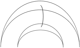
Figure 1: Witten diagram for the four-point function of four heavy BMN states.

The large-spin gauge theory operators in the correlator at hand are dual to the point-like in AdS strings with one angular momentum in $S^{5}$ [8]. The positions of the heavy operators on the boundary are chosen in the form ${\rm x}_{1}=-{\rm x}_{4}$ and ${\rm x}_{2}=-{\rm x}_{3}$. The corresponding Euclidean stationary point solutions for the two semiclassical propagators in fig. 1 are [40]

$$z =\frac{{\rm x}_{14}}{2\mathrm{cosh}(\kappa\tau_{e})}\,,\quad x_{0e}=\frac{{\rm x}_{14}}{2}\tanh(\kappa\tau_{e})\,,\quad x_{i}=0\,,\quad\varphi_{1}=-i\kappa\tau_{e}\,,\quad\kappa=\frac{J}{\sqrt{\lambda}}\,,$$ (3.1a)

$$z^{\prime} =\frac{{\rm x}_{23}}{2\mathrm{cosh}(\kappa^{\prime}\tau^{\prime}_{e})}\,,\quad x^{\prime}_{0e}=\frac{{\rm x}_{23}}{2}\tanh(\kappa^{\prime}\tau^{\prime}_{e})\,,\quad x^{\prime}_{i}=0\,,\quad\varphi^{\prime}_{1}=-i\kappa^{\prime}\tau^{\prime}_{e}\,,\quad\kappa^{\prime}=\frac{J^{\prime}}{\sqrt{\lambda}}\,,$$ (3.1b)

and we assume without loss of generality that ${\rm x}_{14}\geq{\rm x}_{23}$. We denote the respective heavy vertex operators as ${\mathrm{V}}_{J}$ and ${\mathrm{V}}_{J^{\prime}}$, with ${\mathrm{V}}_{-J}\equiv{\mathrm{V}}^{*}_{J}$ and ${\mathrm{V}}_{-J^{\prime}}\equiv{\mathrm{V}}^{*}_{J^{\prime}}$. The two-point function of such operators can be calculated as [7, 8]

$$\langle{\mathrm{V}}_{-J}({\rm x}_{1}){\mathrm{V}}_{J}({\rm x}_{4})\rangle=\frac{1}{{\rm x}_{14}^{2\Delta(J)}}\,,\quad\langle{\mathrm{V}}_{-J^{\prime}}({\rm x}_{2}){\mathrm{V}}_{J^{\prime}}({\rm x}_{3})\rangle=\frac{1}{{\rm x}_{23}^{2\Delta(J^{\prime})}}\,,\quad\Delta(J)=J\,,\quad\Delta(J^{\prime})=J^{\prime}.$$ (3.2)

In order to obtain a contribution to the four-point correlator we need to “join” two two-point functions with a light state, which we choose to be the chiral primary operator. The massless string state corresponding to the CPO originates from the trace of the graviton in the $S^{5}$ directions [42, 43]. Building on results in [10, 44], we conjecture that the bosonic part of the respective supergravity “vertex operator” has the following form

$${\bf V}_{L}(z,x;z^{\prime},x^{\prime})={\bf V}^{(\rm CPO)}_{\Delta}(z,x;z^{\prime},x^{\prime})=\hat{c}_{\Delta}^{2}G_{\Delta}(z,x;z^{\prime},x^{\prime})\,{\rm X}^{j}{\rm X^{\prime}}^{-j}{\cal L}\,{\cal L}^{\prime}\,,\qquad\Delta=j\,,$$ (3.3)

$$G_{\Delta}(z,z;z^{\prime},x^{\prime})=\frac{2^{-\Delta}(\Delta-1)\zeta^{\Delta}}{2\pi^{2}}\ {}_{2}F_{1}\!\left(\frac{\Delta}{2},\frac{\Delta+1}{2};\Delta-1;\zeta^{2}\right),\quad\zeta=\frac{2zz^{\prime}}{z^{2}+z^{\prime 2}+(x-x^{\prime})^{2}}\,,$$

$${\rm X}\equiv X_{1}+iX_{2}=\sin\gamma\cos\psi\,e^{i\varphi_{1}},\qquad{\rm X^{\prime}}\equiv X^{\prime}_{1}+iX^{\prime}_{2}=\sin\gamma^{\prime}\cos\psi^{\prime}\,e^{i\varphi^{\prime}_{1}},$$

$${\cal L}=\frac{\partial x_{m}\bar{\partial}x^{m}-\partial z\bar{\partial}z}{z^{2}}-\partial X_{k}\bar{\partial}X_{k}\,,\qquad{\cal L}^{\prime}=\frac{\partial^{\prime}x^{\prime}_{m}\bar{\partial}^{\prime}x^{\prime m}-\partial^{\prime}z^{\prime}\bar{\partial}^{\prime}z^{\prime}}{z^{\prime 2}}-\partial^{\prime}X^{\prime}_{k}\bar{\partial}^{\prime}X^{\prime}_{k}\,,$$

where the normalization constant $\hat{c}_{\Delta}$ of the CPO is given by [10, 44]

$$\hat{c}_{\Delta}=\hat{c}_{j}=\frac{\sqrt{\lambda}}{8\pi N}(j+1)\sqrt{j}\,.$$ (3.4)

The light gauge theory operator is ${\rm Tr}Z^{j}$ with conformal dimension $\Delta=j\geq 2$. The four-point correlator assumes the form

$$\frac{G_{4}({\rm x}_{1},{\rm x}_{2},{\rm x}_{3},{\rm x}_{4})}{G_{2}({\rm x}_{1},{\rm x}_{4})G^{\prime}_{2}({\rm x}_{2},{\rm x}_{3})}=\int d^{2}\xi d^{2}\xi^{\prime}\,{\bf V}^{(\rm CPO)}_{\Delta}(z,x;z^{\prime},x^{\prime})\,.$$ (3.5)

Evaluated on (3.1), it can be presented as

$$\frac{G_{4}}{G_{2}G^{\prime}_{2}}=16\pi^{2}\hat{c}_{j}^{2}\kappa^{2}\kappa^{\prime 2}\int_{-\infty}^{\infty}d\tau_{e}\int_{-\infty}^{\infty}d\tau^{\prime}_{e}\,\frac{G_{\Delta}e^{j(\kappa\tau_{e}-\kappa^{\prime}\tau^{\prime}_{e})}}{\mathrm{cosh}^{2}(\kappa\tau_{e})\,\mathrm{cosh}^{2}(\kappa^{\prime}\tau^{\prime}_{e})}\,.$$ (3.6)

It can be shown that the bulk-to-bulk propagator for the CPO can be expressed in terms of elementary functions in the following way

$$G_{\Delta}=\frac{\zeta^{j}[(1-\zeta^{2})^{-1/2}+j-2]}{8\pi^{2}(1-\zeta^{2})(1+\sqrt{1-\zeta^{2}})^{j-2}}\,.$$ (3.7)

Let us change the integration variables from $\tau_{e}$ and $\tau^{\prime}_{e}$ to $y\equiv\tanh(\kappa\tau_{e})$ and $y^{\prime}\equiv\tanh(\kappa^{\prime}\tau^{\prime}_{e})$. Then (3.6) becomes

$$\frac{G_{4}}{G_{2}G^{\prime}_{2}}=2\hat{c}_{j}^{2}\kappa\kappa^{\prime}\eta^{j}\int_{-1}^{1}dy\int_{-1}^{1}dy^{\prime}\,\frac{(1+y)^{j}(1-y^{\prime})^{j}}{(1-\eta yy^{\prime})^{j}}\frac{(1-\zeta^{2})^{-1/2}+j-2}{(1-\zeta^{2})(1+\sqrt{1-\zeta^{2}})^{j-2}}\,,$$ (3.8)

where we have introduced

$$\eta=\frac{2{\rm x}_{14}{\rm x}_{23}}{{\rm x}^{2}_{14}+{\rm x}^{2}_{23}}\,.$$

We finally obtain for the contribution to the four-point correlator

$$\frac{G_{4}}{G_{2}G^{\prime}_{2}}=2\hat{c}_{j}^{2}\kappa\kappa^{\prime}\eta^{j}\int_{-1}^{1}dy\int_{-1}^{1}dy^{\prime}\,[I_{1}+(j-2)I_{2}]\,,$$ (3.9)

$$I_{1}=\frac{(1+y)^{j}(1-y^{\prime})^{j}(1-\eta yy^{\prime})}{P^{3/2}(1-\eta yy^{\prime}+\sqrt{P})^{j-2}}\,,\qquad I_{2}=\frac{(1+y)^{j}(1-y^{\prime})^{j}}{P(1-\eta yy^{\prime}+\sqrt{P})^{j-2}}\,,$$

where $P=\eta^{2}(y^{2}+y^{\prime 2})-2\eta yy^{\prime}+1-\eta^{2}$. If we choose for simplicity $j=2$, we will get

$$G_{4}({\rm x}_{1},{\rm x}_{2},{\rm x}_{3},{\rm x}_{4})=\frac{C_{J,J^{\prime}\!,\,j=2}}{{\rm x}_{14}^{2\Delta(J)}\,{\rm x}_{23}^{2\Delta(J^{\prime})}}\,,$$ (3.10)

where

$$C_{J,J^{\prime}\!,2} =2\hat{c}_{2}^{2}\kappa\kappa^{\prime}\eta^{2}\int_{-1}^{1}dy\int_{-1}^{1}dy^{\prime}\,\frac{(1+y)^{2}(1-y^{\prime})^{2}(1-\eta yy^{\prime})}{P^{3/2}}$$

$$=\frac{9JJ^{\prime}}{15\pi^{2}N^{2}}\!\left(\frac{(2\chi-1)(3\chi-1)}{2\chi}-\frac{(3\chi-2)\ln\chi}{\chi-1}\right)\!,\qquad\chi=\frac{({\rm x}_{14}-{\rm x}_{23})^{2}}{({\rm x}_{14}+{\rm x}_{23})^{2}}\,.$$ (3.11)

It can be easily seen that the right-hand expression in (3.10) behaves appropriately under conformal transformations. At first glance the ratio $\chi$ does not look conformally invariant, but if we account for the constraints ${\rm x}_{1}=-{\rm x}_{4}$ and ${\rm x}_{2}=-{\rm x}_{3}$ imposed on the positions of operators, we will see that $\chi$ and $\eta$ are not only invariant under translations, rotations and dilations, but also under inversion, which guarantees their conformal invariance. The existence of only one ratio (instead of two) follows from the constrained nature of operator positions.

4 Conclusion

The duality between gauge and string theories passed through many crucial developments over the last years. The AdS/CFT correspondence has achieved impressive results about the anomalous dimensions of gauge theory operators, integrable structures, etc., and various properties of gauge theories at strong coupling have been established. One of the main challenges ahead is to find efficient methods for calculation of correlation functions.

Although the three-point correlator of three heavy operators is not yet fully understood [33]–[39], we have discovered a lot about the behavior of correlation functions containing two heavy and one light states at strong coupling [10, 11]. Using the trajectory for the correlator of two heavy operators [6, 8], the authors of [12] put forward an approach based on insertion of vertex operators. The same method applies also to higher $n$-point correlation functions with two heavy and $n-2$ light operators.

In the present paper we consider string theory on $AdS_{5}\times S^{5}$ and compute specific leading contributions to four-point functions at strong coupling, applying the ideas of [12] for calculation of correlators with vertex operators. We examine the method in the case of four heavy BMN states.

There has been also development in the computation of three- and four-point correlation functions with heavy operators via integrability techniques [45]–[51]. It would be very interesting to see if our results can be obtained in such a way from the gauge theory point of view.

References

• [1] J. M. Maldacena, “The large $N$ limit of superconformal field theories and supergravity,” Adv. Theor. Math. Phys. 2, 231 (1998) [hep-th/9711200].
• [2] S. S. Gubser, I. R. Klebanov and A. M. Polyakov, “Gauge theory correlators from non-critical string theory,” Phys. Lett. B 428, 105 (1998) [hep-th/9802109].
• [3] E. Witten, “Anti-de Sitter space and holography,” Adv. Theor. Math. Phys. 2, 253 (1998) [hep-th/9802150].
• [4] A. M. Polyakov, “Gauge fields and space-time,” Int. J. Mod. Phys. A 17, 119 (2002) [hep-th/0110196].
• [5] S. S. Gubser, I. R. Klebanov and A. M. Polyakov, “A semi-classical limit of the gauge/string correspondence,” Nucl. Phys. B 636, 99 (2002) [hep-th/0204051].
• [6] A. A. Tseytlin, “On semiclassical approximation and spinning string vertex operators in $AdS_{5}\times S^{5}$,” Nucl. Phys. B 664, 247 (2003) [hep-th/0304139].
• [7] E. I. Buchbinder, “Energy-Spin Trajectories in $AdS_{5}\times S^{5}$ from Semiclassical Vertex Operators,” JHEP 1004, 107 (2010) [arXiv:1002.1716].
• [8] E. I. Buchbinder and A. A. Tseytlin, “On semiclassical approximation for correlators of closed string vertex operators in AdS/CFT,” JHEP 1008, 057 (2010) [arXiv:1005.4516].
• [9] R. A. Janik, P. Surowka and A. Wereszczynski, “On correlation functions of operators dual to classical spinning string states,” JHEP 1005, 030 (2010) [arXiv:1002.4613].
• [10] K. Zarembo, “Holographic three-point functions of semiclassical states,” JHEP 1009, 030 (2010) [arXiv:1008.1059].
• [11] M. S. Costa, R. Monteiro, J. E. Santos and D. Zoakos, “On three-point correlation functions in the gauge/gravity duality,” JHEP 1011, 141 (2010) [arXiv:1008.1070].
• [12] R. Roiban and A. A. Tseytlin, “On semiclassical computation of 3-point functions of closed string vertex operators in $AdS_{5}\times S^{5}$,” Phys. Rev. D 82, 106011 (2010) [arXiv:1008.4921].
• [13] R. Hernández, “Three-point correlation functions from semiclassical circular strings,” J. Phys. A 44, 085403 (2011) [arXiv:1011.0408].
• [14] S. Ryang, “Correlators of Vertex Operators for Circular Strings with Winding Numbers in $AdS_{5}\times S^{5}$,” JHEP 1101, 092 (2011) [arXiv:1011.3573].
• [15] G. Georgiou, “Two and three-point correlators of operators dual to folded string solutions at strong coupling,” JHEP 1102, 046 (2011) [arXiv:1011.5181].
• [16] J. G. Russo and A. A. Tseytlin, “Large spin expansion of semiclassical 3-point correlators in $AdS_{5}\times S^{5}$,” JHEP 1102, 029 (2011) [arXiv:1012.2760].
• [17] C. Park and B. Lee, “Correlation functions of magnon and spike,” Phys. Rev. D 83, 126004 (2011) [arXiv:1012.3293].
• [18] D. Bak, B. Chen and J. Wu, “Holographic Correlation Functions for Open Strings and Branes,” JHEP 1106, 014 (2011) [arXiv:1103.2024].
• [19] A. Bissi, C. Kristjansen, D. Young and K. Zoubos, “Holographic three-point functions of giant gravitons,” JHEP 1106, 085 (2011) [arXiv:1103.4079].
• [20] R. Hernández, “Three-point correlators for giant magnons,” JHEP 1105, 123 (2011) [arXiv:1104.1160].
• [21] X. Bai, B. Lee and C. Park, “Correlation function of dyonic strings,” Phys. Rev. D 84, 026009 (2011) [arXiv:1104.1896].
• [22] L. F. Alday and A. A. Tseytlin, “On strong-coupling correlation functions of circular Wilson loops and local operators,” J. Phys. A 44, 395401 (2011) [arXiv:1105.1537].
• [23] C. Ahn and P. Bozhilov, “Three-point Correlation functions of Giant magnons with finite size,” Phys. Lett. B 702, 286 (2011) [arXiv:1105.3084].
• [24] B. Lee and C. Park, “Finite size effect on the magnon’s correlation functions,” Phys. Rev D 84, 086005 (2011) [arXiv:1105.3279].
• [25] D. Arnaudov and R. C. Rashkov, “Quadratic corrections to three-point functions,” Fortschr. Phys. 60, 217 (2012) [arXiv:1106.0859].
• [26] G. Georgiou, “SL(2) sector: weak/strong coupling agreement of three-point correlators,” JHEP 1109, 132 (2011) [arXiv:1107.1850].
• [27] P. Bozhilov, “More three-point correlators of giant magnons with finite size,” JHEP 1108, 121 (2011) [arXiv:1107.2645].
• [28] L. F. Alday, E. I. Buchbinder and A. A. Tseytlin, “Correlation function of null polygonal Wilson loops with local operators,” JHEP 1109, 034 (2011) [arXiv:1107.5702].
• [29] P. Bozhilov, “Three-point correlators: finite-size giant magnons and singlet scalar operators on higher string levels,” Nucl. Phys. B 855, 268 (2012) [arXiv:1108.3812].
• [30] A. Bissi, T. Harmark and M. Orselli, “Holographic 3-point function at one loop,” JHEP 1202, 133 (2012) [arXiv:1112.5075].
• [31] R. Hernández, “Semiclassical correlation functions of Wilson loops and local vertex operators,” Nucl. Phys. B 862, 751 (2012) [arXiv:1202.4383].
• [32] P. Caputa, R. Koch and K. Zoubos, “Extremal vs. Non-Extremal Correlators with Giant Gravitons,” JHEP 1208, 143 (2012) [arXiv:1204.4172].
• [33] T. Klose and T. McLoughlin, “A light-cone approach to three-point functions in $AdS_{5}\times S^{5}$,” JHEP 1204, 080 (2012) [arXiv:1106.0495].
• [34] S. Ryang, “Extremal Correlator of Three Vertex Operators for Circular Winding Strings in $AdS_{5}\times S^{5}$,” JHEP 1111, 026 (2011) [arXiv:1109.3242].
• [35] R. A. Janik and A. Wereszczynski, “Correlation functions of three heavy operators: The AdS contribution,” JHEP 1112, 095 (2011) [arXiv:1109.6262].
• [36] Y. Kazama and S. Komatsu, “On holographic three point functions for GKP strings from integrability,” JHEP 1201, 110 (2012) [arXiv:1110.3949].
• [37] E. I. Buchbinder and A. A. Tseytlin, “Semiclassical correlators of three states with large $S^{5}$ charges in string theory in $AdS_{5}\times S^{5}$,” Phys. Rev. D 85, 026001 (2012) [arXiv:1110.5621].
• [38] S. Ryang, “Three-Point Correlator of Heavy Vertex Operators for Circular Winding Strings in $AdS_{5}\times S^{5}$,” Phys. Lett. B 713, 122 (2012) [arXiv:1204.3688].
• [39] Y. Kazama and S. Komatsu, “Wave functions and correlation functions for GKP strings from integrability,” JHEP 1209, 022 (2012) [arXiv:1205.6060].
• [40] E. I. Buchbinder and A. A. Tseytlin, “Semiclassical four-point functions in $AdS_{5}\times S^{5}$,” JHEP 1102, 072 (2011) [arXiv:1012.3740].
• [41] D. Arnaudov, R. C. Rashkov and T. Vetsov, “Three- and four-point correlators of operators dual to folded string solutions in $AdS_{5}\times S^{5}$,” Int. J. Mod. Phys. A 26, 3403 (2011) [arXiv:1103.6145].
• [42] H. J. Kim, L. J. Romans and P. van Nieuwenhuizen, “The Mass Spectrum Of Chiral N=2 D=10 Supergravity On S5,” Phys. Rev. D 32, 389 (1985).
• [43] S. Lee, S. Minwalla, M. Rangamani and N. Seiberg, “Three-Point Functions of Chiral Operators in $D=4$, ${\cal N}=4$ SYM at Large $N$,” Adv. Theor. Math. Phys. 2, 697 (1998) [hep-th/9806074]. $\bullet$ G. Arutyunov and S. Frolov, “Some Cubic Couplings in Type IIB Supergravity on $AdS_{5}\times S^{5}$ and Three-point Functions in SYM4 at Large $N$,” Phys. Rev. D 61, 064009 (2000) [hep-th/9907085]. $\bullet$ S. Lee, “AdS5/CFT4 Four-point Functions of Chiral Primary Operators: Cubic Vertices,” Nucl. Phys. B 563, 349 (1999) [hep-th/9907108].
• [44] D. E. Berenstein, R. Corrado, W. Fischler and J. M. Maldacena, “The operator product expansion for Wilson loops and surfaces in the large $N$ limit,” Phys. Rev. D 59, 105023 (1999) [hep-th/9809188].
• [45] J. Escobedo, N. Gromov, A. Sever and P. Vieira, “Tailoring Three-Point Functions and Integrability,” JHEP 1109, 028 (2011) [arXiv:1012.2475].
• [46] J. Escobedo, N. Gromov, A. Sever and P. Vieira, “Tailoring Three-Point Functions and Integrability II. Weak/strong coupling match,” JHEP 1109, 029 (2011) [arXiv:1104.5501].
• [47] J. Caetano and J. Escobedo, “On four-point functions and integrability in ${\cal N}=4$ SYM: from weak to strong coupling,” JHEP 1109, 080 (2011) [arXiv:1107.5580].
• [48] G. Georgiou, V. Gili, A. Grossardt and J. Plefka, “Three-point functions in planar ${\cal N}=4$ super Yang-Mills Theory for scalar operators up to length five at the one-loop order,” JHEP 1204, 038 (2012) [arXiv:1201.0992].
• [49] N. Gromov and P. Vieira, “Quantum Integrability for Three-Point Functions” [arXiv:1202.4103].
• [50] G. Grignani and A. Zayakin, “Matching Three-point Functions of BMN Operators at Weak and Strong coupling,” JHEP 1206, 142 (2012) [arXiv:1204.3096].
• [51] G. Grignani and A. Zayakin, “One-loop three-point functions of BMN operators at weak and strong coupling,” JHEP 1209, 087 (2012) [arXiv:1205.5279].