Upper bounds for packings of spheres of several radii

Abstract.

We give theorems that can be used to upper bound the densities of packings of different spherical caps in the unit sphere and of translates of different convex bodies in Euclidean space. These theorems extend the linear programming bounds for packings of spherical caps and of convex bodies through the use of semidefinite programming. We perform explicit computations, obtaining new bounds for packings of spherical caps of two different sizes and for binary sphere packings. We also slightly improve bounds for the classical problem of packing identical spheres.

1. Introduction

How densely can one pack given objects into a given container? Problems of this sort, generally called packing problems, are fundamental problems in geometric optimization.

An important example having a rich history is the sphere packing problem. Here one tries to place equal-sized spheres with pairwise disjoint interiors into$n$-dimensional Euclidean space while maximizing the fraction of covered space. In two dimensions the best packing is given by placing open disks centered at the points of the hexagonal lattice. In three dimensions, the statement that the best sphere packing has density $\pi/\sqrt{18}=0.7404\ldots$ was known as Kepler’s conjecture; it was proved by Hales [20] in 1998 by means of a computer-assisted proof.

Currently, one of the best methods for obtaining upper bounds for the density of sphere packings is due to Cohn and Elkies [8]. In 2003 they used linear programming to obtain the best known upper bounds for the densities of sphere packings in dimensions $4,\ldots,36$. They almost closed the gap between lower and upper bounds in dimensions $8$ and $24$. Their method is the noncompact version of the linear programming method of Delsarte, Goethals, and Seidel [11] for upper-bounding the densities of packings of spherical caps on the unit sphere.

From a physical point of view, packings of spheres of different sizes are relevant as they can be used to model chemical mixtures which consist of multiple atoms or, more generally, to model the structure of composite material. For more about technological applications of these kind of systems of polydisperse, totally impenetrable spheres we refer to Torquato [39, Chapter 6]. In recent work, Hopkins, Jiao, Stillinger, and Torquato [25, 26] presented lower bounds for the densities of packings of spheres of two different sizes, also called binary sphere packings.

In coding theory, packings of spheres of different sizes are important in the design of error-correcting codes which can be used for unequal error protection. Masnick and Wolf [31] were the first who considered codes with this property.

In this paper we extend the linear programming method of Cohn and Elkies to obtain new upper bounds for the densities of multiple-size sphere packings. We also extend the linear programming method of Delsarte, Goethals, and Seidel to obtain new upper bounds for the densities of multiple-size spherical cap packings.

We perform explicit calculations for binary packings in both cases using semidefinite, instead of linear, programming. In particular we complement the constructive lower bounds of Hopkins, Jiao, Stillinger, and Torquato by non-constructive upper bounds. Insights gained from our computational approach are then used to improve known upper bounds for the densities of monodisperse sphere packings in dimensions $4$, … $9$, except $8$. The bounds we present improve on the best-known bounds due to Cohn and Elkies [8].

1.1. Methods and theorems

We model the packing problems using tools from combinatorial optimization. All possible positions of the objects which we can use for the packing are vertices of a graph and we draw edges between two vertices whenever the two corresponding objects cannot be simultaneously present in the packing because they overlap in their interiors. Now every independent set in this conflict graph gives a valid packing and vice versa. To determine the density of the packing we use vertex weights since we want to distinguish between “small” and “big” objects. For finite graphs it is known that the weighted independence number can be upper bounded by the weighted theta number. Our theorems for packings of spherical caps and spheres are infinite-dimensional analogues of this result.

Let $G=(V,E)$ be a finite graph. A set $I\subseteq V$ is independent if no two vertices in $I$ are adjacent. Given a weight function $w\colon V\to\mathbb{R}_{\geq 0}$, the weighted independence number of $G$ is the maximum weight of an independent set, i.e.,

$$\alpha_{w}(G)=\max\biggl{\{}\sum_{x\in I}w(x):\text{$I\subseteq V$ is independent}\biggr{\}}.$$

Finding $\alpha_{w}(G)$ is an NP-hard problem.

Grötschel, Lovász, and Schrijver [19] defined a graph parameter that gives an upper bound for $\alpha_{w}$ and which can be computed efficiently by semidefinite optimization. It can be presented in many different, yet equivalent ways, but the one convenient for us is

$$\begin{array}[]{rll}\vartheta^{\prime}_{w}(G)=\min&M\\ &K-(w^{1/2})(w^{1/2})^{\sf T}&\text{is positive semidefinite},\\ &K(x,x)\leq M&\text{for all $x\in V$},\\ &K(x,y)\leq 0&\text{for all $\{x,y\}\not\in E$ where $x\neq y$},\\ &\text{$M\in\mathbb{R}$, $K\in\mathbb{R}^{V\times V}$ is symmetric.}\hfil\lx@intercol\lx@intercol\end{array}$$

Here we give a proof of the fact that $\vartheta^{\prime}_{w}(G)$ upper bounds $\alpha_{w}(G)$. In a sense, after discarding the analytical arguments in the proofs of Theorems 1.2 and 1.3, we are left with this simple proof.

Theorem 1.1.

For any finite graph $G=(V,E)$ with weight function $w\colon V\to\mathbb{R}_{\geq 0}$ we have $\alpha_{w}(G)\leq\vartheta^{\prime}_{w}(G)$.

Proof.

Let $I\subseteq V$ be an independent set of nonzero weight and let $K\in\mathbb{R}^{V\times V}$, $M\in\mathbb{R}$ be a feasible solution of $\vartheta^{\prime}_{w}(G)$. Consider the sum

$$\sum_{x,y\in I}w(x)^{1/2}w(y)^{1/2}K(x,y).$$

This sum is at least

$$\sum_{x,y\in I}w(x)^{1/2}w(y)^{1/2}w(x)^{1/2}w(y)^{1/2}=\biggl{(}\sum_{x\in I}w(x)\biggr{)}^{2}$$

because $K-(w^{1/2})(w^{1/2})^{\sf T}$ is positive semidefinite.

The sum is also at most

$$\sum_{x\in I}w(x)K(x,x)\leq M\sum_{x\in I}w(x)$$

because $K(x,x)\leq M$ and because $K(x,y)\leq 0$ whenever $x\neq y$ as $I$ forms an independent set. Now combining both inequalities proves the theorem. ∎

Multiple-size spherical cap packings

We first consider packings of spherical caps of several radii on the unit sphere $S^{n-1}=\{\,x\in\mathbb{R}^{n}:x\cdot x=1\,\}$. The spherical cap with angle $\alpha\in[0,\pi]$ and center $x\in S^{n-1}$ is given by

$$C(x,\alpha)=\{\,y\in S^{n-1}:x\cdot y\geq\cos\alpha\,\}.$$

Its normalized volume equals

$$w(\alpha)=\frac{\omega_{n-1}(S^{n-2})}{\omega_{n}(S^{n-1})}\int_{\cos\alpha}^{1}(1-u^{2})^{(n-3)/2}\,du,$$

where $\omega_{n}(S^{n-1})=(2\pi^{n/2})/\Gamma(n/2)$ is the surface area of the unit sphere. Two spherical caps $C(x_{1},\alpha_{1})$ and $C(x_{2},\alpha_{2})$ intersect in their topological interiors if and only if the inner product of $x_{1}$ and $x_{2}$ lies in the interval $(\cos(\alpha_{1}+\alpha_{2}),1]$. Conversely we have

$$C(x_{1},\alpha_{1})^{\circ}\cap C(x_{2},\alpha_{2})^{\circ}=\emptyset\quad\iff\quad x_{1}\cdot x_{2}\leq\cos(\alpha_{1}+\alpha_{2}).$$

A packing of spherical caps with angles $\alpha_{1}$, …, $\alpha_{N}$ is a union of any number of spherical caps with these angles and pairwise-disjoint interiors. The density of the packing is the sum of the normalized volumes of the constituting spherical caps.

The optimal packing density is given by the weighted independence number of the spherical cap packing graph. This is the graph with vertex set $S^{n-1}\times\{1,\ldots,N\}$, where a vertex $(x,i)$ has weight $w(\alpha_{i})$, and where two distinct vertices $(x,i)$ and $(y,j)$ are adjacent if $\cos(\alpha_{i}+\alpha_{j})<x\cdot y$.

In Section 2 we will extend the weighted theta prime number to the spherical cap packing graph. There we will also derive Theorem 1.2 below, which gives upper bounds for the densities of packings of spherical caps. We will show that the sharpest bound given by this theorem is in fact equal to the theta prime number.

In what follows we denote by $P_{k}^{n}$ the Jacobi polynomial $P^{((n-3)/2,(n-3)/2)}_{k}$ of degree $k$, normalized so that $P_{k}^{n}(1)=1$.

Theorem 1.2.

Let $\alpha_{1}$, …, $\alpha_{N}\in(0,\pi]$ be angles and for $i$, $j=1$, …, $N$ and $k\geq 0$ let $f_{ij,k}$ be real numbers such that $f_{ij,k}=f_{ji,k}$ and $\sum_{k=0}^{\infty}|f_{ij,k}|<\infty$ for all $i$, $j$. Write

(1) $$f_{ij}(u)=\sum_{k=0}^{\infty}f_{ij,k}P^{n}_{k}(u).$$

Suppose the functions $f_{ij}$ satisfy the following conditions:

1. $\bigl{(}f_{ij,0}-w(\alpha_{i})^{1/2}w(\alpha_{j})^{1/2}\bigr{)}_{i,j=1}^{N}$ is positive semidefinite;

2. $\bigl{(}f_{ij,k}\bigr{)}_{i,j=1}^{N}$ is positive semidefinite for $k\geq 1$;

3. $f_{ij}(u)\leq 0$ whenever $-1\leq u\leq\cos(\alpha_{i}+\alpha_{j})$.

Then the density of every packing of spherical caps with angles $\alpha_{1}$, …, $\alpha_{N}$ on the unit sphere $S^{n-1}$ is at most $\max\{\,f_{ii}(1):\text{$i=1$, \ldots,~{}$N$}\,\}$.

When $N=1$, Theorem 1.2 reduces to the linear programming bound for spherical cap packings of Delsarte, Goethals, and Seidel [11]. In Section 4 we use semidefinite programming instead of linear programming to perform explicit computations for $N=2$.

Translational packings of bodies and multiple-size sphere packings

We now deal with packings of spheres with several radii in $\mathbb{R}^{n}$. Theorem 1.3 presented below can be used to find upper bounds for the densities of such packings. In fact, it is more general and can be applied to packings of translates of different convex bodies.

Let $\mathcal{K}_{1}$, …, $\mathcal{K}_{N}$ be convex bodies in $\mathbb{R}^{n}$. A translational packing of $\mathcal{K}_{1}$, …, $\mathcal{K}_{N}$ is a union of translations of these bodies in which any two copies have disjoint interiors. The density of a packing is the fraction of space covered by it. There are different ways to formalize this definition, and questions appear as to whether every packing has a density and so on. We postpone further discussion on this matter until Section 3 where we give a proof of Theorem 1.3.

Our theorem can be seen as an analogue of the weighted theta prime number $\vartheta_{w}^{\prime}$ for the infinite graph $G$ whose vertex set is $\mathbb{R}^{n}\times\{1,\ldots,N\}$ and in which vertices $(x,i)$ and $(y,j)$ are adjacent if $x+\mathcal{K}_{i}$ and $y+\mathcal{K}_{j}$ have disjoint interiors. The weight function we consider assigns weight $\operatorname{vol}\mathcal{K}_{i}$ to vertex $(x,i)\in\mathbb{R}^{n}\times\{1,\ldots,N\}$. We will say more about this interpretation in Section 3.

For the statement of the theorem we need some basic facts from harmonic analysis. Let $f\colon\mathbb{R}^{n}\to\mathbb{C}$ be an $L^{1}$ function. For $u\in\mathbb{R}^{n}$, the Fourier transform of $f$ at $u$ is

$$\hat{f}(u)=\int_{\mathbb{R}^{n}}f(x)e^{-2\pi iu\cdot x}\,dx.$$

We say that function $f$ is a Schwartz function (also called a rapidly-decreasing function) if it is infinitely differentiable, and if any derivative of $f$, multiplied by any power of the variables $x_{1}$, …, $x_{n}$, is a bounded function. The Fourier transform of a Schwartz function is a Schwartz function, too. A Schwartz function can be recovered from its Fourier transform by means of the inversion formula:

$$f(x)=\int_{\mathbb{R}^{n}}\hat{f}(u)e^{2\pi iu\cdot x}\,du$$

for all $x\in\mathbb{R}^{n}$.

Theorem 1.3.

Let $\mathcal{K}_{1}$, …, $\mathcal{K}_{N}$ be convex bodies in $\mathbb{R}^{n}$ and let $f\colon\mathbb{R}^{n}\to\mathbb{R}^{N\times N}$ be a matrix-valued function whose every component $f_{ij}$ is a Schwartz function. Suppose $f$ satisfies the following conditions:

1. the matrix $\bigl{(}\hat{f}_{ij}(0)-(\operatorname{vol}\mathcal{K}_{i})^{1/2}(\operatorname{vol}\mathcal{K}_{j})^{1/2}\bigr{)}_{i,j=1}^{N}$ is positive semidefinite;

2. the matrix of Fourier transforms $\bigl{(}\hat{f}_{ij}(u)\bigr{)}_{i,j=1}^{N}$ is positive semidefinite for every $u\in\mathbb{R}^{n}\setminus\{0\}$;

3. $f_{ij}(x)\leq 0$ whenever $\mathcal{K}_{i}^{\circ}\cap(x+\mathcal{K}_{j}^{\circ})=\emptyset$.

Then the density of any packing of translates of $\mathcal{K}_{1}$, …, $\mathcal{K}_{N}$ in the Euclidean space $\mathbb{R}^{n}$ is at most $\max\{\,f_{ii}(0):\text{$i=1$, \ldots, $N$}\,\}$.

We give a proof of this theorem in Section 3. When $N=1$ and when the convex body $\mathcal{K}_{1}$ is centrally symmetric (an assumption which is in fact not needed) then this theorem reduces to the linear programming method of Cohn and Elkies [8].

We apply this theorem to obtain upper bounds for the densities of binary sphere packings, as we discuss in Section 1.3.

1.2. Computational results for binary spherical cap packings

We applied Theorem 1.2 to compute upper bounds for the densities of binary spherical cap packings. The results we obtained are summarized in the plots of Figure 1.

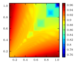
(a) $n=3$

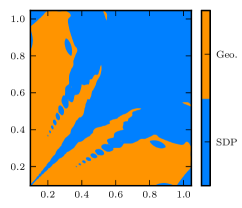
(b) SDP bound/geometric bound for $n=3$

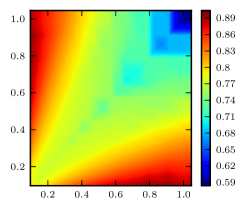
(c) $n=4$

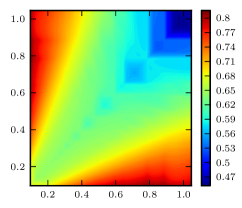
(d) $n=5$

Figure 1. Upper bounds on the packing density for $N=2$. The horizontal and vertical axes carry the spherical cap angle; the colors indicate the density, or in the case of plot (b) whether the SDP bound or the geometric bound is sharper.

For $n=3$, Florian [13, 14] provides a geometric upper bound for the density of a spherical cap packing. He shows that the density of a packing on $S^{2}$ of spherical caps with angles $\alpha_{1},\ldots,\alpha_{N}\in(0,\pi/3]$ is at most

$$\max_{1\leq i\leq j\leq k\leq N}D(\alpha_{i},\alpha_{j},\alpha_{k}),$$

where $D(\alpha_{i},\alpha_{j},\alpha_{k})$ is defined as follows. Let $\mathcal{T}$ be a spherical triangle in $S^{2}$ such that if we center the spherical caps with angles $\alpha_{i}$, $\alpha_{j}$, and $\alpha_{k}$ at the vertices of $\mathcal{T}$, then the caps intersect pairwise at their boundaries. The number $D(\alpha_{i},\alpha_{j},\alpha_{k})$ is then defined as the fraction of the area of $\mathcal{T}$ covered by the caps.

In Figure 1b we see that for $N=2$ it depends on the angles whether the geometric or the semidefinite programming bound is sharper. In particular we see that near the diagonal the semidefinite programming bound is at least as good as the geometric bound; see also Figure 2a.

We can construct natural multiple-size spherical cap packings by taking the incircles of the faces of spherical Archimedean tilings. A sequence of binary packings is for instance obtained by taking the incircles of the prism tilings. These are the Archimedean tilings with vertex figure $(4,4,k)$ for $k\geq 3$ (although strictly speaking for $k=4$ this is a spherical Platonic tiling). The question then is whether the packing associated with the $k$-prism has maximal density among all packings with the same cap angles $\pi/k$ and $\pi/2-\pi/k$, that is, whether the packing is maximal. The packing for $k=3$ is not maximal while the one for $k=4$ trivially is, since here there is only one cap size, and adding a $9$th cap yields a density greater than $1$.

Heppes and Kertész [22] showed that the configurations for $k\geq 6$ are maximal, and the remaining case $k=5$ was later shown to maximal by Florian and Heppes [15]. Florian [13] showed that the geometric bound given above is in fact sharp for the cases where $k\geq 6$, and for the $k=5$ case it is not sharp but still good enough to prove maximality (notice that given a finite number of cap angles, the set of obtainable densities is finite).

Now we illustrate that Theorem 1.2 gives a sharp bound for the density of the packing associated to the $5$-prism, thus giving a simple proof of its maximality. The theorem also provides a sharp bound for $n=4$ but whether it can provide sharp bounds for the cases $n\geq 6$ we do not know at the moment. The numerical results are not decisive.

We shall exhibit functions

$$f_{ij}(u)=\sum_{k=0}^{4}f_{ij,k}P^{n}_{k}(u)$$

which satisfy the conditions of Theorem 1.2 with $f_{11}(1)=5w(\alpha_{1})+2w(\alpha_{2})$ where

$$\alpha_{1}=\frac{\pi}{5},\;\alpha_{2}=\frac{3\pi}{10},\;w(\alpha_{1})=\frac{1}{2}\left(1-\cos\frac{\pi}{5}\right),\;w(\alpha_{2})=\frac{1}{2}\left(1-\cos\frac{3\pi}{10}\right).$$

By complementary slackness of semidefinite optimization the coefficients $f_{ij,k}$ have to satisfy the following linear conditions:

$$0=f_{11}\left(\cos\frac{2\pi}{5}\right)=f_{11}\left(\cos\frac{4\pi}{5}\right)=f^{\prime}_{11}\left(\cos\frac{2\pi}{5}\right)=f_{12}(0)=f_{22}(-1);$$

the product

$$\begin{pmatrix}f_{11,0}&f_{12,0}\\ f_{12,0}&f_{22,0}\end{pmatrix}\begin{pmatrix}25w(\alpha_{1})&10\sqrt{w(\alpha_{1})w(\alpha_{2})}\\ 10\sqrt{w(\alpha_{1})w(\alpha_{2})}&4w(\alpha_{2})\end{pmatrix}$$

equals

$$\begin{pmatrix}25w(\alpha_{1})^{2}+10w(\alpha_{1})w(\alpha_{2})&\sqrt{w(\alpha_{1})w(\alpha_{2})}(10w(\alpha_{1})+4w(\alpha_{2}))\\ \sqrt{w(\alpha_{1})w(\alpha_{2})}(25w(\alpha_{1})+10w(\alpha_{2}))&10w(\alpha_{1})w(\alpha_{2})+4w(\alpha_{2})^{2}\end{pmatrix};$$

for $k=1,\ldots,4$ the product of the two matrices $\begin{pmatrix}f_{11,k}&f_{12,k}\\ f_{12,k}&f_{22,k}\end{pmatrix}$ and

$$\begin{pmatrix}w(\alpha_{1})(5P_{k}(1)+10P_{k}(\cos\frac{2\pi}{5})+10P_{k}(\cos\frac{2\pi}{4}))&\sqrt{w(\alpha_{1})w(\alpha_{2})}10P_{k}(0)\\ \sqrt{w(\alpha_{1})w(\alpha_{2})}10P_{k}(0)&w(\alpha_{2})(2P_{k}(1)+2P_{k}(-1))\end{pmatrix}$$

equals zero. This linear system together with the additional assumptions

$$0=f_{11}(-1)=f_{12}\left(-\frac{95}{100}\right)=f^{\prime}_{12}\left(-\frac{95}{100}\right)$$

has a one-dimensional space of solutions from which it is easy to select one which fulfills all requirements of Theorem 1.2.

For the remaining $13$ Archimedean solids in dimension $n=3$ we are only able to show maximality of the packing associated to the truncated octahedron, the Archimedean solid with vertex figure $(6,6,5)$. Its density is $0.9056\ldots$, the geometric bound shows that the density is at most $0.9088\ldots$, and using the semidefinite program we get $0.9079\ldots$ as an upper bound. The first packing with caps of angles $\arcsin(1/3)$ and $\arcsin(1/\sqrt{3})$ which would be denser is obtained by taking $19$ of the smaller caps and $4$ of the bigger caps, and has density $0.9103\ldots$ The upper bounds show however that it is not possible to obtain this dense a packing, thus showing that the truncated octahedron packing is maximal.

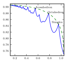
(a) $n=3$

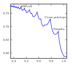
(b) $n=4$

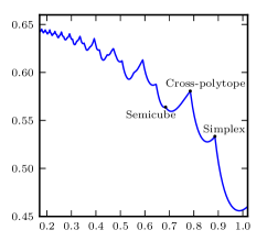
(c) $n=5$

Figure 2. Upper bounds on the packing density for $N=1$, the horizontal axis carries the spherical cap angle and the vertical axis the packing density.

We also used our programs to plot the upper bounds for $N=1$, the classical linear programming bound of Delsarte, Goethals, and Seidel [11], for dimensions $n=3$, $4$, and $5$ in Figure 2. To the best of our knowledge these kinds of plots were not made before and they seem to reveal interesting properties of the bound. For better orientation we show in the plots the packings where the linear programming bound is sharp (cf. Levenshtein [28]; Cohn and Kumar [9] proved the much stronger statement that these packings provide point configurations which are universally optimal). The dotted line in the plot for $n=3$ is the geometric bound, and since we know that both the geometric (cf. Florian [13]) and the semidefinite programming bounds are sharp for the given configurations, we know that at these peaks the bounds meet.

An interesting feature of the upper bound seems to be that it has some periodic behavior. Indeed, the numerical results suggest that for $n=3$, the two bounds in fact meet infinitely often as the angle decreases, and that between any two of these meeting points the semidefinite programming bound has a similar shape. Although in higher dimensions we do not have a geometric bound, the semidefinite programming bound seems to admit the same kind of periodic behavior.

1.3. Computational results for binary sphere packings

We applied Theorem 1.3 to compute upper bounds for the densities of binary sphere packings. The results we obtained are summarized in the plot of Figure 3, where we show bounds computed for dimensions $2$, …, $5$. A detailed account of our approach is given in Section 5. We now quickly discuss the bounds presented in Figure 3.

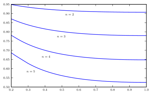
Figure 3. The horizontal axis carries the ratio between the radii of the small and the large spheres. The vertical axis carries our upper bound. Our bounds for dimensions $2$, …, $5$ are shown together.

Dimension 2. Only in dimension $2$ have binary sphere (i.e., circle) packings been studied in depth. We refer to the introduction in the paper of Heppes [21] which surveys the known results about binary circle packings in the plane.

Currently one of the best-known upper bounds for the maximum density of a binary circle packing is due to Florian [12]. Florian’s bound states that a packing of circles in which the ratio between the radii of the smallest and largest circles is $r$ has density at most

$$\frac{\pi r^{2}+2(1-r^{2})\arcsin(r/(1+r))}{2r\sqrt{2r+1}},$$

and that this bound is achieved exactly for $r=1$ (i.e., for classical circle packings) and for $r=0$ in the limit.

The question arises of which bound is better, our bound or Florian’s bound. From our experiments, it seems that our bound is worse than Florian’s bound, at least for $r<1$. For instance, for $r=1/2$ we obtain the upper bound $0.9174426\ldots$, whereas Florian’s bound is $0.9158118\ldots$ Whether this really means that the bound of Theorem 1.3 is worse than Florian’s bound, or just that the computational approach of Section 5 is too restrictive to attain his bound, we do not know.

It is interesting to note that for $r=1$, that is, for packings of circles of one size, our bound clearly coincides with the one of Cohn and Elkies [8]. This bound seems to be equal to $\pi/\sqrt{12}$, but no proof of this is known.

Dimension 3. Much less is known in dimension $3$. In fact we do not know about other attempts to find upper bounds for the densities of binary sphere packings in dimensions $3$ and higher.

Let us compare our upper bound with the lower bound by Hopkins, Jiao, Stillinger, and Torquato [25]. The record holder for $r\geq 0.2$ in terms of highest density occurs for $r=0.224744\ldots$ and its density is $0.824539\ldots$ Our computations show that there cannot be a packing with this $r$ having density more than $0.8617125\ldots$, so this leaves a margin of $5\%$.

Another interesting case is $r=\sqrt{2}-1=0.414\ldots$ Here the best-known lower bound of $0.793\ldots$ comes from the NaCl-alloy. The large spheres are centered at a face centered cubic lattice and the small spheres are centered at a translated copy of the face centered cubic lattice so that they form a jammed packing. Our upper bound for $r=\sqrt{2}-1$ is $0.813\ldots$, less than $3\%$ away from the lower bound. Therefore, we believe that proving optimality of the NaCl-alloy might be doable.

Dimension 4 and beyond. In higher dimensions even less is known about binary sphere packings. We observed from Figure 3 that it seems that the upper bound is decreasing: as the radius of the small sphere increases from $0.2$ to $1$, the bound seems to decrease. This suggests that the bound given by Theorem 1.3 is decreasing in this sense, but we do not know a proof of this.

We also do not know the limit behavior of our bound when $r$ approaches $0$. Due to numerical instabilities we could not perform numerical calculations in this regime of $r$.

1.4. Improving the Cohn-Elkies bounds

We now present a theorem that can be used to find better upper bounds for the densities of monodisperse sphere packings than those provided by Cohn and Elkies [8]; our theorem is a strengthening of theirs.

Fix $\varepsilon>0$. Given a packing of spheres of radius $1/2$, we consider its $\varepsilon$-tangency graph, a graph whose vertices are the spheres in the packing, and in which two vertices are adjacent if the distance between the centers of the respective spheres lies in the interval $[1,1+\varepsilon)$.

Let $M(\varepsilon)$ be the least upper bound on the average degree of the $\varepsilon$-tangency graph of any sphere packing. Our theorem is the following:

Theorem 1.4.

Take $0=\varepsilon_{0}<\varepsilon_{1}<\cdots<\varepsilon_{m}$ and let $f\colon\mathbb{R}^{n}\to\mathbb{R}$ be a Schwartz function such that

1. $\hat{f}(0)\geq\operatorname{vol}B$, where $B$ is the ball of radius $1/2$;

2. $\hat{f}(u)\geq 0$ for all $u\in\mathbb{R}^{n}\setminus\{0\}$;

3. $f(x)\leq 0$ whenever $\|x\|\geq 1+\varepsilon_{m}$;

4. $f(x)\leq\eta_{k}$ whenever $\|x\|\in[1+\varepsilon_{k-1},1+\varepsilon_{k})$ with $\eta_{k}\geq 0$, for $k=1$, …, $m$.

Then the density of a sphere packing is at most the optimal value of the following linear programming problem in variables $A_{1}$, …, $A_{m}$:

(2) $$\begin{array}[]{rll}\max&f(0)+\eta_{1}A_{1}+\cdots+\eta_{m}A_{m}\\ &A_{1}+\cdots+A_{k}\leq U(\varepsilon_{k})&\text{for~{}$k=1$, \ldots,~{}$m$},\\ &A_{i}\geq 0&\text{for~{}$i=1$, \ldots,~{}$m$},\end{array}$$

where $U(\varepsilon_{k})\geq M(\varepsilon_{k})$ for $k=1$, …, $m$.

In Section 6 we give a proof of Theorem 1.4 and show how to compute upper bounds for $M(\varepsilon)$ using the semidefinite programming bounds of Bachoc and Vallentin [4] for the sizes of spherical codes. There we also show how to use semidefinite programming and the same ideas we employ in the computations for binary sphere packings (cf. Section 5) to compute better upper bounds for the densities of sphere packings.

In Table 1 we show the upper bounds obtained through our application of Theorem 1.4. To better compare our bounds with those of Cohn and Elkies, on Table 1 we show bounds for the center density of a packing, the center density of a packing of unit spheres being equal to $\Delta/\operatorname{vol}B$, where $\Delta$ is the density of the packing, and $B$ is a unit ball.

We omit dimension $8$ because for this dimension it is already believed that the Cohn-Elkies bound is itself optimal, and therefore as is to be expected we did not manage to obtain any improvement over their bound. We also note that the bounds by Cohn and Elkies are the best known upper bounds in all other dimensions shown.

Dimension	Lower bound	Cohn-Elkies bound	New upper bound
$4$	0.12500	0.13126	0.130587
$5$	0.08839	0.09975	0.099408
$6$	0.07217	0.08084	0.080618
$7$	0.06250	0.06933	0.069193
$9$	0.04419	0.05900	0.058951

Table 1. For each dimension we show the best lower bound known, the bound by Cohn and Elkies [8], and the upper bound coming from Theorem 1.4.

In dimension $3$ the Cohn-Elkies bound is $0.18616$ whereas the optimal sphere packing has center density $0.17678$. We can improve the Cohn-Elkies bound to $0.184559$ which is also better than the upper bound $0.1847$ due to Rogers [33].

2. Multiple-size spherical cap packings

In this section we prove Theorem 1.2 and discuss its relation to an extension of the weighted theta prime number for the spherical cap packing graph.

2.1. Proof of Theorem 1.2

Let $x_{1}$, …, $x_{m}\in S^{n-1}$ and $r\colon\{1,\ldots,m\}\to\{1,\ldots,N\}$ be such that

$$\bigcup_{i=1}^{m}C(x_{i},\alpha_{r(i)})$$

is a packing of spherical caps on $S^{n-1}$.

Consider the sum

(3) $$\sum_{i,j=1}^{m}w(\alpha_{r(i)})^{1/2}w(\alpha_{r(j)})^{1/2}f_{r(i)r(j)}(x_{i}\cdot x_{j}).$$

By expanding $f_{r(i)r(j)}(x_{i}\cdot x_{j})$ according to (1) this sum is equal to

$$\sum_{k=0}^{\infty}\sum_{i,j=1}^{m}w(\alpha_{r(i)})^{1/2}w(\alpha_{r(j)})^{1/2}f_{r(i)r(j),k}P_{k}^{n}(x_{i}\cdot x_{j}).$$

By the addition formula (cf. e.g. Section 9.6 of Andrews, Askey, and Roy [1]) for the Jacobi polynomials $P_{k}^{n}$ the matrix $\bigl{(}P_{k}^{n}(x_{i}\cdot x_{j})\bigr{)}_{i,j=1}^{m}$ is positive semidefinite. From condition (ii) of the theorem, we also know that the matrix $\bigl{(}f_{r(i)r(j),k}\bigr{)}_{i,j=1}^{m}$ is positive semidefinite for $k\geq 1$. So the inner sum above is nonnegative for $k\geq 1$. If we then consider only the summand for $k=0$ we see that (3) is at least

(4) $$\sum_{i,j=1}^{m}w(\alpha_{r(i)})^{1/2}w(\alpha_{r(j)})^{1/2}f_{r(i)r(j),0}P_{0}^{n}(x_{i}\cdot x_{j})\geq\biggl{(}\sum_{i=1}^{m}w(\alpha_{i})\biggr{)}^{2},$$

where the inequality follows from condition (i) of the theorem.

Now, notice that whenever $i\neq j$, the caps $C(x_{i},\alpha_{r(i)})$ and $C(x_{j},\alpha_{r(j)})$ have disjoint interiors. Condition (iii) then implies that $f_{r(i)r(j)}(x_{i}\cdot x_{j})\leq 0$. So we see that (3) is at most

(5) $$\sum_{i=1}^{m}w(\alpha_{i})f_{r(i)r(i)}(1)\leq\max\{\,f_{ii}(1):\text{$i=1$, \ldots,~{}$N$}\,\}\sum_{i=1}^{m}w(\alpha_{i}).$$

So (3) is at least (4) and at most (5), yielding

$$\sum_{i=1}^{m}w(\alpha_{i})\leq\max\{\,f_{ii}(1):\text{$i=1$, \ldots,~{}$N$}\,\}.\qquad\qed$$

2.2. Theorem 1.2 and the Lovász theta number

We now briefly discuss a generalization of $\vartheta^{\prime}_{w}$ to infinite graphs and its relation to the bound of Theorem 1.2. Similar ideas were developed by Bachoc, Nebe, Oliveira, and Vallentin [3].

Let $G=(V,E)$ be a graph, where $V$ is a compact space, and let $w\colon V\to\mathbb{R}_{\geq 0}$ be a continuous weight function. An element in the space $\mathcal{C}(V\times V)$ of real-valued continuous functions over $V\times V$ is called a kernel. A kernel $K$ is symmetric if $K(x,y)=K(y,x)$ for all $x,y\in V$. It is positive if it is symmetric and if for any $N\in\mathbb{N}$ and for any $x_{1}$, …, $x_{N}\in V$, the matrix $\bigl{(}K(x_{i},x_{j})\bigr{)}_{i,j=1}^{N}$ is positive semidefinite. The weighted theta prime number of $G$ is defined as

(6) $$\begin{array}[]{rll}\vartheta^{\prime}_{w}(G)=\inf&M\\ &K-w^{1/2}\otimes(w^{1/2})^{*}&\text{is a positive kernel},\\ &K(x,x)\leq M&\text{for all $x\in V$},\\ &K(x,y)\leq 0&\text{for all $\{x,y\}\not\in E$ where $x\neq y$},\\ &\text{$M\in\mathbb{R}$, $K\in\mathcal{C}(V\times V)$ is symmetric}.\hfil\lx@intercol\lx@intercol\\ \end{array}$$

One may show, mimicking the proof of Theorem 1.1, that $\vartheta^{\prime}_{w}(G)\geq\alpha_{w}(G)$.

Let $G=(V,E)$ be the spherical cap packing graph as defined in Section 1.1. We will use the symmetry of this graph to show that (6) gives the sharpest bound obtainable by Theorem 1.2.

The orthogonal group $\operatorname{O}(n)$ acts on $S^{n-1}$, and this defines the action of $\operatorname{O}(n)$ on the vertex set $V=S^{n-1}\times\{1,\ldots,N\}$ by $A(x,i)=(Ax,i)$ for $A\in\operatorname{O}(n)$. The group average of a kernel $K\in\mathcal{C}(V\times V)$ is given by

$$\overline{K}((x,i),(y,j))=\int_{\operatorname{O}(n)}K(A(x,i),A(y,j))\,d\mu(A),$$

where $\mu$ is the Haar measure on $\operatorname{O}(n)$ normalized so that $\mu(\operatorname{O}(n))=1$. If $(K,M)$ is feasible for (6), then $(\overline{K},M)$ is feasible too. This follows since for each $A\in\operatorname{O}(n)$, a point $(x,i)$ has the same weight as $A(x,i)$, and two points $(x,i)$ and $(y,j)$ are adjacent if and only if $A(x,i)$ and $A(y,j)$ are adjacent. Since $(K,M)$ and $(\overline{K},M)$ have the same objective value $M$, and since $\overline{K}$ is invariant under the action of $\operatorname{O}(n)$, we may restrict to $\operatorname{O}(n)$-invariant kernels (i.e., kernels $K$ such that $K(Au,Av)=K(u,v)$ for all $A\in\operatorname{O}(n)$ and $u$, $v\in V$) in finding the infimum of (6).

Schoenberg [34] showed that a symmetric kernel $K\in\mathcal{C}(S^{n-1}\times S^{n-1})$ is positive and $\operatorname{O}(n)$-invariant if and only if it lies in the cone spanned by the kernels $(x,y)\mapsto P_{k}^{n}(x\cdot y)$. We will use the following generalization for kernels over $V\times V$.

Theorem 2.1.

A symmetric kernel $K\in\mathcal{C}(V\times V)$, with $V=S^{n-1}\times\{1,\ldots,N\}$, is positive and $\operatorname{O}(n)$-invariant if and only if

(7) $$K((x,i),(y,j))=f_{ij}(x\cdot y)$$

with

$$f_{ij}(u)=\sum_{k=0}^{\infty}f_{ij,k}P_{k}^{n}(u),$$

where $\bigl{(}f_{ij,k}\bigr{)}_{i,j=1}^{N}$ is positive semidefinite for all $k\geq 0$ and $\sum_{k=0}^{\infty}|f_{ij,k}|<\infty$ for all $i$, $j=1$, …, $N$, implying in particular that we have uniform convergence above.

Before we prove the theorem we apply it to simplify problem (6). If $K$ is an $\operatorname{O}(n)$-invariant feasible solution of (6), then $K-w^{1/2}\otimes(w^{1/2})^{*}$ is a positive $\operatorname{O}(n)$-invariant kernel, and hence can be written in the form (7). Using in addition that $P_{0}^{n}=1$, problem (6) reduces to

$$\begin{array}[]{rll}\vartheta^{\prime}_{w}(G)=\inf&M\\ &f_{ii}(0)+w(\alpha_{i})\leq M&\text{for all $1\leq i\leq N$},\\ &f_{ij}(u)+(w(\alpha_{i})w(\alpha_{j}))^{1/2}\leq 0&\text{when $-1\leq u\leq\cos(\alpha_{i}+\alpha_{j})$},\\ &\text{$M\in\mathbb{R}$ and $\bigl{(}f_{ij,k}\bigr{)}_{i,j=1}^{N}$ positive semidefinite for all $k\geq 0$}.\hfil\lx@intercol\lx@intercol\end{array}$$

By substituting $f_{ij,0}-(w(\alpha_{i})w(\alpha_{j}))^{1/2}$ for $f_{ij,0}$ we see that the solution to this problem indeed equals the sharpest bound given by Theorem 1.2.

Proof of Theorem 2.1.

If we endow the space $\mathcal{C}(S^{n-1})$ of real-valued continuous function on the unit sphere $S^{n-1}$ with the usual $L^{2}$ inner product, then for $f$, $g\in\mathcal{C}(V)$,

$$\langle f,g\rangle=\sum_{i=1}^{N}\int_{S^{n-1}}f(x,i)g(x,i)\,d\omega(x)$$

gives an inner product on $\mathcal{C}(V)$. The space $\mathcal{C}(S^{n-1})$ decomposes orthogonally as

$$\mathcal{C}(S^{n-1})=\bigoplus_{k=0}^{\infty}H_{k},$$

where $H_{k}$ is the space of homogeneous harmonic polynomials of degree $k$ restricted to $S^{n-1}$. With

$$H_{k,i}=\{\,f\in\mathcal{C}(V):\text{there is a $g\in H_{k}$ such that $f(\cdot,j)=\delta_{ij}g(\cdot)$}\,\},$$

it follows that $\mathcal{C}(V)$ decomposes orthogonally as

$$\mathcal{C}(V)=\bigoplus_{k=0}^{\infty}\bigoplus_{i=1}^{N}H_{k,i}.$$

Given the action of $\operatorname{O}(n)$ on $V$, we have the natural unitary representation on $\mathcal{C}(V)$ given by $(Af)(x,i)=f(A^{-1}x,i)$ for $A\in\operatorname{O}(n)$ and $f\in\mathcal{C}(V)$. It follows that each space $H_{k,i}$ is $\operatorname{O}(n)$-irreducible and that two spaces $H_{k,i}$ and $H_{k^{\prime},i^{\prime}}$ are $\operatorname{O}(n)$-equivalent if and only if $k=k^{\prime}$. Let

$$\{\,e_{k,i,l}:\text{$k\geq 0$, $1\leq i\leq N$, and $1\leq l\leq h_{k}$}\,\}$$

be a complete orthonormal system of $\mathcal{C}(V)$ such that $e_{k,i,1},$ …, $e_{k,i,h_{k}}$ is a basis of $H_{k,i}$. By Bochner’s characterization [5], a kernel $K\in\mathcal{C}(V\times V)$ is positive and $\operatorname{O}(n)$-invariant if and only if

(8) $$K((x,i),(y,j))=\sum_{k=0}^{\infty}\sum_{i^{\prime},j^{\prime}=1}^{N}f_{ij,k}\sum_{l=1}^{h_{k}}e_{k,i^{\prime},l}(x,i)e_{k,j^{\prime},l}(y,j),$$

where each $\bigl{(}f_{ij,k}\bigr{)}_{i,j=1}^{N}$ is positive semidefinite and $\sum_{k=0}^{\infty}|f_{ij,k}|<\infty$ for all $i$, $j$.

By the addition formula (cf. Chapter 9.6 of Andrews, Askey, and Roy [1]) we have

$$\sum_{l=1}^{h_{k}}e_{k,l}(x)e_{k,l}(y)=\frac{h_{k}}{\omega_{n}(S^{n-1})}P_{k}^{n}(x\cdot y)$$

for any orthonormal basis $e_{k,1},\ldots,e_{k,h_{k}}$ of $H_{k}$. It follows that

$$\sum_{l=1}^{h_{k}}e_{k,i^{\prime},l}(x,i)e_{k,j^{\prime},l}(y,j)=\delta_{ii^{\prime}}\delta_{jj^{\prime}}\frac{h_{k}}{\omega_{n}(S^{n-1})}P_{k}^{n}(x\cdot y),$$

and substituting this into (8) completes the proof. ∎

Bochner’s characterization for the kernel $K$, which we used above, usually assumes that the spaces under consideration are homogeneous, so that the decompositions into isotypic irreducible spaces are guaranteed to be finite. This finiteness is then used to conclude uniform convergence. Since the action of $\operatorname{O}(n)$ on $V$ is not transitive, we do not immediately have this guarantee. We can still use the characterization, however, since irreducible subspaces of $\mathcal{C}(V)$ have finite multiplicity.

3. Translational packings of bodies and multiple-size sphere packings

Before giving a proof of Theorem 1.3 we quickly present some technical considerations regarding density. Here we follow closely Appendix A of Cohn and Elkies [8].

Let $\mathcal{K}_{1}$, …, $\mathcal{K}_{N}$ be convex bodies and $\mathcal{P}$ be a packing of translated copies of $\mathcal{K}_{1}$, …, $\mathcal{K}_{N}$, that is, $\mathcal{P}$ is a union of translated copies of the bodies, any two copies having disjoint interiors. We say that the density of $\mathcal{P}$ is $\Delta$ if for all $p\in\mathbb{R}^{n}$ we have

$$\Delta=\lim_{r\to\infty}\frac{\operatorname{vol}(B(p,r)\cap\mathcal{P})}{\operatorname{vol}B(p,r)},$$

where $B(p,r)$ is the ball of radius $r$ centered at $p$. Not every packing has a density, but every packing has an upper density given by

$$\limsup_{r\to\infty}\sup_{p\in\mathbb{R}^{n}}\frac{\operatorname{vol}(B(p,r)\cap\mathcal{P})}{\operatorname{vol}B(p,r)}.$$

We say that a packing $\mathcal{P}$ is periodic if there is a lattice $L\subseteq\mathbb{R}^{n}$ that leaves $\mathcal{P}$ invariant, that is, which is such that $\mathcal{P}=x+\mathcal{P}$ for all $x\in L$. In other words, a periodic packing consists of some translated copies of the bodies $\mathcal{K}_{1}$, …, $\mathcal{K}_{N}$ arranged inside the fundamental parallelotope of $L$, and this arrangement repeats itself at each copy of the fundamental parallelotope translated by vectors of the lattice.

It is easy to see that a periodic packing has a density. This is particularly interesting for us, since in computing upper bounds for the maximum possible density of a packing we may restrict ourselves to periodic packings, as it is known (and easy to see) that the supremum of the upper densities of packings is also achieved by periodic packings (cf. Appendix A in Cohn and Elkies [8]).

To provide a proof of the theorem we need another fact from harmonic analysis, the Poisson summation formula. Let $f\colon\mathbb{R}^{n}\to\mathbb{C}$ be a Schwartz function and $L\subseteq\mathbb{R}^{n}$ be a lattice. The Poisson summation formula states that, for every $x\in\mathbb{R}^{n}$,

$$\sum_{v\in L}f(x+v)=\frac{1}{\operatorname{vol}(\mathbb{R}^{n}/L)}\sum_{u\in L^{*}}\hat{f}(u)e^{2\pi iu\cdot x},$$

where $L^{*}=\{\,u\in\mathbb{R}^{n}:\text{$u\cdot x\in\mathbb{Z}$ for all~{}$x\in L$}\,\}$ is the dual lattice of $L$ and where $\operatorname{vol}(\mathbb{R}^{n}/L)$ is the volume of a fundamental domain of the lattice $L$.

Proof of Theorem 1.3.

As observed above, we may restrict ourselves to periodic packings. Let then $L\subseteq\mathbb{R}^{n}$ be a lattice and $x_{1}$, …, $x_{m}\in\mathbb{R}^{n}$ and $r\colon\{1,\ldots,m\}\to\{1,\ldots,N\}$ be such that

$$\mathcal{P}=\bigcup_{v\in L}\bigcup_{i=1}^{m}v+x_{i}+\mathcal{K}_{r(i)}$$

is a packing. This means that, whenever $i\neq j$ or $v\neq 0$, bodies $x_{i}+\mathcal{K}_{r(i)}$ and $v+x_{j}+\mathcal{K}_{r(j)}$ have disjoint interiors. This packing is periodic and therefore has a well-defined density, which equals

$$\frac{1}{\operatorname{vol}(\mathbb{R}^{n}/L)}\sum_{i=1}^{m}\operatorname{vol}\mathcal{K}_{r(i)}.$$

Consider the sum

(9) $$\sum_{v\in L}\sum_{i,j=1}^{m}(\operatorname{vol}\mathcal{K}_{r(i)})^{1/2}(\operatorname{vol}\mathcal{K}_{r(j)})^{1/2}f_{r(i)r(j)}(v+x_{j}-x_{i}).$$

Applying the Poisson summation formula we may express (9) in terms of Fourier transform of $f$, obtaining

$$\frac{1}{\operatorname{vol}(\mathbb{R}^{n}/L)}\sum_{u\in L^{*}}\sum_{i,j=1}^{m}(\operatorname{vol}K_{r(i)})^{1/2}(\operatorname{vol}K_{r(j)})^{1/2}\hat{f}_{r(i)r(j)}(u)e^{2\pi iu\cdot(x_{j}-x_{i})},$$

where $L^{*}$ is the dual lattice of $L$.

Since $f$ satisfies condition (ii) of the theorem, matrix $\bigl{(}\hat{f}_{r(i)r(j)}(u)\bigr{)}_{i,j=1}^{m}$ is positive semidefinite for every $u\in\mathbb{R}^{n}$. So the inner sum above is always nonnegative. If we then consider only the summand for $u=0$, we see that (9) is at least

(10) $$\begin{split}&\frac{1}{\operatorname{vol}(\mathbb{R}^{n}/L)}\sum_{i,j=1}^{m}(\operatorname{vol}\mathcal{K}_{r(i)})^{1/2}(\operatorname{vol}\mathcal{K}_{r(j)})^{1/2}\hat{f}_{r(i)r(j)}(0)\\ &\qquad{}\geq\frac{1}{\operatorname{vol}(\mathbb{R}^{n}/L)}\sum_{i,j=1}^{m}\operatorname{vol}\mathcal{K}_{r(i)}\operatorname{vol}\mathcal{K}_{r(j)}\\ &\qquad{}=\frac{1}{\operatorname{vol}(\mathbb{R}^{n}/L)}\biggl{(}\sum_{i=1}^{m}\operatorname{vol}\mathcal{K}_{r(i)}\biggr{)}^{2},\end{split}$$

where the inequality comes from condition (i) of the theorem.

Now, notice that whenever $v\neq 0$ or $i\neq j$ one has $f_{r(i)r(j)}(v+x_{j}-x_{i})\leq 0$. Indeed, since $\mathcal{P}$ is a packing, if $v\neq 0$ or $i\neq j$ then the bodies $x_{i}+\mathcal{K}_{r(i)}$ and $v+x_{j}+\mathcal{K}_{r(j)}$ have disjoint interiors. But then also $\mathcal{K}_{r(i)}$ and $v+x_{j}-x_{i}+\mathcal{K}_{r(j)}$ have disjoint interiors, and then from (iii) we see that $f_{r(i)r(j)}(v+x_{j}-x_{i})\leq 0$.

From this observation we see immediately that (9) is at most

(11) $$\sum_{i=1}^{m}\operatorname{vol}\mathcal{K}_{r(i)}f_{r(i)r(i)}(0)\leq\max\{\,f_{ii}(0):\text{$i=1$, \ldots,~{}$N$}\,\}\sum_{i=1}^{m}\operatorname{vol}\mathcal{K}_{r(i)}.$$

So (9) is at least (10) and at most (11). Putting it all together we get that

$$\frac{1}{\operatorname{vol}(\mathbb{R}^{n}/L)}\sum_{i=1}^{m}\operatorname{vol}\mathcal{K}_{r(i)}\leq\max\{\,f_{ii}(0):\text{$i=1$, \ldots,~{}$N$}\,\},$$

proving the theorem. ∎

We mentioned in the beginning of the section that Theorem 1.3 is an analogue of the weighted theta prime number for a certain infinite graph. The connection will become more clear after we present a slightly more general version of Theorem 1.3.

An $L^{\infty}$ function $f\colon\mathbb{R}^{n}\to\mathbb{C}^{N\times N}$ is said to be of positive type if $f(x)=f(-x)^{*}$ for all $x\in\mathbb{R}^{n}$ and for all $L^{1}$ functions $\rho\colon\mathbb{R}^{n}\to\mathbb{C}^{N}$ we have

$$\int_{\mathbb{R}^{n}}\int_{\mathbb{R}^{n}}\rho(y)^{*}f(x-y)\rho(x)\,dxdy\geq 0.$$

When $N=1$ we have the classical theory of functions of positive type (see e.g. the book by Folland [16] for background). Many useful properties of such functions can be extended to the matrix-valued case (that is, to the $N>1$ case) via a simple observation: a function $f\colon\mathbb{R}^{n}\to\mathbb{C}^{N\times N}$ is of positive type if and only if for all $p\in\mathbb{C}^{N}$ the function $g_{p}\colon\mathbb{R}^{n}\to\mathbb{C}$ such that

$$g_{p}(x)=p^{*}f(x)p$$

is of positive type.

From this observation two useful classical characterizations of functions of positive type can be extended to the matrix-valued case. The first one is useful when dealing with continuous functions of positive type. It states that a continuous and bounded function $f\colon\mathbb{R}^{n}\to\mathbb{C}^{N\times N}$ is of positive type if and only if for every choice $x_{1}$, …, $x_{m}$ of finitely many points in $\mathbb{R}^{n}$, the block matrix $\bigl{(}f(x_{i}-x_{j})\bigr{)}_{i,j=1}^{m}$ is positive semidefinite.

The second characterization is given in terms of the Fourier transform. It states that an $L^{1}$ function $f\colon\mathbb{R}^{n}\to\mathbb{C}^{N\times N}$ is of positive type if and only if the matrix $\bigl{(}\hat{f}_{ij}(u)\bigr{)}_{i,j=1}^{N}$ is positive semidefinite for all $u\in\mathbb{R}^{n}$. So in the statement of Theorem 1.3, for instance, one could replace condition (i) by the equivalent condition that $f$ be a function of positive type.

When $N=1$, the previous two characterizations of functions of positive type date back to Bochner [6].

With this we may give an alternative and more general version of Theorem 1.3.

Theorem 3.1.

Let $\mathcal{K}_{1}$, …, $\mathcal{K}_{N}$ be convex bodies in $\mathbb{R}^{n}$ and let $f\colon\mathbb{R}^{n}\to\mathbb{R}^{N\times N}$ be a continuous and $L^{1}$ function. Suppose $f$ satisfies the following conditions:

1. the matrix $\bigl{(}\hat{f}_{ij}(0)-(\operatorname{vol}\mathcal{K}_{i})^{1/2}(\operatorname{vol}\mathcal{K}_{j})^{1/2}\bigr{)}_{i,j=1}^{N}$ is positive semidefinite;

2. $f$ is of positive type;

3. $f_{ij}(x)\leq 0$ whenever $\mathcal{K}_{i}^{\circ}\cap(x+\mathcal{K}_{j}^{\circ})=\emptyset$.

Then the density of every packing of translates of $\mathcal{K}_{1}$, …, $\mathcal{K}_{N}$ in the Euclidean space $\mathbb{R}^{n}$ is at most $\max\{\,f_{ii}(0):\text{$i=1$, \ldots,~{}$N$}\,\}$.

Let $V=\mathbb{R}^{n}\times\{1,\ldots,N\}$. Notice that the kernel $K\colon V\times V\to\mathbb{R}$ such that

$$K((x,i),(y,j))=f_{ij}(x-y),$$

implicitly defined by the function $f$, plays the same role as the matrix $K$ from the definition of the theta prime number (cf. Section 2.2). For instance, this is a positive kernel, since $f$ is of positive type and hence for any $L^{1}$ function $\rho\colon V\to\mathbb{R}$ we have that

$$\int_{V}\int_{V}K((x,i),(y,j))\rho(x,i)\rho(y,j)\,d(x,i)d(y,j)\geq 0.$$

Theorem 3.1 can then be seen as an analogue of the weighted theta prime number for the packing graph with vertex set $V$ that we consider.

When one reads through the proof of Theorem 1.3, the one step that fails when $f$ is $L^{1}$ instead of Schwartz is the use of the Poisson summation formula. Indeed, sum (9) is not anymore well-defined in such a situation. The summation formula also holds, however, under somewhat different conditions that are just what we need to make the proof go through. The proof of the following lemma makes use of the well-known interpretation of the Poisson summation formula as a trace formula, which for instance is explained by Terras [38, Chapter 1.3].

Lemma 3.2.

Let $f\colon\mathbb{R}^{n}\to\mathbb{C}^{N\times N}$ be a continuous function of bounded support and positive type. Then for every lattice $L\subseteq\mathbb{R}^{n}$, every $x\in\mathbb{R}^{n}$, and all $i$, $j=1$, …, $N$ we have

$$\sum_{v\in L}f_{ij}(x+v)=\frac{1}{\operatorname{vol}(\mathbb{R}^{n}/L)}\sum_{u\in L^{*}}\hat{f}_{ij}(u)e^{2\pi iu\cdot x}.$$

Proof.

Since each function $f_{ij}$ is continuous and of bounded support, the functions $g_{ij}\colon\mathbb{R}^{n}/L\to\mathbb{C}$ such that

$$g_{ij}(x)=\sum_{v\in L}f_{ij}(x+v)$$

are continuous. Indeed, the sum above is well-defined, being in fact a finite sum (since $f_{ij}$ has bounded support), and therefore $g_{ij}$ can be seen locally as a sum of finitely many continuous functions.

Let us now compute the Fourier transform of $g_{ij}$. For $u\in L^{*}$ we have that

$$\begin{split}\hat{g}_{ij}(u)&=\int_{\mathbb{R}^{n}/L}g_{ij}(x)e^{-2\pi iu\cdot x}\,dx\\ &=\int_{\mathbb{R}^{n}/L}\sum_{v\in L}f_{ij}(x+v)e^{-2\pi iu\cdot x}\,dx\\ &=\int_{\mathbb{R}^{n}}f_{ij}(x)e^{-2\pi iu\cdot x}\,dx\\ &=\hat{f}_{ij}(u).\end{split}$$

So we know that

(12) $$g_{ij}(x)=\frac{1}{\operatorname{vol}(\mathbb{R}^{n}/L)}\sum_{u\in L^{*}}\hat{f}_{ij}(u)e^{2\pi iu\cdot x}$$

in the sense of $L^{2}$ convergence. Our goal is to prove that pointwise convergence also holds above.

To this end we consider for $i=1$, …, $N$ the kernel $K_{i}\colon(\mathbb{R}^{n}/L)\times(\mathbb{R}^{n}/L)\to\mathbb{C}$ such that

$$K_{i}(x,y)=\sum_{v\in L}f_{ii}(v+x-y).$$

Since each function $f_{ii}$ is of bounded support and continuous, each kernel $K_{i}$ is continuous. Since for each $i$ we have that $f_{ii}(x)=\overline{f_{ii}(-x)}$ for all $x\in\mathbb{R}^{n}$ (since $f$ is of positive type), each kernel $K_{i}$ is self-adjoint. Notice that the functions $x\mapsto(\operatorname{vol}(\mathbb{R}^{n}/L))^{-1/2}e^{2\pi iu\cdot x}$, for $u\in L^{*}$, form a complete orthonormal system of $L^{2}(\mathbb{R}^{n}/L)$. Each such function is also an eigenfunction of $K_{i}$, with eigenvalue $\hat{f}_{ii}(u)$. Indeed, we have

$$\begin{split}&\int_{\mathbb{R}^{n}/L}K_{i}(x,y)(\operatorname{vol}(\mathbb{R}^{n}/L))^{-1/2}e^{2\pi iu\cdot y}\,dy\\ &\qquad{}=(\operatorname{vol}(\mathbb{R}^{n}/L))^{-1/2}\int_{\mathbb{R}^{n}/L}\sum_{v\in L}f_{ii}(v+x-y)e^{2\pi iu\cdot y}\,dy\\ &\qquad{}=(\operatorname{vol}(\mathbb{R}^{n}/L))^{-1/2}\int_{\mathbb{R}^{n}}f_{ii}(x-y)e^{2\pi iu\cdot y}\,dy\\ &\qquad{}=(\operatorname{vol}(\mathbb{R}^{n}/L))^{-1/2}\int_{\mathbb{R}^{n}}f_{ii}(y)e^{2\pi iu\cdot(x-y)}\,dy\\ &\qquad{}=\hat{f}_{ii}(u)(\operatorname{vol}(\mathbb{R}^{n}/L))^{-1/2}e^{2\pi iu\cdot x}.\end{split}$$

Since $f$ is of positive type, the matrices of Fourier transforms $\bigl{(}\hat{f}_{ij}(u)\bigr{)}_{i,j=1}^{N}$, for $u\in\mathbb{R}^{n}$, are all positive semidefinite. In particular this implies that the Fourier transforms of $f_{ii}$, for $i=1$, …, $N$, are nonnegative. So we see that each $K_{i}$ is a continuous and positive kernel. Mercer’s theorem (see for instance Courant and Hilbert [10]) then implies that $K_{i}$ is trace-class, its trace being the sum of all its eigenvalues. So for each $i=1$, …, $N$, the series

(13) $$\sum_{u\in L^{*}}\hat{f}_{ii}(u)$$

converges, and since each summand is nonnegative, it converges absolutely.

Suppose now that $i$, $j=1$, …, $N$ are so that $i\neq j$. Since the matrices of Fourier transforms are nonnegative, for all $u\in\mathbb{R}^{n}$ we have that the matrix

$$\begin{pmatrix}\hat{f}_{ii}(u)&\hat{f}_{ij}(u)\\[4.0pt] \overline{\hat{f}_{ij}(u)}&\hat{f}_{jj}(u)\end{pmatrix}$$

is positive semidefinite, and this in turn implies that $|\hat{f}_{ij}(u)|^{2}\leq\hat{f}_{ii}(u)\hat{f}_{jj}(u)$ for all $u\in\mathbb{R}^{n}$. Using then the convergence of the series (13) and the Cauchy-Schwarz inequality, one gets

$$\sum_{u\in L^{*}}|\hat{f}_{ij}(u)|\leq\sum_{u\in L^{*}}(\hat{f}_{ii}(u)\hat{f}_{jj}(u))^{1/2}\leq\biggl{(}\sum_{u\in L^{*}}\hat{f}_{ii}(u)\biggr{)}^{1/2}\biggl{(}\sum_{u\in L^{*}}\hat{f}_{jj}(u)\biggr{)}^{1/2},$$

and we see that in fact for all $i$, $j=1$, …, $N$ the series

$$\sum_{u\in L^{*}}\hat{f}_{ij}(u)$$

converges absolutely.

This convergence result shows that the sum in (12) converges absolutely and uniformly for all $x\in\mathbb{R}^{n}/L$. This means that the function defined by this sum is a continuous function, and since $g_{ij}$ is also a continuous function, and in (12) we have convergence in the $L^{2}$ sense, we must also then have pointwise convergence, as we aimed to establish. ∎

With this we may give a proof of Theorem 3.1:

Proof of Theorem 3.1.

Using Lemma 3.2, we may repeat the proof of Theorem 1.3 given before, proving the theorem for continuous functions of bounded support. To extend the proof also to continuous $L^{1}$ functions we use the following trick.

Let $f\colon\mathbb{R}^{n}\to\mathbb{R}^{N\times N}$ be a continuous and $L^{1}$ function satisfying the hypothesis of the theorem. For each $T>0$ consider the function $g^{T}\colon\mathbb{R}^{n}\to\mathbb{R}^{N\times N}$ defined such that

$$g^{T}(x)=\frac{\operatorname{vol}(B(0,T)\cap B(x,T))}{\operatorname{vol}B(0,T)}f(x),$$

where $B(p,T)$ is the ball of radius $T$ centered at $p$.

It is easy to see that $g^{T}$ is a continuous function of bounded support. It is also clear that it satisfies condition (iii) from the statement of the theorem. We now show that $g^{T}$ is a function of positive type, that is, it satisfies condition (ii).

For this pick any points $x_{1}$, …, $x_{m}\in\mathbb{R}^{n}$. Let $\chi_{i}\colon\mathbb{R}^{n}\to\{0,1\}$ be the characteristic function of $B(x_{i},T)$ and denote by $\langle\phi,\psi\rangle$ the standard inner product between functions $\phi$ and $\psi$ in the Hilbert space $L^{2}(\mathbb{R}^{n})$. Then

$$\begin{split}g^{T}(x_{i}-x_{j})&=\frac{\operatorname{vol}(B(0,T)\cap B(x_{i}-x_{j},T))}{\operatorname{vol}B(0,T)}f(x_{i}-x_{j})\\ &=\frac{\operatorname{vol}(B(x_{i},T)\cap B(x_{j},T))}{\operatorname{vol}B(0,T)}f(x_{i}-x_{j})\\ &=\frac{\langle\chi_{i},\chi_{j}\rangle}{\operatorname{vol}B(0,T)}f(x_{i}-x_{j}).\end{split}$$

This shows that the matrix $\bigl{(}g^{T}(x_{i}-x_{j})\bigr{)}_{i,j=1}^{m}$ is positive semidefinite, being the Hadamard product, i.e. entrywise product, of two positive semidefinite matrices. We therefore have that $g^{T}$ is of positive type.

Now, $g^{T}$ is a continuous function of positive type and bounded support, satisfying condition (iii). It is very possible, however, that $g^{T}$ does not satisfy condition (i), and so the conclusion of the theorem may not apply to $g^{T}$. Let us now fix this problem.

Notice that $g^{T}_{ij}$ converges pointwise to $f_{ij}$ as $T\to\infty$. Moreover, for all $T>0$ we have $|g^{T}_{ij}(x)|\leq|f_{ij}(x)|$. It then follows from Lebesgue’s dominated convergence theorem that $\hat{g}^{T}_{ij}(0)\to\hat{f}_{ij}(0)$ as $T\to\infty$. This means that there exists a number $T_{0}>0$ such that for each $T\geq T_{0}$ we may pick a number $\alpha(T)\geq 1$ so that the function $h^{T}\colon\mathbb{R}^{n}\to\mathbb{C}^{N\times N}$ such that

$$\begin{array}[]{ll}h^{T}_{ii}(x)=\alpha(T)g^{T}_{ii}(x)&\text{for~{}$i=1$, \ldots,~{}$N$},\\[2.0pt] h^{T}_{ij}(x)=g^{T}_{ij}(x)&\text{for~{}$i$, $j=1$, \ldots,~{}$N$ with~{}$i\neq j$}\end{array}$$

for all $x\in\mathbb{R}^{n}$ satisfies condition (ii). We may moreover pick the numbers $\alpha(T)$ in such a way that $\lim_{T\to\infty}\alpha(T)=1$.

It is also easy to see that each function $h^{T}$ is of positive type and bounded support and satisfies condition (iii). Hence the conclusion of the theorem applies for each $h^{T}$, and so for every $T\geq T_{0}$ we see that

$$M_{T}=\max\{\,h^{T}_{ii}(0):\text{$i=1$, \ldots,~{}$N$}\,\}$$

is an upper bound for the density of any packing of translated copies of $\mathcal{K}_{1}$, …, $\mathcal{K}_{N}$. But then, since $g^{T}_{ii}(0)=f_{ii}(0)$ for all $T\geq 0$, and since $\lim_{T\to\infty}\alpha(T)=1$, we see that

$$\max\{\,f_{ii}(0):\text{$i=1$, \ldots,~{}$N$}\,\}=\lim_{T\to\infty}M_{T},$$

finishing the proof. ∎

4. Computations for binary spherical cap packings

In this and the next section we describe how we obtained the numerical results of Sections 1.2 and 1.3. Our approach is computational: to apply Theorems 1.2 and 1.3 we use techniques from semidefinite programming and polynomial optimization.

We start by briefly discussing the case of binary spherical cap packings. Next we will discuss the more computationally challenging case of binary sphere packings.

It is a classical result of Lukács (see e.g. Theorem 1.21.1 in Szegö [37]) that a real univariate polynomial $p$ of degree $2d$ is nonnegative on the interval $[a,b]$ if and only if there are real polynomials $q$ and $r$ such that $p(x)=(q(x))^{2}+(x-a)(b-x)(r(x))^{2}$. This characterization is useful when we combine it with the elementary but powerful observation (discovered independently by several authors, cf. Laurent [27]) that a real univariate polynomial $p$ of degree $2d$ is a sum of squares of polynomials if and only if $p(x)=v(x)^{\sf T}Qv(x)$ for some positive semidefinite matrix $Q$, where $v(x)=(1,x,\ldots,x^{d})$ is a vector whose components are the monomial basis.

Let $\alpha_{1}$, …, $\alpha_{N}\in(0,\pi]$ be angles and $d$ be an integer. Write $v_{0}(x)=(1,x,\ldots,x^{d})$ and $v_{1}(x)=(1,x,\ldots,x^{d-1})$. Using this characterization together with Theorem 1.2, we see that the optimal value of the following optimization problem gives an upper bound for the density of a packing of spherical caps with angles $\alpha_{1}$, …, $\alpha_{N}$.

Problem A. For $k=0$, …, $2d$, find positive semidefinite matrices $\bigl{(}f_{ij,k}\bigr{)}_{i,j=1}^{N}$, and for $i$, $j=1$, …, $N$, find $(d+1)\times(d+1)$ positive semidefinite matrices $Q_{ij}$ and $d\times d$ positive semidefinite matrices $R_{ij}$ that minimize

$$\max\biggl{\{}\,\sum_{k=0}^{2d}f_{ii,k}:\text{$i=1$, \ldots,~{}$N$}\,\biggr{\}}$$

and are such that

$$\bigl{(}f_{ij,0}-w(\alpha_{i})^{1/2}w(\alpha_{j})^{1/2}\bigr{)}_{i,j=1}^{N}$$

is positive semidefinite and the polynomial identities

(14)

$$\qquad\sum_{k=0}^{2d}f_{ij,k}P_{k}^{n}(u)+\langle Q_{ij},v_{0}(u)v_{0}(u)^{\sf T}\rangle\hfill$$

are satisfied for $i$, $j=1$, …, $N$. $\vartriangleleft$

Above, $\langle A,B\rangle$ denotes the trace inner product between matrices $A$ and $B$. Problem A is a semidefinite programming problem, as the polynomial identities (14) can each be expressed as $2d+1$ linear constraints on the entries of the matrices involved. Indeed, to check that a polynomial is identically zero, it suffices to check that the coefficient of each monomial $1$, $x$, …, $x^{2d}$ is zero, and for each such monomial we get a linear constraint.

In the above, we work with the standard monomial basis $1$, $x$, …, $x^{2d}$, but we could use any other basis of the space of polynomials of degree at most $2d$, both to define the vectors $v_{0}$ and $v_{1}$ and to check the polynomial identity (14). Such a change of basis does not change the problem from a formal point of view, but can drastically improve the performance of the solvers used. In our computations for binary spherical cap packings it was enough to use the standard monomial basis. We will see in the next section, when we present our computations for the Euclidean space, that a different choice of basis is essential.

We reported in Section 1.2 on our calculations for $N=1$, and $2$ and $n=3$, $4$, and $5$. The bounds, for the angles under consideration, do not seem to improve beyond $d=25$, so we use this value for $d$ in all computations. To obtain these bounds we used the solver SDPA-QD, which works with quadruple precision floating point numbers, from the SDPA family [18].

5. Computations for binary sphere packings

In this section we discuss our computational approach to find upper bounds for the density of binary sphere packings using Theorem 1.3. This is a more difficult application of semidefinite programming and polynomial optimization techniques than the one described in Section 4.

It is often the case in applications of sum of squares techniques that, if one formulates the problems carelessly, high numerical instability invalidates the final results, or even numerical results cannot easily be obtained. This raises questions of how to improve the formulations used and the precision of the computations, so that we may provide rigorous bounds. We also address these questions and, since the techniques we use and develop might be of interest to the reader who wants to perform computations in polynomial optimization, we include some details.

5.1. Theorem 1.3 for multiple-size sphere packings

In the case of multiple-size sphere packings, Theorem 1.3 can be simplified. The key observation here is that, when all the bodies $\mathcal{K}_{i}$ are spheres, then condition (iii) depends only on the norm of the vector $x$. More specifically, if each $\mathcal{K}_{i}$ is a sphere of radius $r_{i}$, then $\mathcal{K}_{i}^{\circ}\cap(x+\mathcal{K}_{j}^{\circ})=\emptyset$ if and only if $\|x\|\geq r_{i}+r_{j}$.

So in Theorem 1.3 one can choose to restrict oneself to radial functions. A function $f\colon\mathbb{R}^{n}\to\mathbb{C}$ is radial if the value of $f(x)$ depends only on the norm of $x$. If $f\colon\mathbb{R}^{n}\to\mathbb{C}$ is radial, for $t\geq 0$ we denote by $f(t)$ the common value of $f$ for vectors of norm $t$.

The Fourier transform $\hat{f}(u)$ of a radial function $f$ also depends only on the norm of $u$; in other words, the Fourier transform of a radial function is also radial. By restricting ourselves to radial functions, we obtain the following version of Theorem 1.3.

Theorem 5.1.

Let $r_{1}$, …, $r_{N}>0$ and let $f\colon\mathbb{R}^{n}\to\mathbb{R}^{N\times N}$ be a matrix-valued function whose every component $f_{ij}$ is a radial Schwartz function. Suppose $f$ satisfies the following conditions:

• the matrix $\bigl{(}\hat{f}_{ij}(0)-(\operatorname{vol}B(r_{i}))^{1/2}(\operatorname{vol}B(r_{j}))^{1/2}\bigr{)}_{i,j=1}^{N}$ is positive semidefinite, where $B(r)$ is the ball of radius $r$ centered at the origin;

• the matrix of Fourier transforms $\bigl{(}\hat{f}_{ij}(t)\bigr{)}_{i,j=1}^{N}$ is positive semidefinite for every $t>0$;

• $f_{ij}(w)\leq 0$ if $w\geq r_{i}+r_{j}$, for $i$, $j=1$, …, $N$.

Then the density of any packing of spheres of radii $r_{1}$, …, $r_{N}$ in the Euclidean space $\mathbb{R}^{n}$ is at most $\max\{\,f_{ii}(0):\text{$i=1$, \ldots,~{}$N$}\,\}$.

One might ask whether the restriction to radial functions worsens the bound of Theorem 1.3. For spheres, this is not the case. Indeed, suppose each body $\mathcal{K}_{i}$ is a sphere. If $f\colon\mathbb{R}^{n}\to\mathbb{R}^{N\times N}$ is a function satisfying the conditions of the theorem, then its radialized version, the function

$$\overline{f}(x)=\int_{S^{n-1}}f(\|x\|\xi)\,d\omega_{n}(\xi),$$

also satisfies the conditions of the theorem, and it provides the same upper bound. This shows in particular that, for the case of multiple-size sphere packings, Theorem 5.1 is equivalent to Theorem 1.3.

5.2. A semidefinite programming formulation

To simplify notation and because it is the case of our main interest we now take $N=2$. Everything in the following also goes through for arbitrary $N$ with obvious modifications.

To find a function $f$ satisfying the conditions of Theorem 5.1 we specify $f$ via its Fourier transform. Let $d\geq 0$ be an odd integer and consider the even function $\varphi\colon\mathbb{R}_{\geq 0}\to\mathbb{R}^{2\times 2}$ such that

$$\varphi_{ij}(t)=\sum_{k=0}^{d}a_{ij,k}t^{2k},$$

where each $a_{ij,k}$ is a real number and $a_{ij,k}=a_{ji,k}$ for all $k$. We set the Fourier transform of $f$ to be

$$\hat{f}_{ij}(u)=\varphi_{ij}(\|u\|)e^{-\pi\|u\|^{2}}.$$

Notice that each $\hat{f}_{ij}$ is a Schwartz function, so its Fourier inverse is also Schwartz.

The reason why we choose this form for the Fourier transform of $f$ is that it makes it simple to compute $f$ from its Fourier transform by using the following result.

Lemma 5.2.

We have that

(15) $$\int_{\mathbb{R}^{n}}\|u\|^{2k}e^{-\pi\|u\|^{2}}e^{2\pi iu\cdot x}\,du=k!\,\pi^{-k}e^{-\pi\|x\|^{2}}L_{k}^{n/2-1}(\pi\|x\|^{2}),$$

where $L_{k}^{n/2-1}$ is the Laguerre polynomial of degree $k$ with parameter $n/2-1$.

For background on Laguerre polynomials, we refer the reader to the book by Andrews, Askey, and Roy [1].

Proof.

With $f(u)=\|u\|^{2k}e^{-\pi\|u\|^{2}}$, the left hand side of (15) is equal to $\hat{f}(-x)$. By [1, Theorem 9.10.3] we have

$$\hat{f}(-x)=2\pi\|x\|^{1-n/2}\int_{0}^{\infty}s^{2k}e^{-\pi s^{2}}J_{n/2-1}(2\pi s\|x\|)s^{n/2}\,ds,$$

where $J_{n/2-1}$ is the Bessel function of the first kind with parameter $n/2-1$. Using [1, Corollary 4.11.8] we see that this is equal to

(16) $$\pi^{-k}\frac{\Gamma(k+n/2)}{\Gamma(n/2)}e^{-\pi\|x\|^{2}}{}_{1}F_{1}\Bigl{(}{-k\atop n/2};\pi\|x\|^{2}\Bigr{)},$$

where ${}_{1}F_{1}$ is a hypergeometric series.

By [1, (6.2.2)] we have

$${}_{1}F_{1}\Bigl{(}{-k\atop n/2};\pi\|x\|^{2}\Bigr{)}=\frac{k!}{(n/2)_{k}}L_{k}^{n/2-1}(\pi\|x\|^{2}),$$

where $(n/2)_{k}=(n/2)(1+n/2)\cdots(k-1+n/2)$.

By substituting this in (16), and using the property that $\Gamma(x+1)=x\Gamma(x)$ for all $x\neq 0,-1,-2,\ldots$, we obtain the right hand side of (15) as desired. ∎

So we have

$$f_{ij}(x)=\int_{\mathbb{R}^{n}}\varphi_{ij}(\|u\|)e^{-\pi\|u\|^{2}}e^{2\pi iu\cdot x}\,du=\sum_{k=0}^{d}a_{ij,k}\,k!\,\pi^{-k}e^{-\pi\|x\|^{2}}L_{k}^{n/2-1}(\pi\|x\|^{2}).$$

Notice that it becomes clear that $f_{ij}$ is indeed real-valued, as required by the theorem.

Consider the polynomial

$$p(t)=\sum_{k=0}^{d}a_{k}t^{2k}.$$

According to Lemma 5.2, if $g(x)$ is the Fourier inverse of $\hat{g}(u)=p(\|u\|)e^{-\pi\|u\|^{2}}$, then $g(\|x\|)=q(\|x\|)e^{-\pi\|x\|^{2}}$, where

$$q(w)=\sum_{k=0}^{d}a_{k}\,k!\,\pi^{-k}L_{k}^{n/2-1}(\pi w^{2})$$

is a univariate polynomial. We denote the polynomial $q$ above by $\mathcal{F}^{-1}[p]$. Notice that $\mathcal{F}^{-1}[p]$ is obtained from $p$ via a linear transformation, i.e., its coefficients are linear combinations of the coefficients of $p$. With this notation we have

$$f_{ij}(x)=\mathcal{F}^{-1}[\varphi_{ij}](\|x\|)e^{-\pi\|x\|^{2}}.$$

Let

(17) $$\sigma(t,y_{1},y_{2})=\sum_{i,j=1}^{2}\sum_{k=0}^{d}a_{ij,k}t^{2k}y_{i}y_{j}.$$

If this polynomial is a sum of squares, then it is nonnegative everywhere, and hence the matrices $\bigl{(}\varphi_{ij}(t)\bigr{)}_{i,j=1}^{2}$ are positive semidefinite for all $t\geq 0$. This implies that $f$ satisfies condition (ii) of Theorem 5.1. (The converse is also true, that if the matrices $\bigl{(}\varphi_{ij}(t)\bigr{)}_{i,j=1}^{2}$ are positive semidefinite for all $t\geq 0$, then $\sigma$ is a sum of squares; For a proof see Choi, Lam, Reznick [7]. This fact is related to the Kalman-Yakubovich-Popov lemma in systems and control; see the discussion in Aylward, Itani, and Parrilo [2].)

Moreover, we may recover $\varphi$, and hence $\hat{f}$, from $\sigma$. Indeed we have

(18) $$\begin{split}\varphi_{11}(t)&=\sigma(t,1,0),\\ \varphi_{22}(t)&=\sigma(t,0,1),\quad\text{and}\\ \varphi_{12}(t)&=(1/2)(\sigma(t,1,1)-\sigma(t,1,0)-\sigma(t,0,1)).\end{split}$$

So we can express condition (i) of Theorem 5.1 in terms of $\sigma$. We may also express condition (iii) in terms of $\sigma$, since it can be translated as

(19) $$\mathcal{F}^{-1}[\varphi_{ij}](w)\leq 0\quad\text{for all~{}$w\geq r_{i}+r_{j}$ and~{}$i$, $j=1$, $2$ with~{}$i\leq j$}.$$

If we find a polynomial $\sigma$ of the form (17) that is a sum of squares, is such that

(20) $$\bigl{(}\varphi_{ij}(0)-(\operatorname{vol}B(r_{i}))^{1/2}(\operatorname{vol}B(r_{j}))^{1/2}\bigr{)}_{i,j=1}^{2}$$

is positive semidefinite, and satisfies (19), then the density of a packing of spheres of radii $r_{1}$ and $r_{2}$ is upper bounded by

$$\max\{\mathcal{F}^{-1}[\varphi_{11}](0),\mathcal{F}^{-1}[\varphi_{22}](0)\}.$$

We may encode conditions (19) in terms of sums of squares polynomials (cf. Section 4), and therefore we may encode the problem of finding a $\sigma$ as above as a semidefinite programming problem, as we show now.

Let $P_{0}$, $P_{1}$, … be a sequence of univariate polynomials where polynomial $P_{k}$ has degree $k$. Consider the vector of polynomials $v$, which has entries indexed by $\{0,\ldots,\lfloor d/2\rfloor\}$ given by

$$v(t)_{k}=P_{k}(t^{2})$$

for $k=0$, …, $\lfloor d/2\rfloor$. We also write $V(t)=v(t)v(t)^{\sf T}$.

Consider also the vector of polynomials $m$ with entries indexed by $\{1,2\}\times\{0,\ldots,\lfloor d/2\rfloor\}$ given by

$$m(t,y_{1},y_{2})_{i,k}=P_{k}(t^{2})y_{i}$$

for $i$, $j=1$, $2$ and $k=0$, …, $\lfloor d/2\rfloor$.

Since $\sigma$ is an even polynomial, it is a sum of squares if and only if there are positive semidefinite matrices $S_{0}$, $S_{1}\in\mathbb{R}^{(d+1)\times(d+1)}$ such that

$$\sigma(t,y_{1},y_{2})=\langle S_{0},m(t,y_{1},y_{2})m(t,y_{1},y_{2})^{\sf T}\rangle+\langle S_{1},t^{2}m(t,y_{1},y_{2})m(t,y_{1},y_{2})^{\sf T}\rangle.$$

From the matrices $S_{0}$ and $S_{1}$ we may then recover $\varphi_{ij}$ and also $\mathcal{F}^{-1}[\varphi_{ij}]$. A more convenient way for expressing $\varphi_{ij}$ in terms of $S_{0}$ and $S_{1}$ is as follows. Consider the matrices

$$Y_{11}=\begin{pmatrix}1&0\\ 0&0\end{pmatrix},\quad Y_{22}=\begin{pmatrix}0&0\\ 0&1\end{pmatrix},\quad\text{and}\quad Y_{12}=\begin{pmatrix}0&1/2\\ 1/2&0\end{pmatrix}.$$

Then

$$\varphi_{ij}(t)=\langle S_{0},V(t)\otimes Y_{ij}\rangle+\langle S_{1},t^{2}V(t)\otimes Y_{ij}\rangle$$

and

$$\mathcal{F}^{-1}[\varphi_{ij}](w)=\langle S_{0},\mathcal{F}^{-1}[V(t)](w)\otimes Y_{ij}\rangle+\langle S_{1},\mathcal{F}^{-1}[t^{2}V(t)](w)\otimes Y_{ij}\rangle,$$

where $\mathcal{F}^{-1}$, when applied to a matrix, is applied to each entry individually.

With this, we may consider the following semidefinite programming problem for finding a polynomial $\sigma$ satisfying the conditions we need.

Problem B. Find $(d+1)\times(d+1)$ real positive semidefinite matrices $S_{0}$ and $S_{1}$, and $(\lfloor d/2\rfloor+1)\times(\lfloor d/2\rfloor+1)$ real positive semidefinite matrices $Q_{11}$, $Q_{22}$, and $Q_{12}$ that minimize

$$\begin{split}\max\{&\langle S_{0},\mathcal{F}^{-1}[V(t)](0)\otimes Y_{11}\rangle+\langle S_{1},\mathcal{F}^{-1}[t^{2}V(t)](0)\otimes Y_{11}\rangle,\\ &\langle S_{0},\mathcal{F}^{-1}[V(t)](0)\otimes Y_{22}\rangle+\langle S_{1},\mathcal{F}^{-1}[t^{2}V(t)](0)\otimes Y_{22}\rangle\}\end{split}$$

and are such that

(21) $$\bigl{(}\langle S_{0},V(0)\otimes Y_{ij}\rangle-(\operatorname{vol}B(r_{i}))^{1/2}(\operatorname{vol}(B(r_{j}))^{1/2}\bigr{)}_{i,j=1}^{2}$$

is positive definite and the polynomial identities

(22)

$$\qquad\langle S_{0},\mathcal{F}^{-1}[V(t)](w)\otimes Y_{ij}\rangle+\langle S_{1},\mathcal{F}^{-1}[t^{2}V(t)](w)\otimes Y_{ij}\rangle\hfill$$

are satisfied for $i$, $j=1$, $2$ and $i\leq j$. $\vartriangleleft$

Any solution to this problem gives us a polynomial $\sigma$ of the shape (17) which is a sum of squares and satisfies conditions (19) and (20), and so the optimal value is an upper bound for the density of any packing of spheres of radius $r_{1}$ and $r_{2}$. There might be, however, polynomials $\sigma$ satisfying these conditions that cannot be obtained as feasible solutions to Problem B, since condition (22) is potentially more restrictive than condition (19) (compare Problem B above with Lukács’ result mentioned in Section 4). In our practical computations this restriction was not problematic and we found very good functions.

Observe also that Problem B is really a semidefinite programming problem. Indeed, the polynomial identities in (22) can each be represented as $d+1$ linear constraints in the entries of the matrices $S_{i}$ and $Q_{ij}$. This is the case because testing whether a polynomial is identically zero is the same as testing whether each monomial has a zero coefficient and so, since all our polynomials are even and of degree $2d$, we need only check if the coefficients of the monomials $x^{2k}$ are zero for $k=0$, …, $d$.

5.3. Numerical results

When solving Problem B, we need to choose a sequence $P_{0}$, $P_{1}$, … of polynomials. A choice which works well in practice is

$$P_{k}(t)=\mu_{k}^{-1}L_{k}^{n/2-1}(2\pi t),$$

where $\mu_{k}$ is the absolute value of the coefficient of $L_{k}^{n/2-1}(2\pi t)$ with largest absolute value. We observed in practice that the standard monomial basis performs poorly.

To represent the polynomial identities in (22) as linear constraints we may check that each monomial $x^{2k}$ of the resulting polynomial has coefficient zero. We may use, however, any basis of the space of even polynomials of degree at most $2d$ to represent such identities. Given such a basis, we expand each polynomial in it and check that the expansion has only zero coefficients. The basis we use to represent the identities is $P_{0}(t^{2})$, $P_{1}(t^{2})$, …, $P_{d}(t^{2})$, which we observed to work much better than $t^{0}$, $t^{2}$, …, $t^{2d}$. Notice that no extra variables are necessary if we use a different basis to represent the identities. We need only keep, for each polynomial in the matrices $\mathcal{F}^{-1}[V(t)](w)$, $\mathcal{F}^{-1}[t^{2}V(t)](w)$, $w^{2}V(w)$, and $V(w)$, its expansion in the basis we want to use.

The plot in Figure 3 was generated by solving Problem B with $d=31$ using the solver SDPA-GMP from the SDPA family [18]. The input for the solver was generated by a SAGE [36] program working with floating-point arithmetic and precision of $256$ bits. For each dimension $2$, …, $5$ we solved Problem B with $r_{1}=r/1000$ and $r_{2}=1$ for $r=200$, …, $1000$; the reason we start with $r=200$ is that for smaller values of $r$ the solver runs into numerical stability problems. We also note that the solver has failed to solve some of the problems, and these points have been disconsidered when generating the plot. The number of problems that could not be solved was small though: for $n=2$ all problems could be solved, for $n=3$ there were $6$ failures, for $n=4$ we had $18$ failures, and finally for $n=5$ the solver failed for $137$ problems.

With our methods we can achieve higher values for $d$, but we noticed that the bound does not improve much after $d=31$. For instance, in dimension $2$ for $r_{1}=1/2$ and $r_{2}=1$, we obtain the bound $0.9174466\ldots$ for $d=31$ and the bound $0.9174426\ldots$ for $d=51$.

$*$ $*$ $*$

In the previous account of how the plot in Figure 3 was generated, we swept under the rug all precision issues. We generate the data for the solver using floating-point arithmetic, and the solver also uses floating-point arithmetic. We cannot therefore be sure that the optimal value found by the solver gives a valid bound at all.

If we knew a priori that Problem B is strictly feasible (that is, that it admits a solution in which the matrices $S_{i}$ and $Q_{ij}$ are positive definite), and if we had some control over the dual solutions, then we could use semidefinite programming duality to argue that the bounds we compute are rigorous; see for instance Gijswijt [17, Chapter 7.2] for an application of this approach in coding theory. The matter is however that we do not know that Problem B is strictly feasible, neither do we have knowledge about the dual solutions. In fact, most of our approach to provide rigorous bounds consists in finding a strictly feasible solution.

A naive idea to turn the bound returned by the solver into a rigorous bound would be to simply project a solution returned by the solver onto the subspace given by the constraints in (22). If the original solution is of good quality, then this would yield a feasible solution.

There are two problems with this approach, though. The first problem is that the matrices returned by the solver will have eigenvalues too close to zero, and therefore after the projection they might not be positive semidefinite anymore. We discuss how to handle this issue below.

The second problem is that to obtain a rigorous bound one would need to perform the projection using symbolic computations and rational arithmetic, and the computational cost is just too big. For instance, we failed to do so even for $d=7$.

Our approach avoids projecting the solution using symbolic computations. Here is an outline of our method.

1. Obtain a solution to the problem with objective value close the optimal value returned by the solver, but in which every matrix $S_{i}$ and $Q_{ij}$ is positive definite by a good margin and the maximum violation of the constraints is very small.

2. Approximate matrices $S_{i}$ and $Q_{ij}$ by rational positive semidefinite matrices $\bar{S}_{i}$ and $\bar{Q}_{ij}$ having minimum eigenvalues at least $\lambda_{i}$ and $\mu_{ij}$, respectively.

3. Compute a bound on how much constraints (22) are violated by $\bar{S}_{i}$ and $\bar{Q}_{ij}$ using rational arithmetic. If the maximum violation of the constraints is small compared to the bounds $\lambda_{i}$ and $\mu_{ij}$ on the minimum eigenvalues, then we may be sure that the solution can be changed into a feasible solution without changing its objective value too much.

We now explain how each step above can be accomplished.

First, most likely the matrices $S_{i}$, $Q_{ij}$ returned by the solver will have eigenvalues very close to zero, or even slightly negative due to the numerical method which might allow infeasible steps.

To obtain a solution with positive definite matrices we may use the following trick (cf. Löfberg [30]). We solve Problem B to find its optimal value, say $z^{*}$. Then we solve a feasibility version of Problem B in which the objective function is absent, but we add a constraint to ensure that

$$\begin{split}\max\{&\langle S_{0},\mathcal{F}^{-1}[V(t)](0)\otimes Y_{11}\rangle+\langle S_{1},\mathcal{F}^{-1}[t^{2}V(t)](0)\otimes Y_{11}\rangle,\\ &\langle S_{0},\mathcal{F}^{-1}[V(t)](0)\otimes Y_{22}\rangle+\langle S_{1},\mathcal{F}^{-1}[t^{2}V(t)](0)\otimes Y_{22}\rangle\}\leq z^{*}+\eta,\end{split}$$

where $\eta>0$ should be small enough so that we do not jeopardize the objective value of the solution, but not too small so that a good strictly feasible solution exists. (We take $\eta=10^{-5}$, which works well for the purpose of making a plot.) The trick here is that most semidefinite programming solvers, when solving a feasibility problem, will return a strictly feasible solution — the analytical center —, if one can be found.

This partially addresses step (1), because though the solution we find will be strictly feasible, it might violate the constraints too much. To quickly obtain a solution that violates the constraints only slightly, we may project our original solution onto the subspace given by constraints (22) using floating-point arithmetic of high enough precision. If the solution returned by the solver had good precision to begin with, then the projected solution will still be strictly feasible.

As an example, for our problems with $d=31$, SDPA-GMP returns solutions that violate the constraints by at most $10^{-30}$. By doing a projection using floating-point arithmetic with $256$ bits of precision in SAGE, we can bring the violation down to about $10^{-70}$ without affecting much the eigenvalues of the matrices.

So we have addressed step (1). For step (2) we observe that simply converting the floating-point matrices $S_{i}$, $Q_{ij}$ to rational matrices would work, but then we would be in trouble to estimate the minimum eigenvalues of the resulting rational matrices in a rigorous way. Another idea of how to make the conversion is as follows.

Say we want to approximate floating-point matrix $A$ by a rational matrix $\bar{A}$. We start by computing numerically an approximation to the least eigenvalue of $A$. Say $\tilde{\lambda}$ is this approximation. We then use binary search in the interval $[\tilde{\lambda}/2,\tilde{\lambda}]$ to find the largest $\lambda$ so that the matrix $A-\lambda I$ has a Cholesky decomposition; this we do using floating-point arithmetic of high enough precision. If we have this largest $\lambda$, then

$$A=LL^{\sf T}+\lambda I$$

where $L$ is the Cholesky factor of $A-\lambda I$. Then we approximate $L$ by a rational matrix $\bar{L}$ and we set

$$\bar{A}=\bar{L}\bar{L}^{\sf T}+\lambda I,$$

obtaining thus a rational approximation of $A$ and a bound on its minimum eigenvalue.

Our idea for step (3) is to compare the maximum violation of constraints (22) with the minimum eigenvalues of the matrices. To formalize this idea, suppose that constraints (22) are slightly violated by $\bar{S}_{i}$, $\bar{Q}_{ij}$. So for instance we have

(23)

$$\qquad\langle\bar{S}_{0},\mathcal{F}^{-1}[V(t)](w)\otimes Y_{11}\rangle+\langle\bar{S}_{1},\mathcal{F}^{-1}[t^{2}V(t)](w)\otimes Y_{11}\rangle\hfill$$

where $p$ is an even polynomial of degree at most $2d$. Notice that we may compute an upper bound on the absolute values of the coefficients of $p$ using rational arithmetic.

To fix this constraint we may distribute the coefficients of $p$ in the matrices $\bar{S}_{0}$ and $\bar{Q}_{11}$ (a very similar idea was presented by Löfberg [29]). To make things precise, for $k=1$, …, $d$ write

$$\begin{split}i(k)&=\min\{\lfloor d/2\rfloor,k-1\},\\ j(k)&=k-1-i(k).\end{split}$$

Pairs $(i(k),j(k))$ correspond to entries of the matrix $V(w)$. Notice that the polynomial $(w^{2}-(2r_{1})^{2})V(w)_{i(k)j(k)}$ has degree $2k$.

So the polynomials

$$\begin{split}R_{0}&=\mathcal{F}^{-1}[V(t)_{00}](w),\\ R_{1}&=(w^{2}-(2r_{1})^{2})V(w)_{i(1)j(1)},\\ &\hbox to7.7778pt{\hfil\vdots\hfil}\\ R_{d}&=(w^{2}-(2r_{1})^{2})V(w)_{i(d)j(d)}\end{split}$$

form a basis of the space of even polynomials of degree at most $2d$. We may then express our polynomial $p$ in this basis as

$$p=\alpha_{0}R_{0}+\cdots+\alpha_{d}R_{d}.$$

Now, we subtract $\alpha_{0}$ from $(\bar{S}_{0})_{(1,0),(1,0)}$ and $\alpha_{k}$ from $(\bar{Q}_{11})_{i(k)j(k)}$, for $k=1$, …, $d$. The resulting matrices satisfy constraint (23), and as long as the $\alpha_{k}$ are small enough, they should remain positive semidefinite. More precisely, it suffices to require that $d\,\|(\alpha_{1},\ldots,\alpha_{d})\|_{\infty}\leq\mu_{11}$ and $|\alpha_{0}|\leq\lambda_{0}$.

There are two issues to note in our approach. The first one is that it has to be applied again twice to fix the other two constraints in (22). The applications do not conflict with each other: in each one we change a different matrix $\bar{Q}_{ij}$ and different entries of $\bar{S}_{0}$. We have to be careful though that we consider the changes to $\bar{S}_{0}$ at once in order to check that it remains positive semidefinite.

The second issue is how to compute the coefficients $\alpha_{k}$. Computing them explicitly using symbolic computation is infeasible. One way to do it then is to consider the basis change matrix between the bases $x^{2k}$, for $k=0$, …, $d$, and $R_{0}$, …, $R_{d}$, which we denote by $U$. Then we know that

$$\|(\alpha_{0},\ldots,\alpha_{d})\|_{\infty}\leq\|U^{-1}\|_{\infty}\|p\|_{\infty},$$

where $\|p\|_{\infty}$ is the $\infty$-norm of the vector of coefficients of $p$ in the basis $x^{2k}$.

So if we have an upper bound for $\|U^{-1}\|_{\infty}$ we are done. To quickly find such an upper bound, we use an algorithm of Higham [24] (cf. also Higham [23]) which works for triangular matrices, like $U$. This bound proved to be good enough for our purposes.

6. Improving sphere packing bounds

We now prove Theorem 1.4 and show how to use it in order to compute the bounds presented in Table 1.

Proof of Theorem 1.4.

Let $x_{1}$, …, $x_{N}\in\mathbb{R}^{n}$ and $L\subseteq\mathbb{R}^{n}$ be a lattice such that

$$\bigcup_{v\in L}\bigcup_{i=1}^{N}v+x_{i}+B$$

is a sphere packing, where $B$ is the ball of radius $1/2$ centered at the origin. We may assume that, if $i\neq j$ and $v\neq 0$, then the distance between the centers of $v+x_{i}+B$ and $x_{j}+B$ is greater than $1+\varepsilon_{m}$. Indeed, we could discard all $x_{i}$ that lie at distance less than $1+\varepsilon_{m}$ from the boundary of the fundamental parallelotope of $L$. If the fundamental parallelotope is big enough (and if it is not, we may consider a dilated version of $L$ instead), this will only slightly alter the density of the packing, and the resulting packing will have the desired property.

Consider the sum

(24) $$\sum_{i,j=1}^{N}\sum_{v\in L}f(v+x_{i}-x_{j}).$$

Using the Poisson summation formula, we may rewrite it as

$$\frac{1}{\operatorname{vol}(\mathbb{R}^{n}/L)}\sum_{i,j=1}^{N}\sum_{u\in L^{*}}\hat{f}(u)e^{2\pi iu\cdot(x_{i}-x_{j})}.$$

By discarding all summands in the inner sum above except the one for $u=0$, we see that (24) is at least

$$\frac{N^{2}\operatorname{vol}B}{\operatorname{vol}(\mathbb{R}^{n}/L)}.$$

For $k=1$, …, $m$, write $F_{k}=\{\,(i,j):\|x_{i}-x_{j}\|\in[1+\varepsilon_{k-1},1+\varepsilon_{k})\,\}$. Then we see that (24) is at most

$$Nf(0)+\eta_{1}|F_{1}|+\cdots+\eta_{m}|F_{m}|.$$

So we see that

$$\frac{N\operatorname{vol}B}{\operatorname{vol}(\mathbb{R}^{n}/L)}\leq f(0)+\eta_{1}\frac{|F_{1}|}{N}+\cdots+\eta_{m}\frac{|F_{m}|}{N}.$$

Notice that the left-hand side above is exactly the density of our packing. Now, from the definition of $M(\varepsilon)$, it is clear that for $k=1$, …, $m$ we have

$$\frac{|F_{1}|}{N}+\cdots+\frac{|F_{k}|}{N}\leq M(\varepsilon_{k}),$$

and the theorem follows. ∎

To find good functions $f$ satisfying the conditions required by Theorem 1.4 we used the same approach from Section 5. We fix an odd positive integer $d$ and specify $f$ via its Fourier transform, writing

$$\varphi(t)=\sum_{k=0}^{d}a_{k}t^{2k}$$

and setting

$$\hat{f}(u)=\varphi(\|u\|)e^{-\pi\|u\|^{2}}.$$

Using Lemma 5.2 we then have that

$$f(x)=\mathcal{F}^{-1}[\varphi](\|x\|)e^{-\pi\|x\|^{2}},$$

where

$$\mathcal{F}^{-1}[\varphi](w)=\sum_{k=0}^{d}a_{k}k!\,\pi^{-k}L_{k}^{n/2-1}(\pi w^{2})$$

is a polynomial obtained as a linear transformation of $\varphi$.

Constraint (ii), requiring that $\hat{f}(u)\geq 0$ for all $u\in\mathbb{R}^{n}$, can be equivalently expressed as requiring that the polynomial $\varphi$ should be a sum of squares.

Recalling the result of Lukács mentioned in Section 4, one may also express constraint (iii) in terms of sums of squares: one simply has to require that there exist polynomials $p_{0}(w)$ and $q_{0}(w)$ such that

$$\mathcal{F}^{-1}[\varphi](w)=-(p_{0}(w))^{2}-(w^{2}-(1+\varepsilon_{m})^{2})(q_{0}(w))^{2}.$$

In a similar way, one may express constraints (iv). For instance, for a given $k$, we require that there should exist polynomials $p_{k}(w)$ and $q_{k}(w)$ such that

$$\mathcal{F}^{-1}[\varphi](w)e^{-\pi(1+\varepsilon_{k-1})^{2}}-\eta_{1}=-(p_{k}(w))^{2}-(w-(1+\varepsilon_{k-1}))((1+\varepsilon_{k})-w)(q_{k}(w))^{2},$$

and this implies (iv).

So we may represent the constraints on $f$ in terms of sums of squares, and therefore also in terms of semidefinite programming, as we did in Sections 4 and 5. There is only the issue that now we want to find a function $f$ that satisfies constraints (i)–(iv) of the theorem and that minimizes the maximum in (2). This does not look like a linear objective function, but since by linear programming duality this maximum is equal to

$$\begin{array}[]{rll}\min&f(0)+y_{1}U(\varepsilon_{1})+\cdots+y_{m}U(\varepsilon_{m})\\ &y_{i}+\cdots+y_{m}\geq\eta_{i}&\text{for~{}$i=1$, \ldots,~{}$m$},\\ &y_{k}\geq 0&\text{for~{}$k=1$, \ldots,~{}$m$},\end{array}$$

we may transform our original problem into a single minimization semidefinite programming problem, the optimal value of which provides an upper bound for the densities of sphere packings.

It is still a question how to compute upper bounds for $M(\varepsilon)$. For this we use upper bounds on the sizes of spherical codes. A spherical code with minimum angular distance $0<\theta\leq\pi$ is a set $C\subseteq S^{n-1}$ such that the angle between any two distinct points in $C$ is at least $\theta$. In other words, a spherical code with minimum angular distance $\theta$ gives as packing of spherical caps with angle $\theta/2$. We denote by $A(n,\theta)$ the maximum cardinality of any spherical code in $S^{n-1}$ with minimum angular distance $\theta$.

There is a simple relation between $A(n,\theta)$ and $M(\varepsilon)$. Namely, if $\varepsilon<\sqrt{2}-1$, then

$$M(\varepsilon)\leq A(n,\arccos t(\varepsilon)),$$

where

$$t(\varepsilon)=1-\frac{1}{2(1+\varepsilon)^{2}}.$$

To see this, suppose $x$, $y\in\mathbb{R}^{n}$ are such that $\|x\|$, $\|y\|\in[1,1+\varepsilon)$ and $\|x-y\|\geq 1$. Then by the law of cosines, if $\theta$ is the angle between $x$ and $y$, we have

$$\cos\theta=\frac{\|x\|^{2}+\|y\|^{2}-\|x-y\|^{2}}{2\|x\|\|y\|}.$$

The maximum of the right-hand side above for vectors $x$ and $y$ such that $\|x\|$, $\|y\|\in[1,1+\varepsilon)$ and $\|x-y\|\geq 1$ gives $t(\varepsilon)$.

Indeed, to maximize the right-hand side above, we may assume that $\|x-y\|=1$. Then

$$\cos\theta=\frac{\alpha^{2}+\beta^{2}-1}{2\alpha\beta}=\Theta(\alpha,\beta),$$

where $\alpha=\|x\|$ and $\beta=\|y\|$.

If we compute the derivative of $\Theta(\alpha,\beta)$ with respect to $\alpha$ we obtain

$$\frac{\alpha^{2}-\beta^{2}+1}{2\alpha^{2}\beta}.$$

From this we see that, since $\varepsilon<\sqrt{2}-1$, for a fixed $\beta\in[1,1+\varepsilon)$, function $\Theta(\alpha,\beta)$ is increasing in $\alpha$, for $\alpha\geq 1$. Similarly, by taking the derivative with respect to $\beta$, one may conclude that for a fixed $\alpha\in[1,1+\varepsilon)$, function $\Theta(\alpha,\beta)$ is increasing in $\beta$, for $\beta\geq 1$. So $\Theta(\alpha,\beta)$ is maximized in our domain when one takes $\alpha=\beta=1+\varepsilon$. This implies that

$$\cos\theta\leq\Theta(1+\varepsilon,1+\varepsilon)=1-\frac{1}{2(1+\varepsilon)^{2}},$$

and so we have $t(\varepsilon)$.

For the bounds of Table 1 we took $d=31$. To compute upper bounds for $A(n,\theta)$ we used the semidefinite programming bound of Bachoc and Vallentin [4]. The bounds we used for computing Table 1 are given in Table 2.

Finally, we mention that all numerical issues discussed in Section 5 also happen with the approach we sketched in this section. In particular, the choices of bases are important for the stability of the semidefinite programming problems involved. We use the same bases as described in Section 5 though, so we skip a detailed discussion here. Notice moreover that our bounds are rigorous, having been checked with the same approach described in Section 5.

Dimension	$(\varepsilon,U(\varepsilon))$ pairs
$3$	$(0.022753,\phantom{0}12)$, $(0.054092,\phantom{0}13)$, $(0.082109,\phantom{0}14)$, $(0.113864,\phantom{0}15)$
$4$	$(0.008097,\phantom{0}24)$, $(0.017446,\phantom{0}25)$, $(0.025978,\phantom{0}26)$, $(0.036951,\phantom{0}27)$
$5$	$(0.003013,\phantom{0}45)$, $(0.008097,\phantom{0}46)$, $(0.013259,\phantom{0}47)$, $(0.017446,\phantom{0}48)$
$6$	$(0.002006,\phantom{0}79)$, $(0.004024,\phantom{0}80)$, $(0.006054,\phantom{0}81)$, $(0.008097,\phantom{0}82)$
$7$	$(0.001001,136)$, $(0.002006,137)$, $(0.003013,138)$, $(0.004024,139)$,
	$(0.005037,140)$
$9$	$(0.003013,373)$, $(0.029233,457)$, $(0.030325,459)$, $(0.031421,464)$,
	$(0.032520,468)$, $(0.033622,473)$

Table 2. For each dimension considered in Table 1 we show here the sequence $\varepsilon_{1}<\cdots<\varepsilon_{m}$ and the upper bounds $U(\varepsilon_{k})$ used in our application of Theorem 1.4.

We refrained from performing similar calculations for higher dimensions because of two reasons. Firstly, we expect that the improvements are only minor. Secondly, the computations of the upper bounds for $M(\varepsilon)$ in higher dimensions require substantially more time as one needs to solve the semidefinite programs with a high accuracy solver, see Mittelmann and Vallentin [32].

References

• [1] G.E. Andrews, R. Askey, and R. Roy, Special Functions, Cambridge University Press, Cambridge, 1999.
• [2] E. Aylward, S. Itani, and P.A. Parrilo, Explicit SOS decompositions of univariate polynomial matrices and the Kalman-Yakubovich-Popov Lemma, Proceedings of the 46th IEEE Conference on Decision and Control, 2007.
• [3] C. Bachoc, G. Nebe, F.M. de Oliveira Filho, and F. Vallentin, Lower bounds for measurable chromatic numbers, Geom. Funct. Anal. 19 (2009), 645–661. (http://arxiv.org/abs/0801.1059)
• [4] C. Bachoc and F. Vallentin, New upper bounds for kissing numbers from semidefinite programming, J. Amer. Math. Soc. 21 (2008), 909–924. (http://arxiv.org/abs/math/0608426)
• [5] S. Bochner, Hilbert distances and positive definite functions, Ann. of Math. (3) 42 (1941), 647–656.
• [6] S. Bochner, Vorlesungen über Fouriersche Integrale, Akademische Verlagsgesellschaft, Leipzig, 1932.
• [7] M.D. Choi, T.Y. Lam, and B. Reznick, Real zeros of positive semidefinite forms I, Math. Z. 171 (1980) 1–26.
• [8] H. Cohn and N.D. Elkies, New upper bounds on sphere packings I, Ann. of Math. (2) 157 (2003), 689–714. (http://arxiv.org/abs/math/0110009)
• [9] H. Cohn and A. Kumar, Universally optimal distribution of points on spheres, J. Amer. Math. Soc 20 (2007), 99–148. (http://arxiv.org/abs/math/0607446)
• [10] R. Courant, D. Hilbert, Methods of mathematical physics, Interscience Publishers, 1953.
• [11] P. Delsarte, J.M. Goethals, and J.J. Seidel, Spherical codes and designs, Geom. Dedicata 6 (1977), 363–388.
• [12] A. Florian, Ausfüllung der Ebene durch Kreise, Rend. Circ. Mat. Palermo 9 (1960) 300–312.
• [13] A. Florian, Packing of incongruent circles on the sphere, Monatsh. Math. 133 (2001), 111–129.
• [14] A. Florian, Remarks on my paper: packing of incongruent circles on the sphere, Monatsh. Math. 152 (2007), 39–43.
• [15] A. Florian and A. Heppes, Packing Circles of Two Different Sizes on the Sphere II, Period. Math. Hungar. 39 (1999), 125–127.
• [16] G.B. Folland, A Course in Abstract Harmonic Analysis, Studies in Advanced Mathematics, CRC Press, Boca Raton, 1995.
• [17] D.C. Gijswijt, Matrix Algebras and Semidefinite Programming Techniques for Codes, PhD thesis, University of Amsterdam, 2005. (http://arxiv.org/abs/1007.0906)
• [18] K. Fujisawa, M. Fukuda, K. Kobayashi, M. Kojima, K. Nakata, M. Nakata, and M. Yamashita, SDPA (SemiDefinite Programming Algorithm) User’s Manual — Version 7.0.5, Research Report B-448, Dept. of Mathematical and Computing Sciences, Tokyo Institute of Technology, Tokyo, 2008, http://sdpa.sourceforge.net.
• [19] M. Grötschel, L. Lovász, and A. Schrijver, The ellipsoid method and its consequences in combinatorial optimization, Combinatorica 1 (1981), 169–197.
• [20] T.C. Hales, A proof of the Kepler conjecture, Ann. of Math. (2) 162 (2005), 1065–1185.
• [21] A. Heppes, Some Densest Two-Size Disc Packings in the Plane, Discrete Comput. Geom. 30 (2003), 241–262.
• [22] A. Heppes and G. Kertész, Packing circles of two different sizes on the sphere, in: Intuitive Geometry, Bolyai Soc. Math. Stud. 6 (1997), 357–365.
• [23] N.J. Higham, A survey of condition number estimation for triangular matrices, SIAM Review 29 (1987) 575–595.
• [24] N.J. Higham, Upper bounds for the condition number of a triangular matrix, Numerical Analysis Report No. 86, University of Manchester, Manchester, 1983.
• [25] A.B. Hopkins, Y. Jiao, F.H. Stillinger, and S. Torquato, Phase diagram and structural diversity of the densest binary sphere packings, Phys. Rev. Lett. 107 (2011), 125501, 5pp. (http://arxiv.org/abs/1108.2210)
• [26] A.B. Hopkins, F.H. Stillinger, and S. Torquato, Densest binary sphere packings, Phys. Rev. E 85, 021130 (2012), 19pp. (http://arxiv.org/abs/1111.4917)
• [27] M. Laurent, Sums of squares, moment matrices and optimization over polynomials, in: Emerging Applications of Algebraic Geometry, Vol. 149 of IMA Volumes in Mathematics and its Applications (M. Putinar and S. Sullivant, eds.), Springer, New York, 2009, pp. 157–270.
• [28] V.I. Levenshtein, Universal bounds for codes and designs, in: Handbook of Coding Theory, Vol. I, North-Holland, Amsterdam, 1998, pp. 499–648.
• [29] J. Löfberg, Pre- and post-processing sums-of-squares programs in practice, IEEE Transactions on Automatic Control 54 (2009), 1007–1011.
• [30] J. Löfberg, Strictly feasible sums-of-squares solutions, post in YALMIP Wiki, 2011.
• [31] B. Masnick and J. Wolf, On linear unequal error protection codes, IEEE Transactions on Information Theory 13 (1967), 600–607.
• [32] H.D. Mittelmann and F. Vallentin, High accuracy semidefinite programming bounds for kissing numbers, Experiment. Math. 19 (2010), 174–178. (http://arxiv.org/abs/0902.1105)
• [33] C.A. Rogers, The packing of equal spheres, Proc. London Math. Soc. 8 (1958), 609-–620.
• [34] I.J. Schoenberg, Positive definite functions on spheres, Duke Math. J. 9 (1942), 96–108.
• [35] A. Schrijver, Combinatorial Optimization: Polyhedra and Efficiency, Springer-Verlag, Berlin, 2003.
• [36] W.A. Stein et al., Sage Mathematics Software (Version 4.8), The Sage Development Team, 2012, http://www.sagemath.org.
• [37] G. Szegö, Orthogonal Polynomials, American Mathematical Society Colloquium Publications Volume XXIII, American Mathematical Society, Providence, 1975.
• [38] A. Terras, Harmonic analysis on symmetric spaces and applications I, Springer-Verlag, Berlin, Heidelberg and New York, 1985.
• [39] S. Torquato, Random Heterogeneous Materials, Microstructure and macroscopic properties, Springer-Verlag, New York, 2002.