Quantum gravity, space-time structure,
and cosmology

Abstract

A set of diverse but mutually consistent results obtained in different settings has spawned a new view of loop quantum gravity and its physical implications, based on the interplay of operator calculations and effective theory: Quantum corrections modify, but do not destroy, space-time and the notion of covariance. Potentially observable effects much more promising than those of higher-curvature effective actions result; loop quantum gravity has turned into a falsifiable framework, with interesting ingredients for new cosmic world views. At Planckian densities, space-time disappears and is replaced by 4-dimensional space without evolution.

Can we expect quantum-gravity observations? Even during inflation — the most energetic cosmological regime to which we have at least some indirect access — the Planck length $\ell_{\rm P}$ is far removed, by many orders of magnitude, from the cosmological scale $\ell_{\cal H}=1/{\cal H}$, the inverse Hubble parameter. Any higher-curvature action

$$S_{\rm higher\>curvature}=\frac{1}{16\pi G}\int{\rm d}^{4}x\sqrt{-\det g}(\Lambda+R+A\ell_{\rm P}^{2}R^{2}+\cdots)\,,$$ (1)

often expected as the universal low-energy manifestation of quantum gravity, is then all but identical to the Einstein–Hilbert action. No sizeable effects of higher-order terms in the expansion should appear. Quantum gravity might be significant before inflation, at even higher energy densities, but then most effects are likely washed away during inflation and afterwards.

There is a more optimistic alternative: quantum gravity might modify space-time structure. An action covariant under the deformed symmetries of modified space-time would not be of the standard higher-curvature form. New possibilities for quantum-gravity effects arise. General features of quantized gravity show that such a scenario is to be expected: Gravitational dynamics is equivalent to space-time structure; evolving forward in time means probing different parts of space-time, from different perspectives. Quantum corrections in Hamiltonians, governing evolution of space-time and matter, could then imply modifications of space-time structure.

Space-time structure can be encoded algebraically and geometrically. An observer moving at constant speed $v$ follows the trajectory $x(t)=x_{0}+vt$. According to special relativity, we assign new coordinates

$$x^{\prime}=\frac{x-vt}{\sqrt{1-v^{2}/c^{2}}}\quad,\quad ct^{\prime}=\frac{ct-vx/c}{\sqrt{1-v^{2}/c^{2}}}$$

to events as seen by the moving observer. A spatial slice $t={\rm constant}$ is transformed to a slanted slice $t^{\prime}={\rm constant}$ obeying the equation $ct=(v/c)x+{\rm constant}$ in the old coordinates; Fig. 1.

Figure 1: A Lorentz boost deforms the spatial slice $t={\rm constant}$ in a linear fashion, the slope of the new slice determined by $v/c$.

Just as boosts, all Poincaré transformations can be realized geometrically as linear deformations of spatial slices, with functions $N(\vec{x})=c\Delta t+(\vec{v}/c)\cdot\vec{x}$ implementing time translations and boosts by normal deformations, and spatial vector fields $\vec{w}(\vec{x})=\Delta\vec{x}+\bf R\vec{x}$ for spatial translations and rotations within a spatial slice. Also their commutators, that is the whole Poincaré algebra, can be geometrized. As an example, we look at the commutator of boosts and time translations: In Fig. 2, we see a normal deformation by $N_{1}(x)=vx/c$ (a boost with velocity $v$) followed by a normal deformation by $N_{2}(x)=c\Delta t-vx/c$ (the reverse Lorentz boost, and waiting $\Delta t$), performed in the two possible orderings. As elementary geometry shows, a boost of velocity $v$ commutes with a time translation by $\Delta t$ up to a spatial displacement $w(x)=\Delta x=v\Delta t$.

Figure 2: Commutator of a boost and a time translation. In the top part, we first perform a boost by $v$, then wait some time $\Delta t$ and undo the boost; in the bottom part, the first boost is by $-v$, undone after time $\Delta t$. The image points after both deformations lie on the same spatial slice in both orderings, but are displaced by $\Delta x=v\Delta t$: During the time interval $\Delta t$, all objects have moved with velocity $v$.

We have geometrized uniform, inertial motion. In order to extend these constructions to general relativity, we must implement local Lorentz transformations: linear deformations with locally changing slope. Our transformations become arbitrary, non-linear coordinate changes — geometrically, we consider non-linear deformations of space. There are now infinitely many generators, given by spatial deformations $S(\vec{w}(x))$ along (shift) vector fields $\vec{w}$, and normal timelike deformations $T(N(x))$ by (lapse) functions $N(x)$. Geometry in diagrams such as Fig. 3, generalizing Fig. 2, produces the hypersurface-deformation algebra

$$[S(\vec{w}_{1}),S(\vec{w}_{2})] = S({\cal L}_{\vec{w}_{2}}\vec{w}_{1})$$ (2)

$${}[T(N),S(\vec{w})] = T(\vec{w}\cdot\vec{\nabla}N)$$ (3)

$${}[T(N_{1}),T(N_{2})] = S(N_{1}\vec{\nabla}N_{2}-N_{2}\vec{\nabla}N_{1})\,.$$ (4)

The last equation, via gradients $\vec{\nabla}$, makes use of a spatial metric.

Figure 3: Non-linear hypersurface deformations. Repeated deformations along normals, in different orderings, differ by spatial shifts $\vec{w}$. Geometry implies the commutator (4). (See e.g. [1] for a detailed calculation.)

Hypersurface deformations geometrize the symmetries of space-time. Symmetry often determines dynamics. In the case of hypersurface deformations, a theory invariant under them is generally covariant [2]. As shown by [3, 4], second-order field equations for geometry (a spatial metric tensor), invariant under the hypersurface-deformation algebra as gauge transformations, must equal Einstein’s. Classically, these are canonical expressions of the well-known fact that the Einstein–Hilbert action, as a 2-parameter family with Newton’s and the cosmological constant, is unique among all second-order generally covariant actions (1) for the space-time metric. (For more details on canonical gravity, see [5].)

The geometrized view does not tell us much new about classical gravity. But it turns out to be useful for quantum gravity: One of the symmetries is a time translation, generated by the Hamiltonian. The Hamiltonian is of prime interest for quantized dynamics, and usually receives quantum corrections. If we quantize gravity and amend the classical Hamiltonian by quantum corrections, generators of the hypersurface-deformation algebra, and perhaps even the algebra itself, change. In the geometrized view, the question of quantum gravity, in very general terms, can be formulated thus: How does quantum physics change hypersurface deformations?

Loop quantum gravity is perhaps the best-developed canonical approach to quantum gravity. Not coincidentally, it has produced results about the hypersurface-deformation algebra. However, these features are often hidden because they require a proper treatment of the off-shell algebra (2)–(4), without fixing the space-time gauge or deparameterizing. Only recently have such structures become accessible.

The theory starts with a classical formulation of gravity more akin to Yang–Mills theories, describing space-time geometry by su(2)-valued “electric fields” $\vec{E}_{i}$ and “vector potentials” $\raisebox{-4.2679pt}{$\stackrel{{\scriptstyle\textstyle A}}{{\scriptscriptstyle\rightarrow}}$}{}_{i}$. The electric field is a densitized triad, determining spatial distances and angles by three orthonormal vectors $\vec{E}_{i}$, $i=1,2,3$, at each point in space. The vector potential, the Ashtekar–Barbero connection, is a combination of different measures of curvature of space. (Arrows above the letter indicate contravariant vectors; arrows underneath, covariant ones. If the metric is one of the basic fields to be quantized, here written in terms of $\vec{E}_{i}$, the tensorial type of fields must be kept track of, for a metric factor inserted to pull up or down indices could significantly change operator properties after quantization.)

The great advantage of these fields, compared to the spatial metric and its rate of change or extrinsic curvature, is that they offer natural smearings, of $\raisebox{-4.2679pt}{$\stackrel{{\scriptstyle\textstyle A}}{{\scriptscriptstyle\rightarrow}}$}{}_{i}$ along curves (holonomies) and $\vec{E}_{i}$ over surfaces (fluxes). Some kinematical divergences — delta functions in Poisson brackets — can be eliminated, allowing one to represent both fields as operators. By analogy with the harmonic oscillator or Fock-space methods in quantum field theory, holonomies then play the role of creation operators by which one can construct the state space, and fluxes, some kind of number operator, determine the excitation level.

In what follows, we use a U(1)-connection $\stackrel{{\scriptstyle\textstyle A}}{{\scriptscriptstyle\rightarrow}}$ to illustrate salient features. Holonomies then read $h_{e}=\exp(i\int_{e}{\mathrm{d}}\lambda\raisebox{-4.2679pt}{$\stackrel{{\scriptstyle\textstyle A}}{{\scriptscriptstyle\rightarrow}}$}{}\cdot\vec{t}_{e})$, integrated along curves $e$ in space with tangent $\vec{t}_{e}$. Starting with a simple basic state $\psi_{0}$, defined by $\psi_{0}(\raisebox{-4.2679pt}{$\stackrel{{\scriptstyle\textstyle A}}{{\scriptscriptstyle\rightarrow}}$}{})=1$, we construct excited states

$$\psi_{e_{1},k_{1};\ldots;e_{i},k_{i}}(\raisebox{-4.2679pt}{$\stackrel{{\scriptstyle\textstyle A}}{{\scriptscriptstyle\rightarrow}}$}{})=\hat{h}_{e_{1}}^{k_{1}}\cdots\hat{h}_{e_{i}}^{k_{i}}\psi_{0}(\raisebox{-4.2679pt}{$\stackrel{{\scriptstyle\textstyle A}}{{\scriptscriptstyle\rightarrow}}$}{})=\prod_{e}h_{e}(\raisebox{-4.2679pt}{$\stackrel{{\scriptstyle\textstyle A}}{{\scriptscriptstyle\rightarrow}}$}{})^{k_{e}}=\prod_{e}\exp(ik_{e}\smallint_{e}{\mathrm{d}}\lambda\raisebox{-4.2679pt}{$\stackrel{{\scriptstyle\textstyle A}}{{\scriptscriptstyle\rightarrow}}$}{}\cdot\vec{t}_{e})\,.$$ (5)

Collecting all curves used in a graph $g=\{e_{1},\ldots,e_{i}\}$, we view these states and their superpositions as discrete lattice-works, or discrete quantum space, illustrated in Fig. 4. The starting state $\psi_{0}$ has no excitations, not even of geometry. It is emptier than the matter vacuum, emptier than empty space.

Figure 4: Holonomy operators generate discrete, lattice-like geometry out of “emptiest” space.

Flux operators, constructed from $\vec{E}$ canonically conjugate to $\stackrel{{\scriptstyle\textstyle A}}{{\scriptscriptstyle\rightarrow}}$, are derivative operators $\int_{S}{\mathrm{d}}^{2}y\raisebox{-4.2679pt}{$\stackrel{{\scriptstyle\textstyle n}}{{\scriptscriptstyle\rightarrow}}$}{}\cdot\hat{\!\vec{E}}$ integrated over surfaces $S$ in space with co-normal $\stackrel{{\scriptstyle\textstyle n}}{{\scriptscriptstyle\rightarrow}}$. They act by

$$\int_{S}{\mathrm{d}}^{2}y\raisebox{-4.2679pt}{$\stackrel{{\scriptstyle\textstyle n}}{{\scriptscriptstyle\rightarrow}}$}{}\cdot\hat{\!\vec{E}}\psi_{g,k}=-8\pi iG\hbar\int_{S}{\mathrm{d}}^{2}y\raisebox{-4.2679pt}{$\stackrel{{\scriptstyle\textstyle n}}{{\scriptscriptstyle\rightarrow}}$}{}\cdot\frac{\delta\psi_{g,k}}{\delta\raisebox{-4.2679pt}{$\stackrel{{\scriptstyle\textstyle A}}{{\scriptscriptstyle\rightarrow}}$}{}(y)}=8\pi\ell_{\rm P}^{2}\sum_{e\in g}k_{e}{\rm Int}(S,e)\psi_{g,k}$$ (6)

with the intersection number ${\rm Int}(S,e)$ and the Planck length $\ell_{\rm P}=\sqrt{G\hbar}$. These operators have discrete spectra, implying discrete geometry [6, 7]: for gravity, fluxes represent the spatial metric. The elementary structure of space is realized at the Planck scale $\ell_{\rm P}\sim 10^{-35}{\rm m}$, at least kinematically, but may be excited to larger sizes $\sqrt{k}\ell_{\rm P}$ with integer $k$.

It remains challenging to formulate a consistent version of discrete dynamics, for instance of cosmic expansion, but some general features are known [8]. The classical Hamiltonian of gravity depends on $\raisebox{-4.2679pt}{$\stackrel{{\scriptstyle\textstyle A}}{{\scriptscriptstyle\rightarrow}}$}{}_{i}$, quantized by holonomies. Every one of these operators acts by creating new geometrical excitations along curves $e$, or new lattice sites in a discrete picture. The changing excitation level of geometry is measured by fluxes.

Yang–Mills theory on Minkowski space-time has a Hamiltonian $H_{\rm Yang-Mills}=\kappa\int{\rm d}^{3}x(|\vec{E}_{i}|^{2}+|\vec{B}_{i}|^{2})$ for $\vec{B}_{i}=\raisebox{-4.2679pt}{$\stackrel{{\scriptstyle\textstyle\nabla}}{{\scriptscriptstyle\rightarrow}}$}{}\times\raisebox{-4.2679pt}{$\stackrel{{\scriptstyle\textstyle A}}{{\scriptscriptstyle\rightarrow}}$}{}_{i}+C_{ijk}\raisebox{-4.2679pt}{$\stackrel{{\scriptstyle\textstyle A}}{{\scriptscriptstyle\rightarrow}}$}{}_{j}\times\raisebox{-4.2679pt}{$\stackrel{{\scriptstyle\textstyle A}}{{\scriptscriptstyle\rightarrow}}$}{}_{k}$, with structure constants $C_{ijk}$. Gravity on any space-time makes use of similar fields, but in a more complicated, non-polynomial way:

$$H_{\rm gravity}=\frac{1}{16\pi G}\int{\rm d}^{3}x\frac{\sum_{ijk}\epsilon_{ijk}(\vec{B}_{i}\times\vec{E}_{j})\cdot\vec{E}_{k}}{\sqrt{\frac{1}{6}|\sum_{ijk}\epsilon_{ijk}(\vec{E}_{i}\times\vec{E}_{j})\cdot\vec{E}_{k}|}}+\cdots$$ (7)

with $C_{ijk}=\epsilon_{ijk}$.

This Hamiltonian implies characteristic corrections when quantized in the loopy way. We have already noted that holonomies are used to quantize $\raisebox{-4.2679pt}{$\stackrel{{\scriptstyle\textstyle A}}{{\scriptscriptstyle\rightarrow}}$}{}_{i}$ (or $\vec{B}_{i}$), replacing linear or quadratic functions with non-polynomial ones. Expanding holonomies $h_{e}(\raisebox{-4.2679pt}{$\stackrel{{\scriptstyle\textstyle A}}{{\scriptscriptstyle\rightarrow}}$}{}_{i})$ in Taylor series, one can match the leading terms with the classical expression, but higher-order terms remain as corrections motivated by quantum geometry. Flux operators are linear in $\vec{E}_{i}$, but they imply corrections nonetheless: Flux operators (6) have discrete spectra containing zero and therefore lack inverse operators, but classically we must divide by a function of $\vec{E}_{i}$ to compute the Hamiltonian (7). It turns out that Hamiltonian operators can be defined [8, 9], in a more round-about way circumventing direct inverses of fluxes. Additional quantum corrections result.

One can illustrate these features by a simpler system: inverse momentum on a circle with canonical variables $(\varphi,p)$. We have states $\langle\varphi|n\rangle=\exp(in\varphi)$ for all integer $n$, a momentum operator $\hat{p}|n\rangle=\hbar n|n\rangle$, and “$\hat{p}^{-1}$” is not densely defined: it would be infinite on $|0\rangle$. Instead, we use the classical identity

$$I:=\frac{1}{2}|p|^{-1/2}{\rm sgn}(p)=\cos(\varphi)\{\sin(\varphi),\sqrt{|p|}\}-\sin(\varphi)\{\cos(\varphi),\sqrt{|p|}\}$$

to quantize $\hat{I}=-i\hbar^{-1}\left(\widehat{\cos}\left[\widehat{\sin},\sqrt{|\hat{p}|}\right]-\widehat{\sin}\left[\widehat{\cos},\sqrt{|\hat{p}|}\right]\right)$ as a well-defined operator with the correct classical limit at large $n$, in regimes with $\hbar n=p_{n}$ finite for $\hbar\to 0$.

Figure 5: Inverse-triad corrections $\alpha=\langle\hat{I}\rangle(\mu)/I(\mu)$: the ratio of quantum expectation value and classical inverse in terms of flux eigenvalues $\mu$. (The parameter $r$ is an example for a quantization ambiguity.)

Applying this procedure to the gravitational Hamiltonian, we have inverse-triad corrections from quantizing

$$\left\{\raisebox{-4.2679pt}{$\stackrel{{\scriptstyle\textstyle A}}{{\scriptscriptstyle\rightarrow}}$}{}^{i},\int{\sqrt{|\det E|}}\mathrm{d}^{3}x\right\}=2\pi G\epsilon^{ijk}\frac{\vec{E}_{j}\times\vec{E}_{k}}{{\sqrt{|\det E|}}}\>{\rm sgn}(\det E)\,.$$

As illustrated in Fig. 5, using the calculations for quantizations and expectation values developed in [10, 11, 12], an automatic cut-off of $1/E$-divergences at degenerate triads results, but also corrections for large flux values. In addition, we have higher-order corrections from using holonomies for $\vec{B}_{i}$, and, as always in interacting quantum theories, quantum back-reaction of fluctuations and higher moments of a state on expectation values.

All these corrections modify the classical dynamics. Inverse-triad corrections, for instance, enter the Hamiltonian by

$$\frac{1}{16\pi G}\int{\rm d}^{3}x\>\alpha(\vec{E}_{l})\>\frac{\sum_{ijk}\epsilon_{ijk}(\vec{B}_{i}\times\vec{E}_{j})\cdot\vec{E}_{k}}{\sqrt{\frac{1}{6}|\sum_{ijk}\epsilon_{ijk}(\vec{E}_{i}\times\vec{E}_{j})\cdot\vec{E}_{k}|}}+\cdots$$

The Hamiltonian, in turn, generates time translations as part of the hypersurface-deformation algebra. Computing algebraic relations for the modified Hamiltonian, ensuring that a closed algebra is still realized (the quantization is then anomaly-free), one finds that the hypersurface-deformation algebra does change [13]. It is modified, but not broken:

$$[S(\vec{w}_{1}),S(\vec{w}_{2})] = S({\cal L}_{\vec{w}_{2}}\vec{w}_{1})$$ (8)

$${}[T_{\alpha}(N),S(\vec{w})] = T_{\alpha}(\vec{w}\cdot\vec{\nabla}N)$$ (9)

$${}[T_{\alpha}(N_{1}),T_{\alpha}(N_{2})] = S(\alpha^{2}(N_{1}\vec{\nabla}N_{2}-N_{2}\vec{\nabla}N_{1}))\,.$$ (10)

By inverse-triad corrections we deform but do not violate covariance. Consistent deformations of the same form have by now been derived in different models and with various methods, including effective constraints of spherical symmetry [14, 15, 16, 17] and operator calculations in $2+1$-dimensional and other models [18].

Some immediate consequences can be seen by specializing the algebra to linear $N$ and $\vec{w}$, comparing with Fig. 2: The relation between spatial displacements and boost velocities is modified: $\Delta x=\alpha^{2}v\Delta t$, with $\alpha\not=1$ in general. For fluxes larger than the Planck area, $\alpha>1$ according to Fig. 5: discrete space speeds up propagation, much like discrete matter structures can change propagation speeds of light or phonons. We are dealing with a new form of space-time structure, a form which we cannot yet handle directly in the absence of a manifold picture, perhaps a non-commutative one. Several subtleties remain in the usual concepts employed to analyze effects of general relativity, especially the notion of horizons [19]. But some consequences, for instance in cosmological perturbation equations, can be analyzed based only on the modified $S$ and $T_{\alpha}$: These functions tell us how fields transform under changes of perspective in space-time — we are able to derive gauge-invariant perturbations — and how they evolve when we move forward in time using $T_{\alpha}$ [20].

The modified dynamics of density perturbations $u$ and gravitational waves $w$, the two gauge-invariant fields of most interest, can be condensed to [21]

$$-u^{\prime\prime}+s(\alpha)^{2}\Delta u+(\tilde{z}^{\prime\prime}/\tilde{z})u=0\quad,\quad-w^{\prime\prime}+\alpha^{2}\Delta w+(\tilde{a}^{\prime\prime}/\tilde{a})w=0$$ (11)

with functions $\tilde{a}$, $\tilde{z}$ and $s$ all related to the correction function $\alpha$ derived from inverse-triad operators. Different modes propagate with different speeds, giving rise to corrections to the tensor-to-scalar ratio and other potentially observable effects. The theory can be tested, and it is falsifiable: $\delta:=\alpha-1$ is large for small lattice spacing (see Fig. 5), while large lattice spacings imply strong discretization effects and holonomy corrections. One can estimate that $\delta>10^{-8}$ is required by these theoretical arguments of mutual consistency [21]. Observations give upper bounds on $\delta$: We have two-sided bounds on the discreteness scale, not just an upper bound that could always be evaded by tuning parameters. An analysis [12, 22] using the currently available observational data provides the upper bound $\delta<10^{-4}$, Fig. 6. While four orders of magnitude still remain to be bridged to rule out the theory, the bounds are much closer to each other than the Planck length is to the cosmic Hubble scale, an immense range in which pure curvature corrections would be viable. For additional observational results regarding tensor modes, see [23, 24, 25]

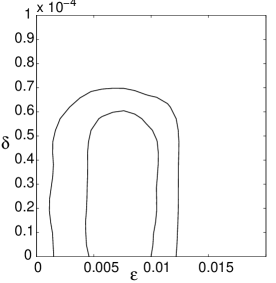
Figure 6: Likelihood plot for allowed values of the slow-roll parameter $\epsilon$ and the inverse-triad correction $\delta$. Observations are consistent with $\delta=0$ and provide an upper bound $\delta<10^{-4}$ [22].

Inverse-triad corrections, depending on the microscopic discreteness scale of a state in relation to the Planck length, are the main correction in sub-Planckian curvature regimes. Closer to the big bang, where the Planck density looms, all corrections, including holonomy effects, are important. Many surprising consequences have been explored in models of loop quantum cosmology [26, 27].

Discreteness means that the wave function of the universe is subject to a difference equation [28, 29],

$$C_{+}(\mu)\psi_{\mu+1}-C_{0}(\mu)\psi_{\mu}+C_{-}(\mu)\psi_{\mu-1}=\hat{H}_{{\rm matter}}(\mu)\psi_{\mu}$$ (12)

with wave functions in the triad representation, depending on flux eigenvalues $\mu\in{\mathbb{R}}$. Following the recurrence, a state is extended uniquely through the classical singularity at $\mu=0$. The singularity is resolved by this mechanism of quantum hyperbolicity [30]. In the deep quantum regime, holonomy corrections and dynamical quantum effects are strong and it is difficult to find an intuitive geometrical picture for the resolution mechanism. Fortunately, some properties can be seen in solvable, harmonic models [31]: the state bounces, reaching a non-zero minimal volume close to the Planck density [32]. This consequence is realized in a special model in which no quantum back-reaction occurs, a flat isotropic model with a free massless scalar. Approximately, the same behavior is realized for models with curvature or small matter masses and self-interactions, but the scenario remains to be confirmed under more general situations [33, 34].

Even though the singularity is resolved, some features demonstrate that space-time, if it even exists in a meaningful form in those extremes, behaves in surprising ways. One of these features is cosmic forgetfulness [35, 36], addressing the question of how much pre-big bang information can be recovered after a state has moved through a resolved classical singularity. Fig. 7 shows sample solutions, the spread around the central lines indicating quantum fluctuations. Different fluctuations can be realized before and after the high-density phase, quantitatively expressed by a squeezing parameter of states [37].

Figure 7: Dynamical wave functions illustrated by their expectation values (central lines) and fluctuations (spreads). The expectation value always bounces at some minimal volume $V$ in this harmonic holonomy-modified model, but fluctuations on the two sides can differ in significant ways.

In more detail, the ratio of volume fluctuations $\Delta V$ at late and early times $t$ is bounded by

$$\left|1-\frac{\Delta V_{t\to-\infty}}{\Delta V_{t\to\infty}}\right|\stackrel{{\scriptstyle\displaystyle<}}{{\sim}}\frac{\Delta H_{\rm matter}/\langle\hat{H}_{\rm matter}\rangle}{(\Delta V/\langle\hat{V}\rangle)_{t\to\infty}}\,,$$ (13)

derived with semiclassical techniques and dynamical coherent states [37, 36, 38]. The right-hand side of this inequality is typically large: the validity of quantum field theory on curved space-time at $t\to\infty$ indicates that matter-energy fluctuations are much larger than geometry fluctuations. The ratio $\Delta V_{t\to-\infty}/{\Delta V_{t\to\infty}}$, and evolutionary aspects influenced by it, remains largely unconstrained, even if the classical singularity can be resolved.

Space-time at and before the big bang is not necessarily classical, even if isotropic models remain well-defined. Additional information about space-time can be gained from the hypersurface-deformation algebra, now evaluated with holonomy corrections for strong-curvature regimes. Preliminary results in different models [14, 39, 40, 1] (taking into account partial holonomy effects) indicate that the algebra is again deformed:

$$[S(\vec{w}_{1}),S(\vec{w}_{2})] = S({\cal L}_{\vec{w}_{2}}\vec{w}_{1})$$ (14)

$${}[T_{\beta}(N),S(\vec{w})] = T_{\beta}(\vec{w}\cdot\vec{\nabla}N)$$ (15)

$${}[T_{\beta}(N_{1}),T_{\beta}(N_{2})] = S(\beta(N_{1}\vec{\nabla}N_{2}-N_{2}\vec{\nabla}N_{1}))$$ (16)

with a function $\beta$ depending on $\raisebox{-4.2679pt}{$\stackrel{{\scriptstyle\textstyle A}}{{\scriptscriptstyle\rightarrow}}$}{}_{i}$, or on curvature. In contrast to inverse-triad corrections, holonomy corrections can result in $\beta<0$, which they do at high density (the “bounce”). In constructions such as Fig. 2, a velocity in one direction would imply motion in the opposite direction, rather intransigent behavior. More meaningfully, one can interpret the phenomenon as signature change [1]: Euclidean 4-dimensional space has a hypersurface-deformation algebra with $\beta=-1$. What appears as a “bounce” in simple isotropic models is not a bounce at all; there is no evolution and no fully deterministic relation between pre- and post-big bang states.

Loop quantum gravity implies radical modifications at Planckian densities, with Euclidean space instead of space-time. There is no propagation of structure from collapse to expansion, as assumed in bounce models. Instead, loop quantum cosmology shows a non-singular beginning of the Lorentzian phase, when the diluting density falls sufficiently below the Planck density. Such a place, nonsingular and yet unprecedented, is natural for posing initial conditions, for instance for an inflaton state. We obtain a mixture of linear and cyclic models. On less extreme scales, loop quantum gravity implies space-time, but with modified structures, allowing quantum-gravity corrections more significant than higher-curvature terms. Inverse-triad corrections are not extremely far from testability; loop quantum gravity is falsifiable.

This work was supported in part by NSF grant PHY0748336.

References:

References

- [1] Bojowald M and Paily G M (Preprint arXiv:1112.1899)
- [2] Dirac P A M 1958 Proc. Roy. Soc. A 246 333–343
- [3] Hojman S A, Kuchař K and Teitelboim C 1976 Ann. Phys. (New York) 96 88–135
- [4] Kuchař K V 1974 J. Math. Phys. 15 708–715
- [5] Bojowald M 2010 Canonical Gravity and Applications: Cosmology, Black Holes, and Quantum Gravity (Cambridge: Cambridge University Press)
- [6] Rovelli C and Smolin L 1995 Nucl. Phys. B 442 593–619, erratum: Nucl. Phys. B 456 753 (Preprint gr-qc/9411005)
- [7] Ashtekar A and Lewandowski J 1997 Class. Quantum Grav. 14 A55–A82 (Preprint gr-qc/9602046)
- [8] Thiemann T 1998 Class. Quantum Grav. 15 839–873 (Preprint gr-qc/9606089)
- [9] Thiemann T 1998 Class. Quantum Grav. 15 1281–1314 (Preprint gr-qc/9705019)
- [10] Bojowald M 2001 Phys. Rev. D 64 084018 (Preprint gr-qc/0105067)
- [11] Bojowald M, Hernández H, Kagan M and Skirzewski A 2007 Phys. Rev. D 75 064022 (Preprint gr-qc/0611112)
- [12] Bojowald M, Calcagni G and Tsujikawa S 2001 JCAP 11 046 (Preprint arXiv:1107.1540)
- [13] Bojowald M, Hossain G, Kagan M and Shankaranarayanan S 2008 Phys. Rev. D 78 063547 (Preprint arXiv:0806.3929)
- [14] Reyes J D 2009 Spherically Symmetric Loop Quantum Gravity: Connections to 2-Dimensional Models and Applications to Gravitational Collapse Ph.D. thesis The Pennsylvania State University
- [15] Bojowald M, Reyes J D and Tibrewala R 2009 Phys. Rev. D 80 084002 (Preprint arXiv:0906.4767)
- [16] Kreienbuehl A, Husain V and Seahra S S 2012 Class. Quantum Grav. 29 095008 (Preprint arXiv:1011.2381)
- [17] Kreienbuehl A, Husain V and Seahra S S (Preprint arXiv:1109.3158)
- [18] Henderson A, Laddha A and Tomlin C (Preprint arXiv:1204.0211)
- [19] Bojowald M, Paily G M, Reyes J D and Tibrewala R 2011 Class. Quantum Grav. 28 185006 (Preprint arXiv:1105.1340)
- [20] Bojowald M, Hossain G, Kagan M and Shankaranarayanan S 2009 Phys. Rev. D 79 043505 (Preprint arXiv:0811.1572)
- [21] Bojowald M and Calcagni G 2011 JCAP 1103 032 (Preprint arXiv:1011.2779)
- [22] Bojowald M, Calcagni G and Tsujikawa S 2011 Phys. Rev. Lett. 107 211302 (Preprint arXiv:1101.5391)
- [23] Barrau A and Grain J 2009 Phys. Rev. Lett. 102 081301 (Preprint arXiv:0902.0145)
- [24] Grain J, Cailleteau T, Barrau A and Gorecki A 2010 Phys. Rev. D 81 024040 (Preprint arXiv:0910.2892)
- [25] Mielczarek J and Szydłowski M 2007 Phys. Lett. B 657 20–26 (Preprint arXiv:0705.4449)
- [26] Bojowald M 2008 Living Rev. Relativity 11 4 http://www.livingreviews.org/lrr-2008-4 (Preprint gr-qc/0601085)
- [27] Bojowald M 2011 Quantum Cosmology: A Fundamental Theory of the Universe (New York: Springer)
- [28] Bojowald M 2001 Phys. Rev. Lett. 86 5227–5230 (Preprint gr-qc/0102069)
- [29] Bojowald M 2002 Class. Quantum Grav. 19 2717–2741 (Preprint gr-qc/0202077)
- [30] Bojowald M 2007 AIP Conf. Proc. 910 294–333 (Preprint gr-qc/0702144)
- [31] Bojowald M 2007 Phys. Rev. D 75 081301(R) (Preprint gr-qc/0608100)
- [32] Ashtekar A, Pawlowski T and Singh P 2006 Phys. Rev. Lett. 96 141301 (Preprint gr-qc/0602086)
- [33] Bojowald M 2008 Gen. Rel. Grav. 40 2659–2683 (Preprint arXiv:0801.4001)
- [34] Bojowald M 2008 Phys. Rev. Lett. 100 221301 (Preprint arXiv:0805.1192)
- [35] Bojowald M 2007 Nature Physics 3 523–525
- [36] Bojowald M 2008 Proc. Roy. Soc. A 464 2135–2150 (Preprint arXiv:0710.4919)
- [37] Bojowald M 2007 Phys. Rev. D 75 123512 (Preprint gr-qc/0703144)
- [38] Kaminski W and Pawlowski T 2010 Phys. Rev. D 81 084027 (Preprint arXiv:1001.2663)
- [39] Perez A and Pranzetti D 2010 Class. Quantum Grav. 27 145009 (Preprint arXiv:1001.3292)
- [40] Cailleteau T, Mielczarek J, Barrau A and Grain J (Preprint arXiv:1111.3535)