Likelihood-Free Cosmological Inference with Type Ia Supernovae: Approximate Bayesian Computation for a Complete Treatment of Uncertainty

Abstract

Cosmological inference becomes increasingly difficult when complex data-generating processes cannot be modeled by simple probability distributions. With the ever-increasing size of data sets in cosmology, there is increasing burden placed on adequate modeling; systematic errors in the model will dominate where previously these were swamped by statistical errors. For example, Gaussian distributions are an insufficient representation for errors in quantities like photometric redshifts. Likewise, it can be difficult to quantify analytically the distribution of errors that are introduced in complex fitting codes. Without a simple form for these distributions, it becomes difficult to accurately construct a likelihood function for the data as a function of parameters of interest. Approximate Bayesian computation (ABC) provides a means of probing the posterior distribution when direct calculation of a sufficiently accurate likelihood is intractable. ABC allows one to bypass direct calculation of the likelihood but instead relies upon the ability to simulate the forward process that generated the data. These simulations can naturally incorporate priors placed on nuisance parameters, and hence these can be marginalized in a natural way. We present and discuss ABC methods in the context of supernova cosmology using data from the SDSS-II Supernova Survey. Assuming a flat cosmology and constant dark energy equation of state we demonstrate that ABC can recover an accurate posterior distribution. Finally we show that ABC can still produce an accurate posterior distribution when we contaminate the sample with Type IIP supernovae.

1 Introduction

Since the discovery of the accelerated expansion of our universe (Riess et al., 1998; Perlmutter et al., 1999), the quality of Type Ia supernova (SN Ia) data sets has improved and the quantity has grown to thousands through individual efforts with the Hubble Space Telescope (Knop et al., 2003; Riess et al., 2004; Amanullah et al., 2010) and surveys such as the Supernova Legacy Survey (Astier et al., 2006; Conley et al., 2011), the ESSENCE Supernova Survey (Miknaitis et al., 2007; Wood-Vasey et al., 2007), the CfA Supernova group (Hicken et al., 2009, 2012), the Carnegie Supernova Project (Contreras et al., 2010; Stritzinger et al., 2011), the Sloan Digital Sky Survey-II (Lampeitl et al., 2010), and the Lick Observatory Supernova Search (Ganeshalingam et al., 2010). Additional current and near-future surveys such as the Palomar Transient Factory (Law et al., 2009), the Panoramic Survey Telescope and Rapid Response System (Pan-STARRS), SkyMapper, and the Dark Energy Survey will increase the sample by another order of magnitude with the goal of obtaining tighter constraints on the nature of dark energy. The Large Synoptic Survey Telescope (LSST) anticipates observing hundreds of thousands of well-measured Type Ia supernovae (SNe Ia) (LSST Science Collaborations et al., 2009).

In this new regime of large numbers of SNe Ia the weaknesses and limitations of our current $\chi^{2}$ likelihood approach to estimating cosmological parameters are becoming apparent. For example, with limited spectroscopic follow-up, we must rely on light-curve classification codes and photometric redshift tools to maximize the scientific potential of SN Ia cosmology with LSST and near-future surveys. These two crucial steps alone introduce a nontrivial component to our probability models from which we construct the likelihood. Additionally, there are significant systematic uncertainties including errors from calibration, survey design and cadence, host galaxy subtraction and intrinsic dust, population evolution, gravitational lensing, and peculiar velocities. All of these uncertainties contribute to a probability model which simply cannot be accurately described by a multivariate normal distribution.

In this paper we describe how the statistical technique of Approximate Bayesian Computation (ABC) can be used to overcome these challenges and explore the space of cosmological parameters in the face of non-Gaussian distributions of systematic uncertainties, complicated functional priors, and large data sets. We encourage the reader to read the recent paper by Cameron & Pettitt (2012) for an introduction to and application of ABC in the context of galaxy evolution. We here focus on supernova cosmology, but ABC has applicability in a wide range of forward-modeling problems in astrophysics and cosmology.

1.1 Classical Estimation of Cosmological Parameters from SN Ia Data

Cosmological inference with SNe Ia is a classical statistical estimation problem. We have data, our set of supernova light-curve observations, and we seek to infer something about the universe in which we live. It is standard in cosmology to adopt a Bayesian approach to inference. To clarify our basic conceptual and notational framework, we review Bayes theorem, a simple identity which relates the posterior probability distribution–the probability of a set of model parameters given the data–to the probability of the data given the model, the likelihood. More precisely, the posterior probability distribution is derived as

$$\pi({\theta}\hskip 0.72229pt|\>{\bf x})=\frac{p({\bf x}\hskip 0.72229pt|\>{\theta})\pi({\theta})}{p({\bf x})}$$ (1)

where $p({\bf x}\hskip 0.72229pt|\>\theta)$ is the likelihood, $\pi({\theta})$ is the prior on the vector of model parameters $\theta$, and $p({\bf x})$ is the marginal probability of the data ${\bf x}$ ($p({\bf x})=\int_{{\Theta}}p({\bf x}\hskip 0.72229pt|\>\theta)\pi(\theta)d{\theta}$). The Bayesian framework is powerful in that it allows evidence and experience to modify the prior. The approach is challenging, however, in that standard computation methods rely upon full specification of the likelihood $p({\bf x}\hskip 0.72229pt|\>\theta)$; this can be challenging in applications of interest.

For example, consider a cosmological model for which the distance modulus can be written as $\mu_{\rm model}=\mu_{\rm model}(\Omega_{M},\Omega_{\Lambda},w,z)$. If we assume that each measured $\mu$ has a probability distribution function (PDF) described by a Gaussian with standard deviation $\sigma$ we can write the likelihood for a single observation as

$$p(\mu_{i},z_{i}|\Omega_{M},\Omega_{\Lambda},w)\propto\exp{\left[-\frac{(\mu_{i}-\mu_{\rm model}(z_{i},\Omega_{M},\Omega_{\Lambda},w))^{2}}{2\sigma_{i}^{2}}\right]}.$$ (2)

If the distance observations are independent after calibration such that there are no correlated uncertainties we can simply multiply the likelihood of each observation together. By taking the logarithm, we can write a more convenient form of the likelihood as follows

$$-2\ln{(p(\mu,z|\Omega_{M},\Omega_{\Lambda},w))}=K+\sum_{i=1}^{N}\frac{(\mu_{i}-\mu_{\rm model}(z_{i},\Omega_{M},\Omega_{\Lambda},w))^{2}}{\sigma_{i}^{2}},$$ (3)

where $K$ is an unimportant constant, giving us the familiar $\chi^{2}$ statistic. Note that the use of this form of the likelihood function and $\chi^{2}$ statistic is based on the assumption of independent data with normally distributed uncertainties.

Traditionally when making cosmological inference with SNe Ia one calculates the $\chi^{2}$ statistic (Conley et al., 2011; Kessler et al., 2009a; Wood-Vasey et al., 2007; Astier et al., 2006; Riess et al., 2004). One method of including systematic uncertainties in such a framework is to use the “quadrature” method, accurately named by Conley et al. (2011). Systematic errors which are not redshift dependent and add scatter to the overall Hubble diagram are added in quadrature to the statistical uncertainties. For other sources of systematic uncertainty it is typical to perform the analysis with and without including the systematic effect on the data. The difference in inferred cosmological parameter is then a measure of the systematic uncertainty. All systematic effects are then added in quadrature as the quoted total systematic uncertainty. This method has been used in recent cosmological analyses by Kessler et al. (2009a), Wood-Vasey et al. (2007), and Astier et al. (2006). It has the advantage of being simple to implement but the disadvantage of missing correlations between systematic uncertainties, not producing the full likelihood, and could be inappropriate for asymmetric error distributions (Barlow, 2003). One also has the difficult task of estimating the size of the systematic uncertainty and implementing its effect in the analysis.

Conley et al. (2011) presented a more thorough approach to incorporating systematic uncertainties into a $\chi^{2}$ analysis using a covariance matrix. By implementing a covariance matrix one can drop the assumption of independent data in Eq. 3. The covariance matrix can be decomposed into a diagonal, statistical component and two off-diagonal matrices which include statistical and systematic uncertainty. These off-diagonal covariance matrices include uncertainties from, e.g., uncertainty in the supernova model which is statistical in nature but could be correlated between different SNe Ia and uncertainty in zero points which would systematically affect all SNe Ia. Kowalski et al. (2008) and Amanullah et al. (2010) present similar methods which are approximations to Conley et al. (2011)’s covariance matrix approach. However, the overall approach must be modified for uncertainties due to, e.g., type contamination and Malmquist bias. They have the effect of adding or removing supernovae from the sample which is difficult to represent in a covariance matrix. For systematic effects such as these the field of supernova cosmology is moving toward calculating the corrections to the data using artificial SNe Ia generated from Monte Carlo simulations.

Bayesian inference becomes increasingly difficult as we depart from normal error distributions or when the likelihood function is not analytically or computationally tractable. Direct calculation of the likelihood may involve many integrations over systematic uncertainties, nuisance parameters, and latent variables. These integrations can make the use of standard Markov Chain Monte Carlo (MCMC) techniques very challenging and computational expensive. It may also be incredibly difficult to construct an analytic probability model over which to marginalize.

ABC allows one to bypass direct calculation of the likelihood by simulating data from the posterior distribution. The posterior distribution is then constructed from the model parameters necessary to simulate data which resemble the observed data. By incorporating into the simulation all of the statistical and systematic uncertainties for which we have models and priors, the simulation knows about the complicated probability model even thought the observer may not be able to have the model written out as a set of equations or numerical integrals. By simulating many realistic datasets one can marginalize over the nuisance parameters and systematic uncertainties such that high-dimensional marginalization problems, as in population genetics for which ABC techniques were first developed, are now computationally feasible. ABC is a consistent framework to incorporate systematic uncertainties with the cosmological model and more clearly defines what it means to use Monte Carlo simulations of artificial SNe Ia to quantify systematic uncertainty.

We begin in § 2 by motivating the general problem and discussing the breakdown of current cosmological inference methods using a simple example. In § 3 we outline three separate ABC algorithms and discuss their merits. To provide the reader with an introductory example of using ABC, we then illustrate how one might perform cosmological inference with Sequential Monte Carlo (SMC) ABC using the simple model discussed in § 2. In § 4 we present a more sophisticated analysis using SNe Ia from the Sloan Digital Sky Survey-II (SDSS-II) Supernova Survey and demonstrate how one might perform cosmological inference with a tool like the SuperNova ANAlysis (SNANA) (Kessler et al., 2009b) software using SMC ABC techniques. We compare our results to the cosmological analysis performed in Kessler et al. (2009a) using statistical errors only. At the end of this section we show that ABC can recover the full posterior distribution when we contaminate the data with simulated Type IIP supernovae. We discuss directions for future work in § 5 and conclude in § 6.

2 General Problem Formulation

Here we establish notation that we will use in discussing the SN Ia inference problem. Below we explain how this framework could be extended to other cosmological inference challenges. Let $\mu_{i}$ be the measured distance modulus of the $i^{th}$ SN Ia in our sample, $\tau_{i}$ be its true distance modulus, $z_{i}$ be the estimated redshift, and $\theta$ be the vector of cosmological parameters. We will use bold faced variables to indicate a set of $n$ supernovae, e.g., ${\bf z}=\{z_{1},...,z_{n}\}$. Here, we stress that the “estimated redshift” will be, in practice, the redshift as estimated from photometry, i.e., the photometric redshift.

The underlying objective is to determine the posterior of the cosmological parameters $\theta$ given the observed data $({\bm{\mu}},{\bf z})$. There are two natural analytical routes, both of which lead to the same challenges. The first route is to note that the posterior of $\theta$ can be decomposed as

$$\pi(\theta\hskip 0.72229pt|\>{\bm{\mu}},{\bf z})=Kp({\bm{\mu}}\hskip 0.72229pt|\>\theta,{\bf z})\pi(\theta,{\bf z})$$ (4)

where $K$ is a constant that does not depend on $\theta$ and

$$p({\bm{\mu}}\hskip 0.72229pt|\>\theta,{\bf z})\pi(\theta,{\bf z}) = \left[\int p({\bm{\mu}}\hskip 0.72229pt|\>\theta,{\bf z},\bm{\tau})\>p({\bm{\tau}}\hskip 0.72229pt|\>\theta,{\bf z})\>d{\bm{\tau}}\right]\pi(\theta,{\bf z})$$ (5)

$$= \left[\int p({\bm{\mu}}\hskip 0.72229pt|\>\theta,{\bm{\tau}})\>p({\bm{\tau}}\hskip 0.72229pt|\>\theta,{\bf z})\>d{\bm{\tau}}\right]\pi(\theta,{\bf z}).$$ (6)

Note that in this last step, the density of ${\bm{\mu}}$ conditional on $\theta$ and ${\bf z}$ is replaced with the density of ${\bm{\mu}}$ conditional only on $\theta$. Here we are assuming that ${\bm{\mu}}$ and ${\bf z}$ are independent given ${\bm{\tau}}$: Once $\bm{\tau}$ is known, the information in ${\bf z}$ does not affect the distribution of ${\bm{\mu}}$. We note that this assumption is not true if one is using the photometric redshift determined from the supernova light curve.

We could pose this problem in general statistical terms as follows. Assume that ${\bm{\mu}}=\left\{\mu_{1},\mu_{2},\ldots,\mu_{n}\right\}$ are random variables such that the distribution of $\mu_{i}$ is determined by parameters $\theta$ and $\tau_{i}$. Here, $\theta$ represents the unknown parameters common to the $\mu_{i}$ while $\tau_{i}$ are the object-specific parameters. We further assume the existence of additional data, denoted $z_{i}$, which have the property that $\mu_{i}$ and $z_{i}$ are independent conditional on $\tau_{i}$. The quantities $z_{i}$ can be thought of as properties that help in the estimation of $\tau_{i}$, but would not be useful for estimating $\theta$ if $\tau_{i}$ were known.

Note that each of $\mu_{i}$ and $\tau_{i}$ could be vectors. For example, in Mandel et al. (2011), $\mu_{i}$ stores the full observed light curve of the supernova and $\tau_{i}$ comprises not only the true distance modulus, but also parameters that capture the effect of extinction and dust and that define the true, underlying light curve. As mentioned above, these have the property that, if $\tau_{i}$ were known, $z_{i}$ would not provide useful additional information for the estimation of $\theta$.

The second route is to rewrite the posterior as

$$\pi(\theta\hskip 0.72229pt|\>{\bm{\mu}},{\bf z})=\int p(\theta,{\bm{\tau}}\hskip 0.72229pt|\>{\bm{\mu}},{\bf z})\>d{\bm{\tau}}$$ (7)

and then rely upon the fact that, as derived above,

$$p(\theta,{\bm{\tau}}\hskip 0.72229pt|\>{\bm{\mu}},{\bf z})=p({\bm{\mu}}\hskip 0.72229pt|\>\theta,{\bm{\tau}})\>p({\bm{\tau}}\hskip 0.72229pt|\>\theta,{\bf z})\pi(\theta,{\bf z})$$ (8)

to construct a hierarchical Bayesian model for the unknown “parameters” which now consist of both $\theta$ and $\bm{\tau}$. To analytically obtain the posterior in terms of only $\theta$, one must integrate over $\bm{\tau}$, i.e., find

$$\int p({\bm{\mu}}\hskip 0.72229pt|\>\theta,{\bm{\tau}})\>p({\bm{\tau}}\hskip 0.72229pt|\>\theta,{\bf z})\>d{\bm{\tau}}.$$ (9)

This is exactly the form of the challenging integral that was confronted above in Equation (6). One can often justify further conditional independence assumptions and write

$$\int p({\bm{\mu}}\hskip 0.72229pt|\>\theta,{\bm{\tau}})\>p({\bm{\tau}}\hskip 0.72229pt|\>\theta,{\bf z})\>d{\bm{\tau}}\> = \int\prod_{i=1}^{n}p(\mu_{i}\hskip 0.72229pt|\>\theta,\tau_{i})\>p(\tau_{i}\hskip 0.72229pt|\>\theta,z_{i})\>d{\bm{\tau}}$$ (10)

$$= \>\prod_{i=1}^{n}\int p(\mu_{i}\hskip 0.72229pt|\>\theta,\tau_{i})\>p(\tau_{i}\hskip 0.72229pt|\>\theta,z_{i})\>d\tau_{i}.$$ (11)

Still, the computational feasibility of using analytical approaches to finding the posterior for $\theta$ will depend on the form of

$$p(\mu_{i}\hskip 0.72229pt|\>\theta,z_{i})=\int p(\mu_{i}\hskip 0.72229pt|\>\theta,\tau_{i})\>p(\tau_{i}\hskip 0.72229pt|\>\theta,z_{i})\>d\tau_{i}.\\$$ (12)

In practice, the complex nature of photometric redshift estimators will yield a complex form for the distribution $p(\tau_{i}\hskip 0.72229pt|\>\theta,z_{i})$.

An alternative is to adopt the “second route” described above but instead utilize MCMC methods to simulate from the posterior for both $(\theta,\tau)$. This is the approach taken in Mandel et al. (2011). This avoids the integral over $\tau_{i}$, but it is still apparent that practical implementation of analytical or MCMC methods when $n$ is large (and hence $\bm{\tau}$ is of high dimension) forces one to make choices for $p(\mu_{i}\hskip 0.72229pt|\>\theta,\tau_{i})$ and $p(\tau_{i}\hskip 0.72229pt|\>\theta,z_{i})$ which may not be realistic. Unfortunately, as $n$ gets large, even small mistakes in the specification of these densities could lead to significant biases in the estimates of the parameters. This is one of the fundamental challenges facing cosmology as we are presented with ever-larger data sets. In what follows we will develop an example that illustrates this point.

2.1 A Simple Example

To begin, note that in the present example $\mu_{i}$ is the measured distance modulus, $z_{i}$ is the measured redshift, $\tau_{i}$ is the true distance modulus, and $\theta$ represent the set of cosmological parameters. We ignore for the moment all parameters which affect the measured distance modulus except $z_{i}$ and $\theta$. The measured redshift $z_{i}$ may differ from the true redshift of the supernova, which we will denote $\zeta_{i}$. Consider the following three scenarios:

1. $z_{i}=\zeta_{i}$, i.e., the redshift is known exactly. In this case, and under our simplifying assumptions, we know exactly the value of $\tau_{i}$, and hence the “density” $p(\tau_{i}\hskip 0.72229pt|\>\theta,z_{i})$ is a delta function at this known value.

2. The redshift is observed with some normal error. We model $\zeta_{i}$ with a Gaussian PDF with mean $z_{i}$ and variance $\sigma_{z,i}^{2}$. In this case we can apply the so-called “delta method” and state that $p(\tau_{i}\hskip 0.72229pt|\>\theta,z_{i})$ is approximately Gaussian with mean $\mu(z_{i},\theta)$. This scenario is analogous to measuring a spectroscopic redshift with a small error such that a Gaussian approximation for the PDF of $\zeta_{i}$ is sufficient or a photometric redshift which has a PDF which can be modeled well by a Gaussian.

3. $z_{i}$ is observed with some complicated uncertainty. The PDF is not described by a simple function although $p(\tau_{i}\hskip 0.72229pt|\>\theta,z_{i})$ may be estimated using observed data. This is the case for most photometric redshifts.

Of course, the first case is unrealistic. In order to demonstrate the pitfalls of making unwarranted assumptions regarding the likelihood function, we will first focus on the second case, in particular assume that $p(\tau_{i}\hskip 0.72229pt|\>\theta,z_{i})$ is a Gaussian density with mean $\mu(z_{i},\theta)$. The rationale for this approximation relies on the assumption that the true redshift $\zeta_{i}$ also has a Gaussian distribution, in this case with mean $z_{i}$ and variance $\sigma^{2}_{z,i}$. The true distance modulus is $\tau_{i}=\mu(\zeta_{i},\theta)$, so, using the standard linear approximation, we can argue that $\tau_{i}$ is approximately normal with mean $\mu(z_{i},\theta)$ and variance

$$\left(\sigma^{z}_{\mu,i}\right)^{2}=\left[\frac{\partial\mu(z_{i},\theta)}{\partial z_{i}}\right]^{2}\sigma^{2}_{z,i}.$$ (13)

Then, the observed distance modulus can be modeled as the true distance modulus plus some additional Gaussian error; this is taken to have mean zero and variance $\left(\sigma_{\mu,i}\right)^{2}$. In a real-life application this variance includes uncertainty from the observed intrinsic dispersion in distance modulus and uncertainty from fitting the light curve.

This is the current approach in most cosmological analyses where one has spectroscopic redshifts for each SN Ia (Conley et al., 2011; Kessler et al., 2009a; Wood-Vasey et al., 2007; Astier et al., 2006). The uncertainty in redshift is transferred to the uncertainty in measured distance modulus and one can find an analytic solution to Eq. 12 by noting that the integral is simply the convolution of two normal densities. Hence the result of Eq. 12 is another normal density, but now with mean $\mu(z_{i},\theta)$ and variance $\left(\sigma^{z}_{\mu,i}\right)^{2}+\left(\sigma_{\mu,i}\right)^{2}$. This approach is also possible for larger uncertainties like those from photometric redshifts, but the concern becomes the fact that the linear approximation utilized does not extend to larger ranges of redshift. In what follows we examine the consequences of making this Gaussian assumption for photometric redshift uncertainties when the approximation is not valid, i.e., we treat scenario 3 as if it were scenario 2.

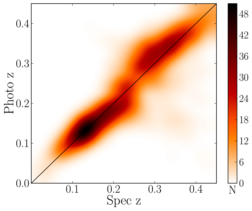
Figure 1: Photometric vs. spectroscopic redshift for 1744 simulated SNe Ia using SNANA and smoothed with a Gaussian kernel. Note the complex structure and asymmetry about the one-to-one line indicating departures from Gaussianity. This sample is used to represent a realistic joint distribution between the spectroscopic and photometric redshifts.

Fig. 1 shows the photometric versus spectroscopic redshift for a sample of 1744 SNe Ia generated using SNANA version v9_32 and smoothed with a Gaussian kernel. To make this figure, light curves were simulated and fit from the MLCS2k2 model (Jha et al., 2007) as described in Section 4 with the following changes; we fix the cosmology to $\Omega_{\Lambda}=0.73$, $\Omega_{M}=0.27$ and $w=-1$, and we estimate photometric redshifts when we fit the light curves without using a host galaxy photo-z prior. We use this sample to represent a realistic joint distribution between the spectroscopic and photometric redshifts. We further assume that the spectroscopic redshift is equal to the true redshift $\zeta=z^{\rm spec}$ and the observed redshift is the photometric redshift $z=z^{\rm phot}$.

Fig. 2 shows three cross-sections of the joint distribution of spectroscopic and photometric redshifts, comparing the photometric redshift distribution with the assumed Gaussian PDF. Our proposed model assumes that the horizontal cross-section of this distribution at $z^{\rm phot}$ is Gaussian with mean equal to $z^{\rm spec}$. This figure demonstrates that the Gaussian approximation to the distribution of $z^{\rm spec}$ is not terrible. Further, under this Gaussian approximation $\mu(z^{\rm phot}_{i},\theta)$ should be approximately normal with mean $\tau_{i}$, i.e., under the linear approximation the distance modulus estimated using the photometric redshift has mean equal to the true distance modulus. Fig. 3 uses boxplots to show the distribution of $\tau_{i}-\mu(z^{\rm phot}_{i},\theta)$ at various values of $z^{\rm phot}$ for the simulated data. This plot reveals that there are significant deviations from the expected difference of zero.

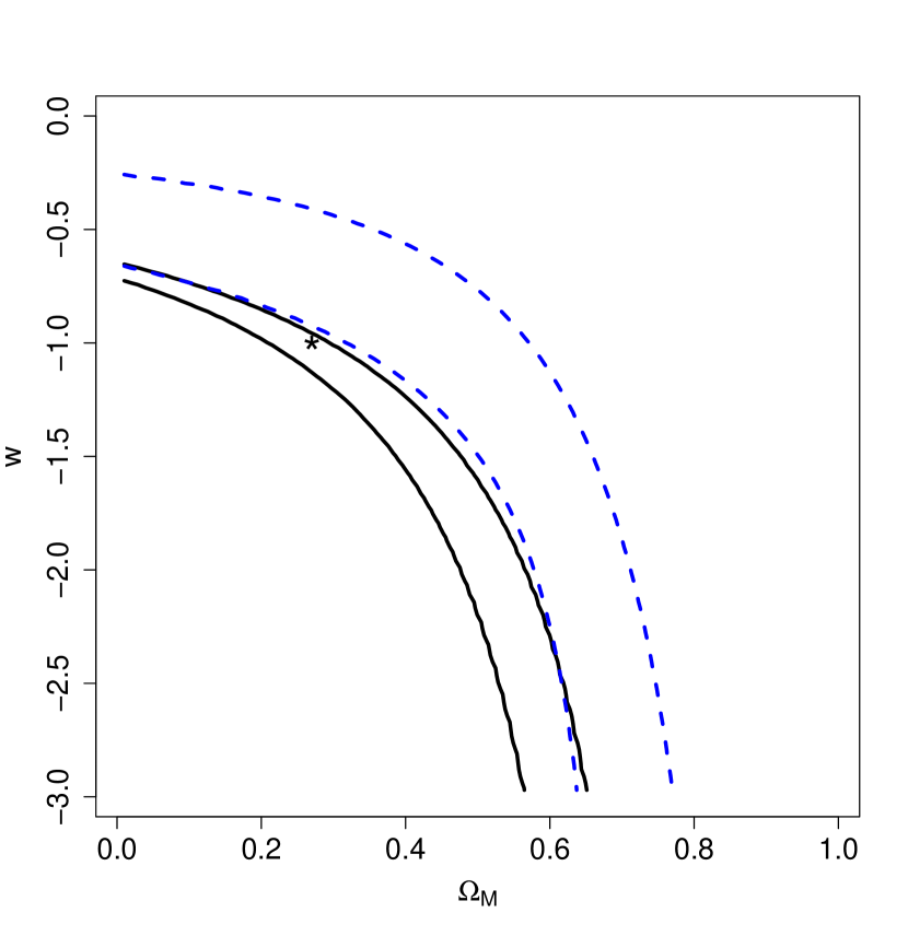
Figure 4: Comparison between the 95% credible regions for a simulated set of supernova formed by taking two approaches: (1) where the true redshift is known (black-solid line) and (2) where the approximation described in Section 2.1 is utilized (blue-dashed line). The star is at the true value of the parameters used in the simulation. The increased width of the confidence region is natural, given the use of photometric redshifts instead of spectroscopic redshifts, but the bias is a result of the inadequacy of the assumed Gaussian model.

The effect of this bias is made clear in Fig. 4. This figure shows the 95% credible region as constructed by two different methods, which will be described below. In both cases, the data set utilized is the same. To construct this data set we simulated a sample of 200 SNe Ia by drawing with replacement from the $(z^{\rm spec},z^{\rm phot})$ sample shown in Fig. 1. We then calculated $\tau=\mu(z^{\rm spec},\theta)$, where $\theta$ consists of $w=-1$ and $\Omega_{M}=0.27$ and assumed a flat universe. Finally the observed distance modulus $\mu$ is constructed by adding mean-zero Gaussian error onto $\tau$ with variance $\sigma_{\mu,i}^{2}=0.04$. The posterior for $\theta$ is found for this dataset in two ways, and the 95% credible region is displayed for each.

1. The solid line shows the credible region if the posterior is constructed using $z^{\rm spec}$. It will serve as the fiducial reference for comparisons to the other region.

2. The dashed line is the credible region that results from using the approximation described above, i.e., assuming that the observed distance modulus has a Gaussian PDF with variance

   $$\left[\frac{\partial\mu(z^{\rm phot}_{i},\theta)}{\partial z^{\rm phot}_{i}}\right]^{2}\sigma^{2}_{z^{\rm phot},i}\,+\,\sigma^{2}_{\mu,i}.$$ (14)

   The point of emphasis here is that the additional uncertainty in the redshift is now taken into account and reflected in the extra width of the region as compared to the solid region. The shift from the solid region to the dashed region is the result of a bias.

The bias shown in Fig. 4 is much like the attenuation bias that results from inappropriately taking into account the errors in the predictor variables in a regression setting: simply adding more error into the response will not adequately account for this additional error. There are methods for dealing with this additional error, but these are not practical in this setting because of another fundamental challenge: the variance of the error in redshift cannot be assumed to be constant, it needs to be modeled as a function of redshift. This heteroskedastic error introduces significant obstacles to any method that would seek to “back out” its effect on the estimates. In the next section we will instead consider approaches that exploit our ability to model and/or simulate the forward process that generated the data, and hence allow us to incorporate in a natural way the errors due to the use of photometric redshifts.

3 Approximate Bayesian Computation

ABC methods simulate observations from the posterior distribution via algorithms that bypass direct calculation of the likelihood. This is done by drawing model parameters from some distribution, generating simulated data based on these model parameters and reducing the simulated data to summary statistics. Summary statistics are measures of the data designed to reduce the dimensionality of the data: they represent the maximum amount of information in the simplest form. Model parameters that generate data sufficiently similar to the observed data are drawn from the posterior distribution. This procedure allows one to simulate the complicated integral in Eq. 12 rather than evaluate it but instead relies upon the ability to simulate the forward process that generated the observed data.

Here we review two classes of ABC algorithms; ABC rejection samplers and adaptive ABC algorithms. The roots of ABC techniques lie in the first class while the goal of adaptive ABC algorithms is to efficiently determine the relevant regions of parameter and probability space to sample from. In this section we will adopt a Bayesian approach and endeavor to determine (approximately) the posterior distribution of model parameters $\theta$ given observed data ${\bf x}$. The posterior is given by

$$\pi(\theta\hskip 0.72229pt|\>{\bf x})=\frac{p({\bf x}\hskip 0.72229pt|\>\theta)\pi(\theta)}{p({\bf x})},$$ (15)

where $p({\bf x}\hskip 0.72229pt|\>\theta)$ is the likelihood function and $p({\bf x})$ is a normalization constant. For a review on ABC algorithms we refer the reader to Marin et al. (2011).

3.1 ABC Rejection Samplers

The basic ABC prescription is best considered for a situation in which the data ${\bf x}$ are discrete:

Rejection Sampler: Discrete Case 1. Draw candidate $\theta^{*}$ from $\pi(\theta)$ 2. Simulate data ${\bf x^{*}}\sim p({\bf x^{*}}\hskip 0.72229pt|\>\theta^{*})$ 3. Accept $\theta^{*}$ if ${\bf x^{*}}={\bf x}$ Repeat these steps until $N$ candidates are accepted.

Under this algorithm, the probability that $\theta^{*}$ is accepted is exactly $\pi(\theta\hskip 0.72229pt|\>{\bf x})$. Hence, it is simple in principle to generate a sample of size $N$ from the posterior distribution. This sample is then used to estimate properties of the posterior distribution such as the 95% credible region.

In practice, however, most data are continuous, and we must instead decide to accept $\theta^{*}$ if ${\bf x^{*}}$ is suitably “close to” ${\bf x}$; hence, a metric or distance $\Delta({\bf x^{*}},{\bf x})$ must be chosen. Under this setup, the accepted parameter vectors $\theta^{*}$ are drawn from the posterior distribution conditioned on the simulated data being sufficiently close to the observed data. More precisely, the result will be a sample from the joint distribution $p({\bf x},\theta\hskip 0.72229pt|\>\Delta({\bf x},{\bf x^{*}})\leq\epsilon)$ where $\epsilon>0$ is a fixed tolerance. If $\epsilon$ is small and one marginalizes over ${\bf x}$, then $p(\theta\hskip 0.72229pt|\>\Delta({\bf x},{\bf x^{*}})\leq\epsilon)$ is a reasonable approximation to $\pi(\theta\hskip 0.72229pt|\>{\bf x})$ (Sisson et al., 2007). Note that if $\epsilon$ is very large the sample will be effectively drawn from the prior. The continuous version of the ABC rejection sampler, introduced by Tavare et al. (1997) and Pritchard et al. (1999), is built upon this idea:

Rejection Sampler: Continuous Case 1. Draw candidate $\theta^{*}$ from $\pi(\theta)$ 2. Simulate data ${\bf x^{*}}\sim p({\bf x^{*}}\hskip 0.72229pt|\>\theta^{*})$ 3. Accept $\theta^{*}$ if $\Delta({\bf x^{*}},{\bf x})\leq\epsilon$ Repeat these steps until $N$ candidates are accepted.

If the data have many dimensions, requiring that $\Delta({\bf x^{*}},{\bf x})\leq\epsilon$ may be impractical. For example, it would be nearly impossible to simulate $10^{3}$ supernovae to within $\epsilon$ of the observed data even with the correct cosmology due to random photometric error, let alone population variance in realizations of stretch and color distribution.

Fu & Li (1997) and Weiss & von Haeseler (1998) improved Step 3 by instead making the comparison between lower-dimensional summaries of the data; here these will be denoted ${s}({\bf x})$, or just ${s}$. The ideal choice for ${s}$ would be a summary statistic that is a sufficient statistic for estimating $\theta$. Technically, a vector ${s}$ is sufficient if $p({\bf x}\hskip 0.72229pt|\>{s},\theta)$ is not a function of $\theta$, and hence the posterior conditioned on ${s}$ is the same as the posterior conditioned on ${\bf x}$, i.e., $\pi(\theta\hskip 0.72229pt|\>{s})=\pi(\theta\hskip 0.72229pt|\>{\bf x})$. Of course, one cannot expect to derive an exactly sufficient statistic when the form of the likelihood is not known. Hence, much current research in ABC is focused on the derivation of approximately sufficient statistics or, more generally, summary statistics that preserve important information regarding the parameters of interest. Blum et al. (2012) provide an excellent overview and comparison of methods for constructing summary statistics. These methods generally fall into two categories: those that sift through a list of candidate summary statistics to find the “best” summary statistic as measured by some optimality criterion, and those that utilize the ability to simulate data sets under different parameter values as part of a process of fitting a regression where the responses are the parameters, and the predictors are the simulated data. This mapping is then used to transform observed summary statistics to parameters. For example, an early such example was Beaumont et al. (2002), who fit local linear regression to simulated parameter values on simulated summary statistics. The regression approach can be justified on theoretical grounds, see Fearnhead & Prangle (2012), and Cameron & Pettitt (2012) used this approach for their astronomical application. In our work, the relatively simple structure of the relationship between the simulated data and the parameters of interest leads to a natural approach to constructing a summary statistic: exploiting the known smooth distance modulus/redshift relationship. In other applications, there will not exist such a simple one-dimensional representation of the data, and these sophisticated approaches must be utilized.

There are advantages to the general ABC rejection sampler approach. Since each accepted parameter represents an independent draw from $p(\theta\hskip 0.72229pt|\>\Delta({s^{*}},{s})\leq\epsilon)$, properties of the posterior distribution are easily estimated from the accepted sample. There are no problems with such estimation due to dependence in the sample. Also, the ABC rejection sampler is simple to code and trivial to parallelize. However, the success of this method depends on how easy it is to simulate data from the model. If the model is complicated or if the acceptance rates are small, then the algorithm can be very expensive or inefficient. A low acceptance rate can be caused by a diffuse prior relative to the posterior or by a poor choice for the summary statistic. It is natural to consider approaches that do not rely upon independent sampling from the prior. In particular, one would anticipate that it would be possible to “learn” from the parameter values that have been accepted in the past to determine where good choices for future candidates $\theta^{*}$.

3.2 Adaptive ABC Algorithms

The aforementioned challenges are the major motivations for the use of MCMC techniques: instead of relying on random draws from a distribution to produce candidates, random walks are taken in parameter space. Marjoram et al. (2003) presented an MCMC version of ABC as follows:

ABC MCMC Initialize $\theta_{i},~{}i=1$ For $i$=1 to $i$=$N$ do: 1. Propose a move to $\theta^{*}$ according to a transition kernel $q(\theta_{i}\rightarrow\theta^{*})$ 2. Simulate ${\bf x^{*}}\sim p({\bf x^{*}}\hskip 0.72229pt|\>\theta^{*})$ 3. Measure ${s^{*}}$ from ${\bf x^{*}}$ 4. If $\Delta({s^{*}},{s})\leq\epsilon$ proceed, else go to Step 1 5. Set $\theta_{i+1}=\theta^{*}$ with probability $$h(\theta_{i},\theta^{*})={\rm min}\left(1,\frac{\pi(\theta^{*})q(\theta_{i}\rightarrow\theta^{*})}{\pi(\theta_{i})q(\theta^{*}\rightarrow\theta_{i})}\right)$$ and otherwise, $\theta_{i+1}=\theta_{i}$ 6. $i=i+1$

Here $q(\theta_{i}\rightarrow\theta^{*})$ is a proposal density, $h(\theta_{i},\theta^{*})$ is the Metropolis–Hastings acceptance probability and $N$ is the chain length. The chain length is determined after meeting some convergence criterion (see, e.g., Cowles & Carlin (1996)). As is proved in Marjoram et al. (2003), the posterior distribution of interest $\pi(\theta\hskip 0.72229pt|\>{\bf x})$ is the stationary distribution of the chain.

The MCMC ABC algorithm can be much more efficient than the ABC rejection sampler, especially when the posterior and prior distributions are very different. This efficiency is gained, however, at the cost of highly correlated $\theta_{i}$. Additionally, the MCMC ABC sampler can become inefficient if it wanders into a region of parameter space with low acceptance probability with a poor perturbation kernel. Successive perturbations have a small chance or being accepted and the chain can get “stuck.” It is worth noting that this algorithm is replacing the likelihood ratio present in standard MCMC techniques with a one or zero based on whether or not $\Delta({s^{*}},{s})\leq\epsilon$. This is a significant loss of resolution in the information that was present in the likelihood ratio.

Sisson et al. (2007) (improved upon by Beaumont et al. (2009)) overcome the inefficiencies of a MCMC ABC algorithm via a method which they term Population Monte Carlo or Sequential Monte Carlo (SMC) ABC. The SMC ABC approach adapts the SMC methods developed in Moral et al. (2006) to ABC. The algorithm learns about the target distribution using a set of weighted random variables that are propagated over iterations, similar to running parallel MCMC algorithms which interact at each iteration. The basic recipe of the SMC ABC algorithm is to initialize $N$ points in parameter space according to $\pi(\theta)$. Points or particles are drawn from this sample, slightly perturbed, and are accepted for the next iteration if they meet the $\epsilon$ criterion. For each iteration, the tolerance $\epsilon$ is decreased, slowly migrating the $N$ particles into the correct region of parameter space when we have reached a pre-specified tolerance threshold.

SMC ABC Fix a decreasing sequence of tolerances $\epsilon=\epsilon_{1},\epsilon_{2},...,\epsilon_{T}$ For the first iteration, $t$=1: For $i$=1 to $i$=$N$ do: 1. Draw $\theta_{i}^{t}$ from $\pi(\theta)$ 2. Simulate ${\bf x}_{i}^{t}\sim p\left({\bf x}_{i}^{t}\hskip 0.72229pt|\>\theta_{i}^{t}\right)$ 3. Measure ${s}^{t}_{i}$ from ${\bf x}_{i}^{t}$ 4. Proceed if $\Delta({s}^{t}_{i},{s})<\epsilon_{t}$, else return to Step 1 5. Set $w_{i}=1/N$ 6. $i=i+1$ Take $\tau_{t+1}^{2}$ equal to twice the weighted variance of the set $\{\theta_{i}^{t}:i=1,...,N\}$. For $t$=2 to $t$=$T$ do: For $i$=1 to $i$=$N$ do: 1. Draw $\theta^{*}$ from $\{\theta_{j}^{t-1}:j=1,...,N\}$ with probabilities $\{w_{j}^{t-1}\}$ 2. Generate $\theta_{i}^{t}$ from $K(\theta^{*},\tau_{t}^{2})$ 3. Simulate ${\bf x}_{i}^{t}\sim p\left({\bf x}_{i}^{t}\hskip 0.72229pt|\>\theta_{i}^{t}\right)$ 4. Measure ${s}_{i}^{t}$ from ${\bf x}_{i}^{t}$ 5. Proceed if $\Delta\!\left({s}_{i}^{t},{s}\right)<\epsilon_{t}$ else return to Step 1 6. Set $$w_{i}^{t}\propto\frac{\pi(\theta_{i}^{t})}{\sum_{j=1}^{N}w_{j}^{t-1}K\left(\tau_{t}^{-1}\!\left(\theta_{i}^{t}-\theta_{j}^{t-1}\right)\right)}$$ 7. $i=i+1$ Take $\tau_{t+1}^{2}$ equal to twice the weighted variance of the set $\{\theta_{i}^{t}:i=1,...,N\}$

Here, $K(x)$ is a kernel which could be, e.g., a Gaussian kernel such that $K(x)\propto\exp{(-x^{2}/2)}$ and the weights are normalized after $N$ points have been selected. Following Beaumont et al. (2009), each particle is perturbed using a multivariate normal distribution with mean centered on the particle’s current position $\theta^{*}$ and variance equal to twice the weighted empirical covariance matrix of the previous iteration $N(\theta^{*},\tau_{t}^{2})$. Some work has been invested determining the most efficient method of perturbing points and includes implementing a locally adapted covariance matrix and incorporating an estimate of the Fisher information (see Filippi et al. (2011)).

Since the target distribution is approximated by a random sample of $N$ particles that have migrated over iterations, properties of the posterior distribution are again properties of the sample, i.e., there is no covariance between the points as in the MCMC case. Using the importance weighting scheme in Beaumont et al. (2009) along with the distribution of particles in parameter space allows one to construct an estimate of the posterior distribution and derive estimates of parameters of interest based on this posterior.

SMC ABC has some distinct advantages over the other ABC methods. Both the ABC rejection sampler and the MCMC ABC scheme become very inefficient when the tolerance is small. SMC ABC derives its efficiency instead from sequentially learning about the target distribution by decomposing the problem into a series of simpler sub-problems. The sequence of $\epsilon$’s can be chosen such that the acceptance rates are never too poor and the algorithm converges at a reasonable rate. However, if the sequence of $\epsilon$ decreases too slowly the algorithm will be too computationally expensive and if it decreases too rapidly the acceptance rates will be too small. An inefficient perturbation kernel will also result in a poor exploration of the space and similarly poor acceptance rates as many simulated datasets will be generated before $\Delta({s}_{i}^{t},{s})<\epsilon_{t}$ is reached.

ABC is an active field of research. Recent improvements have been made by Barnes et al. (2011), who employ an information-theoretical framework to construct approximately sufficient statistics and Blum & Francois (2010), who introduce a machine learning approach to estimate the posterior by fitting a nonlinear conditional heteroscedastic regression of the parameters on the summary statistics. The estimation is then adaptively improved using importance sampling. For a review and study of the improvements made in ABC methods in recent years we refer the reader to Marin et al. (2011).

3.3 Example: Revisited

Here, we apply SMC ABC to the stylized SN Ia inference example introduced in § 2. The model is the same as was specified in that section. The “observed data” are simulated by constructing a sample of 200 SNe Ia under a flat cosmology with $\Omega_{M}=0.27$ and $w=-1$. For this toy example, $H_{0}$ is assumed to be perfectly known as 72 km s^-1 Mpc^-1.

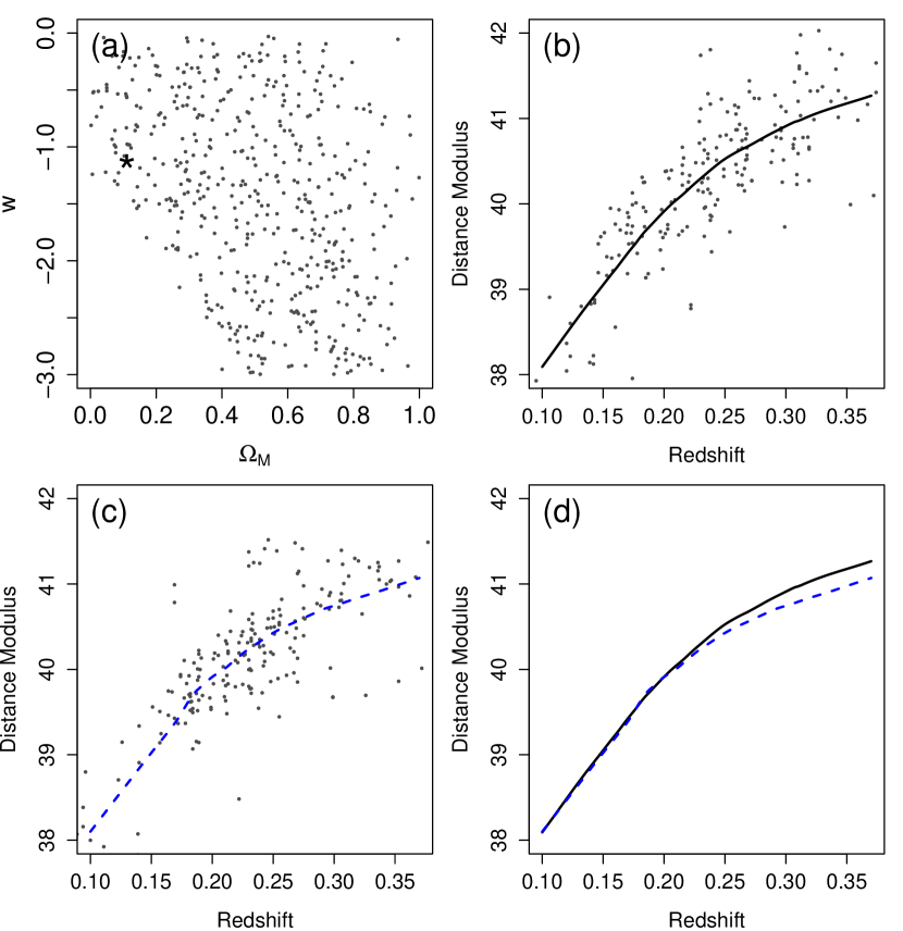
Figure 5: Illustration of key steps of the SMC ABC algorithm in the example. Panel (a): a collection of 500 particles plotted in the relevant parameter space from an intermediate iteration of the SMC ABC algorithm. A random particle is selected, plotted as the star, and perturbed a small amount. Panel (b): the simulated dataset corresponding to the perturbed particle from panel a. The line is a nonparametric smooth of the data and represents the summary statistic. Panel (c): “Observed” data. The dashed line represents a nonparametric smooth of the observed data. Panel (d): a comparison between the simulated and observed datasets via the sum of squared deviations across the length of the curve. The particle is accepted in this iteration even though the curves are discrepant at high redshift as the tolerance is not small enough to reject it. Such a point would likely be rejected in a future iteration as the tolerance is decreased (see Fig. 6).

Fig. 5 depicts key steps in the SMC algorithm as applied to this situation. The prior is chosen to be uniform over the region $0<\Omega_{M}<1$ and $-3<w<0$. A collection of 500 $(\Omega_{M},w)$ pairs, often called particles in the context of SMC methods, is migrated through the iterations of the algorithm. Fig. 5a shows the collection of 500 particles at the conclusion of one of the early time steps. One of these particles is chosen at random and perturbed a small amount; the parameter combination is $\Omega_{M}=0.11$ and $w=-1.21$, and is shown as the star in the plot. This parameter combination in denoted $\theta_{i}^{t}$ in the algorithm above. Simulated data are created by drawing a collection of 200 $(z,z^{\prime})$ pairs, sampling with replacement, from the collection shown in Fig. 1. With $\theta_{i}^{t}$ specified and the 200 true redshifts, it is trivial to calculate the distance modulus of each SN Ia, and then add uncertainty using a Gaussian PDF with variance $\left(\sigma_{\mu,i}\right)^{2}=0.04$. Fig. 5b shows the resulting simulated distance moduli plotted against the photometric redshifts $z$. The point is that this is a plot that can be created using observable data: these data comprise the ${\bf x}_{i}^{t}$ that appear in the algorithm above.

A key step in any implementation of SMC ABC is the choice of the summary statistic. Here, the summary statistic ${s}_{i}^{t}$ is found by applying a nonparametric regression smoother through these data; this curve is shown in Fig. 5b. (The approach used to perform this smooth is briefly presented in the Appendix.) The motivation for this choice is as follows: as stated above, ideally we would choose a sufficient statistic as our summary statistic. A sufficient statistic is a summary that separates out from the full data that portion which is useful for estimating $\theta$. In this case, we know that the relationship between redshift and distance modulus for fixed $\theta$ is a smooth curve. The deviation of the data from a smooth curve can be solely attributed to random error in the measurements, error which is not all informative of the value of $\theta$. For this reason, it is reasonable to believe that a smoothed version of the points shown in Fig. 5b captures all of the useful information for estimating $\theta$.

The comparison between the real and simulated data will be done via these smooth curves. Fig. 5c shows the observed data, along with the result ${s}$ of applying the same smoothing procedure to these data. Finally, in Fig. 5d, these two curves are compared via a simple distance calculation between these curves, namely, the sum of squared deviations across the length of the curve. The particle is accepted in this iteration, because even though the curves differ at high redshift, the tolerance is not sufficiently small yet to reject at this difference. Fig. 6 shows how the collection 500 particles evolves over the steps of the algorithm. As the steps progress, the particles converge in and approximate a sample from the posterior. The notable feature of this result is that this posterior is centered on the solid contours. Just as in Fig. 4, these contours represent the posterior as derived by someone who had full knowledge of the redshifts. It is clear that by avoiding the unjustified Gaussian assumptions made in § 2, the bias that was present in the previous posterior based on photometric redshifts has been removed.

4 SMC ABC Cosmology with SDSS-II Supernovae

In this section we apply SMC ABC to first year data from the SDSS-II Supernova Survey (Holtzman et al., 2008; Kessler et al., 2009a). The development of the sophisticated supernova simulation and analysis software SNANA (Kessler et al., 2009b) has made possible the comparison between the SDSS-II supernova sample and simulated data sets and is a natural first choice to test ABC methods in cosmology. The purpose of this section is to demonstrate that ABC can be used to estimate an accurate posterior distribution. We use the spectroscopically confirmed sample to estimate cosmological parameters from assuming a spatially flat universe and a constant dark energy equation of state parameter, $w$. In this section we discuss how we create simulated data sets, our ABC setup, and compare our posterior distributions for the matter density $\Omega_{M}$ and the equation of state parameter $w$ with those from a $\chi^{2}$ analysis using statistical errors only. We close this section demonstrating the full utility of ABC by including Type IIP supernovae contamination to the SDSS sample and estimating the correct posterior distribution with ABC.

4.1 Simulation Setup

For this analysis we will use data from the fall 2005 SDSS-II Supernova Survey which were published in Holtzman et al. (2008). For detailed information regarding the scientific goals and data processing for the survey we refer the reader to Frieman et al. (2008), to Sako et al. (2008) for details of the supernova search algorithms and spectroscopic observations and to Section 2 of Kessler et al. (2009a) for a brief summary of the survey.

Our goal is to compare the derived posterior distributions for $\Omega_{M}$ and $w$ using ABC with those from Kessler et al. (2009a) which were done using a more traditional $\chi^{2}$ analysis. To make this comparison as meaningful as possible we apply the same relevant selection cuts to the data. Therefore, defining $t_{0}$ as the time of peak brightness in rest-frame B according to MLCS2k2 such that $t-t_{0}=0$, we require for each SN Ia light curve, one measurement before peak brightness and one measurement more than 10 days after peak brightness. Additionally we require five measurements with $-15<t-t_{0}<60$ days. These requirements ensure adequate time sampling to yield a robust light-curve model fit. Kessler et al. (2009a) additionally require one measurement in $gri$ with a signal-to-noise greater than 5 to put a floor on the quality of data and require $P_{\rm fit}>0.001$, where $P_{\rm fit}$ is MLCS2k2 light-curve fit probability based on $\chi^{2}$. This requirement is designed to remove obvious peculiar SNe Ia in an objective fashion.

All supernovae in this sample have unambiguous spectroscopic confirmation and we use photometry in $g$, $r$, and $i$ bands. This leaves us with 103 SDSS SNe Ia. This sample is identical to Kessler et al. (2009a)’s sample A and can be taken from their Table 10.

We can broadly separate the treatment of variables in the likelihood into two categories: (1) those which are of cosmological interest and (2) nuisance parameters. One will be able to construct posterior distributions for all parameters in the first category, in this case $\theta=[\Omega_{M},w]$, while sampling from the probability space spanned by the set of nuisance parameters when generating simulated data sets.

We use SNANA to simulate sets of supernovae from different cosmologies. The idea is to randomly sample from the probability distributions of each nuisance parameter every time a simulated set of supernovae is generated. If we were to fix the cosmology and simulate many data sets, the probability space spanned by the nuisance parameters should be reflected in the variance of the sets of simulated data.

Within SNANA we will use the MLCS2k2 model (Jha et al., 2007) to simulate SN Ia light curves. We use the same modified version of MLCS2k2 that was developed and trained in Kessler et al. (2009a). In this model the observed model magnitudes corrected for Galactic extinction, $K$-correction, and time dilation, for each passband, $X$, are given by

$${\bf m}_{X}(t-t_{0}) = {\bf M}^{0}_{X}+\mu_{0}+{\bf\xi}_{X}\left(\alpha_{X}+\frac{\beta_{X}}{R_{V}}\right)A_{V}^{0}$$ (16)

$$+{\bf P}_{X}\Delta+{\bf Q}_{X}\Delta^{2}$$

where ${\bf M}_{X}^{0}$ are the fiducial absolute magnitudes, $\mu_{0}$ is the distance modulus, $R_{V}$ and $A_{V}^{0}$ are the host galaxy extinction parameters, and ${\bf P}_{X}$ and ${\bf Q}_{X}$ describe the change in light-curve shape as a quadratic function of $\Delta$. Quantities that are functions of phase are in bold. ${\bf M}_{X}^{0}$, ${\bf P}_{X}$, and ${\bf Q}_{X}$ are estimated from a training set leaving $t_{0}$, $\mu_{0}$, $\Delta$, $A_{V}^{0}$, and $R_{V}$ as the free parameters.

The distance modulus can be related to the luminosity distance for a flat universe with a constant dark energy equation of state parameter of $w=-1$ in the following way

$$\mu_{0} = 5\log\left(d_{L}/10{\rm pc}\right)$$ (18)

$$= 5\log\left(c(1+z)\int_{0}^{z}\left[\Omega_{M}(1+z^{\prime})^{3}+\Omega_{\Lambda}\right]^{1/2}dz^{\prime}\right)$$

$$-5\log{H_{0}+25.}$$

Note that a change in $H_{0}$ simply scales the distance modulus. It is easy to see that if one rewrites Eq. 16 in terms of luminosity distance that a degeneracy arises between $H_{0}$ and $M_{V}$. Even if $H_{0}$ is known from some other experiment, $M_{V}$ would still need to be marginalized over.

$\xi_{X}$ is defined as

$$\xi_{X}=\frac{A_{X}}{A_{X}^{0}}$$ (19)

and is equal to unity at maximum light. This framework allows one to separate out the time dependence of the extinction while being insensitive to the total extinction $E(B-V)$ and the extinction law $R_{V}$.

A major advantage of MLCS2k2 is that it allows one to separate reddening resulting from dust in the host galaxy (third term in Eq. 16) from intrinsic color variations of the supernova which are captured by $\Delta$. The validity of this approach depends on how separable these two terms are, how well intrinsic color is predicted by light curve shape, and relies on accurate models of the distribution of extinction with redshift (Wood-Vasey et al., 2007).

To generate a simulated set of data, we assume a flat universe and choose $\Omega_{M}$ and $w$ from flat priors over the range $[0,1]$ and $[-3,0]$ respectively. One could instead draw cosmological parameters from priors based on the SDSS detection of the baryon acoustic oscillations (Eisenstein et al., 2005) and the five-year Wilkinson Microwave Anisotropy Probe observations (WMAP-5) of the cosmic microwave background (Komatsu et al., 2009). A random supernova redshift is selected from a power law distribution given by $\frac{dn}{dz}\sim(1+z)^{\beta}$ where $\beta=1.5\pm 0.6$ (Dilday et al., 2008). $\Delta$ and $A_{V}$ are then drawn from empirical distributions determined in Section 7.3 of Kessler et al. (2009a). Using the parameterization of Cardelli et al. (1989) to describe the extinction with $R_{V}=2.18$ (as determined from Section 7.2 in Kessler et al. 2009a), the MLCS2k2 light-curve model can now be used to generate supernovae magnitudes which are then $K$-corrected using spectral templates from Hsiao et al. (2007) into observer frame magnitudes.

SNANA then chooses a random sky coordinate consistent with the observed survey area and applies Galactic extinction using the Schlegel et al. (1998) dust maps, chooses a random date for peak brightness, and selects observed epochs from actual SDSS survey observations. Noise is simulated for each epoch and filter and includes Poisson fluctuations from the SN Ia flux, sky background, CCD read noise, and host galaxy background.

The simulation allows one to add additional intrinsic variations in SN Ia properties to better match the observed scatter in the Hubble diagram. We do this by “color smearing.” A magnitude fluctuation drawn from a Gaussian distribution is added to the rest-frame magnitude for each passband leading to a change in model colors of $\sim 0.1$ mag. SNANA also includes options to model the search efficiency of the survey.

The aforementioned selection cuts on the observed data are then applied to the simulated data. This process is done for a selected cosmology for $\sim 100$ SN Ia over the redshift range of $[0.02,0.45]$, similar to the SDSS data, assuming a redshift uncertainty of 0.0005. Finally, the distance modulus is measured by performing an MLCS2k2 light curve fit assuming the same prior on $A_{V}$ and $\Delta$ from which the data were simulated.

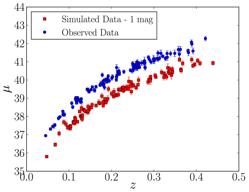
Figure 7: Hubble diagram for the observed data in blue and a simulated dataset in red. The simulated dataset is offset from the observed data by 1 mag and was generated assuming $\Omega_{M}=0.3$ and $w=-1.0$. The distance modulus uncertainties, intrinsic scatter, and redshift distributions are well reproduced in the simulated dataset. Simulated datasets like this one with different cosmologies are used in our ABC analysis.

In Fig. 7 we plot the distance modulus as a function of redshift for the SDSS data in blue and a simulated data set in red. For the simulated data set we assume that $\Omega_{M}=0.3$ and $w=-1.0$. The simulated data have been offset by 1 mag for clarity. The distance modulus uncertainties, intrinsic scatter, and redshift distributions are similar between the simulated and observed data sets.

4.2 SMC ABC Implementation

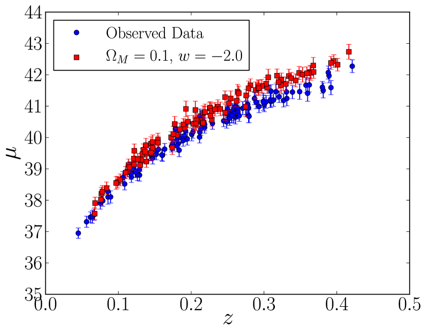
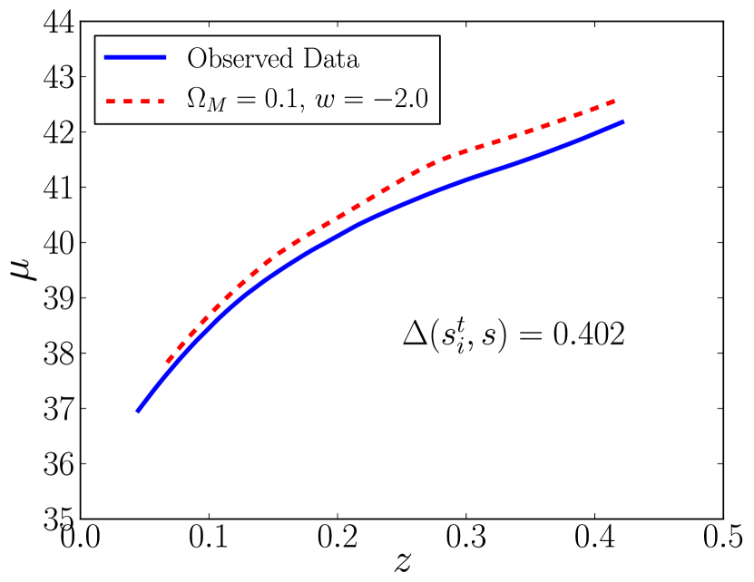
Figure 8: Illustration of the distance metric using SDSS data and simulated data from SNANA. Top: Hubble diagram for the observed data in blue and a simulated dataset in red. The simulated data were generated assuming $\Omega_{M}=0.1$ and $w=-2.0$. Bottom: Nonparametric smooth of the two datasets. The distance metric is defined to be the median absolute deviation between the smoothed curves which is equal to 0.402 for this case. Our final tolerance is 0.033.

To calculate the measure of similarity between the observed and simulated data sets, $\Delta({s}^{t}_{i},{s})$, we turn to the Hubble diagram. In the top panel of Fig. 8 we show $\mu$ versus $z$ for our observed data and a simulated data set with $\Omega_{M}=0.1$, and $w=-2.0$. A reasonable distance measure could be the Euclidean distance between the data sets at the redshifts of the observed data. However, in keeping with the notion of summary statistics, we would like to compare a smooth representation of the two data sets rather than the data themselves. In the bottom panel of Fig. 8 we show a non-parametric smooth of the simulated and observed data. The details on how we perform the non-parametric smooth are in Appendix A. We opt for a non-parametric smooth in the interests of efficiency and to prevent inserting additional assumptions about the data in an intermediate step in contrast to fitting the data with a cosmology fitter. We now define $\Delta({s}^{t}_{i},{s})$ to be the median absolute deviation between the smoothed data sets evaluated at the observed redshifts. We choose this because it is simple, it is robust to poor smoothing at high and low redshifts, and allows for a physical interpretation of the minimum tolerance. Since we are basically measuring the distance between the two data sets in distance modulus, we consider our minimum tolerance to be equal to the median uncertainty in the smoothed observed data, i.e., we declare the observed data and simulated data sets sufficiently similar when the simulated data are within the error of the observed data.

For simplicity in this analysis we fix the value of $H_{0}$ to 65 km s^-1 Mpc^-1 to restrict the relevant region of parameter space. This improves the efficiency of the ABC algorithm and more importantly, makes the comparison between ABC and $\chi^{2}$ more striking. However, we note that for this particular definition of the distance metric the simulated value of $H_{0}$ directly scales $\Delta({s}^{t}_{i},{s})$ in a trivial manner. One could naively treat $H_{0}$ as a nuisance parameter and randomly sample $H_{0}$ from a flat prior over some range. Since $H_{0}$, $w$, and $\Omega_{M}$ are correlated, a faster approach would be to add $H_{0}$ as another cosmological parameter, adding a third dimension to the parameter space. The particles would then trace out the three-dimensional posterior distribution from which one could marginalize over $H_{0}$ to obtain the two-dimensional projection. Given the simulation expense, one would like to take advantage of the simple relationship between $H_{0}$ and $\Delta({s}^{t}_{i},{s})$. To this end one could calculate a set of $\Delta({s}^{t}_{i},{s})$s corresponding to a range of Hubble parameter values for a given $w$ and $\Omega_{M}$. The particle is then accepted with a percentage based on the number of $\Delta({s}^{t}_{i},{s})$ elements that meet the tolerance criterion. This avoids re-simulating data sets a given number of times over a range of $H_{0}$ values while still sampling the probability space fully and thus marginalizing over $H_{0}$.

We choose $\epsilon_{t}$ according to the distribution of $\{\Delta({s}^{t-1}_{i},{s}):i=1,...,N\}$ instead of having a predefined sequence of tolerances to walk though. For the first iteration, we accept all points, i.e., the tolerance is infinite. For the next iteration, $t=2$, the tolerance $\epsilon_{t=2}$ is set to the 25% percentile of $\{\Delta({s}^{1}_{i},{s})\}$. All subsequent $\epsilon$s are the 50% percentile of the previous iteration. A percentile which is too large allows for many acceptances and will not localize into the correct region until $T$ is large. Conversely, if one is too strict in their sequence of tolerances, many simulations are required before a point is accepted. We found that putting a stricter cut on what $\epsilon$ should be early on helps concentrate quickly into the correct area of parameter space, requiring fewer simulations in future iterations.

We define $\epsilon$ to be sufficiently small when it is less than the uncertainty on the non-parametric smooth of the observed data, which we estimate via bootstrap. The median uncertainty on the non-parametric smooth for the SDSS data set is 0.033. We require $\Delta({s}^{t}_{i},{s})$ for each particle to be less than this value at the final iteration.

We choose $N=150$ particles and run the code on eight different processors. As the initial particles are independently drawn between the three runs, the results can be combined to better estimate the posterior distribution. However, the sequence in $\epsilon$ is slightly different for each run. In practice one should parallelize the code at the level of accepting $N$ points so that there is just one sequence of tolerances. Ours do not vary significantly and is not a concern for our demonstration.

Properties of the posterior distribution are then drawn from the final sample of particles and their weights which meet the minimum tolerance criteria.

4.3 Results and Discussion

It is useful to first review the cosmological analysis performed in Kessler et al. (2009a). MLCS2k2 provides an estimate of the distance modulus for each supernova. The $\chi^{2}$ statistic is then calculated over a grid of model parameters and used to derive cosmological parameter estimates. Recall that $-2\ln(\pi(\theta\hskip 0.72229pt|\>{\bf x}))=\chi^{2}$. The $\chi^{2}$ statistic for the SDSS supernova sample is calculated according to

$$\chi^{2}=\sum_{i}\frac{\left[\mu_{i}-\mu_{\rm mod}(z_{i}\hskip 0.72229pt|\>w,\Omega_{M},H_{0})\right]^{2}}{\sigma_{\mu}^{2}}$$ (20)

where $\mu_{i}$ and $z_{i}$ are the distance modulus returned from MLCS2k2 and measured redshift of the supernova, and $\mu_{\rm mod}$ is the model magnitude. The distance modulus uncertainties are given by

$$\sigma_{\mu}^{2}=\left(\sigma_{\mu}^{\rm fit}\right)^{2}+\left(\sigma_{\mu}^{\rm int}\right)^{2}+\left(\sigma_{\mu}^{z}\right)^{2}$$ (21)

where $\sigma_{\mu}^{\rm fit}$ is the statistical uncertainty reported by MLCS2k2, $\sigma_{\mu}^{\rm int}=0.16$ is additional intrinsic error, and

$$\sigma_{\mu}^{z}=\sigma_{z}\left(\frac{5}{\ln{10}}\right)\frac{1+z}{z(1+z/2)}.$$ (22)

The posterior distributions for $\Omega_{M}$ and $w$ assuming a flat universe can then be found by marginalizing over $H_{0}$. Recall for our comparison that we are fixing the value of $H_{0}$ and do not need to marginalize over $H_{0}$.

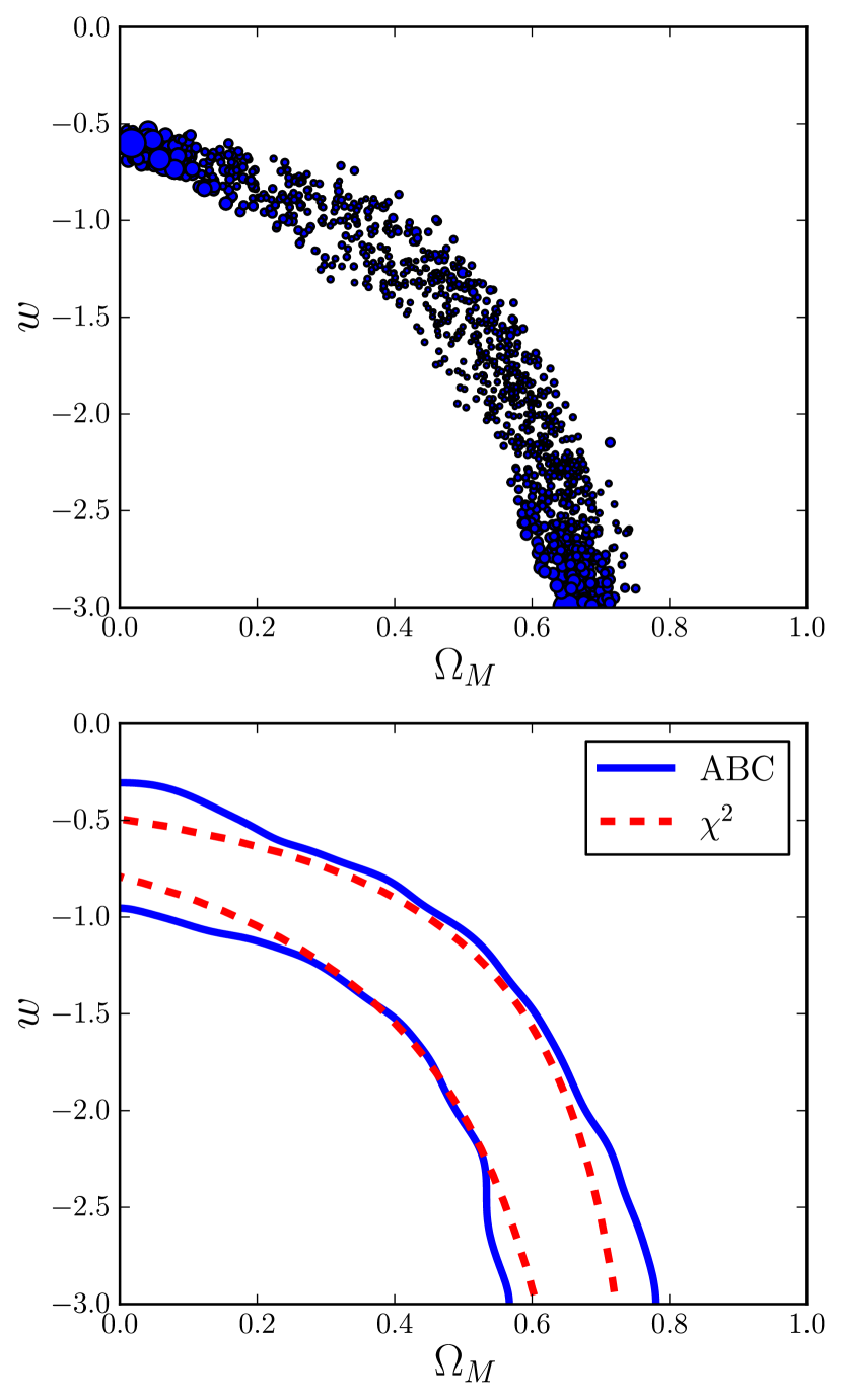
Figure 9: Comparison of SMC ABC with a $\chi^{2}$ analysis. Top: Particles from the final ABC iteration. Bottom: The 95% credible regions from ABC (blue-solid) and $\chi^{2}$ (red-dashed). The contours between ABC and $\chi^{2}$ are well matched except near the boundaries. The discrepancy results from the sharp boundaries of our prior. ABC is attempting to account for the fact that there is relevant parameter space which it cannot explore.

In Fig. 9 we compare our posterior distribution to that found using the approach described above. The top plot shows the particles from the final iteration of the SMC ABC algorithm. The area of the particle symbol represents the weight. These points and their weights represent a sample from the posterior distribution. We estimate the 95% credible region from this sample and compare with the 95% confidence region from a $\chi^{2}$ analysis in the bottom plot. Overall the contours are well matched. The weights on the particles become large just inside the hard boundaries set by the priors on $\Omega_{M}$ and $w$. The algorithm is accounting for the fact that there is parameter space beyond the boundary which it cannot explore. This is similar to an MCMC algorithm running into a boundary and sampling more in that region because it cannot cross the boundary. As a result the ABC contours become wider than those from $\chi^{2}$ near the boundaries.

We reiterate that the goal of this exercise was not to derive new cosmological constraints but merely to see how well we can recover the likelihood contours presented in Kessler et al. (2009a) using a simple implementation of SMC ABC. We demonstrate that we can recover the posterior distribution derived from current analysis techniques with the hope of convincing the reader this approach will be useful in the near future. We do note that the A in ABC stands for “Approximate.” One should expect slight differences in the estimated posterior distributions due to choices of distance metric, summary statistics, and final tolerance.

4.4 Type IIP Contamination

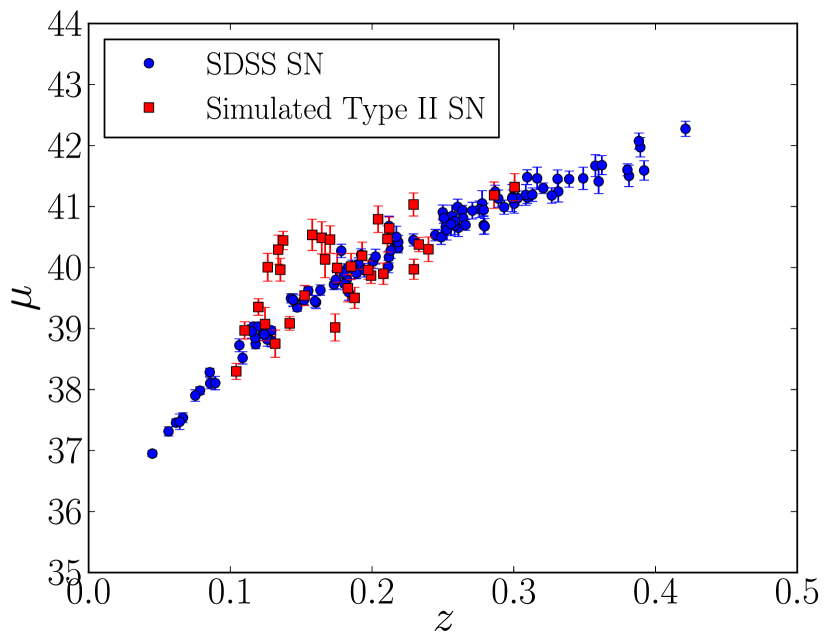
Figure 10: SDSS sample plus 34 Type IIP supernovae simulated with SNANA. This combined dataset is our “observed” sample for the type contamination analysis.

We add 34 simulated Type IIP supernovae to the SDSS sample so that the overall type contamination is 25%. While the amount and type are a bit extreme it is useful for illustrative purposes. We use SNANA to simulate the data which uses spectral templates and smoothed light curves of well observed supernovae. We use the “NONIa” option which computes the observer magnitudes from the spectral energy distribution and we set MAGOFF=-0.6 and MAGSMEAR=0.9. For details on these keywords and additional information on simulating non-Ia light curves we refer the reader to Section 3.5 of the SNANA manual. The selection cuts, other observing parameters, and fitting procedure remain as described in Section 4.1. Our new sample is plotted in Figure 10.

We modify our SMC ABC analysis as follows; after drawing cosmology parameters from $\pi(\theta)$, we simulate and fit additional Type IIP light curves in the aforementioned manner and add those to our simulated Type I data. From this point the SMC ABC algorithm proceeds as before. Our new final tolerance has increased to 0.038 due to the additional scatter in the Hubble diagram.

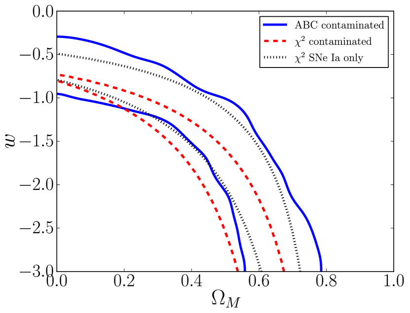
Figure 11: 95% credible region from ABC (blue-solid) and the 95% confidence interval from $\chi^{2}$ for the SDSS sample with type contamination (red-dashed) and the original SDSS sample (black-dotted). The type contamination biases the $\chi^{2}$ result. ABC reproduces the entire credible region without this bias and reflects additional uncertainty due to increased scatter in the Hubble diagram.

The resulting 95% credible region is plotted in Fig. 11 as the blue-solid line along with the 95% confidence regions from $\chi^{2}$ with (red-dashed) and without (black-dotted) type contamination. The contours from the $\chi^{2}$ analysis have shifted due to the type contamination. One can attempt to fix this bias with simulations about the best fit value but one can use SMC ABC to reproduce the full bias-correct contours. The ABC contours are 42% larger in area than the $\chi^{2}$ uncontaminated contours, but cover essentially the same area as the original ABC contours from the uncontaminated sample. If contamination is properly modeled the ABC method is robust against these effects that can only be applied on a population basis rather than as a per-object correction.

It is worthwhile to note that while the division between statistical and systematic errors is often loosely used to make a distinction between uncertainties that will decrease with more data of the same form versus uncertainties that will not decrease with larger sample sizes, the benefit of a forward-modeling framework is that they can be treated consistently and simultaneously. To create a simulation model one is forced to make choices regarding the distributions of all statistical and systematic uncertainties through either analytic or empirical methods. Systematic errors come in at least three flavors: (1) effects that we know and understand and have a reasonable understanding of the relevant input distribution; (2) effects we qualitatively understand, but for which we do not have a good input prior distribution: e.g., $R_{V}$ values in host galaxies. We can compute the effect on a supernova lightcurve, but we are relatively uncertain about the correct distribution of $R_{V}$ in galaxies in the Universe; (3) effects that we lose sleep over but that we have so little understanding of that we cannot model their effects at all, although we may have some purely empirical guidance: spectroscopic selection biases; evolving metallicity content of stars over the last 8 billion years. Systematic errors of type 1 are easy to include in ABC. One can use ABC to examine the effects on the posterior distribution from different choices of distributions for systematic errors of type 2. One may be able to include empirical distributions for systematic errors of type 3. Otherwise ABC can not tell you something about these systematic errors unless they are treated as model parameters. Forward modeling with an SMC ABC approach provides a powerful way to fully incorporate all available knowledge and ignorance.

5 Future Work

We presented here a proof of concept for an SMC ABC method to infer model parameters based on SN Ia measurements. To fully deploy this method will require an incorporation of all data sets and modeling relative systematics between the surveys, e.g., relative calibration. This is tractable, if somewhat tedious, and has been done with varying degrees of completeness already in the literature. Extending this approach to explorations of time-variable dark energy is a simple matter of implementing at different generating model for luminosity distance as a function of redshift.

For future photometric-focused surveys, we would explore more fully the non-Gaussianity of photometric redshifts as derived from calibration samples. The probability distributions for these photometric redshifts will be strongly affected by evolution of the contamination fraction of non-SN Ia with redshift. Once that is phrased as part of the generating model, ABC will incorporate such uncertainties on the same basis as all of the other cosmological and astrophysical parameters.

The ABC+SNANA framework is a very suitable vehicle for testing the effects of different lightcurve fitters on the derived cosmological parameters. ABC will help efficiently determine what different parameter choices in the fitters should be explored.

But the real long-term goal would be to apply the summary statistic comparison at the individual lightcurve level. This could significantly reduce the computing time. The analysis presented in this work with $\sim$100 supernovae and 1200 particles required $\sim$600 CPU-hours. We estimate that a realistic problem with a sample of $10^{4}$ supernovae could be done on $O(10)$ CPU-years, which is within reasonable computing resources. Applying the summary statistic comparison at the individual light curve level rather than in Hubble diagram space bypasses fitting the simulated light curves which currently requires most ($\sim$90%) of the computing time.

Comparing the simulated and observed data at the individual lightcurve level would also be the cleanest framework to explore agreement and evolution of systematics. The only “training” would be in the generation of the templates that the SN Ia are derived from in the first place. The cosmological distance and supernova property comparison would be finally integrated in one direct comparison.

6 Conclusions

We have introduced and demonstrated the use of Approximate Bayesian Computation techniques to address the requirements for analyzing near-future SN Ia cosmological data sets. ABC presents a consistent and efficient approach to explore multi-dimensional non-Gaussian parameter distributions with full incorporation of systematic uncertainties.

• Forward modeling is often the only way to correctly incorporate the full range of statistical and systematic uncertainties in some of the big astronomy questions being addressed today.

• Calculation of likelihood functions for evaluation in a traditional Markov Chain Monte Carlo approach may not be analytically tractable.

• ABC allows for a simultaneous exploration of parameter space and tolerance to create credible regions for physical parameters of interest without the need to construct an explicit likelihood function.

• Sequential Monte Carlo ABC offers an efficient way to explore the full parameter space of all important input parameters and model effects.

• The use of a summary statistic focuses attention directly on the ability to discriminate model parameter values in the relevant space of observed values.

We encourage scientists facing similar problems to consider the use of ABC techniques to increase their incisive power to explore the complicated parameter spaces that are surrounding the key questions in astrophysics and cosmology today.

7 Acknowledgements

We thank the referee for helpful comments and A.W. and M.W.-V. thank Saurabh Jha for insightful discussions. This research was supported in part by NSF DMS-1106956. A.W. and M.W.-V. were supported in part by NSF AST-1028162. A.W. additionally acknowledges support from PITT PACC and the Zaccheus Daniel Foundation.

Appendix A Non-Parametrically Smoothing the Simulated and Observed Data

To perform a non-parametric smooth we use a robust locally weighted regression (loess)(Cleveland, 1979). This routine smooths the data by iteratively fitting a local d-order polynomial to the data using a tricube weighting function. We use a quadratic polynomial and, for the observed data, add an additional weight according to the uncertainty in $\mu$ given by Eq. 21.

We choose the size of the window to locally smooth over by minimizing the risk or the sum of the variance and bias squared. We estimate the risk using the leave-one-out cross validation score

$$R(h)=\frac{1}{N}\sum_{i=0}^{I}(f(x_{i})-f_{(-x_{i})}(x_{i}))^{2}$$ (A1)

where $f(x)$ is the smoothed function using a smoothing window given by $h$ and $f_{(-x_{i})}$ is the smooth obtained leaving out the $i^{\rm th}$ data point (see, e.g., Wasserman (2006)). The smoothing window goes from zero to one with zero being no smooth and one resulting in a line. Using the SDSS data we find the minimum risk to yield a smoothing window of 0.52. As estimating the risk is somewhat computationally intensive, we determine the smoothing window using the observed data and use the same window to smooth the simulated data in the ABC algorithm.

Figure 2: Comparison between the assumed Gaussian joint distribution between $z$ and $\zeta_{i}$ (dashed) and nonparametric fits (solid) through the simulated data shown in Fig. 1. Three cross-sections are shown, one at each of photometric redshifts of $0.1$, $0.2$, and $0.3$. In each case, a bin of width 0.02 is constructed, centered on these values, and the observations which fall into this bin are used to estimate the distribution for spectroscopic redshift. A Gaussian is not a terrible approximation to these cross-sections, but is it far from ideal.

Figure 3: Distance modulus residual defined as $\mu(\zeta_{i},\theta)-\mu(z_{i},\theta)$ as a function of photometric redshift $z_{i}$. Under the described Gaussian approximation, these distributions should all have mean zero. The boxplots compare the distribution in different narrow redshift bins. The top and bottom of the box indicate the 25th and 75th percentile, the center line marks the median, and the “whiskers” mark 1.5 times the inter-quartile range. Points outside the whiskers are considered outliers. The “notch” in each boxplot allows for comparison to determine statistical significance: if the notches of two boxes do not overlap, then there is a statistically significant difference between the medians of the populations. Hence, it is evident that there is a bias introduced; the centers of these distributions are not always zero. This bias indicates that the Gaussian model for the joint distribution of ($\zeta,z$) is inappropriate.

Figure 6: Progress of the ABC SMC algorithm in estimating the posterior distribution for the toy example. As $\epsilon$ decreases, the collection of particles converges to a sample from the posterior (when the weights are taken into account). The solid contour is the 95% credible region that would have been formed by someone who had knowledge of the spectroscopic redshifts. The dashed contours result from fitting to the output of the ABC algorithm. Compare with Fig. 4 to note the reduction of the bias that resulted from the Gaussian approximation. Note that it is not expected that these contours will be the same, as the ABC simulations are built upon data using photometric redshifts; hence, there is additional uncertainty in the parameter estimates.

References

- Amanullah et al. (2010) Amanullah, R., Lidman, C., Rubin, D., Aldering, G., Astier, P., Barbary, K., Burns, M. S., Conley, A., Dawson, K. S., Deustua, S. E., Doi, M., Fabbro, S., Faccioli, L., Fakhouri, H. K., Folatelli, G., Fruchter, A. S., Furusawa, H., Garavini, G., Goldhaber, G., Goobar, A., Groom, D. E., Hook, I., Howell, D. A., Kashikawa, N., Kim, A. G., Knop, R. A., Kowalski, M., Linder, E., Meyers, J., Morokuma, T., Nobili, S., Nordin, J., Nugent, P. E., Östman, L., Pain, R., Panagia, N., Perlmutter, S., Raux, J., Ruiz-Lapuente, P., Spadafora, A. L., Strovink, M., Suzuki, N., Wang, L., Wood-Vasey, W. M., Yasuda, N., & Supernova Cosmology Project, T. 2010, ApJ, 716, 712
- Astier et al. (2006) Astier, P., Guy, J., Regnault, N., Pain, R., Aubourg, E., Balam, D., Basa, S., Carlberg, R. G., Fabbro, S., Fouchez, D., Hook, I. M., Howell, D. A., Lafoux, H., Neill, J. D., Palanque-Delabrouille, N., Perrett, K., Pritchet, C. J., Rich, J., Sullivan, M., Taillet, R., Aldering, G., Antilogus, P., Arsenijevic, V., Balland, C., Baumont, S., Bronder, J., Courtois, H., Ellis, R. S., Filiol, M., Gonçalves, A. C., Goobar, A., Guide, D., Hardin, D., Lusset, V., Lidman, C., McMahon, R., Mouchet, M., Mourao, A., Perlmutter, S., Ripoche, P., Tao, C., & Walton, N. 2006, A&A, 447, 31
- Barlow (2003) Barlow, R. 2003, ArXiv Physics e-prints
- Barnes et al. (2011) Barnes, C., Filippi, S., Stumpf, M. P. H., & Thorne, T. 2011, ArXiv e-prints, 1106.6281
- Beaumont et al. (2009) Beaumont, M. A., Cornuet, J.-M., Marin, J.-M., & Robert, C. P. 2009, Biometrika, 96, 983
- Beaumont et al. (2002) Beaumont, M. A., Zhang, W., & Balding, D. J. 2002, Genetics, 162, 2025
- Blum & Francois (2010) Blum, M. G. B. & Francois, O. 2010, Statistics and Computing, 20, 63
- Blum et al. (2012) Blum, M. G. B., Nunes, M. A., Prangle, D., & Sisson, S. A. 2012, ArXiv e-prints, 1202.3819
- Cameron & Pettitt (2012) Cameron, E. & Pettitt, A. N. 2012, ArXiv e-prints, 1202.1426
- Cardelli et al. (1989) Cardelli, J. A., Clayton, G. C., & Mathis, J. S. 1989, ApJ, 345, 245
- Cleveland (1979) Cleveland, W. S. 1979, Journal of the American Statistical Association, 74, 829 linklabel
- Conley et al. (2011) Conley, A., Guy, J., Sullivan, M., Regnault, N., Astier, P., Balland, C., Basa, S., Carlberg, R. G., Fouchez, D., Hardin, D., Hook, I. M., Howell, D. A., Pain, R., Palanque-Delabrouille, N., Perrett, K. M., Pritchet, C. J., Rich, J., Ruhlmann-Kleider, V., Balam, D., Baumont, S., Ellis, R. S., Fabbro, S., Fakhouri, H. K., Fourmanoit, N., González-Gaitán, S., Graham, M. L., Hudson, M. J., Hsiao, E., Kronborg, T., Lidman, C., Mourao, A. M., Neill, J. D., Perlmutter, S., Ripoche, P., Suzuki, N., & Walker, E. S. 2011, ApJS, 192, 1
- Contreras et al. (2010) Contreras, C., Hamuy, M., Phillips, M. M., Folatelli, G., Suntzeff, N. B., Persson, S. E., Stritzinger, M., Boldt, L., González, S., Krzeminski, W., Morrell, N., Roth, M., Salgado, F., José Maureira, M., Burns, C. R., Freedman, W. L., Madore, B. F., Murphy, D., Wyatt, P., Li, W., & Filippenko, A. V. 2010, AJ, 139, 519
- Cowles & Carlin (1996) Cowles, M. K. & Carlin, B. P. 1996, Journal of the American Statistical Association, 91, pp. 883 [LINK]
- Dilday et al. (2008) Dilday, B., Kessler, R., Frieman, J. A., Holtzman, J., Marriner, J., Miknaitis, G., Nichol, R. C., Romani, R., Sako, M., Bassett, B., Becker, A., Cinabro, D., DeJongh, F., Depoy, D. L., Doi, M., Garnavich, P. M., Hogan, C. J., Jha, S., Konishi, K., Lampeitl, H., Marshall, J. L., McGinnis, D., Prieto, J. L., Riess, A. G., Richmond, M. W., Schneider, D. P., Smith, M., Takanashi, N., Tokita, K., van der Heyden, K., Yasuda, N., Zheng, C., Barentine, J., Brewington, H., Choi, C., Crotts, A., Dembicky, J., Harvanek, M., Im, M., Ketzeback, W., Kleinman, S. J., Krzesiński, J., Long, D. C., Malanushenko, E., Malanushenko, V., McMillan, R. J., Nitta, A., Pan, K., Saurage, G., Snedden, S. A., Watters, S., Wheeler, J. C., & York, D. 2008, ApJ, 682, 262
- Eisenstein et al. (2005) Eisenstein, D. J., Zehavi, I., Hogg, D. W., Scoccimarro, R., Blanton, M. R., Nichol, R. C., Scranton, R., Seo, H.-J., Tegmark, M., Zheng, Z., Anderson, S. F., Annis, J., Bahcall, N., Brinkmann, J., Burles, S., Castander, F. J., Connolly, A., Csabai, I., Doi, M., Fukugita, M., Frieman, J. A., Glazebrook, K., Gunn, J. E., Hendry, J. S., Hennessy, G., Ivezić, Z., Kent, S., Knapp, G. R., Lin, H., Loh, Y.-S., Lupton, R. H., Margon, B., McKay, T. A., Meiksin, A., Munn, J. A., Pope, A., Richmond, M. W., Schlegel, D., Schneider, D. P., Shimasaku, K., Stoughton, C., Strauss, M. A., SubbaRao, M., Szalay, A. S., Szapudi, I., Tucker, D. L., Yanny, B., & York, D. G. 2005, ApJ, 633, 560
- Fearnhead & Prangle (2012) Fearnhead, P. & Prangle, D. 2012, Journal Of The Royal Statistical Society Series B, 74
- Filippi et al. (2011) Filippi, S., Barnes, C., & Stumpf, M. P. H. 2011, ArXiv e-prints, 1106.6280
- Frieman et al. (2008) Frieman, J. A., Bassett, B., Becker, A., Choi, C., Cinabro, D., DeJongh, F., Depoy, D. L., Dilday, B., Doi, M., Garnavich, P. M., Hogan, C. J., Holtzman, J., Im, M., Jha, S., Kessler, R., Konishi, K., Lampeitl, H., Marriner, J., Marshall, J. L., McGinnis, D., Miknaitis, G., Nichol, R. C., Prieto, J. L., Riess, A. G., Richmond, M. W., Romani, R., Sako, M., Schneider, D. P., Smith, M., Takanashi, N., Tokita, K., van der Heyden, K., Yasuda, N., Zheng, C., Adelman-McCarthy, J., Annis, J., Assef, R. J., Barentine, J., Bender, R., Blandford, R. D., Boroski, W. N., Bremer, M., Brewington, H., Collins, C. A., Crotts, A., Dembicky, J., Eastman, J., Edge, A., Edmondson, E., Elson, E., Eyler, M. E., Filippenko, A. V., Foley, R. J., Frank, S., Goobar, A., Gueth, T., Gunn, J. E., Harvanek, M., Hopp, U., Ihara, Y., Ivezić, Ž., Kahn, S., Kaplan, J., Kent, S., Ketzeback, W., Kleinman, S. J., Kollatschny, W., Kron, R. G., Krzesiński, J., Lamenti, D., Leloudas, G., Lin, H., Long, D. C., Lucey, J., Lupton, R. H., Malanushenko, E., Malanushenko, V., McMillan, R. J., Mendez, J., Morgan, C. W., Morokuma, T., Nitta, A., Ostman, L., Pan, K., Rockosi, C. M., Romer, A. K., Ruiz-Lapuente, P., Saurage, G., Schlesinger, K., Snedden, S. A., Sollerman, J., Stoughton, C., Stritzinger, M., Subba Rao, M., Tucker, D., Vaisanen, P., Watson, L. C., Watters, S., Wheeler, J. C., Yanny, B., & York, D. 2008, AJ, 135, 338
- Fu & Li (1997) Fu, Y. X. & Li, W. H. 1997, Molecular Biology and Evolution, 14, 195
- Ganeshalingam et al. (2010) Ganeshalingam, M., Li, W., Filippenko, A. V., Anderson, C., Foster, G., Gates, E. L., Griffith, C. V., Grigsby, B. J., Joubert, N., Leja, J., Lowe, T. B., Macomber, B., Pritchard, T., Thrasher, P., & Winslow, D. 2010, ApJS, 190, 418
- Hicken et al. (2012) Hicken, M., Challis, P., Kirshner, R. P., Rest, A., Cramer, C. E., Wood-Vasey, W. M., Bakos, G., Berlind, P., Brown, W. R., Caldwell, N., Calkins, M., Currie, T., de Kleer, K., Esquerdo, G., Everett, M., Falco, E., Fernandez, J., Friedman, A. S., Groner, T., Hartman, J., Holman, M. J., Hutchins, R., Keys, S., Kipping, D., Latham, D., Marion, G. H., Narayan, G., Pahre, M., Pal, A., Peters, W., Perumpilly, G., Ripman, B., Sipocz, B., Szentgyorgyi, A., Tang, S., Torres, M. A. P., Vaz, A., Wolk, S., & Zezas, A. 2012, ApJS, 200, 12
- Hicken et al. (2009) Hicken, M., Wood-Vasey, W. M., Blondin, S., Challis, P., Jha, S., Kelly, P. L., Rest, A., & Kirshner, R. P. 2009, ApJ, 700, 1097
- Holtzman et al. (2008) Holtzman, J. A., Marriner, J., Kessler, R., Sako, M., Dilday, B., Frieman, J. A., Schneider, D. P., Bassett, B., Becker, A., Cinabro, D., DeJongh, F., Depoy, D. L., Doi, M., Garnavich, P. M., Hogan, C. J., Jha, S., Konishi, K., Lampeitl, H., Marshall, J. L., McGinnis, D., Miknaitis, G., Nichol, R. C., Prieto, J. L., Riess, A. G., Richmond, M. W., Romani, R., Smith, M., Takanashi, N., Tokita, K., van der Heyden, K., Yasuda, N., & Zheng, C. 2008, AJ, 136, 2306
- Hsiao et al. (2007) Hsiao, E. Y., Conley, A., Howell, D. A., Sullivan, M., Pritchet, C. J., Carlberg, R. G., Nugent, P. E., & Phillips, M. M. 2007, ApJ, 663, 1187
- Jha et al. (2007) Jha, S., Riess, A. G., & Kirshner, R. P. 2007, ApJ, 659, 122
- Kessler et al. (2009a) Kessler, R., Becker, A. C., Cinabro, D., Vanderplas, J., Frieman, J. A., Marriner, J., Davis, T. M., Dilday, B., Holtzman, J., Jha, S. W., Lampeitl, H., Sako, M., Smith, M., Zheng, C., Nichol, R. C., Bassett, B., Bender, R., Depoy, D. L., Doi, M., Elson, E., Filippenko, A. V., Foley, R. J., Garnavich, P. M., Hopp, U., Ihara, Y., Ketzeback, W., Kollatschny, W., Konishi, K., Marshall, J. L., McMillan, R. J., Miknaitis, G., Morokuma, T., Mörtsell, E., Pan, K., Prieto, J. L., Richmond, M. W., Riess, A. G., Romani, R., Schneider, D. P., Sollerman, J., Takanashi, N., Tokita, K., van der Heyden, K., Wheeler, J. C., Yasuda, N., & York, D. 2009a, ApJS, 185, 32
- Kessler et al. (2009b) Kessler, R., Bernstein, J. P., Cinabro, D., Dilday, B., Frieman, J. A., Jha, S., Kuhlmann, S., Miknaitis, G., Sako, M., Taylor, M., & Vanderplas, J. 2009b, PASP, 121, 1028
- Knop et al. (2003) Knop, R. A., Aldering, G., Amanullah, R., Astier, P., Blanc, G., Burns, M. S., Conley, A., Deustua, S. E., Doi, M., Ellis, R., Fabbro, S., Folatelli, G., Fruchter, A. S., Garavini, G., Garmond, S., Garton, K., Gibbons, R., Goldhaber, G., Goobar, A., Groom, D. E., Hardin, D., Hook, I., Howell, D. A., Kim, A. G., Lee, B. C., Lidman, C., Mendez, J., Nobili, S., Nugent, P. E., Pain, R., Panagia, N., Pennypacker, C. R., Perlmutter, S., Quimby, R., Raux, J., Regnault, N., Ruiz-Lapuente, P., Sainton, G., Schaefer, B., Schahmaneche, K., Smith, E., Spadafora, A. L., Stanishev, V., Sullivan, M., Walton, N. A., Wang, L., Wood-Vasey, W. M., & Yasuda, N. 2003, ApJ, 598, 102
- Komatsu et al. (2009) Komatsu, E., Dunkley, J., Nolta, M. R., Bennett, C. L., Gold, B., Hinshaw, G., Jarosik, N., Larson, D., Limon, M., Page, L., Spergel, D. N., Halpern, M., Hill, R. S., Kogut, A., Meyer, S. S., Tucker, G. S., Weiland, J. L., Wollack, E., & Wright, E. L. 2009, ApJS, 180, 330
- Kowalski et al. (2008) Kowalski, M., Rubin, D., Aldering, G., Agostinho, R. J., Amadon, A., Amanullah, R., Balland, C., Barbary, K., Blanc, G., Challis, P. J., Conley, A., Connolly, N. V., Covarrubias, R., Dawson, K. S., Deustua, S. E., Ellis, R., Fabbro, S., Fadeyev, V., Fan, X., Farris, B., Folatelli, G., Frye, B. L., Garavini, G., Gates, E. L., Germany, L., Goldhaber, G., Goldman, B., Goobar, A., Groom, D. E., Haissinski, J., Hardin, D., Hook, I., Kent, S., Kim, A. G., Knop, R. A., Lidman, C., Linder, E. V., Mendez, J., Meyers, J., Miller, G. J., Moniez, M., Mourão, A. M., Newberg, H., Nobili, S., Nugent, P. E., Pain, R., Perdereau, O., Perlmutter, S., Phillips, M. M., Prasad, V., Quimby, R., Regnault, N., Rich, J., Rubenstein, E. P., Ruiz-Lapuente, P., Santos, F. D., Schaefer, B. E., Schommer, R. A., Smith, R. C., Soderberg, A. M., Spadafora, A. L., Strolger, L.-G., Strovink, M., Suntzeff, N. B., Suzuki, N., Thomas, R. C., Walton, N. A., Wang, L., Wood-Vasey, W. M., & Yun, J. L. 2008, ApJ, 686, 749
- Lampeitl et al. (2010) Lampeitl, H., Nichol, R. C., Seo, H.-J., Giannantonio, T., Shapiro, C., Bassett, B., Percival, W. J., Davis, T. M., Dilday, B., Frieman, J., Garnavich, P., Sako, M., Smith, M., Sollerman, J., Becker, A. C., Cinabro, D., Filippenko, A. V., Foley, R. J., Hogan, C. J., Holtzman, J. A., Jha, S. W., Konishi, K., Marriner, J., Richmond, M. W., Riess, A. G., Schneider, D. P., Stritzinger, M., van der Heyden, K. J., Vanderplas, J. T., Wheeler, J. C., & Zheng, C. 2010, MNRAS, 401, 2331
- Law et al. (2009) Law, N. M., Kulkarni, S. R., Dekany, R. G., Ofek, E. O., Quimby, R. M., Nugent, P. E., Surace, J., Grillmair, C. C., Bloom, J. S., Kasliwal, M. M., Bildsten, L., Brown, T., Cenko, S. B., Ciardi, D., Croner, E., Djorgovski, S. G., van Eyken, J., Filippenko, A. V., Fox, D. B., Gal-Yam, A., Hale, D., Hamam, N., Helou, G., Henning, J., Howell, D. A., Jacobsen, J., Laher, R., Mattingly, S., McKenna, D., Pickles, A., Poznanski, D., Rahmer, G., Rau, A., Rosing, W., Shara, M., Smith, R., Starr, D., Sullivan, M., Velur, V., Walters, R., & Zolkower, J. 2009, PASP, 121, 1395
- LSST Science Collaborations et al. (2009) LSST Science Collaborations, Abell, P. A., Allison, J., Anderson, S. F., Andrew, J. R., Angel, J. R. P., Armus, L., Arnett, D., Asztalos, S. J., Axelrod, T. S., & et al. 2009, ArXiv e-prints, 0912.0201
- Mandel et al. (2011) Mandel, K. S., Narayan, G., & Kirshner, R. P. 2011, ApJ, 731, 120
- Marin et al. (2011) Marin, J.-M., Pudlo, P., Robert, C. P., & Ryder, R. 2011, ArXiv e-prints, 1101.0955
- Marjoram et al. (2003) Marjoram, P., Molitor, J., Plagnol, V., & Tavaré, S. 2003, Proceedings of the National Academy of Science, 1001, 15324
- Miknaitis et al. (2007) Miknaitis, G., Pignata, G., Rest, A., Wood-Vasey, W. M., Blondin, S., Challis, P., Smith, R. C., Stubbs, C. W., Suntzeff, N. B., Foley, R. J., Matheson, T., Tonry, J. L., Aguilera, C., Blackman, J. W., Becker, A. C., Clocchiatti, A., Covarrubias, R., Davis, T. M., Filippenko, A. V., Garg, A., Garnavich, P. M., Hicken, M., Jha, S., Krisciunas, K., Kirshner, R. P., Leibundgut, B., Li, W., Miceli, A., Narayan, G., Prieto, J. L., Riess, A. G., Salvo, M. E., Schmidt, B. P., Sollerman, J., Spyromilio, J., & Zenteno, A. 2007, ApJ, 666, 674
- Moral et al. (2006) Moral, P. D., Doucet, A., & Jasra, A. 2006, Journal Of The Royal Statistical Society Series B, 68, 411 [LINK]
- Perlmutter et al. (1999) Perlmutter, S., Aldering, G., Goldhaber, G., Knop, R. A., Nugent, P., Castro, P. G., Deustua, S., Fabbro, S., Goobar, A., Groom, D. E., Hook, I. M., Kim, A. G., Kim, M. Y., Lee, J. C., Nunes, N. J., Pain, R., Pennypacker, C. R., Quimby, R., Lidman, C., Ellis, R. S., Irwin, M., McMahon, R. G., Ruiz-Lapuente, P., Walton, N., Schaefer, B., Boyle, B. J., Filippenko, A. V., Matheson, T., Fruchter, A. S., Panagia, N., Newberg, H. J. M., Couch, W. J., & The Supernova Cosmology Project. 1999, ApJ, 517, 565
- Pritchard et al. (1999) Pritchard, J. K., Seielstad, M. T., Perez-Lezaun, A., & Feldman, M. W. 1999, Molecular Biology and Evolution, 16, 1791
- Riess et al. (1998) Riess, A. G., Filippenko, A. V., Challis, P., Clocchiatti, A., Diercks, A., Garnavich, P. M., Gilliland, R. L., Hogan, C. J., Jha, S., Kirshner, R. P., Leibundgut, B., Phillips, M. M., Reiss, D., Schmidt, B. P., Schommer, R. A., Smith, R. C., Spyromilio, J., Stubbs, C., Suntzeff, N. B., & Tonry, J. 1998, AJ, 116, 1009
- Riess et al. (2004) Riess, A. G., Strolger, L.-G., Tonry, J., Casertano, S., Ferguson, H. C., Mobasher, B., Challis, P., Filippenko, A. V., Jha, S., Li, W., Chornock, R., Kirshner, R. P., Leibundgut, B., Dickinson, M., Livio, M., Giavalisco, M., Steidel, C. C., Benítez, T., & Tsvetanov, Z. 2004, ApJ, 607, 665
- Sako et al. (2008) Sako, M., Bassett, B., Becker, A., Cinabro, D., DeJongh, F., Depoy, D. L., Dilday, B., Doi, M., Frieman, J. A., Garnavich, P. M., Hogan, C. J., Holtzman, J., Jha, S., Kessler, R., Konishi, K., Lampeitl, H., Marriner, J., Miknaitis, G., Nichol, R. C., Prieto, J. L., Riess, A. G., Richmond, M. W., Romani, R., Schneider, D. P., Smith, M., Subba Rao, M., Takanashi, N., Tokita, K., van der Heyden, K., Yasuda, N., Zheng, C., Barentine, J., Brewington, H., Choi, C., Dembicky, J., Harnavek, M., Ihara, Y., Im, M., Ketzeback, W., Kleinman, S. J., Krzesiński, J., Long, D. C., Malanushenko, E., Malanushenko, V., McMillan, R. J., Morokuma, T., Nitta, A., Pan, K., Saurage, G., & Snedden, S. A. 2008, AJ, 135, 348
- Schlegel et al. (1998) Schlegel, D. J., Finkbeiner, D. P., & Davis, M. 1998, ApJ, 500, 525
- Sisson et al. (2007) Sisson, S. A., Fan, Y., & Tanaka, M. M. 2007, Proceedings of the National Academy of Science, 104, 1760
- Stritzinger et al. (2011) Stritzinger, M. D., Phillips, M. M., Boldt, L. N., Burns, C., Campillay, A., Contreras, C., Gonzalez, S., Folatelli, G., Morrell, N., Krzeminski, W., Roth, M., Salgado, F., DePoy, D. L., Hamuy, M., Freedman, W. L., Madore, B. F., Marshall, J. L., Persson, S. E., Rheault, J.-P., Suntzeff, N. B., Villanueva, S., Li, W., & Filippenko, A. V. 2011, AJ, 142, 156
- Tavare et al. (1997) Tavare, S. A., Balding, D. J., Griffiths, R. C., & Donnelly, P. 1997, Genetics, 145, 505
- Wasserman (2006) Wasserman, L. 2006, All of Nonparametric Statistics (233 Spring Street, New York, NY 10013,USA: Springer Science+Businesse Media, Inc.)
- Weiss & von Haeseler (1998) Weiss, G. & von Haeseler, A. 1998, Genetics, 149, 1539 [LINK]
- Wood-Vasey et al. (2007) Wood-Vasey, W. M., Miknaitis, G., Stubbs, C. W., Jha, S., Riess, A. G., Garnavich, P. M., Kirshner, R. P., Aguilera, C., Becker, A. C., Blackman, J. W., Blondin, S., Challis, P., Clocchiatti, A., Conley, A., Covarrubias, R., Davis, T. M., Filippenko, A. V., Foley, R. J., Garg, A., Hicken, M., Krisciunas, K., Leibundgut, B., Li, W., Matheson, T., Miceli, A., Narayan, G., Pignata, G., Prieto, J. L., Rest, A., Salvo, M. E., Schmidt, B. P., Smith, R. C., Sollerman, J., Spyromilio, J., Tonry, J. L., Suntzeff, N. B., & Zenteno, A. 2007, ApJ, 666, 694